Evidence of a Shift in the Short-Run Price Elasticity of

93

Evidence of a Shift in the Short-Run Price Elasticity of Gasoline Demand

Jonathan E. Hughes*, Christopher R. Knittel** and Daniel Sperling***

Understanding the sensitivity of gasoline demand to changes in prices and income has important implications for policies related to climate change, optimal taxation and national security. The short-run price and income elasticities of gasoline demand in the United States during the 1970s and 1980s have been studied extensively. However, transportation analysts have hypothesized that behavioral and structural factors over the past several decades have changed the responsiveness of U.S. consumers to changes in gasoline prices. We compare the price and income elasticities of gasoline demand in two periods of similarly high prices from 1975 to 1980 and 2001 to 2006. The short-run price elasticities differ considerably: and range from -0.034 to -0.077 during 2001 to 2006, versus -0.21 to -0.34 for 1975 to 1980. The estimated short-run income elasticities range from 0.21 to 0.75 and when estimated with the same models are not significantly different between the two periods.

1. IntRoDuctIon

The short-run price and income elasticities of gasoline demand have been studied extensively in the literature. Dahl and Sterner (1991) and more re-cently, Espey (1998) provide thorough reviews based on hundreds of gasoline demand studies. However, past research has been primarily focused on the 1970s

The Energy Journal, Vol. 29, No. 1. Copyright ©2008 by the IAEE. All rights reserved.

* Institute of Transportation Studies, University of California, Davis, One Shields Avenue, Davis, CA 95616. Email: [email protected].

** Department of Economics, University of California, Davis; University of California Energy Institute; Institute of Transportation; and NBER. Email: [email protected].

*** Institute of Transportation Studies, University of California, Davis, One Shields Avenue, Davis, CA 95616. Email: [email protected].

We thank Severin Borenstein, Arthur Havenner, Oscar Jorda, four anonymous referees and a variety of seminar participants for helpful comments. Hughes and Sperling thank the Hydrogen Pathways program and the UC Davis Institute of Transportation Studies for supporting this research. Knittel thanks the University of California Energy Institute for financial support.

94 / The Energy Journal

and early 1980s. Since that time, a number of structural and behavioral changes have occurred in the U.S. gasoline market. Transportation analysts have hypoth-esized that factors such as changing land-use patterns, the implementation of the Corporate Average Fuel Economy program (CAFE), the growth of multiple in-come households and per capita disposable income, as well as a decrease in the availability of non-auto modes such as transit, have changed the responsiveness of U.S. consumers to changes in gasoline prices. For example, a recent analy-sis of household data suggests that suburban households drive 31 to 35 percent more than their urban counterparts, Kahn (2000). In another study, Polzin and Chu (2005) find that the share of transit passenger miles traveled relative to other modes has steadily decreased over the past thirty years suggesting that U.S. con-sumers may be more dependent on automobiles than in previous decades.

Given recent interest in decreasing U.S. gasoline consumption and trans-portation related greenhouse gas emissions, there is a renewed interest in price-based policies such as gasoline or carbon taxes. In this context, it is especially important to consider whether gasoline demand elasticities have changed. This paper focuses on the short-run price and income elasticities of gasoline demand. Historically, estimates of gasoline demand elasticities have proven to be fairly robust. In their survey, Dahl and Sterner (1991) determine an average short-run price elasticity of gasoline demand of -0.26 and an average short-run income elasticity of gasoline demand of 0.48. Based on over 300 prior estimates for the U.S. and other developed countries, Espey (1998) finds a median short-run price elasticity of -0.23 and a median short-run income elasticity of 0.39. In a study of U.S. gasoline demand, Espey (1996) suggests that the magnitude of the short-run gasoline demand elasticity has in fact decreased in magnitude over time. Unfor-tunately, none of these studies allow for a direct comparison between historical elasticities and elasticities today as the studies surveyed in each of these papers are limited to the gasoline market of several decades past.1

Several authors have investigated U.S. demand for gasoline in more re-cent years. Puller and Greening (1999) and Nicol (2003) study the household demand for gasoline using data from the U.S. Consumer Expenditure Survey. Schmalensee and Stoker (1999) investigate the role of household characteristics on gasoline demand using data from the Residential Transportation Energy Con-sumption Survey. Kayser (2000) conducts a similar study using data from the Panel Study of Income Dynamics and includes adjustments in household vehicle stock. Finally, Small and Van Dender (2007) investigate the rebound effect in the U.S. using annual cross-sectional time-series data at the U.S. state-level from 1966 to 2001. Small and Van Dender model explicitly the simultaneous aggre-gate demand for vehicle miles traveled, vehicle stock and fuel economy. They distinguish between the cost per mile of travel and the cost per gallon of fuel and therefore can estimate the price elasticity of gasoline in addition to exogenous and endogenous changes in fuel efficiency. In their analysis, the short-run elastici-ties of miles driven and fuel consumption with respect to fuel price are found to

1. The most recent study surveyed by Espey (1998) contains data from 1993.

Evidence of a Shift in the Short-Run Price Elasticity of Gasoline Demand / 95

decrease from -0.045 and -0.089 at the 1966-2001 sample average to -0.022 and -0.067 for 1997-2001 average values.

In this paper we estimate the short-run price and income elasticities of gasoline demand using a consistent dataset that spans the 1970s and 2000s. This enables a direct comparison of the price and income elasticities of the 1970s and 1980s with today. We investigate gasoline demand in two periods, from Novem-ber 1975 through November 1980 and from March 2001 through March 2006. The periods are chosen because of the similarities in the real retail price of gaso-line and price increases. Because elasticity estimates vary according to data type and empirical model specification (Espey, 1998), we use a consistent set of data and models between the two periods. The models are similar in form to those used in previous studies of gasoline demand. Average U.S. per capita gasoline consumption and personal disposable income data are used in addition to aver-age U.S. retail prices. Our estimates of the short-run price elasticity of gasoline demand for the period from 1975 to 1980 range between -0.21 and -0.34 and are consistent with previous results from the literature. For the period from 2001 to 2006 our estimates of price elasticity range from -0.034 to -0.077. The estimated short-run income elasticities range from 0.21 to 0.75 and when estimated with the same models are not significantly different between the two periods.

We conclude that the short-run price elasticity of gasoline demand is significantly more inelastic today than in previous decades. In the short-run, con-sumers appear significantly less responsive to gasoline price increases. We specu-late about a number of possible explanations for this result in terms of shifts in land-use, social or vehicle characteristics during the past several decades. Finally, we explore policy implications in light of future efforts to reduce U.S. gasoline consumption.

2. BaSIc MoDEl anD Data

2.1 Basic Model

The econometric models used in this paper reflect previous studies of gasoline demand. 2 Our base model specifies the log of gasoline consumption as a function of the log of price and income. Specifically, we estimate:3

lnGjt = b

o + b

1 lnP

jt + b

2 lnY

jt + e

j + e

jt (1)

where Gjt is per capita gasoline consumption in gallons in month j and year t, P

jt

is the real retail price of gasoline in month j and year t, Yjt is real per capita dis-

posable income in month j and year t, ej represents unobserved demand factors

that vary at the month level and ejt is a mean zero error term. Both Y

jt and P

jt are

2. For example see Dahl (1979) or Houthakker et. al. (1974).3. In the context of cointegration or error-correction modeling, Equation (1) could be interpreted

as a long-run structural relationship.


in constant 2000 dollars. We model the ej’s as fixed month effects to capture the

seasonality present in gasoline consumption. Although some, including Hsing (1990), have rejected the double-log

functional form, it is a common specification used in a large number of previous studies. It is adopted here as it provides a good fit to the data and allows for direct comparison with previous results from the literature. Regardless, we also present results for linear and semi-log specifications.

2.2 Basic Model Data

The data used in the analysis are U.S. aggregate monthly data reported by several U.S. government agencies for the period from January 1974 to March 2006.4 Gasoline consumption is approximated as monthly “product supplied” reported by the U.S. Energy Information Administration (2006), which is cal-culated as domestic production plus imports, less exports and changes to stocks. Real gasoline prices are U.S. city average prices for unleaded regular fuel from the U.S. Bureau of Labor Statistics (2006), CPI-Average Price Data.5 Personal disposable income is from the U.S. Bureau of Economic Analysis (2006), Na-tional Economic Accounts. Prices and income are converted to constant 2000 dollars using GDP implicit price deflators from the Bureau of Economic Analy-sis (2006).

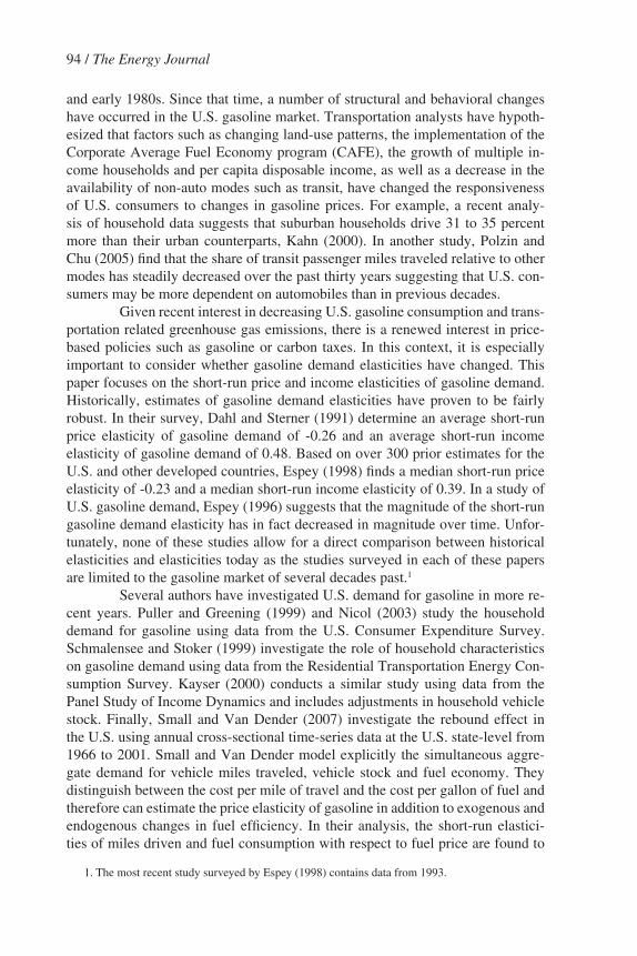
Figure 1 below shows per capita monthly gasoline consumption and real prices for the period from January 1974 to March 2006. In order to compare gaso-line demand elasticities today with those of previous decades, two 5-year periods were selected for analysis, November 1975 through November 1980 and March 2001 through March 2006. Figure 2 below shows the monthly real retail price of gasoline for each period. The peak price in each case is approximately $2.50 per gallon with a slightly higher price in the more recent period. The peak price in both cases represents an increase of approximately $1.00 relative to the price at the beginning of the period. In addition, the average monthly per capita gasoline consumption is roughly equivalent between the two periods with mean 40.4 gal per. month and 39.2 gal. per month and standard deviation of 2.8 gal/month and 1.7 gal/month for the 1975-1980 and 2001-2006 periods, respectively.

The choice of these two periods is an attempt to control for the potential effect of price and on the estimated elasticities. While the two periods exhibit remarkably similar price increases, given the nature of real economic data, some variation is inevitable. The potential impact of these differences on the estimated elasticities is difficult to predict. Because the peak price is higher and the price spikes are sharper in the 2001 to 2006 data, one might expect the price elasticity to be more elastic during this period. Alternatively, the period from 1975 to 1980

4. Aggregate data are used due to the lack of data at the regional or state-level for all independent variables in the appropriate time period.

5. Price data on unleaded regular were unavailable prior to 1976 and as a result, 1975 data are for leaded regular.


Figure 1. Monthly Per capita Gasoline consumption and Real Retail Gasoline Price for January 1974 to March 2006

Figure 2. Real Retail Gasoline Price for two Periods from november 1975 through november 1980 and March 2001 through March 2006


is characterized by a longer period of elevated prices which might tend to increase elasticity by allowing consumers more time to adjust to elevated prices. Price volatility, such as in the period from 2001 to 2006, may also play the opposite role if consumers perceive price fluctuations as temporary. In this case, consum-ers may be less likely to alter their behavior in response to price changes. All in all however, the real price data are remarkably similar between the two periods providing for a suitable comparison of elasticity estimates.

2.3 time Series Properties of the Data

The autocorrelation plots of consumption, prices and income suggest the presence of a unit root in each series; this is corroborated by Elliot-Rothenberg-Stock unit root tests where we fail to reject a unit root for each series.6 Given these results, our demand model can be viewed as a cointegrating regression model. Stock (1987) shows that provided our residuals are stationary, our parameters are super-consistent, implying they converge at a speed of T, rather than root-T.

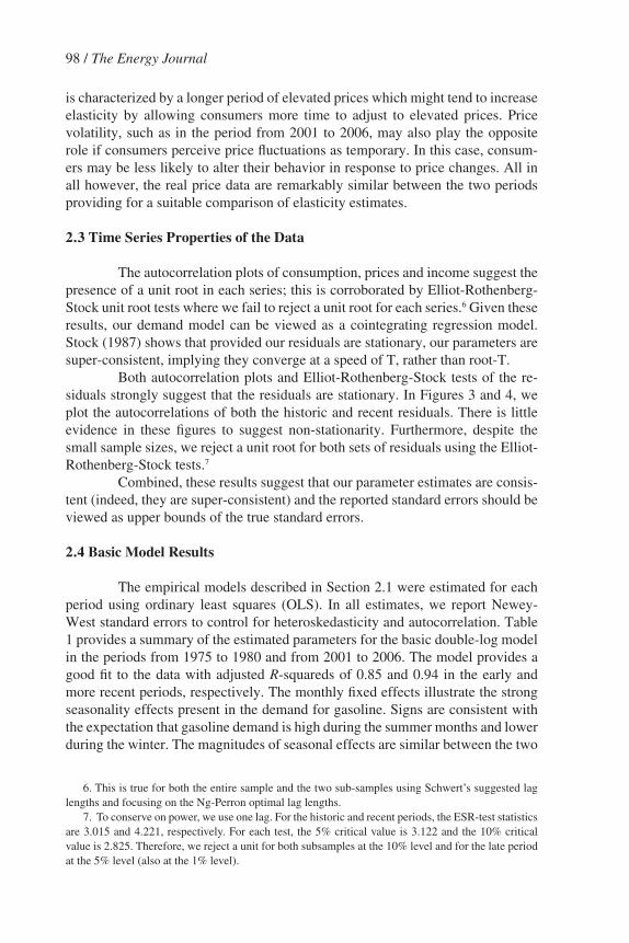
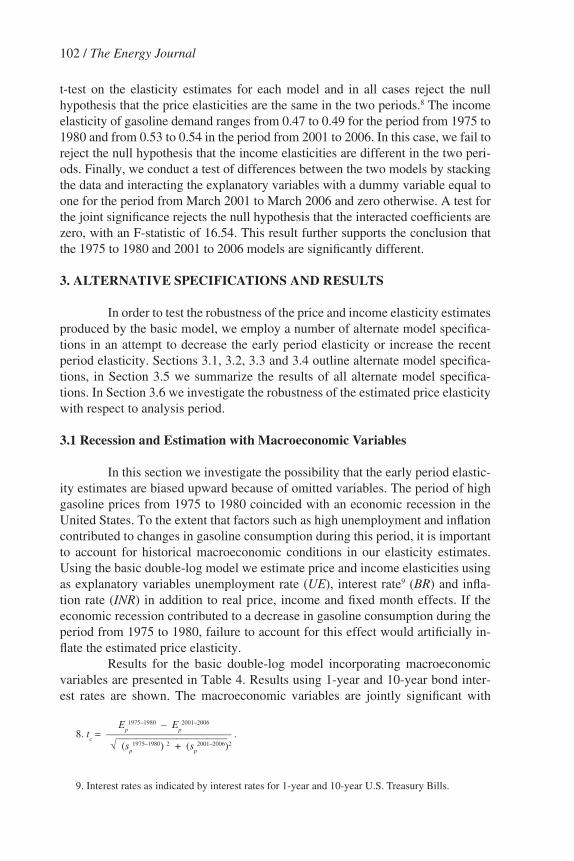
Both autocorrelation plots and Elliot-Rothenberg-Stock tests of the re-siduals strongly suggest that the residuals are stationary. In Figures 3 and 4, we plot the autocorrelations of both the historic and recent residuals. There is little evidence in these figures to suggest non-stationarity. Furthermore, despite the small sample sizes, we reject a unit root for both sets of residuals using the Elliot-Rothenberg-Stock tests.7

Combined, these results suggest that our parameter estimates are consis-tent (indeed, they are super-consistent) and the reported standard errors should be viewed as upper bounds of the true standard errors.

2.4 Basic Model Results

The empirical models described in Section 2.1 were estimated for each period using ordinary least squares (OLS). In all estimates, we report Newey-West standard errors to control for heteroskedasticity and autocorrelation. Table 1 provides a summary of the estimated parameters for the basic double-log model in the periods from 1975 to 1980 and from 2001 to 2006. The model provides a good fit to the data with adjusted R-squareds of 0.85 and 0.94 in the early and more recent periods, respectively. The monthly fixed effects illustrate the strong seasonality effects present in the demand for gasoline. Signs are consistent with the expectation that gasoline demand is high during the summer months and lower during the winter. The magnitudes of seasonal effects are similar between the two

6. This is true for both the entire sample and the two sub-samples using Schwert’s suggested lag lengths and focusing on the Ng-Perron optimal lag lengths.

7. To conserve on power, we use one lag. For the historic and recent periods, the ESR-test statistics are 3.015 and 4.221, respectively. For each test, the 5% critical value is 3.122 and the 10% critical value is 2.825. Therefore, we reject a unit for both subsamples at the 10% level and for the late period at the 5% level (also at the 1% level).


Figure 3. autocorrelation Plot for the Historic Residuals

Figure 4. autocorrelation Plot for the Recent Residuals


periods although the winter effect is somewhat smaller today than in the period from 1975 to 1980.

In Table 2, we present the results from two alternative functional forms alongside the double-log functional form. The monthly dummy variables have been excluded to simplify presentation of the results. The coefficients on price

table 1. olS Regression Results – Double-log Basic ModelBasic Model: Double log

1975 - 1980 2001 - 2006

bo -0.615 -1.697***

(0.929) (0.587)

ln(P) -0.335*** -0.042*** (0.024) (0.009)

ln(Y) 0.467*** 0.530*** (0.096) (0.058)

Jan -0.079*** -0.044*** (0.010) (0.006)

Feb -0.129*** -0.122*** (0.019) (0.010)

Mar -0.019*** -0.008 (0.006) (0.005)

Apr -0.021 -0.024*** (0.016) (-0.005)

May 0.013 0.026*** (0.011) (0.004)

Jun 0.020 0.000 (0.010) (0.004)

Jul 0.031*** 0.040*** (0.010) (0.005)

Aug 0.042*** 0.046*** (0.010) (0.004)

Sep -0.028*** -0.039*** (0.006) (0.005)

Oct 0.002 0.008 (0.010) (0.005)

Nov -0.058*** -0.032*** (0.012) (0.004)

ej’s y y

Adj. R-squared 0.85 0.94 S.E. of residuals 0.027 0.011 Durbin-Watson stat 1.762 1.520 Sum squared resid 0.033 0.006

Notes: Figures in parentheses are standard errors, *** (p < 0.01)

and income are significant (p < 0.01) for the basic model irrespective of functional form. Table 3 summarizes the average elasticities for the three models; estimates of the price elasticity of gasoline demand range from -0.31 to -0.34 in the period from 1975 to 1980 and from -0.041 to -0.043 in the period from 2001 to 2006. As-suming that the samples from each period are independent, we perform a Student’s


table 2. olS Regression Results – Basic ModelBasic Model

Basic Model: Basic Mode: Basic Model: linear Semi-log Double-log

1975-1980 2001-2006 1975-1980 2001-2006 1975-1980 2001-2006

bo 34.006 20.254 3.554 3.183 -0.615 -1.697

(3.868) (2.460) (0.098) (0.064) (0.929) (0.587)

P -7.252 -1.018 -0.180 -0.026 (0.554) (0.174) (0.013) (0.005)

Y 1.254E-03 7.943E-04 3.018E-05 2.035E-05 (2.633E-04) (9.862E-05) (6.536E-06) (2.567E-06)

ln (P) -0.335 -0.041 (0.024) (0.009)

ln (Y) 0.467 0.530 (0.096) (0.058)

ej’s y y y y y y

Adj. R-squared 0.85 0.94 0.85 0.94 0.85 0.94 S.E. of residuals 1.081 0.407 0.027 0.011 0.027 0.011 Durbin-Watson stat 1.721 1.591 1.729 1.582 1.762 1.520 Sum squared resid 54.925 7.794 0.0343 0.005 0.033 0.006

Notes: Figures in parentheses are standard errors, P is the real price of gasoline in constant 2000 dollars, Y is real per capita disposable income in constant 2000 dollars.

table 3. Price and Income Elasticities – Basic ModelBasic Model

1975-1980 2001-2006

Ep

Ei

Ep

Ei

tp

ti

Basic Model: Linear -0.312 0.487 -0.042 0.538 10.823 0.420 (0.024) (0.102) (0.007) (0.067)

Basic Mode: Semi-Log -0.309 0.471 -0.043 0.540 10.975 0.560 (0.023) (0.102) (0.007) (0.068)

Basic Model: Double-Log -0.335 0.467 -0.041 0.530 11.632 0.562 (0.024) (0.096) (0.009) (0.058)

Number of Observations = 61

Notes: Figures in parentheses are standard errors.


t-test on the elasticity estimates for each model and in all cases reject the null hypothesis that the price elasticities are the same in the two periods.8 The income elasticity of gasoline demand ranges from 0.47 to 0.49 for the period from 1975 to 1980 and from 0.53 to 0.54 in the period from 2001 to 2006. In this case, we fail to reject the null hypothesis that the income elasticities are different in the two peri-ods. Finally, we conduct a test of differences between the two models by stacking the data and interacting the explanatory variables with a dummy variable equal to one for the period from March 2001 to March 2006 and zero otherwise. A test for the joint significance rejects the null hypothesis that the interacted coefficients are zero, with an F-statistic of 16.54. This result further supports the conclusion that the 1975 to 1980 and 2001 to 2006 models are significantly different.

3. altERnatIvE SPEcIFIcatIonS anD RESultS

In order to test the robustness of the price and income elasticity estimates produced by the basic model, we employ a number of alternate model specifica-tions in an attempt to decrease the early period elasticity or increase the recent period elasticity. Sections 3.1, 3.2, 3.3 and 3.4 outline alternate model specifica-tions, in Section 3.5 we summarize the results of all alternate model specifica-tions. In Section 3.6 we investigate the robustness of the estimated price elasticity with respect to analysis period.

3.1 Recession and Estimation with Macroeconomic variables

In this section we investigate the possibility that the early period elastic-ity estimates are biased upward because of omitted variables. The period of high gasoline prices from 1975 to 1980 coincided with an economic recession in the United States. To the extent that factors such as high unemployment and inflation contributed to changes in gasoline consumption during this period, it is important to account for historical macroeconomic conditions in our elasticity estimates. Using the basic double-log model we estimate price and income elasticities using as explanatory variables unemployment rate (UE), interest rate9 (BR) and infla-tion rate (INR) in addition to real price, income and fixed month effects. If the economic recession contributed to a decrease in gasoline consumption during the period from 1975 to 1980, failure to account for this effect would artificially in-flate the estimated price elasticity.

Results for the basic double-log model incorporating macroeconomic variables are presented in Table 4. Results using 1-year and 10-year bond inter-est rates are shown. The macroeconomic variables are jointly significant with

Ep

1975–1980 – Ep

2001–2006

8. tc = ———————————— . ———————————

√ (sp

1975–1980) 2 + (sp

2001–2006)2

9. Interest rates as indicated by interest rates for 1-year and 10-year U.S. Treasury Bills.

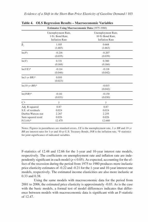
F-statistics of 12.48 and 12.66 for the 1-year and 10-year interest rate models, respectively. The coefficients on unemployment rate and inflation rate are inde-pendently significant in each model (p < 0.05). As expected, accounting for the ef-fect of the recession during the period from 1975 to 1980 produces more inelastic price elasticity estimates of -0.22 and -0.21 for the 1-year and 10-year interest rate models, respectively. The estimated income elasticities are also more inelastic at 0.33 and 0.38.

Using the same models with macroeconomic data for the period from 2001 to 2006, the estimated price elasticity is approximately -0.03. As is the case with the basic models, a formal test of model differences indicates that differ-ence between models with macroeconomic data is significant with an F-statistic of 12.47.


table 4. olS Regression Results – Macroeconomic variablesEstimates using Macroeconomic Data (1975-1980)

Unemployment Rate, Unemployment Rate, 1-Yr. Bond Rate, 10-Yr Bond Rate, Inflation Rate Inflation Rate

bo 1.105 0.668

(1.685) (1.663)

ln(P) -0.216 -0.207 (0.035) (0.039)

ln(Y) 0.331 0.380 (0.168) (0.166)

ln(UE)* -0.114 -0.118 (0.046) (0.042)

ln(1-yr BR)* 0.010 (0.023)

ln(10-yr BR)* -0.015 (0.042)

ln(INR)* -0.141 -0.130 (0.031) (0.030)

ej’s y y

Adj. R-squared 0.87 0.87 S.E. of residuals 0.024 0.024 Durbin-Watson stat 2.267 2.255 Sum squared resid 0.026 0.026 F(3,44)* 12.475 12.660

Notes: Figures in parentheses are standard errors, UE is the unemployment rate, 1-yr BR and 10-yr BR are interest rates for 1-yr and 10-yr U.S. Treasury Bonds, INR is the inflation rate, *F-statistics for joint significance of indicated variables.


3.2 Simultaneous Equations Models

A well-known problem in estimating demand equations occurs when price and quantity are jointly determined through shifts in both supply and de-mand resulting in biased and inconsistent parameter estimates. This problem is especially important when attempting to compare elasticity estimates between two periods. One potential explanation for the estimated elasticity differences is that the high prices of 1975 to 1980 were largely supply driven, while the high prices of 2001 to 2006 were demand driven; if this is the case, then our elastic-ity estimates for historic period will be unbiased, while our late-period elasticity estimates will be biased towards zero.

To address this concern, we instrument for price in the late period. An ideal instrumental variable for determining gasoline demand is one that is highly correlated with the price of gasoline (the endogenous variable) but not with unob-served shocks to gasoline demand. With respect to selection of instrumental vari-ables, Ramsey, Rasche and Allen (1975) and Dahl (1979) have used the relative prices of refinery products such as kerosene and residual fuel oil as instrumental variables. The problem with this approach is that the relative prices of other refin-ery outputs are likely to be correlated with gasoline demand shocks. Since gasoline demand and oil price are correlated, unobserved shocks to gasoline demand are likely to be correlated with the prices of other refinery outputs via the price of oil.

As it turns out, identifying appropriate instrumental variables for gaso-line demand is difficult. In this paper we experiment with crude oil production disruptions as instrumental variables.10 Disruptions are represented for three countries, Venezuela (VZ

jt), Iraq (IQ

jt) and the United States (US

jt). These three

countries were selected because each has had its production of crude oil affected by external shocks that are unlikely to be related to gasoline demand shocks. In Venezuela, a strike by oil workers beginning in December 2002 cut production to near zero and has significantly affected output for several years. In Iraq, an international embargo and more recently war have caused major disruptions to oil operations. In the United States, production has been in steady decline since the 1970s due to declining resources. In 2005, hurricanes Katrina and Rita resulted in the temporary loss of several hundred thousand barrels of production in the Gulf of Mexico.

For each country, crude oil production disruptions are defined by the dif-ference between actual production and a production forecast,11 for example VZ

jt =

production - forecast.12 The start of each disruption is defined by a specific event leading to a loss in production. In Venezuela, the disruption start corresponds

10. We also investigated crude oil quality as indicated by sulfur content and API specific gravity, however the coefficients on these variables were not significant in the first stage regression.

11. For forecasted oil production in each country we employ a simple double-log model using only a time trend and fixed month effects as explanatory variables.

12. In unreported results, we instead used a set of indicator variables representing the supply shocks. The results were qualitatively similar.

with the oil worker strike beginning in December of 2002 as reported by Banerjee (2002). In Iraq we use the beginning of the Second Gulf War in March of 2003 as reported by Tyler (2003). Finally, in the U.S., hurricane Katrina marks the begin-ning of the disruption reported by Mouawad and Bajaj (2005) in September 2005. The end of each disruption is defined as the month in which actual production reaches the forecasted production level. In the U.S., the forecast and production do not converge, but because production follows a highly seasonal pattern, the disruption end date is defined by the winter production peak marking the return to “normal” operations. Based on these definitions, the disruption periods are, December 2002 through March 2003 (VZ), March 2003 through November 2003 (IQ) and September 2005 through January 2006 (USA).

Using these instruments, we estimate Equation (1) via two-stage least squares (2SLS). Unfortunately, data on the instrumental variables are not avail-able for the entire study period. This prevents analysis of gasoline demand in the period from 1975 to 1980 using the instrumental variable approach. However, our goal is to determine if the elasticity differences we estimate are due to a bias in the later period estimates.

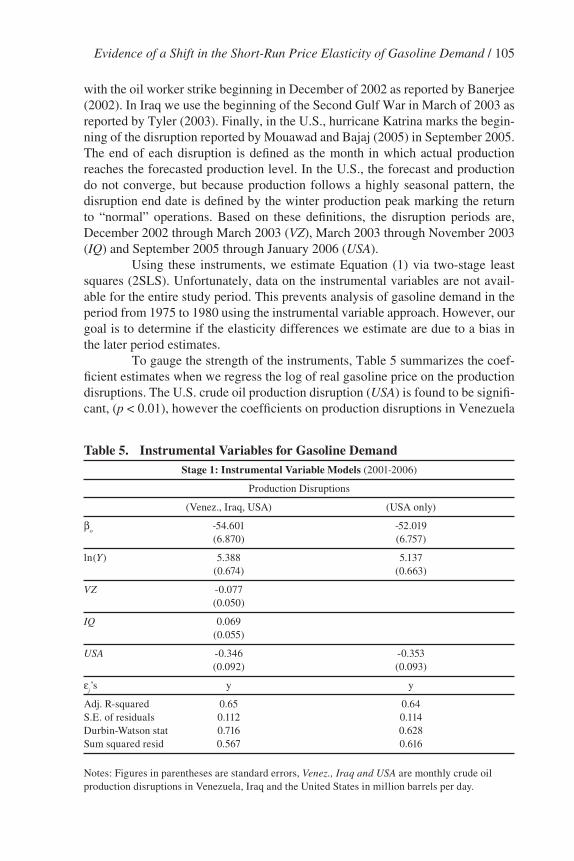
To gauge the strength of the instruments, Table 5 summarizes the coef-ficient estimates when we regress the log of real gasoline price on the production disruptions. The U.S. crude oil production disruption (USA) is found to be signifi-cant, (p < 0.01), however the coefficients on production disruptions in Venezuela


table 5. Instrumental variables for Gasoline DemandStage 1: Instrumental variable Models (2001-2006)

Production Disruptions

(Venez., Iraq, USA) (USA only)

bo -54.601 -52.019

(6.870) (6.757)

ln(Y) 5.388 5.137 (0.674) (0.663)

VZ -0.077 (0.050)

IQ 0.069 (0.055)

USA -0.346 -0.353 (0.092) (0.093)

ej’s y y


Notes: Figures in parentheses are standard errors, Venez., Iraq and USA are monthly crude oil production disruptions in Venezuela, Iraq and the United States in million barrels per day.


and Iraq are not significant (p = 0.13 and p = 0.22, respectively). Given these re-sults, we also report the results when using only disruptions in U.S. production.13

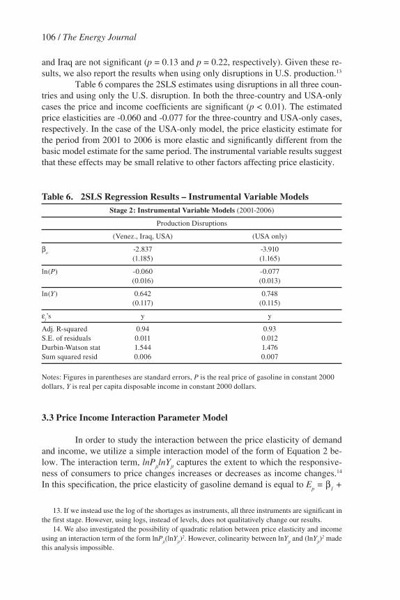
Table 6 compares the 2SLS estimates using disruptions in all three coun-tries and using only the U.S. disruption. In both the three-country and USA-only cases the price and income coefficients are significant (p < 0.01). The estimated price elasticities are -0.060 and -0.077 for the three-country and USA-only cases, respectively. In the case of the USA-only model, the price elasticity estimate for the period from 2001 to 2006 is more elastic and significantly different from the basic model estimate for the same period. The instrumental variable results suggest that these effects may be small relative to other factors affecting price elasticity.

3.3 Price Income Interaction Parameter Model

In order to study the interaction between the price elasticity of demand and income, we utilize a simple interaction model of the form of Equation 2 be-low. The interaction term, lnP

jtlnY

jt captures the extent to which the responsive-

ness of consumers to price changes increases or decreases as income changes.14 In this specification, the price elasticity of gasoline demand is equal to E

p = b

1 +

13. If we instead use the log of the shortages as instruments, all three instruments are significant in the first stage. However, using logs, instead of levels, does not qualitatively change our results.

14. We also investigated the possibility of quadratic relation between price elasticity and income using an interaction term of the form lnP

jt(lnY

jt)2. However, colinearity between lnY

jt and (lnY

jt)2 made

this analysis impossible.

table 6. 2SlS Regression Results – Instrumental variable Models Stage 2: Instrumental variable Models (2001-2006)

Production Disruptions

(Venez., Iraq, USA) (USA only)

bo -2.837 -3.910

(1.185) (1.165)

ln(P) -0.060 -0.077 (0.016) (0.013)

ln(Y) 0.642 0.748 (0.117) (0.115)

ej’s y y


Notes: Figures in parentheses are standard errors, P is the real price of gasoline in constant 2000 dollars, Y is real per capita disposable income in constant 2000 dollars.

b3lnY

jt. Since the price elasticity is less than zero, a positive coefficient b

3 on the

interaction term indicates a decrease in the price response as income rises.

lnGjt = b

o + b

1 lnP

jt + b

2 lnY

jt + b

3 lnP

jt lnY

jt + e

j + e

jt (2)

Results from OLS estimation of the price-income interaction model and partial-adjustment models are presented in Table 7 below. In the case of the price-income interaction model, the coefficients on price, income and the interaction term are significant for the period from 1975 to 1980 (p < 0.05) and for the period from 2001 to 2006 (p < 0.01).

3.4 Partial-adjustment Models

Another common approach to modeling gasoline demand is through the use of a partial-adjustment model. For example, see Houthakker, Verleger and


table 7. olS Regression Results – alternate SpecificationsPrice Income Interaction and Partial-adjustment Models

Partial-Adjustment Model: Price-Income 1-month Lag w/ Interaction Model Month Dummies

1975-1980 2001-2006 1975-1980 2001-2006

bo -12.755 -6.286 -0.467 -1.482

(6.094) (1.491) (0.838) (0.361)

ln(P) 27.572 10.297 -0.300 -0.033 (13.678) (3.223) (0.039) (0.005)

ln(Y) 1.720 0.981 0.409 0.390 (0.630) (0.146) (0.101) (0.033)

ln(P) ln(Y) -2.879 -1.014 (1.413) (0.316)

lnGt–1

0.107 0.330 (0.106) (0.074)

l 0.893 0.670

ej’s y y y y

Adj. R-squared 0.86 0.95 0.85 0.95 S.E. of residuals 0.026 0.010 0.027 0.010 Durbin-Watson stat 1.661 1.691 2.004 2.175 Sum squared resid 0.032 0.005 0.033 0.005 TR2

aux 28.635 18.569

Notes: Figures in parentheses are standard errors, P is the real price of gasoline in constant 2000 dollars, Y is real per capita disposable income in constant 2000 dollars, lnG

t–1 refers to 1-month

lags of the dependent variable, per capital gasoline consumption, TR2aux

is the test statistic for the Breusch-Godfrey Lagrange-Multiplier test for serial correlation.


Sheehan (1974). The partial-adjustment (PA) model is a dynamic model that in-cludes a lagged dependent variable. The rationale is that frictions in the market prevent reaching the appropriate equilibrium level and as a result, only a fraction of the desired change in consumption between periods is realized. In this section, we estimate a one-month partial-adjustment model. We use ln G

jt* in Equation 3

to represent the log of the equilibrium level of gasoline consumption. The realized consumption in month j and year t, lnG

jt is given by consumption in the previous

period, lnGjt-1

plus a fraction l (adjustment coefficient) of the difference between lnG

jt* and lnG

jt-1 as shown in Equation 4 below.

lnGjt* = b

o + b

1 lnP

jt + b

2 lnY

jt (3)

lnGjt = G

jt–1 + l(G

jt* – G

jt–1) + e

jt, 0 < l< 1 (4)

Substituting for lnGjt* in Equation 4 yields Equation 5 below which is

estimated by OLS. The short-run price and income elasticities are given by the coefficients x

2 and x

3, respectively. The fully-adjusted coefficients on the price

and income terms, x2,3

/ l= x2,3

/(1 – x1) are generally interpreted as long-run elas-

ticities. However, the interpretation is not as clear when monthly data are used. If the speed of adjustment (1/l) is relatively short, on the order of several months, the fully adjusted elasticities may also be interpreted as short-run. Both the short-run and fully-adjusted coefficients are reported for comparison.

lnGjt = x

o + x

1 G

jt–1 + x

2 lnP

jt + x

3 lnY

jt + e

jt (5)

The partial-adjustment models provide mixed results.15 For the period from 2001 to 2006, the coefficients on price, income and the lagged dependent variable are significant (p < 0.01) for both lag structures. For the period from 1975 to 1980, however, the coefficients on the lagged dependent variable and on income are not significant. With respect to the 2001 to 2006 results, the speed of adjustment is approximately 1.5 months. This suggests that the fully-adjusted elasticity estimates may be interpreted as short-run estimates and are included below for comparison. While the lagged-dependent variable is not significant in the historic period, the implied elasticities across the two time periods remain significantly different.

15. Because the Durbin-Watson test is not an appropriate test when lagged dependent variables are included as regressors, we perform a Breusch-Godfrey Lagrange-Multiplier (LM) test for serial correlation up to order 12 using TR2

aux as the test statistic. In the recent period, we fail to reject the null

hypothesis that the ρ’s are equal to zero, suggesting the presence of serial correlation in this model. In order to account for the downward bias that serial correlation would introduce into the standard error estimates, we use the Newey-West approach to calculate heteroskedasticity and autocorrelation consistent standard errors.

3.5 Summary of alternative Specifications Results

The estimated price and income elasticities of gasoline demand for al-ternate model specifications are summarized in Table 8 below. Based on the price income interaction, simultaneous equations and recession data models, the esti-mated price elasticity of gasoline demand is between -0.21 and -0.22 in the period from 1975 to 1980 and between -0.034 and -0.077 in the period from 2001 to 2006. While the partial-adjustment models do not provide a basis for comparison between the two periods, the estimated price and income elasticities in the period from 2001 to 2006 are consistent with other model specifications. A student’s t-test of the simultaneous equations and recession data model results shows that the estimated price elasticities in the two periods are significantly different (t = 3.15) even in the most conservative case.

3.6 Stability of the Estimated Price Elasticity over time

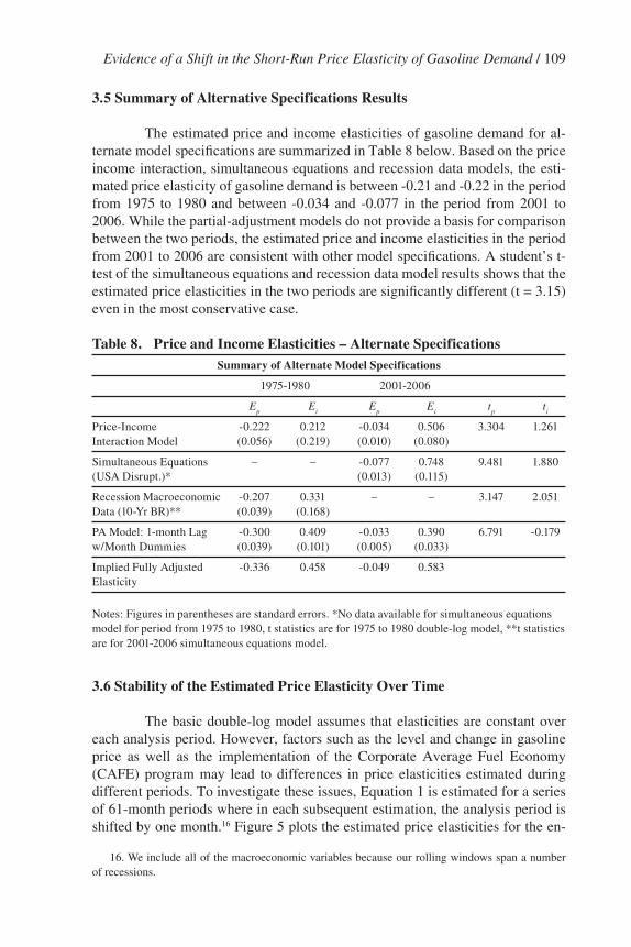
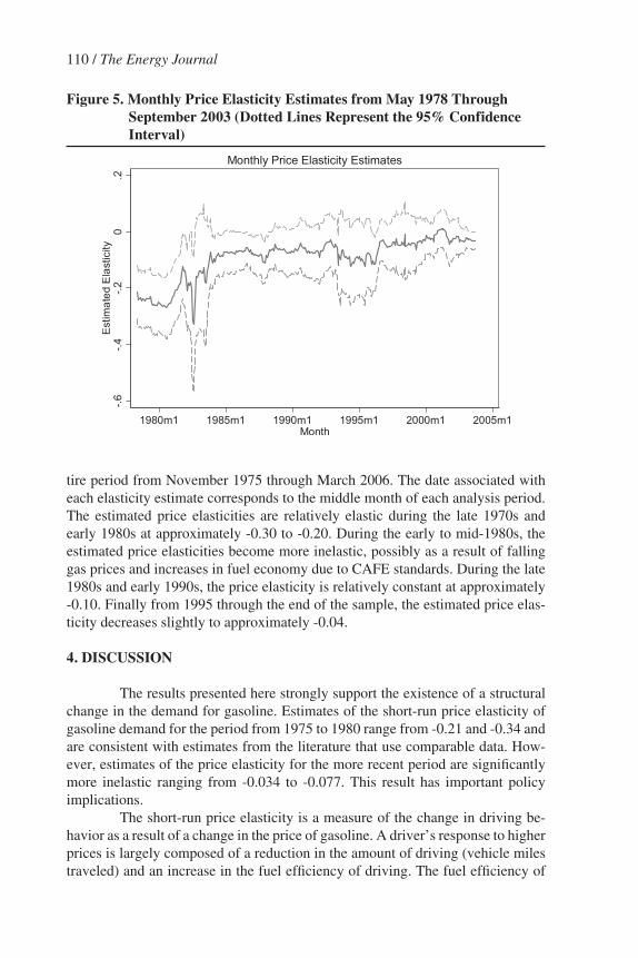
The basic double-log model assumes that elasticities are constant over each analysis period. However, factors such as the level and change in gasoline price as well as the implementation of the Corporate Average Fuel Economy (CAFE) program may lead to differences in price elasticities estimated during different periods. To investigate these issues, Equation 1 is estimated for a series of 61-month periods where in each subsequent estimation, the analysis period is shifted by one month.16 Figure 5 plots the estimated price elasticities for the en-

16. We include all of the macroeconomic variables because our rolling windows span a number of recessions.


table 8. Price and Income Elasticities – alternate SpecificationsSummary of alternate Model Specifications

1975-1980 2001-2006

Ep

Ei

Ep

Ei

tp

ti

Price-Income -0.222 0.212 -0.034 0.506 3.304 1.261 Interaction Model (0.056) (0.219) (0.010) (0.080)

Simultaneous Equations – – -0.077 0.748 9.481 1.880 (USA Disrupt.)* (0.013) (0.115)

Recession Macroeconomic -0.207 0.331 – – 3.147 2.051 Data (10-Yr BR)** (0.039) (0.168)

PA Model: 1-month Lag -0.300 0.409 -0.033 0.390 6.791 -0.179 w/Month Dummies (0.039) (0.101) (0.005) (0.033)

Implied Fully Adjusted -0.336 0.458 -0.049 0.583 Elasticity

Notes: Figures in parentheses are standard errors. *No data available for simultaneous equations model for period from 1975 to 1980, t statistics are for 1975 to 1980 double-log model, **t statistics are for 2001-2006 simultaneous equations model.


tire period from November 1975 through March 2006. The date associated with each elasticity estimate corresponds to the middle month of each analysis period. The estimated price elasticities are relatively elastic during the late 1970s and early 1980s at approximately -0.30 to -0.20. During the early to mid-1980s, the estimated price elasticities become more inelastic, possibly as a result of falling gas prices and increases in fuel economy due to CAFE standards. During the late 1980s and early 1990s, the price elasticity is relatively constant at approximately -0.10. Finally from 1995 through the end of the sample, the estimated price elas-ticity decreases slightly to approximately -0.04.

4. DIScuSSIon

The results presented here strongly support the existence of a structural change in the demand for gasoline. Estimates of the short-run price elasticity of gasoline demand for the period from 1975 to 1980 range from -0.21 and -0.34 and are consistent with estimates from the literature that use comparable data. How-ever, estimates of the price elasticity for the more recent period are significantly more inelastic ranging from -0.034 to -0.077. This result has important policy implications.

The short-run price elasticity is a measure of the change in driving be-havior as a result of a change in the price of gasoline. A driver’s response to higher prices is largely composed of a reduction in the amount of driving (vehicle miles traveled) and an increase in the fuel efficiency of driving. The fuel efficiency of

Figure 5. Monthly Price Elasticity Estimates from May 1978 through September 2003 (Dotted lines Represent the 95% confidence Interval)

driving can be increased through for example, improved vehicle maintenance or changes in driving behavior such as slower acceleration or reduced vehicle speed. In addition, shifts in household vehicle stock utilization may contribute to short-run elasticity. The short-run elasticity may also include more permanent changes in the vehicle stock (e.g. the purchase of more fuel efficient vehicles), though vehicle purchase decisions are typically regarded as more long-run in nature. The results presented here suggest that on average, U.S. drivers appear less responsive in adjusting to gasoline price increases than in previous decades.

It may be the case that today’s U.S. consumers are more dependent on automobiles for daily transportation than during the 1970s and 1980s and as a re-sult, are less able to reduce vehicle miles traveled in response to higher prices. One hypothesis is that an increase in suburban development has led to larger distances between travel destinations. This could mean that drivers have less ability to re-spond to price changes because greater distances decrease the viability of non-mo-torized modes such as walking or biking. In addition, when development patterns increase the distance between home and non-discretionary destinations such as the workplace, a greater share of the total vehicle miles traveled are fixed. An increase in multiple income households would further decrease flexibility if a greater share of the population requires a daily work commute. Finally, these effects are com-pounded if the availability of public transit is less than in earlier decades.

Another hypothesis is that as incomes have grown, the budget share rep-resented by gasoline consumption has decreased making consumers less sensitive to price increases. The price income interaction model presented here provides insight into this hypothesis. If increasing income results in a decrease in the con-sumer response to gasoline price changes, one would expect the coefficient on the interaction term of the model to have a positive sign. However, in both periods we find that the coefficient on the interaction term is negative suggesting that on average, gasoline consumption is more sensitive to price changes as income rises. This somewhat counterintuitive result is supported by the household gasoline de-mand analysis conducted by Kayser (2000) who also finds a negative coefficient on the price income interaction term.17 The hypothesis proposed by Kayser is that as incomes rise, a greater proportion of automobile trips are discretionary. Alter-natively, at lower income levels, the amount of travel has already been reduced to the minimum leaving little room for adjustment to higher prices. Another possible explanation is that the number of vehicles per household increases with income. When the number of household vehicles exceeds the number of drivers, there is the possibility for drivers to shift to more fuel efficient vehicles within the house-hold stock as gasoline prices rise. Whatever the explanation, the overall decrease in price elasticity despite growth in incomes suggests that these effects are rela-tively minor compared to other factors affecting gasoline demand.

17. Small and Van Dender (2007) find that increases in income reduce the rebound effect, in contrast to our results. There are two potential reasons for this difference. For one, our data are aggregate in nature. Second, by splitting the entire series into two time periods, the large income swings between the 1970s and 2000s are captured by changes in the intercept.



Finally, the overall improvement in U.S. fleet average fuel economy since the late 1970s and early 1980s may have also contributed to a decrease in the re-sponsiveness of consumers to gasoline price increases. Largely a result of the U.S. Corporate Average Fuel Economy (CAFE) and market penetration of fuel efficient foreign vehicles during the period, the U.S. fleet average fuel economy improved from approximately 15 miles per gallon in 1980 to approximately 20 miles per gallon in 2000 according to National Research Council (2002). Because the ve-hicle fleet has become more fuel efficient, a decrease in miles traveled today has a smaller impact on gasoline consumption. That is to say if for example discretion-ary travel is reduced, the resulting reduction in gasoline consumption today is less than in 1980 because today’s vehicles consume less fuel per mile driven.

The results presented in Section 3.6 provide some clues about the poten-tial causes of the shift in price elasticity we observe. The largest change occurs over a relatively short period of three to four years during the early 1980s. The remaining years show a gradual decrease in the price elasticity. Since factors such as changes in land-use and transit infrastructure typically take place over many years, these types of changes may contribute to the gradual change in elasticity observed in Section 3.6. On the other hand, the rapid change during the early 1980s may be the result of the CAFE program and other factors which caused relatively quick changes in fleet average fuel economy during that period.

Whatever the cause, the results presented here suggest that today’s consum-ers have not significantly altered their gasoline consumption in response to higher gasoline prices. It is important to note that these results measure consumers’ reac-tions to short-run changes in gasoline prices. However, it is the long-run response that is the most important in determining which polices are most appropriate for reducing gasoline consumption. As it turns out, it is relatively difficult to measure long-run gasoline elasticities in practice due to factors such as the cyclical nature of gasoline prices. In this paper, we are also limited to currently available data and the relatively short history of high gasoline prices during the past several years.

Analysis of the short-run price elasticity does however provide some in-sight into long-run behavior. The long-run response to gasoline price increases is the sum of short-run changes (miles driven) and long-run changes (fuel economy of the vehicle fleet). The short-run results suggest that consumers today are less responsive in adjusting miles driven to increases in gasoline price. This compo-nent seems unlikely to change significantly for long-run behavior. This is because factors that may contribute to inelastic short-run price elasticities such as land use, employment patterns and transit infrastructure typically evolve on timescales greater than those considered in long-run decisions.

In terms of vehicle fuel economy, consumers may respond to higher gas-oline prices in the long-run by purchasing more fuel efficient vehicles. However, if consumers in the period from 2001 to 2006 were purchasing more fuel efficient vehicles in response to higher gasoline prices, one would expect to see at least a portion of this effect in the short-run elasticity. While our results do not preclude a significant shift to more fuel efficient vehicles in the long-run response, the highly

inelastic values that we observe suggest that the vehicle fuel economy component is small. If the long-run price elasticity is in fact more inelastic than in previous decades, smaller reductions in gasoline consumption will occur for any given gasoline tax level. As a result, a tax would need to be significantly larger today in order to achieve an equivalent reduction in gasoline consumption. In the U.S., gasoline taxes have been politically difficult to implement. Higher required tax levels pose an addition hurdle. This may make tax policies impossible to imple-ment in practice. In this case, alternate measures such as increases in the CAFE standard may be required to achieve desired reductions in gasoline consumption.

5. SuMMaRy anD concluSIonS

In this paper we estimate the average per capita demand for gasoline in the U.S. for the period from 1974 to 2006. We investigate two periods of similar gasoline price increases in order to compare the demand elasticities in the 1970s and 1980s with today. We find that the short-run price elasticity of U.S. gasoline demand is significantly more inelastic today than in previous decades. This result is robust and consistent across several empirical models and functional forms. The observed change provides evidence of a structural change in the U.S. market for transportation fuel and may reflect shifts in land-use, social or vehicle characteris-tics during the past several decades. Provided our results extend to long-run elastic-ities, these results suggest that technologies and policies for improving vehicle fuel economy may be increasingly important in reducing U.S. gasoline consumption.

6. REFEREncES

Banerjee, N. (2002). “Venezuela Strife Pushes Crude Oil to $30.” The New York Times. Late Edition - Final. C 1. December 17, 2002.

Bureau of Economic Analysis, “National Economic Accounts, Implicit Price Deflators for Gross Do-mestic Product”. Accessed May 19, 2006. http://www.bea.gov/bea/dn/nipaweb/index.asp.

Bureau of Economic Analysis, “National Economic Accounts, Personal Income and Its Disposition”. U.S. Department of Commerce. Accessed May 19, 2006. http://www.bea.gov/bea/dn/nipaweb/index.asp.

Dahl, C. and T. Sterner (1991). “Analyzing Gasoline Demand Elasticities: A Survey.” Energy Eco-nomics 3(13): 203-210.

Dahl, C. A. (1979). “Consumer Adjustment to a Gasoline Tax.” The Review of Economics and Sta-tistics 61(3): 427-432.

Elliott, G., T.J. Rothenberg and J.H. Stock (1996). “Efficient Tests for an Autoregressive Unit Root.” Econometrica 64(4): 813-836.

Espey, M. (1996). “Explaining the Variation in Elasticity Estimates of Gasoline Demand in the United States: A Meta-Analysis.” The Energy Journal 17(3): 49-60.

Espey, M. (1998). “Gasoline Demand Revisited: An International Meta-Analysis of Elasticities.” En-ergy Economics 20: 273-295.

Houthakker, H. S., P. K. Verleger and D. P. Sheehan (1974). “Dynamic Demand Analysis for Gaso-line and Residential Electricity.” American Journal of Agricultural Economics 56(2): 412-418.

Hsing, Y. (1990). “On the Variable Elasticity of the Demand for Gasoline.” Energy Economics 12(2): 132-136.

Kahn, M. E. (2000). “The Environmental Impact of Suburbanization.” Journal of Policy Analysis and Management 19(4): 569-586.



Kayser, H. A. (2000). “Gasoline Demand and Car Choice: Estimating Gasoline Demand Using House-hold Information.” Energy Economics 22(3): 331-348.

Mouawad, J. and V. Bajaj (2005). “Gulf Oil Operations Remain in Disarray.” The New York Times. Late Edition - Final. C 1. September 2, 2005.

National Research Council, (2002). “Effectiveness and Impact of Corporate Average Fuel Economy (CAFE) Standards.” National Academy Press.

Ng, S. and P. Perron (2001). “Lag Length Selection and the Construction of Unit Root Tests with Good Size and Power.” Econometrica 69(6): 1519-1554.

Nicol, C. J. (2003). “Elasticities of Demand for Gasoline in Canada and the United States.” Energy Economics 25(2): 201-214.

Polzin, S. E. and X. Chu (2005). “A Closer Look at Public Transportation Mode Share Trends.” Jour-nal of Transportation and Statistics 8(3): 41-53.

Puller, S. L. and L. A. Greening (1999). “Household Adjustment to Gasoline Price Change: An Analy-sis Using 9 Years of U.S. Survey Data.” Energy Economics 21(1): 37-52.

Ramsey, J., R. Rasche and B. Allen (1975). “An Analysis of the Private and Commercial Demand for Gasoline.” The Review of Economics and Statistics 57(4): 502-507.

Schmalensee, R. and T. M. Stoker (1999). “Household Gasoline Demand in the United States.” Econometrica 67(3): 645-662.

Schwert, W. G. (1989). “Test for Unit Roots: A Monte Carlo Investigation.” Journal of Business and Economic Statistics 7(2): 147-160.

Small, K. A. and K. Van Dender (2007). “Fuel Efficiency and Motor Vehicle Travel: The Declining Rebound Effect.” The Energy Journal 28(1): 25-51.

Stock, J. H. (1987). “Asymptotic Properties of Least Squares Estimators of Cointegrating Vectors.” Econometrica 55(5): 1035-1056.

Tyler, P. E. (2003). “A Nation at War: The Attach; U.S. And British Troops Push into Iraq as Missles Strike Baghdad Compound.” The New York Times. Late Edition - Final. A 1. March 21, 2003.

U.S. Bureau of Labor Statistics, “Bureau of Labor Statistics Data, Prices and Living Conditions”. U.S. Department of Labor. Accessed May 15, 2006. http://www.bls.gov/data/home.htm.

U.S. Bureau of Labor Statistics, “Labor Force Statistics from the Current Population Survey”. U.S. Department of Labor. Accessed August 25, 2006. http://data.bls.gov/PDQ/outside.jsp?survey=ln.

U.S. Energy Information Administration, “International Petroleum Monthly, World Crude Oil Produc-tion”. U.S. Department of Energy. Accessed July 26, 2006. www.eia.doe.gov/emeu/ipsr/t11c.xls.

U.S. Energy Information Administration, “Petroleum Navigator, Supply and Disposition”. U.S. De-partment of Energy. Accessed May 15, 2006. http://tonto.eia.doe.gov/dnav/pet/pet_sum_snd_c_nus_epm0f_mbbl_m.htm.

U.S. Federal Reserve Board, “Federal Reserve Statistical Release, Selected Interest Rates”. U.S. Federal Reserve Board. Accessed August 24, 2006. http://www.federalreserve.gov/RELEASES/h15/data.htm.

aPPEnDIx – altERnatIvE SPEcIFIcatIonS Data

Additional data used in the alternative model specifications are defined as follows. The monthly crude oil production for Venezuela, Iraq and the United States are monthly average production in million barrels per day from the International Petroleum Monthly, U.S. Energy Information Administration (2006). Unemployment rates are U.S. aggregate for citizens over the age of 16 from the U.S. Bureau of Labor Statistics (2006). Interest rates are for 1-year and 10-year U.S. Treasury Bills (constant maturities) as cited by the U.S. Federal Reserve Board (2006). Per capita quantities are calculated using mid-period monthly population from the Bureau of Economic Analysis (2006).

Documents

Evidence of a Shift in the Short-Run Price Elasticity of