Evidence for Anisotropy and Intermittency in the Turbulent Interstellar Plasma

Bill Coles, University of California, San Diego

1. It had been thought that turbulence in the WIM was more or less isotropic. This view was based on a few VLBI observations of highly scattered sources. However highly scattered sources are atypical. Evidence is accumulating that anisotropy may be actually relatively common.

2. There is no doubt that the warm interstellar plasma (WIM) is highly sporadic, but it is not clear that it is intermittent in the sense used in hydrodynamics. However the tiny structures observed by Dan and discussed by Barney may be evidence for intermittency.

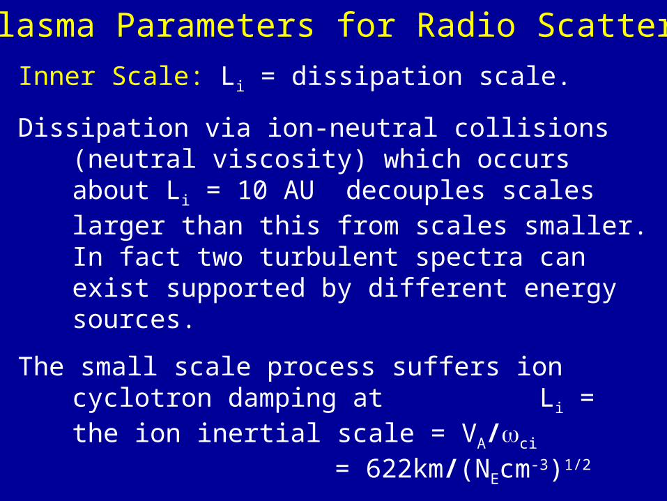
Key Plasma Parameters for Radio Scattering

Inner Scale: Li = dissipation scale.

Dissipation via ion-neutral collisions (neutral viscosity) which occurs about Li = 10 AU decouples scales larger than this from scales smaller. In fact two turbulent spectra can exist supported by different energy sources.

The small scale process suffers ion cyclotron damping at Li = the ion inertial scale = VA/ci

= 622km/(NEcm-3)1/2

Thermal pressure/Magnetic pressure: = NEkT/B2

< 1 -> magnetic fields dominate -> anisotropy likely

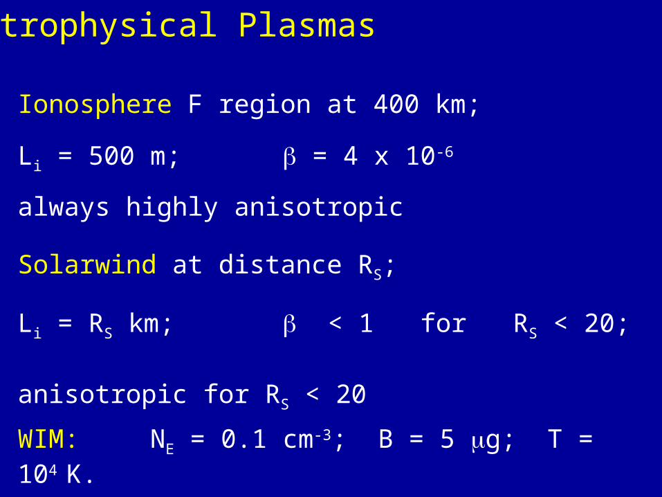
Astrophysical Plasmas

Ionosphere F region at 400 km;

Li = 500 m; = 4 x 10-6

always highly anisotropic

Solarwind at distance RS;

Li = RS km; < 1 for RS < 20;

anisotropic for RS < 20

WIM: NE = 0.1 cm-3; B = 5 g; T = 104 K.

Li = 2200 km; = 0.15

Solar Wind Anisotropy vs Solar Distance

Model AR(R) of plasma

expected AR(R) for radio wave

The vertical bars indicate variation not statistical error

< 1 > 1

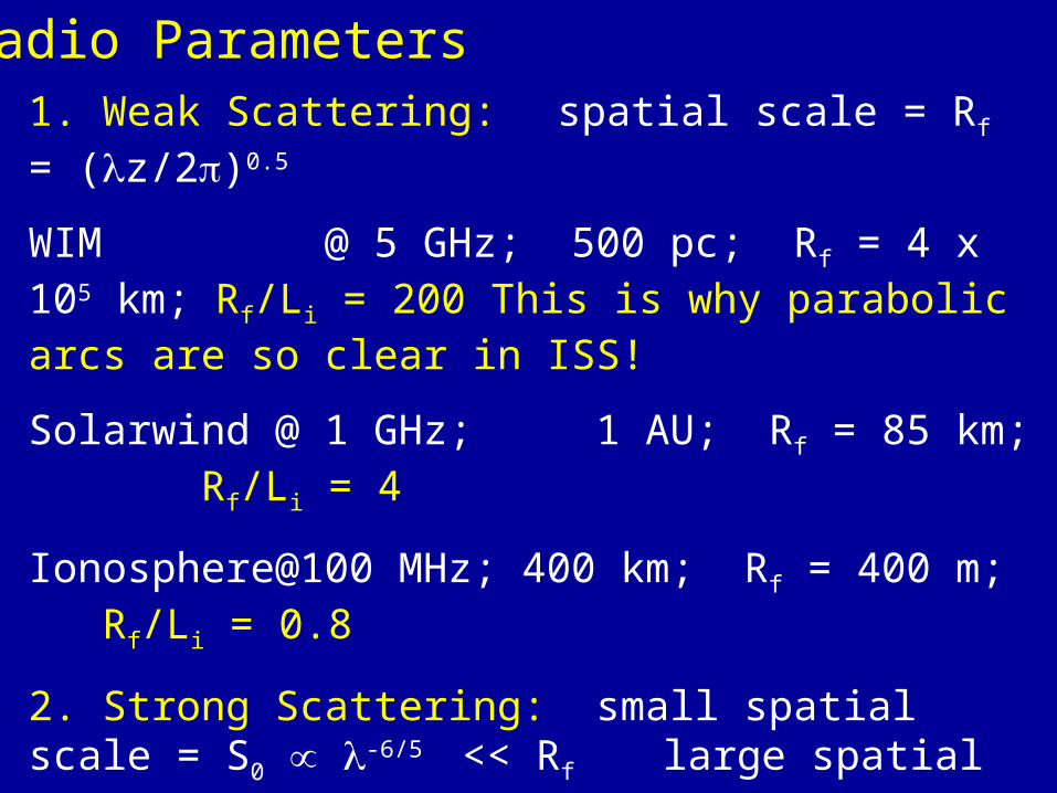
Radio Parameters1. Weak Scattering: spatial scale = Rf = (z/2)0.5

WIM @ 5 GHz; 500 pc; Rf = 4 x 105 km; Rf/Li = 200 This is why parabolic arcs are so clear in ISS!

Solarwind @ 1 GHz; 1 AU; Rf = 85 km; Rf/Li = 4

Ionosphere@100 MHz; 400 km; Rf = 400 m; Rf/Li = 0.8

2. Strong Scattering: small spatial scale = S0 -6/5 << Rf

large spatial scale = SR where SRS0=Rf2

WIM 100 MHz; S0/Li = 2; so arcs are always visible

SR = 4 x 107 km, so even the largest scales remain below the ion-neutral cutoff scale.

More Radio Parameters

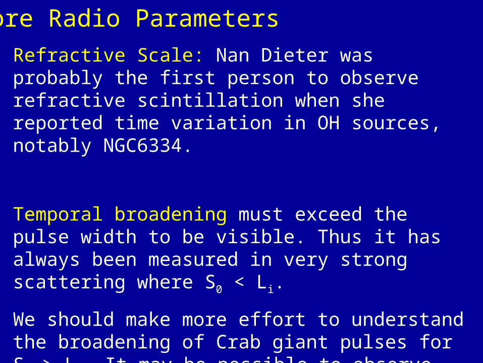
Refractive Scale: Nan Dieter was probably the first person to observe refractive scintillation when she reported time variation in OH sources, notably NGC6334.

Temporal broadening must exceed the pulse width to be visible. Thus it has always been measured in very strong scattering where S0 < Li.

We should make more effort to understand the broadening of Crab giant pulses for S0 > Li. It may be possible to observe temporal broadening in the inertial subrange.

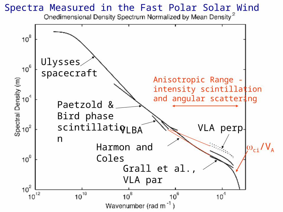
Ulyssesspacecraft

VLBA

Grall et al., VLA par

Harmon and Coles

Paetzold & Bird phase scintillation

VLA perp

ci/VA

Anisotropic Range -intensity scintillationand angular scattering

Spectra Measured in the Fast Polar Solar Wind

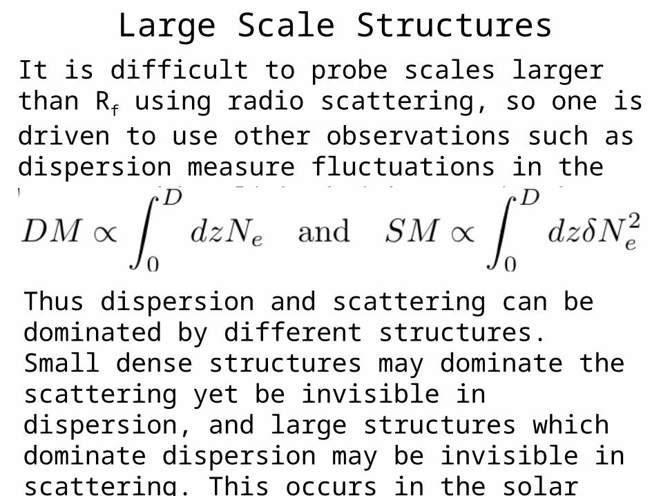
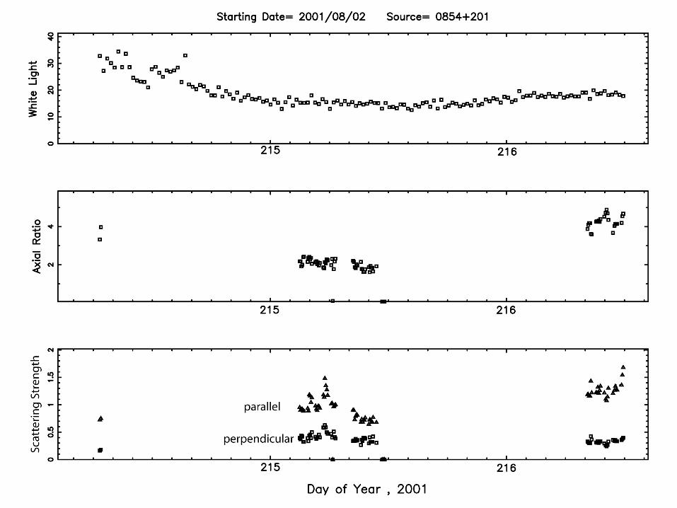
Large Scale StructuresIt is difficult to probe scales larger than Rf using radio scattering, so one is driven to use other observations such as dispersion measure fluctuations in the WIM, or white light brightness in the Solar corona. However

Thus dispersion and scattering can be dominated by different structures. Small dense structures may dominate the scattering yet be invisible in dispersion, and large structures which dominate dispersion may be invisible in scattering. This occurs in the solar wind, and probably in the WIM

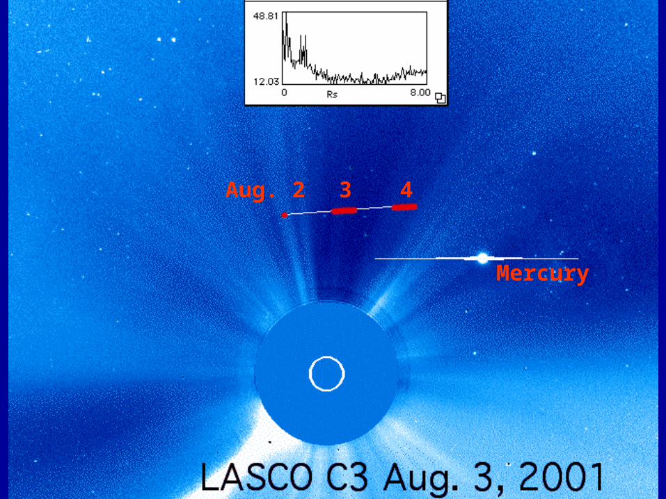
Aug. 2 3 4

Mercury

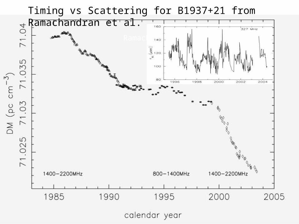
Ramachandran et al 2006:

Timing vs Scattering for B1937+21 from Ramachandran et al.

Anisotropy

It is hard to measure anisotropy in the WIM directly because the spatial scales are much larger than our interferometers unless the scattering is very strong. Of course very strong scattering implies more distant pulsars and less likelihood of the scattering being dominated by a single compact region.

There are two indirect methods which work in relatively weak scattering: (1) intensity correlations; (2) the secondary spectrum.

1. The shape of the auto-correlation in weak-scattering becomes very angle-dependent when the medium is anisotropic.

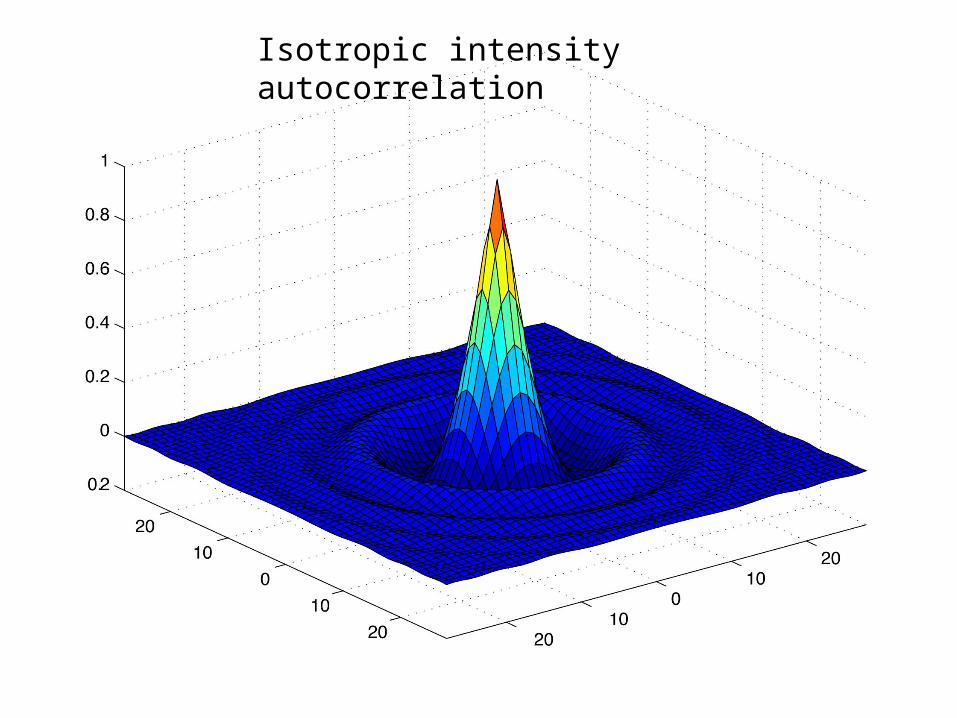
Isotropic intensity autocorrelation

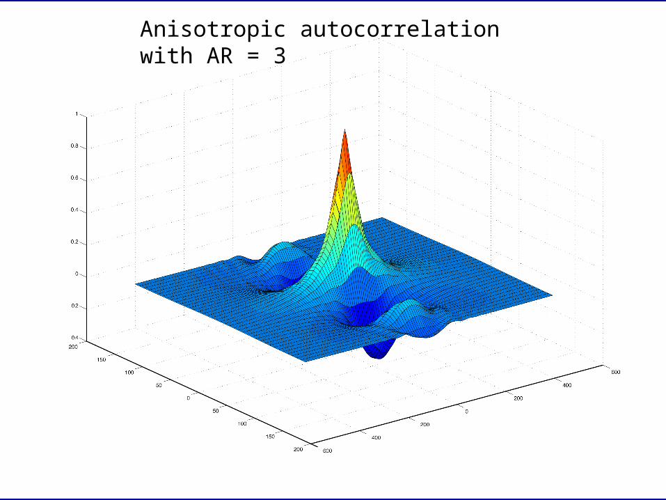
Anisotropic autocorrelation with AR = 3

Observational Evidence

There are several ways one can make use of this correlation.

1. If a cut through the intensity correlation shows strong oscillation then the AR > 3 is likely.

2. If the system cuts through the correlation at different angles then the time constant will change with angle. This occurs in two situations: (a) due to changes in the Earth’s velocity; (b) due to changes in the pulsar velocity.

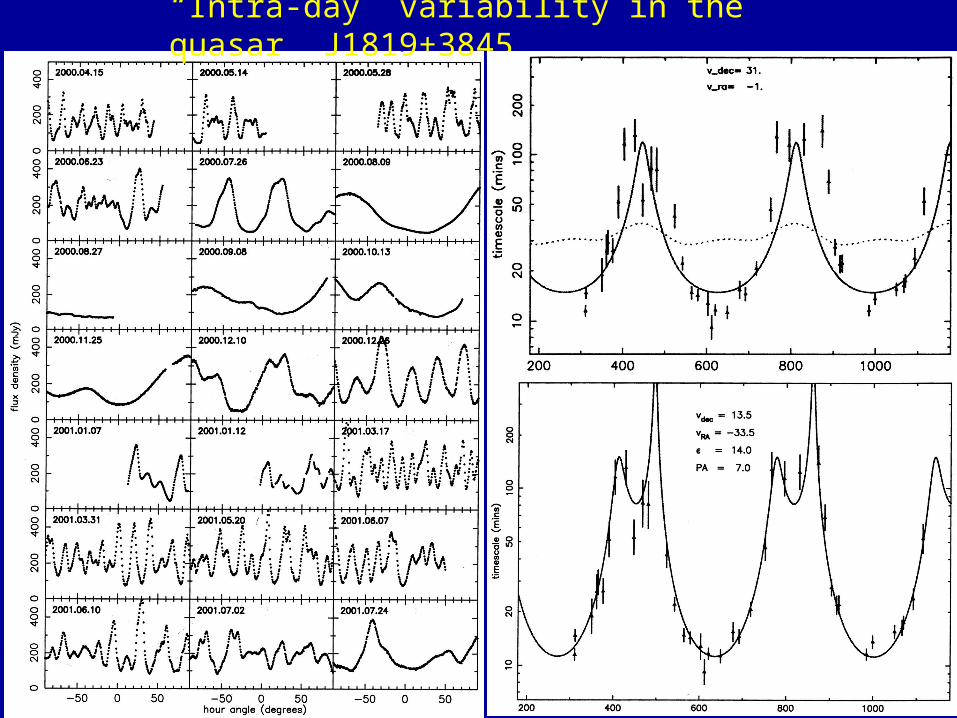
“Intra-day” variability in the quasar J1819+3845

Secondary Spectra

Secondary spectra provide even more direct evidence for anisotropy. In weak scattering the secondary spectrum can actually be inverted to obtain the two-dimensional phase spectrum, so anisotropy can be observed directly. In strong scattering an inversion is not possible but the effect of anisotropy is clear.

This is best seen on full-electromagnetic simulations.

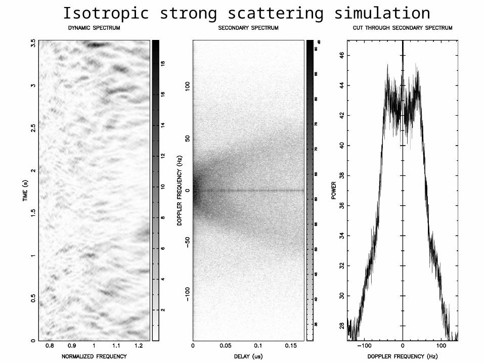
Isotropic strong scattering simulation

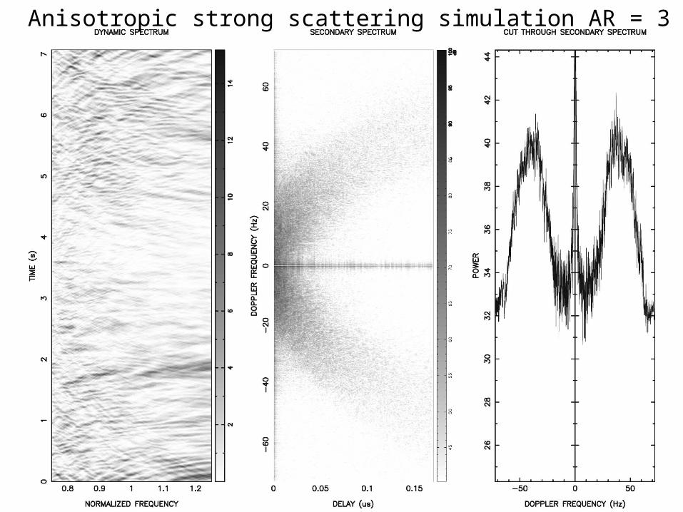
Anisotropic strong scattering simulation AR = 3

Why do we care about anisotropy anyway?

So we have evidence that anisotropy is more common than had been thought. So what?

1. Analysis of IDV and binary pulsar observations depends strongly on anisotropy and failure to include it will lead to serious errors.

2. Observation of anisotropic turbulence suggests that the plasma < 1, which may provide an interesting bound on the magnetic field and/or the temperature.

3. The refractive scale size is considerably larger when the turbulence is anisotropic. The simple concept of the “scattering disc” = “refractive scale” breaks down.

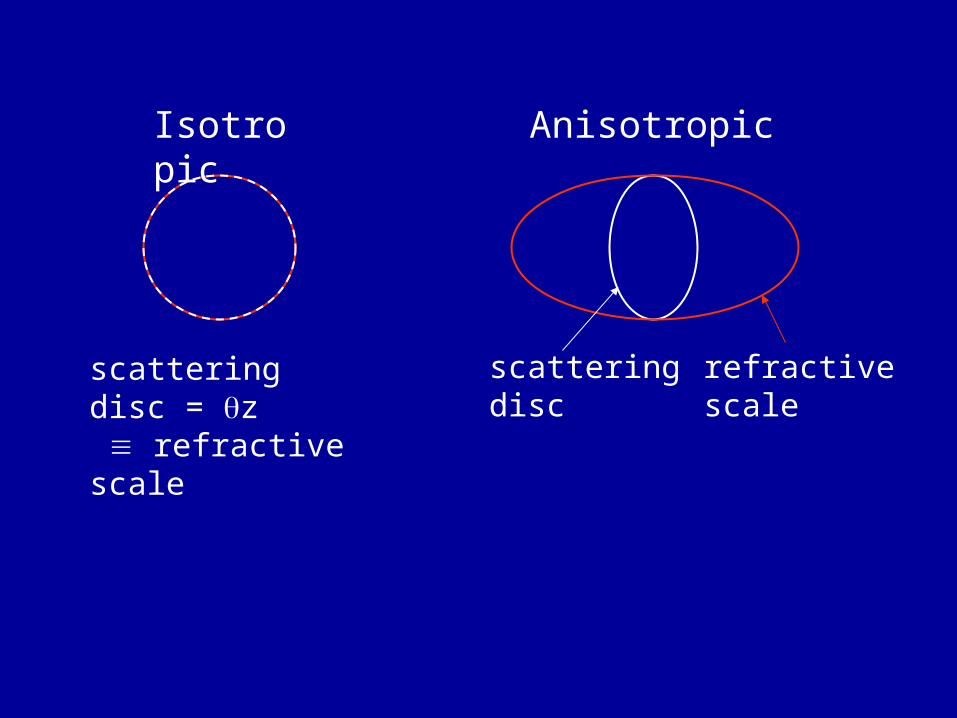
Isotropic Anisotropic

scatteringdisc

refractivescale

scattering disc = z refractive scale

Spatial Variation in Level of Turbulence

Scattering observations of different pulsars, even close neighbours, show radically different scattering strengths. This can be seen most directly in a plot of the effective pulse broadening vs dispersion measure.

Spatial Variations of Level of TurbulenceOne can model this variation using a random population of pc sized structures with Ne = 0.1 to 10 cm-3. The mean separation needed is 10’s of pc.

These objects are large compared with the scattering disc and the drift time is very long. However they are small compared with the distance to the Earth - thus they can be modeled by a Thin Screen, and they will show arcs.

Secondary spectra show well-defined arcs which persist for decades apparently unchanged. Sometimes they show several persistent well-defined arcs, suggesting that several scattering objects may be involved.

Double Pulsar ScintillationsStrong scattering spatial scale = 40,000 km @ 1400 MHz Rf = 5.6 x 105 km; Scattering disc = 2 x 107 km; drift time for scattering disc = 8 days; Orbital period = 2.4 hrs. Orbital diameter = 9 x 105 km -> during an orbit one does not see refractive scintillation.

Phase gradients are obvious at some times but not at others. The gradient must persist for at least 2 x 107 km but cannot last longer than 108 km. They cause asymmetrical arcs.

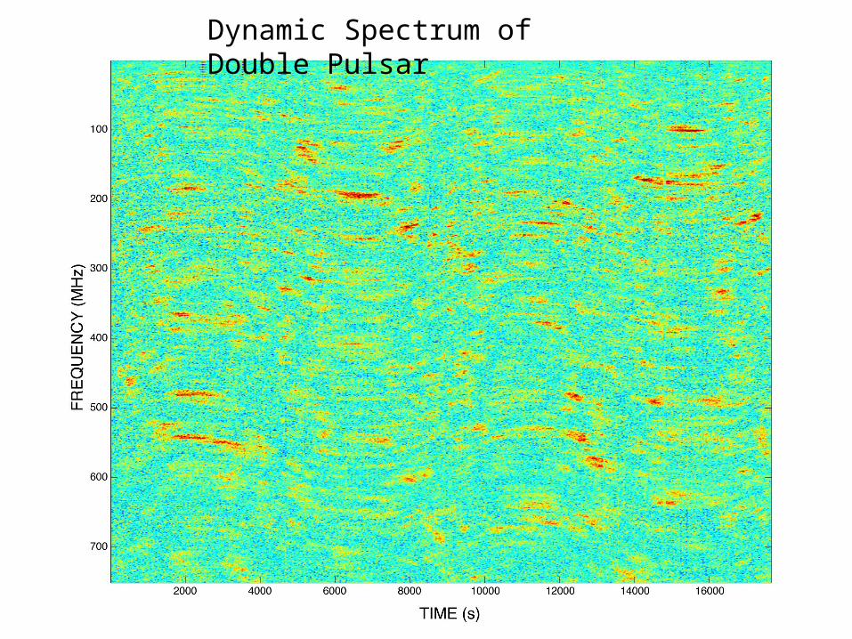
Dynamic Spectrum of Double Pulsar

We thought that these gradients required an excess of phase over a Kolmogorov spectrum and might be related to Tiny Structures. However we (recently) have been able to simulate them with a Kolmogorov spectrum - alas.

So these phase gradients are unremarkable…

IntermittencyHowever secondary spectra also show much smaller structures which cross the line of sight on a time scale of months. There is also evidence for such structures in the ISS of extra-galactic IDV sources.

These Tiny Structures have sub-AU diameters, yet they must be common. It is reasonable to imagine that they are “intermittent plumes” of turbulence within the pc-sized structures.

A suitable generating mechanism might be the shear-instabilities. Colliding clouds would certainly generate such plumes close to the contact surface, and they would stop growing in size and persist as “fossil” plumes after the clouds moved apart.