Evidence for a probabilistic, brain-distributed, recursive ... · Evidence for a probabilistic, brain-distributed, recursive mechanism for decision-making Javier A. Caballero 1 ;

Evidence for a probabilistic, brain-distributed, recursive mechanism fordecision-making

Javier A. Caballero1,2,3, Mark D. Humphries 1,4, Kevin N. Gurney 2,4

Abstract

Decision formation recruits many brain regions, but the procedure they jointly execute is unknown. Tocharacterize it, we introduce a recursive Bayesian algorithm that makes decisions based on spike trains. Using it tosimulate the random-dot-motion task, based on area MT activity, we demonstrate it quantitatively replicates thechoice behaviour of monkeys, whilst predicting losses of usable sensory information. Its architecture maps to therecurrent cortico-basal-ganglia-thalamo-cortical loops, whose components are all implicated in decision-making.We show that the dynamics of its mapped computations match those of neural activity in the sensory-motorcortex and striatum during decisions, and forecast those of basal ganglia output and thalamus. This also predictswhich aspects of neural dynamics are and are not part of inference. Our single-equation algorithm is probabilistic,distributed, recursive and parallel. Its success at capturing anatomy, behaviour and electrophysiology suggeststhat the mechanism implemented by the brain has these same characteristics.

1 Introduction

Decisions rely on evidence that is collected for, accumulated about, and contrasted between available options.Neural activity consistent with accumulation over time has been reported in parietal and frontal sensory-motorcortex (Roitman and Shadlen, 2002; Huk and Shadlen, 2005; Churchland et al., 2008; Ding and Gold, 2012a; Hankset al., 2015), and in the subcortical striatum (Ding and Gold, 2010, 2012b). What overall computation underliesthese local snapshots, and how is it distributed across cortical and subcortical circuits, is unclear.

Multiple models of decision making reproduce aspects of recorded choice behaviour, associated neural activity orboth (Furman and Wang, 2008; Wong et al., 2007; Albantakis and Deco, 2009; Mazurek et al., 2003; Ditterich, 2006;Lo and Wang, 2006; Grossberg and Pilly, 2008). While successful, they lack insight into the underlying decisionprocedure (but see Beck et al. (2008)). In contrast, other studies have shown how exact inference algorithms maybe plausibly implemented by a range of neural circuits (Bogacz and Gurney, 2007; Larsen et al., 2010; Lepora andGurney, 2012; Caballero et al., 2015); however, none of these has been demonstrated to reproduce experimentaldecision data.

Here we close that gap by showing that a recursive quasi-Bayesian algorithm —whose components naturally mapto recurrent cortico-subcortical loops— can originate the choice behaviour observed in primates during the randomdot motion task, as well as its known neural activity correlates, as a direct transformation of the information insensory cortex. Introducing this algorithm enables us to predict which aspects of neural activity are necessary forinference in decision making, and which are not. Our analysis predicts that evidence accumulation occurs over theentire feedback loop and, in particular, that it is not exclusive to increasing firing rates, but that, counter-intuitively,it can even take the form of rate decrements. Our algorithm explains the decision-correlated experimental datamore comprehensively than preceding models, thus introducing a formal, systematic framework to interpret thisdata. Collectively, our analyses and simulations indicate that mammalian decision-making is implemented as aprobabilistic, recursive and parallel procedure distributed across the cortico-basal-ganglia-thalamo-cortical loops.

2 Results

We tested our models against behavioural and electrophysiological data recorded by Churchland et al. (2008), frommonkeys performing 2- and 4-alternative reaction-time versions of the random dot motion task (Fig. 1b,c). In allforms of the task, the monkey observes the motion of dots and indicates the dominant direction of motion with asaccadic eye movement to a target in that direction. Task difficulty is controlled by the coherence of the motion:the percentage of dots moving in the target’s direction.

During the dot motion task, neurons in the middle-temporal visual area (MT) respond more vigorously to visualstimuli moving in their “preferred” direction than in the opposite “null” direction (Britten et al., 1992a). Boththe mean (Fig. 1d) and variance (Fig. 1e) of their response are proportional to the coherence of the motion. MTresponses are assumed to be the uncertain evidence upon which a choice is made in the random dots task (Roitmanand Shadlen, 2002; Mazurek et al., 2003).

1Faculty of Life Sciences; University of Manchester; Manchester, Lancashire, M13 9PT; UK2Dept. of Psychology; The University of Sheffield; Sheffield, South Yorkshire, S10 2TN; UK3Corresponding author: [email protected] senior-author

1

peer-reviewed) is the author/funder. All rights reserved. No reuse allowed without permission. The copyright holder for this preprint (which was not. http://dx.doi.org/10.1101/036277doi: bioRxiv preprint first posted online Jan. 10, 2016;

http://dx.doi.org/10.1101/036277

Figure 1: Random dot motion task and MT data. (a) Fixed duration task for MT recordings (Britten et al.,1992a). (b, c) Reaction time task for LIP recordings, N = 2, 4 alternatives (Churchland et al., 2008). (d, e)Smoothed population moving mean and variance of the firing rate in MT during the fixed duration dot motion task,aligned at onset of the dot stimulus (Stim), for a variety of coherence percentages (colour-coded as in the legend inpanel f). Solid lines are statistics when dots were moving in the preferred direction of the MT neuron. Dashed linesare statistics when dots were moving in the opposite, null direction. Data from Britten et al. (1992a), re-analysed.(f) Lognormal density functions for the inter-spike intervals (ISI) specified by the statistics over the approximatelystationary segment of (d, e) before smoothing (parameter set Ω in table S1). Preferred and null motion directionsby line type as in (d, e).

2


http://dx.doi.org/10.1101/036277

Figure 2: The MSPRT and rMSPRT in schematic form. Circles joined by arrows are the Bayes’ rule. All C evidencestreams (data) are used to compute every one of the N likelihood functions. The product of the likelihood andprior probability of every hypothesis is normalized by the sum (

∑) of all products of likelihoods and priors, to

produce the posterior probability of that hypothesis. All posteriors are then compared to a constant threshold. Adecision is made every time with two possible outcomes: if a posterior reached the threshold, the hypothesis withthe highest posterior is picked, otherwise, sampling from the evidence streams continues. The MSPRT as in Baumand Veeravalli (1994) and Bogacz and Gurney (2007) only requires what is shown in black. The general recursiveMSPRT introduced here re-uses the posteriors ∆ time steps in the past for present inference; hence the rMSPRTis shown in black and blue. If we are to work with the negative-logarithm of the Bayes’ rule and its computations—as we do in this article— all relations between computations are preserved, but products of computations becomeadditions of their logarithms and the divisions for normalization become their negative logarithm. Eq. 13 showsthis for the rMSPRT. The rMSPRT itself is formalized by Eq. 14.

2.1 Recursive MSPRT

Normative algorithms are useful benchmarks to test how well the brain approximates an optimal algorithmic compu-tation. The family of the multi-hypothesis sequential probability ratio test (MSPRT) (Baum and Veeravalli, 1994)is an attractive normative framework for understanding decision-making. However, the MSPRT is a feedforwardalgorithm. It cannot account for the ubiquitous presence of feedback in neural circuits and, as we show ahead, forslow dynamics in neural activity that result from this recurrence during decisions. To solve this, we introduce arecursive generalization, the rMSPRT, which uses a generalized, feedback form of the Bayes’ rule we deduced fromfirst principles (Eq. 9).

Here we schematically review the MSPRT and introduce the rMSPRT (Fig. 2), giving full mathematical defini-tions and deductions in the Supplemental Experimental Procedures. The (r)MSPRT decides which of N parallel,competing alternatives (or hypotheses) is the best choice, based on C sequentially sampled streams of evidence(or data). For modelling the dot-motion task, we have N = 2 or N = 4 hypotheses —the possible saccades toavailable targets (Fig. 1b,c)— and the C uncertain evidence streams are assumed to be simultaneous spike trainsproduced by visual-motion-sensitive MT neurons (Roitman and Shadlen, 2002; Mazurek et al., 2003; Caballeroet al., 2015). Every time new evidence arrives, the (r)MSPRT refreshes ‘on-line’ the likelihood of each hypothesis:the plausibility of the combined evidence streams assuming that hypothesis is true. The likelihood is then multipliedby the probability of that hypothesis based on past experience (the prior). This product for every hypothesis isthen normalized by the sum of the products from all N hypotheses; this normalisation is crucial for decision, asit provides the competition between hypotheses. The result is the probability of each hypothesis given currentevidence (the posterior) —a decision variable per hypothesis. Finally, posteriors are compared to a threshold, anda decision is made to either choose the hypothesis whose posterior probability crosses the threshold, or to continuesampling the evidence streams. Crucially, the (r)MSPRT allows us to use the same algorithm irrespective of thenumber of alternatives, and thus aim at a unified explanation of the N = 2 and N = 4 dot-motion task variants.

The MSPRT is a special case of the rMSPRT (in its general form in Eqs. 9 and 14) when priors do not changeor, equivalently, for an infinite recursion delay; this is, ∆ → ∞. Also, the previous recurrent extension of MSPRT(Larsen et al., 2010; Ditterich, 2010) is a special case of the rMSPRT when ∆ = 1. Hence, the rMSPRT generalizesboth in allowing the re-use of posteriors from any given time in the past as priors for present inference. This uniquelyallows us to map the rMSPRT onto neural circuits containing arbitrary feedback delays, in particular solving the

3


http://dx.doi.org/10.1101/036277

problem of decomposing the decision-making algorithm into distributed components across multiple brain regions.We show below how this allows us to map the rMSPRT onto the cortical-basal-ganglia-thalamo-cortical loops.

Inference using recursive and non-recursive forms of Bayes’ rule gives the same results (e.g. see Sivia and Skilling(2006)), and so MSPRT and rMSPRT perform identically. Thus, like MSPRT (Baum and Veeravalli, 1994; Bogaczand Gurney, 2007), for N = 2 rMSPRT also collapses to the sequential probability ratio test of Wald (1947) andis thereby optimal in the sense that it requires the smallest expected number of observations to decide, at anygiven error rate (Wald and Wolfowitz, 1948). This is to say that the (r)MSPRT is quasi-Bayesian in general: thephysical limit of performance or ideal (Bayesian) observer for two-alternative decisions (N = 2), and an asymptoticapproximation to it for decisions between more than two (N > 2) (Baum and Veeravalli, 1994; Bogacz and Gurney,2007).

2.2 Upper bounds of decision time predicted by the (r)MSPRT

We first use a particular instance of rMSPRT (Eqs. 13 and 14) to determine bounds on the decision time in thedot motion task. We can then ask how well monkeys approximate such bounds. This results from using a minimalamount of sensory information, by assuming as many evidence streams as alternatives; that is, C = N . Thus, itgives the upper bound on optimal expected decision times (exact for N = 2 alternatives, approximate for N = 4)per condition (given combination of coherence and N); assuming C > N would predict shorter decision times (seeCaballero et al. (2015)).

Following Caballero et al. (2015), we assume that during the random dot motion task (Fig. 1a-c), the evidencestreams for every possible saccade come as simultaneous sequences of inter-spike intervals (ISI) produced in MT. Oneach time step, fresh evidence is drawn from the appropriate (null or preferred direction) ISI distributions extractedfrom MT data (Fig. 1f). By repeating the simulations for thousands of trials per condition, we can compare modeland monkey performance.

Using these data-determined MT statistics, the (r)MSPRT predicts that the mean decision time on the dotmotion task is a decreasing function of coherence (Fig. 3a). For comparison with monkey reaction times, themodel’s reaction times are the sum of its decision times and estimated non-decision time, encompassing sensorydelays and motor execution. For macaques 200–300 ms of non-decision time is a plausible range (Resulaj et al.,2009; Drugowitsch et al., 2012). Within this range, monkeys tend not to reach the predicted upper bound of reactiontime.

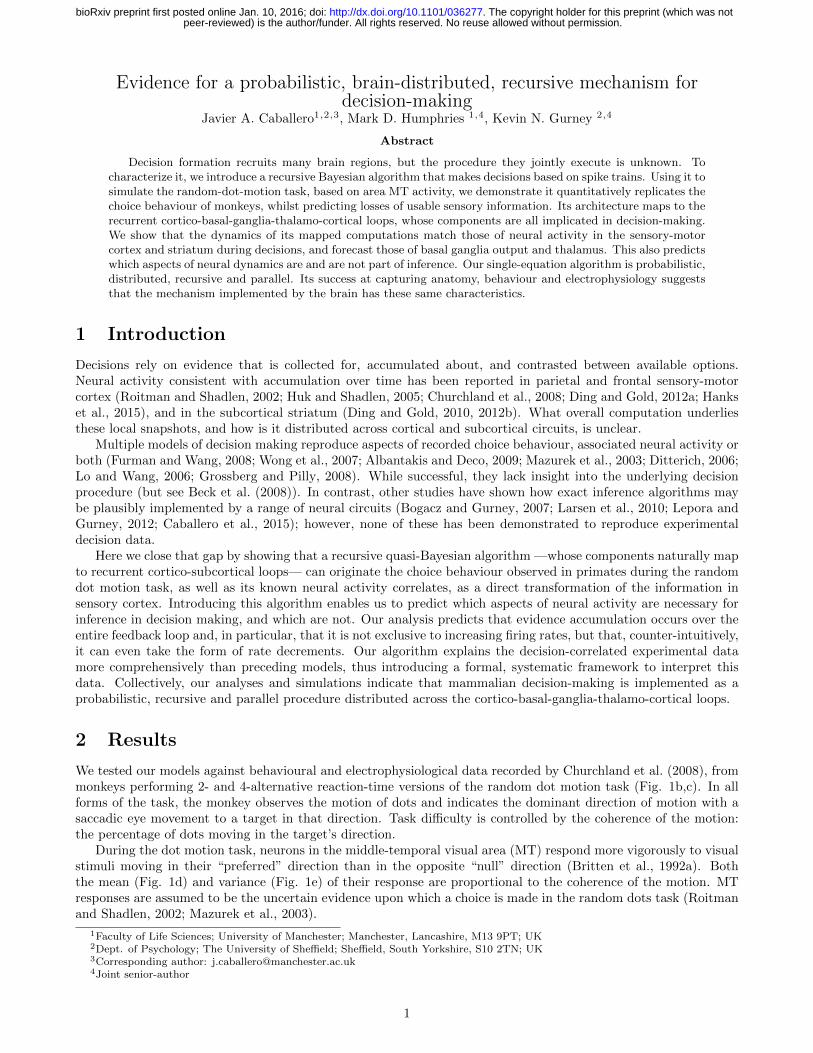
The (r)MSPRT framework suggests that decision times depend on the discrimination information in the evidence.Discrimination information here is measured as the divergence between the ISI distributions of MT neurons for dotsmoving in their preferred and null directions. Intuitively, the larger this divergence, the easier and hence faster thedecision. We can estimate how much discrimination information monkeys used by asking how much the (r)MSPRTwould require to obtain the same reaction times on correct trials as the monkeys, per condition. We thus find thatmonkeys tended to use less discrimination information than that in ISI distributions in their MT when making thedecision (Fig. 3b). In contrast, the (r)MSPRT uses the full discrimination information available. This implies thatthe decision-making mechanism in monkeys lost large proportions of MT discrimination information (Fig. 3c). Sincethese (r)MSPRT decision times are upper bounds, this in turn means that this loss of discrimination informationis the minimum.

2.3 (r)MSPRT with depleted information reproduces monkey performance

To verify if this information loss alone could account for the monkeys’ deviation from the (r)MSPRT upper bounds,we depleted the discrimination information of its input distributions to exactly match the estimated monkey lossin Fig. 3c per condition. We did so only by modifying the mean and standard deviation of the null direction ISIdistribution, to make it more similar to the preferred distribution (exemplified in Fig. 3d).

Using these information-depleted statistics, the mean reaction times predicted by the (r)MSPRT in correct trialsclosely match those of monkeys (Fig. 4a). Strikingly, although this information-depletion procedure is based onlyon data from correct trials, the (r)MSPRT now also matches closely the mean reaction times of monkeys from errortrials (Fig. 4b). Moreover, for both correct and error trials the (r)MSPRT accurately captures the relative scalingof mean reaction time by the number of alternatives (Fig. 4a,b).

The reaction time distributions of the model closely resemble those of monkeys in that they are positively skewedand exhibit shorter right tails for higher coherence levels (Fig. 4c-f). These qualitative features are captured acrossboth correct and error trials, and 2 and 4-alternative tasks. Together, these results support the hypothesis that theprimate brain approximates an algorithm similar to the rMSPRT.

4


http://dx.doi.org/10.1101/036277

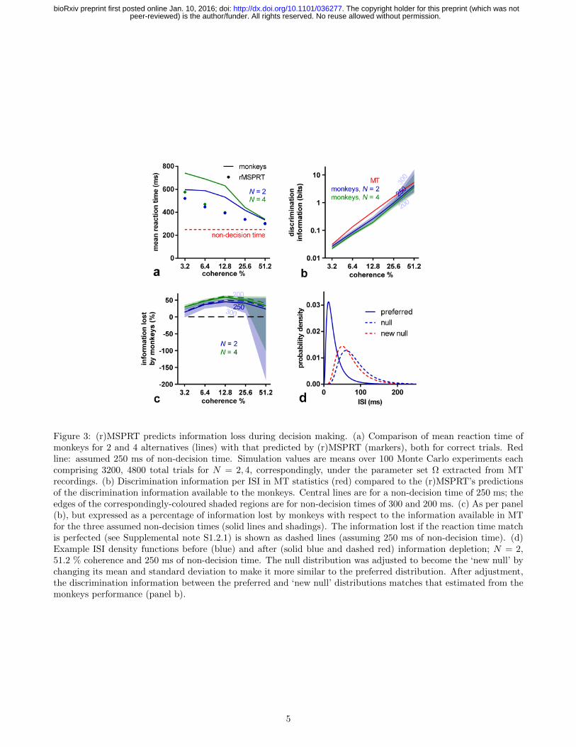
Figure 3: (r)MSPRT predicts information loss during decision making. (a) Comparison of mean reaction time ofmonkeys for 2 and 4 alternatives (lines) with that predicted by (r)MSPRT (markers), both for correct trials. Redline: assumed 250 ms of non-decision time. Simulation values are means over 100 Monte Carlo experiments eachcomprising 3200, 4800 total trials for N = 2, 4, correspondingly, under the parameter set Ω extracted from MTrecordings. (b) Discrimination information per ISI in MT statistics (red) compared to the (r)MSPRT’s predictionsof the discrimination information available to the monkeys. Central lines are for a non-decision time of 250 ms; theedges of the correspondingly-coloured shaded regions are for non-decision times of 300 and 200 ms. (c) As per panel(b), but expressed as a percentage of information lost by monkeys with respect to the information available in MTfor the three assumed non-decision times (solid lines and shadings). The information lost if the reaction time matchis perfected (see Supplemental note S1.2.1) is shown as dashed lines (assuming 250 ms of non-decision time). (d)Example ISI density functions before (blue) and after (solid blue and dashed red) information depletion; N = 2,51.2 % coherence and 250 ms of non-decision time. The null distribution was adjusted to become the ‘new null’ bychanging its mean and standard deviation to make it more similar to the preferred distribution. After adjustment,the discrimination information between the preferred and ‘new null’ distributions matches that estimated from themonkeys performance (panel b).

5


http://dx.doi.org/10.1101/036277

Figure 4: Monkey reaction times are consistent with (r)MSPRT using depleted discrimination information. (a,b) Mean reaction time of monkeys (lines) with 99 % Chebyshev confidence intervals (shading) and (r)MSPRTpredictions for correct (a; Eq. 1) and error trials (b; Eq. 2) when using information-depleted statistics (MTparameter set Ωd). (r)MSPRT results are means of 100 simulations with 3200, 4800 total trials each for N = 2, 4,respectively. Confidence intervals become larger in error trials because monkeys made fewer mistakes for highercoherence levels. (c-f) ‘Violin’ plots of reaction time distributions (vertically plotted histograms reflected aboutthe y-axis) from monkeys (red; 766–785, 1170–1217 trials for N = 2, 4, respectively) and (r)MSPRT when usinginformation-depleted statistics (blue; single example Monte Carlo simulation with 800, 1200 total trials forN = 2, 4).

6


http://dx.doi.org/10.1101/036277

2.4 rMSPRT maps onto cortico-subcortical circuitry

Beyond matching behaviour, we then asked whether the rMSPRT could account for the simultaneously recordedneural dynamics during decision making. To do so, we first must map its components to a neural circuit. Being ableto handle arbitrary signal delays means the rMSPRT could in principle map to a range of feedback neural circuits.Because cortex (Roitman and Shadlen, 2002; Huk and Shadlen, 2005; Churchland et al., 2008; Ding and Gold,2012a; Hanks et al., 2015), basal ganglia (Redgrave et al., 1999; Ding and Gold, 2010) and thalamus (Watanabeand Funahashi, 2004) have been implicated in decision-making, we sought a mapping that could account for theircollective involvement.

In the visuo-motor system, MT projects to the lateral intra-parietal area (LIP) and frontal eye fields (FEF)—the ‘sensory-motor cortex’. The basal ganglia receives topographically organized afferent projections (Heimeret al., 1995) from virtually the whole cortex, including LIP and FEF (Petras, 1971; Saint-Cyr et al., 1990; Hamaniet al., 2004). In turn, the basal ganglia provide indirect feedback to the cortex through thalamus (Alexander et al.,1986; Middleton and Strick, 2000). This arrangement motivated the feedback embodied in rMSPRT.

Multiple parallel recurrent loops connecting cortex, basal ganglia and thalamus can be traced anatomically(Alexander et al., 1986; Middleton and Strick, 2000). Each loop in turn can be sub-divided into topographicallyorganised parallel loops (Alexander and Crutcher, 1990; Middleton and Strick, 2000). Based on this, we conjecturethe organization of these circuits into N functional loops, for decision formation, to simultaneously evaluate thepossible hypotheses.

Our mapping of computations within the rMSPRT to the cortico-basal-ganglia-thalamo-cortical loop is shownin Fig. 5. Its key ideas are, first, that areas like LIP or FEF in the cortex evaluate the plausibility of all availablealternatives in parallel, based on the evidence produced by MT, and join this to any initial bias. Second, thatas these signals traverse the basal ganglia, they compete, resulting in a decision variable per alternative. Third,that the basal ganglia output nuclei uses these to assess whether to make a final choice and what alternative topick. Fourth, that decision variables are returned to LIP or FEF via thalamus, to become a fresh bias carryingall conclusions on the decision so far. The rMSPRT thus predicts that evidence accumulation happens in theoverall, large-scale loop, rather than in a single site. Lastly, our mapping of the rMSPRT provides an account forthe spatially diffuse cortico-thalamic projection (McFarland and Haber, 2002); it predicts the projection conveysa hypothesis-independent signal that does not affect the inference carried out by the loop, but may produce theincreasing offset required to facilitate the cortical re-use of inhibitory fed-back decision information from the basalganglia (see Supplemental note S1.2.2).

2.5 Electrophysiological comparison

With the mapping above, we can compare the proposed rMSPRT computations to recorded activity during decision-making in area LIP and striatum. We first consider the dynamics around decision initiation. During the dot motiontask, the mean firing rate of LIP neurons deviates from baseline into a stereotypical dip soon after stimulus onset,possibly indicating the reset of a neural integrator (Roitman and Shadlen, 2002; Furman and Wang, 2008). LIPresponses become choice- and coherence-modulated after the dip (Roitman and Shadlen, 2002). We thereforereasoned that LIP neurons engage in decision formation from the bottom of the dip and model their mean firingrate from then on. After this, mean firing rates “ramp-up” for ∼ 40 ms, then “fork”: they continue ramping-upif dots moved towards the response (or movement) field of the neuron (inRF trials; Fig. 6a, solid lines) or droptheir slope if the dots were moving away from its response field (outRF trials; dashed lines) (Roitman and Shadlen,2002; Churchland et al., 2008). The magnitude of LIP firing rate is also proportional to the number of availablealternatives (Fig. 6a,b) (Churchland et al., 2008).

The model LIP in rMSPRT (sensory-motor cortex) captures each of these properties: activity ramps fromthe start of the accumulation, forks between putative in- and out-RF responses, and scales with the number ofalternatives (Fig. 6c). Under this model, inRF responses in LIP occur when the likelihood function representedby neurons was best matched by the uncertain MT evidence; correspondingly, outRF responses occur when thelikelihood function was not well matched by the evidence.

The rMSPRT provides a mechanistic explanation for the ramp-and-fork pattern. Initial accumulation (steps0–2) occurs before the feedback has arrived at the model sensory-motor cortex, resulting in a ramp. The forking (atstep 3) is the point at which the posteriors from the output of the model basal ganglia first arrive at sensory-motorcortex to be re-used as priors. By contrast, non-recursive MSPRT (without feedback of posteriors) predicts well-separated neural signals throughout (Fig. 6e). Consequently, the rMSPRT suggests that the fork represents thetime at which updated signals representing the competition between alternatives —here posterior probabilities—are made available to the sensory-motor cortex.

7


http://dx.doi.org/10.1101/036277

Figure 5: Mapping of rMSPRT computations to the cortico-basal-ganglia-thalamo-cortical loops. (a) Mapping ofthe negative logarithm of rMSPRT components from Fig. 2. Sensory cortex (e.g. MT) produces fresh evidencefor the decision, delivered to sensory-motor cortex in C parallel channels (e.g. MT spike trains). Sensory-motorcortex (e.g. LIP or FEF) computes in parallel the simplified log-likelihoods of all hypotheses given this evidence andadds log-priors —or fed-back log-posteriors after the delay ∆ has elapsed. It also adds a hypothesis-independentbaseline comprising a simulated constant background activity (e.g. from LIP before stimulus onset) and a time-increasing term from the interaction with the thalamus. The basal ganglia bring the computations of all hypothesestogether into new negative log-posteriors that are then tested against a threshold. Negative log-posteriors will tendto decrease for the best-supported hypothesis and increase otherwise. This is consistent with the idea that basalganglia output selectively removes inhibition from a chosen motor program while increasing inhibition of competingprograms (Basso and Wurtz, 2002; Humphries et al., 2006; Bogacz and Gurney, 2007; Redgrave et al., 1999).Further details of this computation are in Supplemental Fig. S1. Finally, the thalamus conveys the updated log-posterior from basal ganglia output to be used as a log-prior by sensory-motor cortex. Thalamus’ baseline is givenby its diffuse feedback from sensory-motor cortex. (b) Corresponding formal mapping of rMSPRT’s computationalcomponents, showing how Eq. 13 decomposes. All computations are delayed with respect to the basal ganglia viathe integer latencies δpq, from p to q; where p, q ∈ y, b, u, y stands for the sensory-motor cortex, b for the basalganglia and u for the thalamus. ∆ = δyb + δbu + δuy with the requirement ∆ ≥ 1.

8


http://dx.doi.org/10.1101/036277

The rMSPRT further predicts that the scaling of activity in sensory-motor cortex by the number of alternativesis due to cortico-subcortical loops becoming organized as N parallel functional circuits, one per hypothesis. Thiswould determine the baseline output of the basal ganglia. Until task related signals reach the model basal ganglia,their output codes the initial priors for the set of N hypotheses. Their output is then an increasing function of thenumber of alternatives (Fig. 6f). This increased inhibition of thalamus in turn reduces baseline cortical activityas a function of N . The direct proportionality of basal ganglia output firing rate to N recorded in the substantianigra pars reticulata (SNr) of macaques during a fixed-duration choice task (Basso and Wurtz, 2002) lends supportto this hypothesis.

The rMSPRT also captures key features of dynamics at decision termination. For inRF trials, the mean firingrate of LIP neurons peaks at or very close to the time of saccade onset (Fig. 6b). By contrast, for outRF trialsmean rates appear to fall just before saccade onset. The rMSPRT can capture both these features (Fig. 6d) whenwe allow the model to continue updating after the decision rule (Eq. 14) is met. The decision rule is implementedat the output of the basal ganglia and the model sensory-motor cortex peaks just before the final posteriors havereached the cortex. The rMSPRT thus predicts that the activity in LIP lags the actual decision.

This prediction may explain an apparent paradox of LIP activity. The peri-saccadic population firing rate peakin LIP during inRF trials (Fig. 6b) is commonly assumed to indicate the crossing of a threshold and thus decisiontermination. Visuo-motor decisions must be terminated well before saccade to allow for the delay in the execution ofthe motor command, conventionally assumed in the range of 80–100 ms in macaques (Mazurek et al., 2003; Resulajet al., 2009). It follows that LIP peaks too close to saccade onset (∼ 15 ms before) for this peak to be causal. TherMSPRT suggests that the inRF LIP peak is not indicating decision termination, but is instead a delayed read-outof termination in an upstream location.

LIP firing rates are also modulated by dot-motion coherence (Fig. 7a,b,i,j). Following stimulus onset, theresponse of LIP neurons tends to fork more widely for higher coherence levels (Fig. 7a,i) (Roitman and Shadlen,2002; Churchland et al., 2008). The increase in activity before a saccade during inRF trials is steeper for highercoherence levels, reflecting the shorter average reaction times (Fig. 7b,j) (Roitman and Shadlen, 2002; Churchlandet al., 2008). The rMSPRT shows coherence modulation of both the forking pattern (Fig. 7c,k) and slope of activityincrease (Fig. 7d,l). rMSPRT also predicts that the apparent convergence of LIP activity to a common level ininRF trials is not required for inference and so may arise due to additional neural constraints. We take up thispoint in the Discussion.

Similar modulation of population firing rates during the dot motion task has been observed in the striatum(Ding and Gold, 2010). Naturally, the striatum in rMSPRT, which relays cortical input (Supplemental Fig. S1),captures this modulation (Supplemental Fig. S2).

2.6 Electrophysiological predictions

Our proposed mapping of the rMSPRT’s components (Fig. 5) makes testable qualitative predictions for the meanresponses in basal ganglia and thalamus during the dot motion task. For the basal ganglia output, likely from theoculomotor regions of the SNr, rMSPRT (like MSPRT) predicts a drop in the activity of output neurons in inRFtrials and an increase in outRF ones. It also predicts that these changes are more pronounced for higher coherencelevels (Fig. 7e,f,m,n). These predictions are consistent with recordings from macaque SNr neurons showing thatthey suppress their inhibitory activity during visually or memory guided saccade tasks, in putative support ofsaccades towards a preferred region of the visual field (Handel and Glimcher, 1999; Basso and Wurtz, 2002), andenhance it otherwise (Handel and Glimcher, 1999).

For visuo-motor thalamus, rMSPRT predicts that the time course of the mean firing rate will exhibit a ramp-and-fork pattern similar to that in LIP (Fig. 7g,h,o,p). The separation of in- and out-RF activity is consistent withthe results of Watanabe and Funahashi (2004) who found that, during a memory-guided saccade task, neurons inthe macaque medio-dorsal nucleus of the thalamus (interconnected with LIP and FEF), responded more vigorouslywhen the target was flashed within their response field than when it was flashed in the opposite location.

2.7 Predictions for neural activity features not crucial for inference

Understanding how a neural system implements an algorithm is complicated by the need to identify which featuresare core to executing the algorithm, and which are imposed by the constraints of implementing computations usingneural elements —for example, that neurons cannot have negative firing rates, so cannot straightforwardly representnegative numbers. The three free parameters in the rMSPRT allow us to propose which functional and anatomicalproperties of the cortico-basal-ganglia-thalamo-cortical loop are workarounds within these constraints, but do notaffect inference.

9


http://dx.doi.org/10.1101/036277

Figure 6: Example LIP firing rate patterns and predictions of rMSPRT and MSPRT at 25.6 % coherence. (a, b)Mean population firing rate of LIP neurons during correct trials on the reaction-time version of the dot motiontask. By convention, inRF trials are those when recorded neurons had the motion-cued target inside their responsefield (solid lines); outRF trials are those when recorded neurons had the motion-cued target outside their responsefield (dashed lines). (a) Aligned at stimulus onset, starting at the stereotypical dip, illustrating the “ramp-and-fork” pattern between average inRF and outRF responses. (b) Aligned at saccade onset (vertical dashed line). (c,d) Mean time course of the model sensory-motor cortex in rMSPRT aligned at decision initiation (c; t = 1) andtermination (d; Term; dotted line), for correct trials. Initiation and termination are with respect to the time ofbasal ganglia output. Note the suggested saccade time “Sac?”, close to the peak of inRF computations. Simulationsare a single Monte Carlo experiment with 800, 1200 total trials for N = 2, 4, respectively, using parameter set Ωd.We include an additional step at −1 determined only by initial priors and baseline, where no inference is carried out(yi (t+ δyb) = 0 for all i). Conventions as in (a). (e) Same as in (c), but for the standard, non-recursive MSPRT(defined as Eq. 14 using only the first case of Eqs. 12 and 13). (f) Baseline output of the model basal gangliaincreases as a function of the number of alternatives, thus increasing the initial inhibition of thalamus and cortex.For uniform priors, the rMSPRT predicts this function is: − logP (Hi) = − log (1/N). Coloured dots indicateN = 2 (blue) and N = 4 (green).

10


http://dx.doi.org/10.1101/036277

200 400 6000

20

40

60

80

time (ms)

LIP

(Hz)

Stim

a

-600 -400 -200 Sac

3.26.4

12.825.651.2

b

200 400 6000

20

40

60

80

time (ms)Stim

i

-600 -400 -200 Sac

j

15

20

25

30

35

40

sen

so

ry-m

oto

rco

rtex

c d

15

20

25

30

35

40k l

0

2

4

6

8

basalg

an

glia

ou

tpu

t

e f

0

2

4

6

8m n

-5 0 50

5

10

time step

thala

mu

s

Init

g

-6 -4 -2 2Term

h

-5 0 50

2

4

6

8

10

time stepInit

o

-8 -6 -4 -2 2Term

p

N = 2 N = 4

mo

nkeys

rMS

PR

T

Figure 7: Modulation of activity by coherence throughout the cortico-basal-ganglia-thalamo-cortical loop. (a-h)N = 2. (i-p) N = 4. Top row: mean firing rate in LIP over time, aligned to stimulus onset (Stim; a, i) or saccadeonset (Sac; b, j) (vertical dashed lines). (c-h, k-p) mean rMSPRT computations as mapped in Fig. 5, aligned atdecision initiation or termination (Init/Term; dotted lines); single Monte Carlo experiment with 800, 1200 totaltrials for N = 2, 4, respectively. (c, d, k, l) predicted time course of the model sensory-motor cortex (e.g. LIP). (e,f, m, n) predicted simultaneous course of mean firing rate in SNr. (g, h, o, p) predicted course in thalamic relaynuclei. Solid: inRF. Dashed: outRF. Coherence % as in legend. Unshaded regions indicate approximate periodswhere a mechanism of decision formation should aim to reproduce the recordings.

11


http://dx.doi.org/10.1101/036277

Figure 8: Effect of variations of free parameters on the time course of the model LIP in rMSPRT. Each solid anddashed set of lines is the mean of correct trials in a single Monte Carlo experiment, with 800 total trials, 25.6% coherence and N = 2. Computations aligned at decision initiation. Solid: inRF. Dashed: outRF. Blue: withparameters as tuned for this study. Green: increasing parameter value by 50 %, keeping other parameters as tuned.Red: decreasing it by 50 %, keeping others as tuned. Black: removing the effect of the tested parameter (l = 0,wyu = 0, n = 1), keeping others as tuned. (a) Varying the baseline, l. (b) Varying the cortico-thalamic weight,wyu. (c) Varying the data scaling factor n.

One free parameter enforces the baseline activity that LIP neurons maintain before and during the initialstimulus presentation (Fig. 7a,i). Varying this parameter, l, scales the overall activity of LIP, but does not changethe inference performed (Fig. 8a). Consequently, this suggests that the baseline activity of LIP depends on N butdoes not otherwise affect the inference algorithm implemented by the brain.

The second free parameter, wyt, sets the strength of the spatially diffuse projection from cortex to thalamus.Varying this weight changes the forking between inRF and outRF computations but does not affect inference(Fig. 8b). The third free parameter, n, sets the overall, hypothesis-independent temporal scale at which sampledinput ISIs are processed; changing n varies the slope of sensory-motor computations, even allowing all-decreasingpredicted mean firing rates (Fig. 8c). By definition, the log-likelihood of a sequence tends to be negative and decreasemonotonically as the sequence lengthens. Introducing n is required to get positive simplified log-likelihoods, capableof matching the neural activity dynamics, without affecting inference. Hence, n may capture a workaround of thedecision-making circuitry to represent these whilst avoiding signal ‘underflow’, by means of scaling the input data.

Traditionally, evidence accumulation is exclusively associated with increasing firing rates during decision, andprevious studies have questioned whether the often-observed decision-correlated yet non-increasing firing rates (e.g.in outRF conditions in Fig. 7a,i and Roitman and Shadlen (2002); Churchland et al. (2008); Huk and Shadlen(2005); Hernandez et al. (2002); Hanks et al. (2015); Kira et al. (2015)) are consistent with accumulation (Parket al., 2014). The diversity of patterns predicted by rMSPRT in sensory-motor cortex (Fig. 8) solves this bydemonstrating that both increasing and non-increasing activity patterns can house evidence accumulation.

12


http://dx.doi.org/10.1101/036277

3 Discussion

We sought to characterize the mechanism that underlies decisions by using the knowable function of a normativealgorithm —the rMSPRT— as a systematic framework. With the currently available range of experimental studiesgiving us local snapshots of cortical and sub-cortical activity during decision-making tasks, the rMSPRT showsus how, where, and when these snapshots fit into a complete inference procedure. While it is not plausible thatthe brain implements exactly a specific algorithm, our results suggest that the essential structure of its underlyingdecision mechanism includes the following. First, that the mechanism is probabilistic in nature —the brain utilizesthe uncertainty in neural signals, rather than suffering from it. Second, that the mechanism works entirely ‘on-line’,continuously updating representations of hypotheses that can be queried at any time to make a decision. Third,that this processing is distributed, recursive and parallel, producing a decision variable for each available hypothesis.And fourth, that this recursion allows the mechanism to adapt to the observed statistics of the environment, as itcan re-use updated probabilities about hypotheses as priors for upcoming decisions.

We have pushed the analogy between a single-equation statistical test and the neural decision-making algorithm along way before it broke down. We find it remarkable that, starting from data-constrained spike-trains, a monolithicstatistical test in the form of the rMSPRT can simultaneously account for much of the anatomy, behaviour andelectrophysiology of decision-making.

3.1 Why implement a recursive algorithm in the brain?

Prior work proposed that the cortex and basal ganglia alone could implement the non-recurrent MSPRT (Bogacz andGurney, 2007; Lepora and Gurney, 2012). However, the looped cortico-basal-ganglia-thalamo-cortical architectureimplies a recursive computation. This raises the question of why such a complex, distributed feedback architectureexists.

First, recursion makes trial-to-trial adaptation of decisions possible. Priors determined by previous stimulation(fed-back posteriors), can bias upcoming similar decisions towards the expected best choice, even before any newevidence is collected. This can shorten reaction times in future familiar settings without compromising accuracy.

Second, recursion provides a robust memory. A posterior fed-back as a prior is a sufficient statistic of all pastevidence observations. That is, it has taken ‘on-board’ all sensory information since the decision onset. In rMSPRT,accumulation happens over the whole cortico-subcortical loop, so the sensory-motor cortex only need keep track ofobservations in a moving time window of maximum width ∆ —the delay around the loop– rather than keeping trackof the entire sequence of observations. For a physical substrate subject to dynamics and leakage, like a neuron inLIP or FEF, this has obvious advantages: it would reduce the demand for keeping a perfect record (e.g. likelihood)of all evidence, from the usual hundreds of milliseconds in decision times to the ∼ 30 ms of latency around thecortico-basal-ganglia-thalamo-cortical loop (adding up estimates from Nambu et al. (1988); Hikosaka et al. (1993);Gerfen and Wilson (1996)).

3.2 Lost information and perfect integration

The rMSPRT predicts that monkeys do not make full use of the discrimination information available in MT (Fig.3b). Here rMSPRT needs only C = N MT spike-trains to outperform monkeys: as this is the upper bound ofrMSPRT mean decision time, this implies the monkey’s predicted loss (Fig. 3c) is a minimum.

This gap arises because rMSPRT is a generative model of the task, which assumes initial knowledge of coherence,which in turn determines appropriate likelihoods for the task at hand. Any deviation from this ideal will tend todegrade performance (Beck et al., 2012), whether it comes from one or more of the inherent leakiness of neurons,correlations, or the coherence to likelihood mapping (Caballero et al., 2015). LIP neurons change their codingduring learning of the dot motion task and MT neurons do not (Law and Gold, 2008), implying that learning thetask requires mapping of MT to LIP populations by synaptic plasticity (Law and Gold, 2009). Consequently, evenif the MT representation is perfect, the learnt mapping only need satisfice the task requirements, not optimallyperform.

Excellent matches to performance in both correct and error trials were obtained solely by accounting for lostinformation in the evidence streams. No noise was added within the rMSPRT itself. Prior experimental workreported perfect, noiseless integration by both rat and human subjects performing an auditory task, attributingall effects of noise on task performance to the variability in the sensory input (Brunton et al., 2013). Our resultsextend this observation to primate performance on the dot motion task, and further support the idea that theneural decision-making mechanism can perform perfect integration of uncertain evidence.

13


http://dx.doi.org/10.1101/036277

3.3 Neural response patterns during decision formation

Neurons in LIP, FEF (Ding and Gold, 2012a) and striatum (Ding and Gold, 2010) exhibit a ramp-and-fork patternduring the dot motion task. Analogous choice-modulated patterns have been recorded in the medial premotor cortexof the macaque during a vibro-tactile discrimination task (Hernandez et al., 2002) and in the posterior parietal cortexand frontal orienting fields of the rat during an auditory discrimination task (Hanks et al., 2015). The rMSPRTindicates that such slow dynamics emerge from decision circuits with a delayed, inhibitory drive within a loopedarchitecture. Together, this suggests that decision formation in mammals may approximate a common recursivecomputation.

A random dot stimulus pulse delivered earlier in a trial has a bigger impact on LIP firing rate than a later one(Huk and Shadlen, 2005). This highlights the importance of capturing the initial, early-evidence ramping-up beforethe forking. However, multiple models omit it, focusing only on the forking (e.g. Mazurek et al. (2003); Ditterich(2006); Beck et al. (2008)). Other, heuristic models account for LIP activity from the onset of the choice targets,through dots stimulation and up until saccade onset (e.g. Wong et al. (2007); Grossberg and Pilly (2008); Furmanand Wang (2008); Albantakis and Deco (2009)). Nevertheless, their predicted firing rates rely on two fitted heuristicsignals that shape both the dip and the ramp-and-fork pattern. In contrast, the ramp-and-fork dynamics emergenaturally from the delayed inhibitory feedback in rMSPRT during decision formation (see Supplemental note S1.2.3for more details on the relation of the rMSPRT to prior models of decision-making).

rMSPRT replicates the ramp-and-fork pattern for individual coherence levels and given N (Fig. 6). However,comparing its predictions across N (Fig. 6d) or over coherence levels (Fig. 7d,l) reveals that the model sensory-motor cortex does not converge to a common value around decision termination in inRF trials, as the LIP does(Fig. 6b, Fig. 7b,j and Churchland et al. (2008)). Here we have reached the limits where the direct comparison ofthe single-equation statistical test to neural signals breaks down. Our mapping of rMSPRT onto the cortico-basal-ganglia-thalamo-cortical circuitry suggests the core underlying computation contributed per site during decisionformation (Fig. 5); that is, what is required for inference, such as the negative log-posterior probability at the basalganglia. Even if these suggestions are accurate, we would still expect other factors to influence the dynamics ofrecorded neural signals. These regions after all engage in multiple other computations, some of which are likelyorthogonal to decision formation.

One possibility is that the convergence of LIP activity to a common value just prior to saccade onset mayresult from monotonic transformations of these core computations. For instance, the successful fitting of previouscomputational models to neural data has been critically dependent on the addition of heuristic signals (Wong et al.,2007; Grossberg and Pilly, 2008; Furman and Wang, 2008; Albantakis and Deco, 2009). The incorporation ofsimilar heuristic signals may also convert the present qualitative resemblance of the recordings, by rMSPRT, to aquantitative reproduction. This is, however, beyond the scope of this study, whose aim is to test how closely anormative mechanism can explain behaviour and electrophysiology during decisions.

3.4 Emergent predictions

Inputs to the rMSPRT were determined solely from MT responses during the dot-motion task, and it has onlythree free parameters, none of which affect inference. It is thus surprising that it renders emergent predictionsthat are consistent with experimental data. First, our information-depletion procedure used exclusively statisticsfrom correct trials. Yet, after depletion, rMSPRT matches monkey behaviour in correct and error trials (Fig. 4),suggesting a mechanistic connection between them in the monkey that is naturally captured by rMSPRT. Second,the values of the three free parameters were chosen solely so that the model LIP activity resembled the ramp-and-fork pattern observed in our LIP data-set (Fig. 6a,c). As demonstrated in Fig. 8, the ramp-and-fork pattern isa particular case of two-stage patterns that are an intrinsic property of the rMSPRT, guaranteed by the feedbackof the posterior after the delay ∆ has elapsed (Eq. 9). Nonetheless, the model also matches LIP dynamics whenaligned at decision termination (panels b and d). Third, the predictions of the time course of the firing rate in SNrand thalamic nuclei naturally emerge from the functional mapping of the algorithm onto the cortico-basal-ganglia-thalamo-cortical circuitry. These are already congruent with existing electrophysiological data; however, their fullverification awaits recordings from these sites during the dot motion task. These and other emergent predictions arean encouraging indicator of the explanatory power of a systematic framework for understanding decision formation,embodied by the rMSPRT.

14


http://dx.doi.org/10.1101/036277

4 Experimental Procedures

4.1 Experimental paradigms

Behavioural and neural data was collected in two previous studies (Britten et al., 1992a; Churchland et al., 2008),during two versions of the random dots task (Fig. 1a-c). Detailed experimental protocols can be found in suchstudies. Below we briefly summarize them.

4.1.1 Fixed duration

Three rhesus macaques (Macaca mulatta) were trained to initially fixate their gaze on a visual fixation point (crossin Fig. 1a). A random dot kinematogram appeared covering the response field of the MT neuron being recorded(grey patch); task difficulty was controlled per trial by the proportion of dots (coherence %) that moved in one oftwo directions: that to which the MT neuron was tuned to —its preferred motion direction— or its opposite —nullmotion direction. After 2 s the fixation point and kinematogram vanished and two targets appeared in the possiblemotion directions. Monkeys received a liquid reward if they then saccaded to the target towards which the dots inthe stimulus were predominantly moving (Britten et al., 1992a).

4.1.2 Reaction time

Two macaques learned to fixate their gaze on a central fixation point (Fig. 1b,c). Two (Fig. 1b) or four (Fig.1c) eccentric targets appeared, signalling the number of alternatives in the trial, N ; one such target fell within theresponse (movement) field of the recorded LIP neuron (grey patch). This is the region of the visual field towardswhich the neuron would best support a saccade. Later a random dot kinematogram appeared where a controlledproportion of dots moved towards one of the targets. The monkeys received a liquid reward for saccading to theindicated target when ready (Churchland et al., 2008).

4.2 Data analysis

For comparability across databases, we only analysed data from trials with coherence levels of 3.2, 6.4, 12.8, 25.6,and 51.2 %, unless otherwise stated. We used data from all neurons recorded in such trials. This is, between 189and 213 visual-motion-sensitive MT neurons (see table S1; data from Britten et al. (1992a,b)) and 19 LIP neuronswhose activity was previously determined to be choice- and coherence-modulated (data from Churchland et al.(2008)). The behavioural data analysed was that associated to LIP recordings. For MT, we analysed the neuralactivity between the onset and the vanishing of the stimulus. For LIP we focused on the period between 100 msbefore stimulus onset and 100 ms after saccade onset.

To estimate moving statistics of neural activity we first computed the spike count over a 20 ms window slidingevery 1 ms, per trial. The moving mean firing rate per neuron per condition was then the mean spike count over thevalid bins of all trials divided by the width of this window; the standard deviation was estimated analogously. LIPrecordings were either aligned at the onset of the stimulus or of the saccade; after or before these (respectively),data was only valid for a period equal to the reaction time per trial. The population moving mean firing rate is themean of single-neuron moving means over valid bins; analogously, the population moving variance of the firing rateis the mean of single neuron moving variances. For clarity, population statistics were then smoothed by convolvingthem with a Gaussian kernel with a 10 ms standard deviation. The resulting smoothed population moving statisticsfor MT are in Fig. 1d,e. In Figs. 6a,b and 7a,b,i,j smoothed mean LIP firing rates are plotted only up to themedian reaction time plus 80 ms, per condition.

Analogous procedures were used to compute the moving mean of rMSPRT computations, per time step. Theseare shown up to the median of termination observations plus 3 time steps in Figs. 6c-e and 7c-h,k-p.

4.3 Spikes and continuous time out of discrete time

We have defined rMSPRT to operate over a discrete time line; however, the brain operates over continuous time.Caballero et al. (2015) introduced a continuous-time generalization of MSPRT that uses spike-trains as inputs fordecision. Thence, the length of ISIs was random and their sum up until decision is, by definition, a continuouslydistributed time. With all other assumptions equal, Caballero et al. (2015) demonstrated that, as an average, thetraditional discrete-time MSPRT requires the same number of observations to decision, as the ISIs required by themore general spike-based MSPRT. This means that the number of observations to decision, T , in (r)MSPRT has

15


http://dx.doi.org/10.1101/036277

an interpretation as continuously-distributed time. So, the expected decision sample size for correct choices, 〈T 〉c,required by the simpler discrete-time (r)MSPRT, can be interpreted as the mean decision time

τc = (〈T 〉c + 0.5)µ∗n (1)

predicted by the more general continuous-time, spike-based MSPRT, where µ∗n is the mean ISI produced bya MT neuron whose preferred motion direction was matched by the stimulus and was thus firing the fastest onaverage. When the mean firing rate to a preferred characteristic of the stimulus is larger than that to a non-preferredone (µ∗ < µ0) —as in MT (Britten et al., 1992a), middle-lateral and anterolateral auditory cortex (Tsunada et al.,2016)— the hypothesis selected in error trials is that misinformed by channels with mean µ0n which intuitivelyhappened to fire faster than those whose mean was actually µ∗n. Hence, the mean decision time predicted byrMSPRT in error trials would be:

τe = (〈T 〉e + 0.5)µ0n, (2)

where 〈T 〉e is the mean decision sample size for error trials. An instance of rMSPRT capable of making choicesupon sequences of spike-trains is straightforward from the formal framework above and that introduced by Caballeroet al. (2015); nevertheless, for simplicity here we choose to work with the discrete-time rMSPRT. After all, thanksto Eqs. 1 and 2 we can still interpret its behaviour-relevant predictions in terms of continuous time. We use theseto compute the decision times that originate the reaction times in Figs. 3 and 4.

4.4 Estimation of lost information

We outline here how we use the monkeys’ reaction times on correct trials and the properties of the rMSPRT, toestimate the amount of discrimination information lost by the animals. This is, the gap between all the informationavailable in the responses of MT neurons, as fully used by the rMSPRT in Fig. 3a, and the fraction of suchinformation actually used by monkeys.

The expected number of observations to reach a correct decision for (r)MSPRT, 〈T 〉c, depends on two quantities.First, the mean total discrimination information required for the decision, I (ε,N), that depends only on the errorrate ε, and N . Second, the ‘distance’ between distributions of ISIs from MT neurons facing preferred and nulldirections of motion (Caballero et al., 2015). This distance is the Kullback-Leibler divergence from f∗ to f0

D =

∫x

f∗ (x) log2

(f∗ (x)

f0 (x)

)dx

which measures the discrimination information available between the distributions. Using these two quantities,the decision time in the (r)MSPRT is (Caballero et al., 2015):

〈T 〉c ≥I (ε,N)

D, (3)

The product of our Monte Carlo estimate of 〈T 〉c in the rMSPRT (which originated Fig. 3a) and D from the

MT ISI distributions (Fig. 1f), gives an estimate of the limit I (ε,N) in expression 3, denoted by I (ε,N).The ‘mean decision sample size’ of monkeys —hence the superscript m— within this framework corresponds

to ˆ〈T 〉m

c = (τmc /µ

∗n) − 0.5 (from Eq. 1). Here, τmc is the estimate of the mean decision time of monkeys for

correct choices, per condition; that is, the reaction time from Fig. 3a minus some constant non-decision time. Withˆ〈T 〉

m

c and I (ε,N), we can estimate the corresponding discrimination information available to the monkeys in this

framework as Dm = I (ε,N) / ˆ〈T 〉m

c (from expression 3).

Fig. 3b compares D (red line) to Dm (blue/green lines and shadings) for monkeys, using non-decision times ina plausible range of 200–300 ms. Fig. 3c shows the discrimination information lost by monkeys as the percentage

of D,[1−

(Dm/D

)]× 100 %.

4.5 Information depletion procedure

Expression 3 implies that the reaction times predicted by rMSPRT should match those of monkeys if we make thealgorithm lose as much information as the monkeys did. We did this by producing a new parameter set that bringsf0 closer to f∗ per condition, assuming 250 ms of non-decision time; critically, simulations like those in Fig. 4 willgive about the same rMSPRT reaction times regardless of the non-decision time chosen, as long as it is the sameassumed in the estimation of lost information and this information-depletion procedure.

16


http://dx.doi.org/10.1101/036277

An example of the results of information depletion in one condition is in Fig. 3d. We start with the originalparameter set extracted from MT recordings, Ω (‘preferred’ and ‘null’ densities in Fig. 3d), and keep µ∗ and σ∗fixed. Then, we iteratively reduce/increase the differences |µ0 − µ∗| and |σ0 − σ∗| by the same proportion, untilwe get new parameters µ0 and σ0 that, together with µ∗and σ∗, specify preferred (‘preferred’ in Fig. 3d) and null(‘new null’) density functions that bear the same discrimination information estimated for monkeys, Dm; hence,they exactly match the information loss in the solid lines in Fig. 3c. Intuitively, since the ‘new null’ distribution inFig. 3d is more similar to the ‘preferred’ one than the ‘null’, the Kullback-Leibler divergence between the first twois smaller than that between the latter two. The resulting parameter set is dubbed Ωd and reported in table S1.

4.6 Simulation procedures

For rMSPRT decisions to be comparable to those of monkeys, they must exhibit the same error rate, ε ∈ [0, 1]. Errorrates are taken to be an exponential function of coherence (%), s, fitted by non-linear least squares (R2 > 0.99)to the behavioural psychometric curves from the analysed LIP database, including 0 and 72.4 % coherence for thispurpose. This resulted in:

ε =

0.50 exp (−0.11s) , for N = 2

0.75 exp (−0.08s) , for N = 4(4)

Since monkeys are trained to be unbiased regarding choosing either target, initial priors for rMSPRT are set flat(P (Hi) = 1/N for all i) in every simulation. During each Monte Carlo experiment, rMSPRT made decisions witherror rates from Eq. 4. The value of the threshold, θ, was iteratively found to satisfy ε per condition (Caballeroet al., 2015); an example of the θs found is shown in Fig. S3a in the Supplement. Decisions were made overdata, xj (t) /n, randomly sampled from lognormal distributions specified for all channels by means and standarddeviations µ0 and σ0, respectively. The exception was a single channel where the sampled distribution was specifiedby µ∗ and σ∗. This models the fact that MT neurons respond more vigorously to visual motion in their preferreddirection compared to motion in a null direction, e.g. against the preferred. Effectively, this simulates macaque MTneural activity during the random dot motion task. The same parameters were used to specify likelihood functionsper experiment. All statistics were from either the Ω or Ωd parameter sets as noted per case. Note that the statisticsactually used in the simulations are those from MT in table S1, divided by the scaling factor n.

Author Contributions JAC deduced the rMSPRT, and performed all simulations and data analyses; all authorsdiscussed the results and wrote the article.

Acknowledgements We thank Anne Churchland, Roozbeh Kiani and Michael Shadlen for sharing their experi-mental data and the Humphries lab (Abhinav Singh, Mathew Evans and Silvia Maggi), Rafal Bogacz and LongDing for discussions. This work was supported by a National Council of Science and Technology (CONACyT)Fellowship (JAC) and a Medical Research Council Senior non-Clinical Fellowship (MDH).

References

Albantakis, L. and Deco, G. (2009). The encoding of alternatives in multiple-choice decision making. Proc NatlAcad Sci U S A, 106, 10308–10313.

Alexander, G. E. and Crutcher, M. D. (1990). Functional architecture of basal ganglia circuits: neural substratesof parallel processing. Trends Neurosci, 13, 266–271.

Alexander, G. E., DeLong, M. R., and Strick, P. L. (1986). Parallel organization of functionally segregated circuitslinking basal ganglia and cortex. Annu Rev Neurosci, 9, 357–381.

Basso, M. A. and Wurtz, R. H. (2002). Neuronal activity in substantia nigra pars reticulata during target selection.J Neurosc, 22, 1883–1894.

Baum, C. and Veeravalli, V. (1994). A sequential procedure for multihypothesis testing. IEEE T Inform Theory,40, 1994–2007.

Beck, J. M., Ma, W., Kiani, R., Hanks, T., Churchland, A. K., Roitman, J., Shadlen, M. N., Latham, P. E., andPouget, A. (2008). Probabilistic population codes for bayesian decision making. Neuron, 60, 1142–1152.

17


http://dx.doi.org/10.1101/036277

Beck, J. M., Ma, W. J., Pitkow, X., Latham, P. E., and Pouget, A. (2012). Not noisy, just wrong: the role ofsuboptimal inference in behavioral variability. Neuron, 74, 30–39.

Bogacz, R., Brown, E., Moehlis, J., Holmes, P., and Cohen, J. D. (2006). The physics of optimal decision making:a formal analysis of models of performance in two-alternative forced-choice tasks. Psychol Rev, 113, 700–765.

Bogacz, R. and Gurney, K. (2007). The basal ganglia and cortex implement optimal decision making betweenalternative actions. Neural Comput, 19, 442–477.

Bogacz, R. and Larsen, T. (2011). Integration of reinforcement learning and optimal decision-making theories ofthe basal ganglia. Neural Comput.

Britten, K. H., Shadlen, M. N., Newsome, W. T., and Movshon, J. A. (1992a). The analysis of visual motion: acomparison of neuronal and psychophysical performance. J Neurosci, 12, 4745–4765.

Britten, K. H., Shadlen, M. N., Newsome, W. T., and Movshon, J. A. (1992b). Responses of single neuronsin macaque MT/V5 as a function of motion coherence in stochastic dot stimuli, Neur Sig Arch, NSA2004.1.www.neuralsignal.org.

Brunton, B. W., Botvinick, M. M., and Brody, C. D. (2013). Rats and humans can optimally accumulate evidencefor decision-making. Science, 340, 95–98.

Caballero, J. A., Lepora, N. F., and Gurney, K. N. (2015). Probabilistic decision making with spikes: From ISIdistributions to behaviour via information gain. PLoS ONE, 10, e0124787.

Churchland, A. K., Kiani, R., and Shadlen, M. N. (2008). Decision-making with multiple alternatives. Nat Neurosci,11, 693–702.

Ding, L. and Gold, J. I. (2010). Caudate encodes multiple computations for perceptual decisions. J Neurosci, 30,15747–15759.

Ding, L. and Gold, J. I. (2012a). Neural correlates of perceptual decision making before, during, and after decisioncommitment in monkey frontal eye field. Cereb Cortex, 22, 1052–1067.

Ding, L. and Gold, J. I. (2012b). Separate, causal roles of the caudate in saccadic choice and execution in aperceptual decision task. Neuron, 75, 865–874.

Ding, L. and Gold, J. I. (2013). The basal ganglia’s contributions to perceptual decision making. Neuron, 79,640–649.

Ditterich, J. (2006). Stochastic models of decisions about motion direction: behavior and physiology. NeuralNetworks, 19, 981–1012.

Ditterich, J. (2010). A comparison between mechanisms of multi-alternative perceptual decision making: Ability toexplain human behavior, predictions for neurophysiology, and relationship with decision theory. Front Neurosci,4, 184.

Drugowitsch, J., Moreno-Bote, R., Churchland, A. K., Shadlen, M. N., and Pouget, A. (2012). The cost ofaccumulating evidence in perceptual decision making. J Neurosci, 32, 3612–3628.

Furman, M. and Wang, X.-J. (2008). Similarity effect and optimal control of multiple-choice decision making.Neuron, 60, 1153–1168.

Gerfen, C. R. and Wilson, C. J. (1996). Chapter II, the basal ganglia. In Integraded systems of the CNS, part IIICerebellum, basal ganglia, olfactory system, L. Swanson, A. Bjorklund, and T. Hokfelt, eds., vol. 12 of Handbookof Chemical Neuroanatomy. (Elsevier), pp. 371 – 468.

Grossberg, S. and Pilly, P. K. (2008). Temporal dynamics of decision-making during motion perception in the visualcortex. Vision Res, 48, 1345–1373.

Hamani, C., Saint-Cyr, J. A., Fraser, J., Kaplitt, M., and Lozano, A. M. (2004). The subthalamic nucleus in thecontext of movement disorders. Brain, 127, 4–20.

18


http://dx.doi.org/10.1101/036277

Handel, A. and Glimcher, P. W. (1999). Quantitative analysis of substantia nigra pars reticulata activity during avisually guided saccade task. J Neurophysiol, 82, 3458–3475.

Hanks, T. D., Kopec, C. D., Brunton, B. W., Duan, C. A., Erlich, J. C., and Brody, C. D. (2015). Distinctrelationships of parietal and prefrontal cortices to evidence accumulation. Nature, 520, 220–223.

Heimer, L., Zahm, D. S., and Alheid, G. F. (1995). Basal ganglia. In The Rat Nervous System, G. Paxinos, ed.(USA: Academic Press), 2nd edn., pp. 579–628.

Hernandez, A., Zainos, A., and Romo, R. (2002). Temporal evolution of a decision-making process in medialpremotor cortex. Neuron, 33, 959–972.

Hikosaka, O., Sakamoto, M., and Miyashita, N. (1993). Effects of caudate nucleus stimulation on substantia nigracell activity in monkey. Exp Brain Res, 95, 457–472.

Huk, A. C. and Shadlen, M. N. (2005). Neural activity in macaque parietal cortex reflects temporal integration ofvisual motion signals during perceptual decision making. J Neurosc, 25, 10420–10436.

Humphries, M. D., Stewart, R. D., and Gurney, K. N. (2006). A physiologically plausible model of action selectionand oscillatory activity in the basal ganglia. J Neurosci, 26, 12921–12942.

Kira, S., Yang, T., and Shadlen, M. N. (2015). A neural implementation of wald’s sequential probability ratio test.Neuron, 85, 861–873.

Larsen, T., Leslie, D. S., Collins, E. J., and Bogacz, R. (2010). Posterior weighted reinforcement learning with stateuncertainty. Neural Comput, 22, 1149–1179.

Law, C.-T. and Gold, J. I. (2008). Neural correlates of perceptual learning in a sensory-motor, but not a sensory,cortical area. Nat Neurosc, 11, 505–513.

Law, C.-T. and Gold, J. I. (2009). Reinforcement learning can account for associative and perceptual learning ona visual-decision task. Nat Neurosci, 12, 655–663.

Lepora, N. F. and Gurney, K. N. (2012). The basal ganglia optimize decision making over general perceptualhypotheses. Neural Comput, 24, 2924–2945.

Lo, C.-C. and Wang, X.-J. (2006). Cortico-basal ganglia circuit mechanism for a decision threshold in reaction timetasks. Nat Neurosci, 9, 956–963.

Mazurek, M. E., Roitman, J. D., Ditterich, J., and Shadlen, M. N. (2003). A role for neural integrators in perceptualdecision making. Cereb Cortex, 13, 1257–1269.

McFarland, N. R. and Haber, S. N. (2002). Thalamic relay nuclei of the basal ganglia form both reciprocal andnonreciprocal cortical connections, linking multiple frontal cortical areas. J Neurosci, 22, 8117–8132.

Middleton, F. A. and Strick, P. L. (2000). Basal ganglia and cerebellar loops: motor and cognitive circuits. BrainRes Brain Res Rev, 31, 236–250.

Nambu, A., Yoshida, S., and Jinnai, K. (1988). Projection on the motor cortex of thalamic neurons with pallidalinput in the monkey. Exp Brain Res, 71, 658–662.

Palmer, J., Huk, A. C., and Shadlen, M. N. (2005). The effect of stimulus strength on the speed and accuracy of aperceptual decision. Journal of vision, 5, 1–1.

Park, I. M., Meister, M. L., Huk, A. C., and Pillow, J. W. (2014). Encoding and decoding in parietal cortex duringsensorimotor decision-making. Nature neuroscience, 17, 1395–1403.

Petras, J. M. (1971). Connections of the parietal lobe. J Psychiatr Res, 8, 189–201.

Ratcliff, R. (1978). A theory of memory retrieval. Psychological review, 85, 59.

Redgrave, P., Prescott, T. J., and Gurney, K. (1999). The basal ganglia: a vertebrate solution to the selectionproblem? Neuroscience, 89, 1009–1023.

19


http://dx.doi.org/10.1101/036277

Resulaj, A., Kiani, R., Wolpert, D. M., and Shadlen, M. N. (2009). Changes of mind in decision-making. Nature,461, 263–266.

Roitman, J. D. and Shadlen, M. N. (2002). Response of neurons in the lateral intraparietal area during a combinedvisual discrimination reaction time task. J Neurosci, 22, 9475–9489.

Saint-Cyr, J. A., Ungerleider, L. G., and Desimone, R. (1990). Organization of visual cortical inputs to the striatumand subsequent outputs to the pallido-nigral complex in the monkey. J Comp Neurol, 298, 129–156.

Sivia, D. S. and Skilling, J. (2006). Data Analysis–A Bayesian Tutorial. (USA: Oxford Science Publications), 2ndedn.

Tsunada, J., Liu, A. S., Gold, J. I., and Cohen, Y. E. (2016). Causal role of primate auditory cortex in auditoryperceptual decision-making. Nat Neurosci, 19, 135–144.

Usher, M. and McClelland, J. L. (2001). The time course of perceptual choice: the leaky, competing accumulatormodel. Psychol Rev, 108, 550–592.

Wald, A. (1947). Sequential analysis. Wiley publications in mathematical statistics. (New York: John Wiley).

Wald, A. and Wolfowitz, J. (1948). Optimum character of the sequential probability ratio test. Annals of Mathe-matical Statistics, 19, 326–339.

Wang, X.-J. (2002). Probabilistic decision making by slow reverberation in cortical circuits. Neuron, 36, 955–968.

Watanabe, Y. and Funahashi, S. (2004). Neuronal activity throughout the primate mediodorsal nucleus of thethalamus during oculomotor delayed-responses. i. cue-, delay-, and response-period activity. J Neurophysiol, 92,1738–1755.

Wong, K.-F., Huk, A. C., Shadlen, M. N., and Wang, X.-J. (2007). Neural circuit dynamics underlying accumulationof time-varying evidence during perceptual decision making. Front Comput Neurosci, 1, 6.

S1 Supplemental Information

S1.1 Supplemental Experimental Procedures

S1.1.1 Definition of rMSPRT

Let x(t) = (x1 (t) , . . . , xC(t)) be a vector random variable composed of observations, xj (t), made in C channelsat time t ∈ 1, 2, . . .. Let also x (r : t) = (x(r)/n, . . . ,x(t)/n) be the sequence of i.i.d. vectors x(t)/n from r to t(r < t). Here n ∈ R > 0 is a constant data scaling factor. If n > 1, it scales down incoming data, xj (t). Notethat this is only effective from the likelihood on and does not affect the format or time interpretation of the data.This is key to reveal that the dynamics in rMSPRT computations match those of cortical recordings (Fig. 8c).Crucially, since n is hypothesis-independent, it does not affect inference.

Assume there are N ∈ 2, 3, . . . alternatives or hypotheses about the uncertain evidence, x (1 : t) —say possiblecourses of action or perceptual interpretations of sensory data. The task of a decision maker is to determine whichhypothesis Hi (i ∈ 1, . . . , N) is best supported by this evidence as soon as possible, for a given level of accuracy.To do this, it requires to estimate the posterior probability of each hypothesis given the data, P (Hi|x (1 : t)), asformalized by Bayes’ rule. The mechanism we seek must be recursive to match the nature of the brain circuitry. Thisimplies that it can use the outcome of previous choices to inform a present one, thus becoming adaptive and engagedin ongoing learning. Formally, P (Hi|x (1 : t)) will be initially computed upon starting priors P (Hi) and likelihoodsP (x (1 : t) |Hi); however, after some time ∆ ∈ 1, 2, . . ., it will re-use past posteriors, P (Hi|x (1 : t−∆)), ∆ timesteps ago, as priors, along with the likelihood function P (x (t−∆ + 1 : t) |Hi) of the segment of x (1 : t) not yetaccounted by P (Hi|x (1 : t−∆)). A mathematical induction proof of this form of Bayes’ rule follows.

If say ∆ = 2, in the first time step, t = 1:

P (Hi|x(1)/n) =P (x(1)/n|Hi)P (Hi)

P (x(1)/n)(5)

By t = 2:

20


http://dx.doi.org/10.1101/036277

P (Hi|x(2)/n,x(1)/n) =P (x(2)/n,x(1)/n|Hi)P (Hi)

P (x(2)/n,x(1)/n)

Note that we are still using the initial fixed priors P (Hi). Now, for t = 3:

P (Hi|x(3)/n,x(2)/n,x(1)/n) =P (x(3)/n,x(2)/n,x(1)/n|Hi)P (Hi)

P (x(3)/n,x(2)/n,x(1)/n)(6)

According to the product rule, we can segment the probability of the sequence x (1 : t) as:

P (x (1 : t)) = P (x (t−∆ + 1 : t) ,x (1 : t−∆)) = P (x (t−∆ + 1 : t) |x (1 : t−∆))P (x (1 : t−∆)) (7)

And, since x(t) are i.i.d., the likelihood of the two segments is:

P (x (1 : t) |Hi) = P (x (t−∆ + 1 : t) |Hi)P (x (1 : t−∆) |Hi) (8)

If we substitute the likelihood in Eq. 6 by Eq. 8, its normalization constant by Eq. 7 and re-group, we get:

P (Hi|x(3)/n,x(2)/n,x(1)/n) =

(P (x(3)/n,x(2)/n|Hi)

P (x(3)/n,x(2)/n|x(1)/n)

)(P (x(1)/n|Hi)P (Hi)

P (x(1)/n)

)It is evident that the rightmost factor is P (Hi|x(1)/n) as in Eq. 5. Hence, in this example, by t = 3 we start

using past posteriors as priors for present inference as:

P (Hi|x(3)/n,x(2)/n,x(1)/n) =P (x(3)/n,x(2)/n|Hi)P (Hi|x(1)/n)

P (x(3)/n,x(2)/n|x(1)/n)

So, in general:

P (Hi|x (1 : t)) =

P (x (1 : t) |Hi)P (Hi)

P (x (1 : t))for t ≤ ∆

P (x (t−∆ + 1 : t) |Hi)P (Hi|x (1 : t−∆))

P (x (t−∆ + 1 : t) |x (1 : t−∆))for t > ∆

(9)

where the normalization constants are

P (x (1 : t)) =∑Nj=1 P (x (1 : t) |Hj)P (Hj)

P (x (t−∆ + 1 : t) |x (1 : t−∆)) =∑Nj=1 P (x (t−∆ + 1 : t) |Hj)P (Hj |x (1 : t−∆))

We stress that by t > ∆, Eq. 9 starts making use of a past posterior as prior.It is apparent that the critical computations in Eq. 9 are the likelihood functions. The forms that we consider

ahead are based on the simplest shown by Caballero et al. (2015), where the number of evidence streams equalsthe number of hypotheses (C = N); however, as discussed by them, more complex (C > N), biologically-plausibleones can be formulated if necessary. Although not required, to simplify the notation when C = N , data in thechannel conveying the most salient evidence for hypothesis Hi will bear its same index i, as xi (j) (see Caballeroet al. (2015)). When t ≤ ∆ we have:

P (x (1 : t) |Hi) = a (t)t∏

j=1

f∗ (xi (j) /n)

f0 (xi (j) /n)(10)

this is, the likelihood that xi (j) /n was drawn from a distribution, f∗, rather than from f0, that is assumed to

have originated xk (j) /n (k 6= i) for the rest of the channels. In Eq. 10, a (t) =∏tm=1

∏Nk=1 f0 (xk (m) /n) is a

hypothesis-independent factor that does not affect Eq. 9 and thus needs not to be considered further.When t > ∆ only the observations in the time window [t−∆ + 1, t] are used for the likelihood function be-

cause data before this window is already considered within the fed-back posterior, P (Hi|x (1 : t−∆)). Then, thelikelihood function is:

P (x (t−∆ + 1 : t) |Hi) = d (t)t∏

j=t−∆+1

f∗ (xi (j) /n)

f0 (xi (j) /n)(11)

21


http://dx.doi.org/10.1101/036277

where again d (t) =∏tm=t−∆+1

∏Nk=1 f0 (xk (m) /n) need not to be considered further.

Now, for our likelihood functions to work upon a statistical structure like that produced by neurons in MT weneed to be more specific. Caballero et al. (2015) showed that ISIs in MT during the random dot motion task arebest described as lognormally distributed and we assume that decisions are made upon the information conveyedby them. Thus, from now on we assume that f∗ and f0 are lognormal and that they are specified by means µ∗ andµ0 and standard deviations σ∗ and σ0, respectively. We can then conflate the logarithms of Eqs. 10 and 11 as thelog-likelihood function, yi (t), substituting the lognormal-based form of it reported by Caballero et al. (2015):

yi (t) =

g0∆ + g1

∑tj=1 [log (xi (j) /n)]

2+ g2

∑tj=1 log (xi (j) /n) for t ≤ ∆

g0∆ + g1

∑tj=t−∆+1 [log (xi (j) /n)]

2+ g2

∑tj=t−∆+1 log (xi (j) /n) for t > ∆

(12)

with

g0 =κ20

2Θ20− κ2

∗2Θ2

∗+ log

(Θ0

Θ∗

)g1 = 1

2Θ20− 1

2Θ2∗

g2 = κ∗Θ2

∗− κ0

Θ20

where κ = log(µ2/√σ2 + µ2

)and Θ2 = log

(σ2/µ2 + 1

)with appropriate subindices ∗, 0. The computations

in Eq. 12 have been shown by Caballero et al. (2015) to be neurally plausible.The terms g0∆ in Eq. 12 are hypothesis-independent, can be absorbed into a (t) and d (t), correspondingly, and

thus will not be considered further. As a result of this, the yi (t) used from now on is a “simplified” version of thelog-likelihood.

We now take the logarithm of Eq. 9, define − logPi (t) ≡ − logP (Hi|x (1 : t)) and substitute the simplifiedlog-likelihood from Eq. 12 in the result, giving:

− logPi (t) =

−yi (t)− logP (Hi)− c (t) + log

N∑j=1

exp (yj (t) + logP (Hj) + c (t)) for t ≤ ∆

−yi (t)− logPi (t−∆)− c (t) + logN∑j=1

exp (yj (t) + logPj (t−∆) + c (t)) for t > ∆

(13)

The term c (t) models a hypothesis independent baseline: importantly, as this term is uniform across all hy-potheses, it has no effect on inference. It is defined in detail below.

The rMSPRT itself (shown schematically in Fig. 2) takes the form:

D (t) =

Choose hypothesis i: if − logPi (t) = min

j∈1,...,N− logPj (t) ≤ θ, at t = T

Continue sampling: if minj∈1,...,N

− logPj (t) > θ,(14)

where D (t) is the decision at time t, θ ∈ (0,− log (1/N)] is a constant threshold, and T is the decision terminationtime.

S1.1.2 Cortical and thalamic baselines

The cortical baseline c (t) in Eq. 13, delayed as mapped in Fig. 5 is

c (t+ δyb) = h (t− δbu − δuy) + l

It houses a constant baseline l and the thalamo-cortical contribution h (t− δbu − δuy), which in turn is thedelayed cortical input to the thalamus

h (t− δbu) = wyu

∑Ni=1 (yi (t+ δyb − δyu) + logPi (t− δbu − δuy − δyu) + c (t+ δyb − δyu))

N

Here we have chosen h (t− δbu) to be a scaled average of cortical contributions; nevertheless, any other hypothesis-independent function of them can be picked instead if necessary, rendering similar results.

22


http://dx.doi.org/10.1101/036277

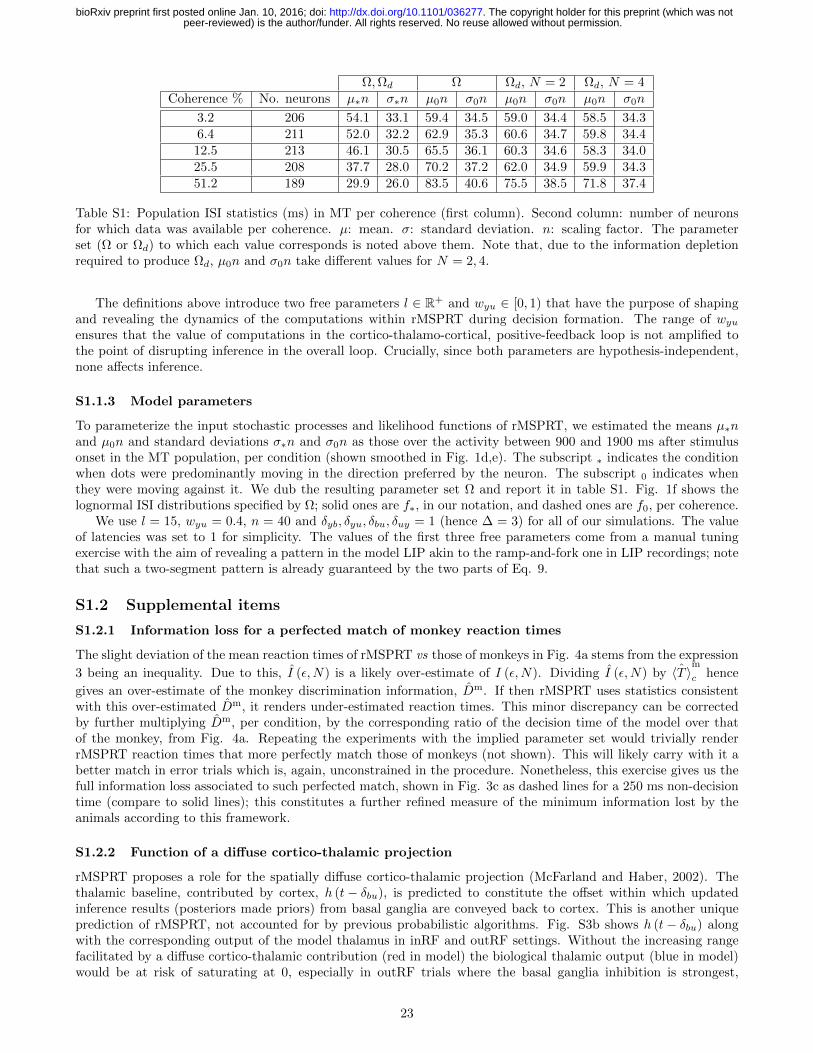
Ω,Ωd Ω Ωd, N = 2 Ωd, N = 4Coherence % No. neurons µ∗n σ∗n µ0n σ0n µ0n σ0n µ0n σ0n

3.2 206 54.1 33.1 59.4 34.5 59.0 34.4 58.5 34.36.4 211 52.0 32.2 62.9 35.3 60.6 34.7 59.8 34.412.5 213 46.1 30.5 65.5 36.1 60.3 34.6 58.3 34.025.5 208 37.7 28.0 70.2 37.2 62.0 34.9 59.9 34.351.2 189 29.9 26.0 83.5 40.6 75.5 38.5 71.8 37.4

Table S1: Population ISI statistics (ms) in MT per coherence (first column). Second column: number of neuronsfor which data was available per coherence. µ: mean. σ: standard deviation. n: scaling factor. The parameterset (Ω or Ωd) to which each value corresponds is noted above them. Note that, due to the information depletionrequired to produce Ωd, µ0n and σ0n take different values for N = 2, 4.

The definitions above introduce two free parameters l ∈ R+ and wyu ∈ [0, 1) that have the purpose of shapingand revealing the dynamics of the computations within rMSPRT during decision formation. The range of wyuensures that the value of computations in the cortico-thalamo-cortical, positive-feedback loop is not amplified tothe point of disrupting inference in the overall loop. Crucially, since both parameters are hypothesis-independent,none affects inference.

S1.1.3 Model parameters

To parameterize the input stochastic processes and likelihood functions of rMSPRT, we estimated the means µ∗nand µ0n and standard deviations σ∗n and σ0n as those over the activity between 900 and 1900 ms after stimulusonset in the MT population, per condition (shown smoothed in Fig. 1d,e). The subscript ∗ indicates the conditionwhen dots were predominantly moving in the direction preferred by the neuron. The subscript 0 indicates whenthey were moving against it. We dub the resulting parameter set Ω and report it in table S1. Fig. 1f shows thelognormal ISI distributions specified by Ω; solid ones are f∗, in our notation, and dashed ones are f0, per coherence.

We use l = 15, wyu = 0.4, n = 40 and δyb, δyu, δbu, δuy = 1 (hence ∆ = 3) for all of our simulations. The valueof latencies was set to 1 for simplicity. The values of the first three free parameters come from a manual tuningexercise with the aim of revealing a pattern in the model LIP akin to the ramp-and-fork one in LIP recordings; notethat such a two-segment pattern is already guaranteed by the two parts of Eq. 9.

S1.2 Supplemental items

S1.2.1 Information loss for a perfected match of monkey reaction times

The slight deviation of the mean reaction times of rMSPRT vs those of monkeys in Fig. 4a stems from the expression

3 being an inequality. Due to this, I (ε,N) is a likely over-estimate of I (ε,N). Dividing I (ε,N) by ˆ〈T 〉m

c hence

gives an over-estimate of the monkey discrimination information, Dm. If then rMSPRT uses statistics consistentwith this over-estimated Dm, it renders under-estimated reaction times. This minor discrepancy can be correctedby further multiplying Dm, per condition, by the corresponding ratio of the decision time of the model over thatof the monkey, from Fig. 4a. Repeating the experiments with the implied parameter set would trivially renderrMSPRT reaction times that more perfectly match those of monkeys (not shown). This will likely carry with it abetter match in error trials which is, again, unconstrained in the procedure. Nonetheless, this exercise gives us thefull information loss associated to such perfected match, shown in Fig. 3c as dashed lines for a 250 ms non-decisiontime (compare to solid lines); this constitutes a further refined measure of the minimum information lost by theanimals according to this framework.

S1.2.2 Function of a diffuse cortico-thalamic projection

rMSPRT proposes a role for the spatially diffuse cortico-thalamic projection (McFarland and Haber, 2002). Thethalamic baseline, contributed by cortex, h (t− δbu), is predicted to constitute the offset within which updatedinference results (posteriors made priors) from basal ganglia are conveyed back to cortex. This is another uniqueprediction of rMSPRT, not accounted for by previous probabilistic algorithms. Fig. S3b shows h (t− δbu) alongwith the corresponding output of the model thalamus in inRF and outRF settings. Without the increasing rangefacilitated by a diffuse cortico-thalamic contribution (red in model) the biological thalamic output (blue in model)would be at risk of saturating at 0, especially in outRF trials where the basal ganglia inhibition is strongest,

23


http://dx.doi.org/10.1101/036277

Figure S1: Mapping of rMSPRT computations to the basal ganglia. Parallel computations for N hy-potheses —indexed by j— mapped onto the basal ganglia nuclei, within the grey dashed box (see Bo-gacz and Gurney (2007); Larsen et al. (2010); Bogacz and Larsen (2011)). Same conventions and nota-tion as in Fig. 5. All computations are delayed with respect to the substantia nigra pars reticulata.log∑Nk=1 exp (yk (t+ δyb) + logPk (t− δbu − δuy) + c (t+ δyb)): normalization term (from Eq. 13), putting together

the cortical computations for all hypotheses into a hypothesis-independent contribution. Note that the model stria-tum represents a copy of the cortical signal (as in Fig. 5) but its influence on the substantia nigra pars reticulatais the negative of such cortical input.

Figure S2: Qualitative prediction for the time course of striatum in rMSPRT. Same conventions as Fig. 7. (a)Aligned at decision initiation (Init; t = 1; dotted line). (b) Aligned at decision termination (Term; dotted line).Single Monte Carlo experiment with N = 2 and 800 total trials.

wasting then the segregation of hypotheses carried by it, represented by the fed-back posteriors in the model. Ifthe biological thalamus were thus saturated, rMSPRT also predicts that the cortex would be limited to producelikelihood-proportional responses only on the basis of the immediately incoming data, instead of making use of thewhole sequence.

Lastly, note that the increasing h (t− δbu) becomes h (t− δbu − δuy) at the model sensory-motor cortex. Thisis the time changing component of the cortical baseline, c (t+ δyb) (Fig. 5). Thus, we argue that h (t− δbu − δuy)may form part of the increasing choice-independent drive, dubbed “urgency signal”, revealed by Drugowitsch et al.(2012) when averaging population responses of LIP neurons during the dot motion task across choices, for separatecoherence levels.

24


http://dx.doi.org/10.1101/036277

Figure S3: Threshold in basal ganglia and influence of cortico-thalamic contribution. (a) Position of the threshold,θ, set at the model basal ganglia in simulations like those of Figs. 4, 6 and 7, per condition. (b) Example meancortico-thalamic contribution, h (t− δbu) (red), compared to the mean thalamic output in inRF settings (solid blue)and outRF ones (dashed blue) for 25 % coherence and N = 2. Both (a) and (b) come from single Monte Carloexperiments with 800, 1200 trials for N = 2, 4, respectively.

S1.2.3 Relation of rMSPRT to existing decision models

The predictions of rMSPRT on the anatomical mapping of computations, neural dynamics, behaviour and thestructure of the decision procedure in the brain, as explained here, are more comprehensive than those of priormodels of decision-making. Here we explain the relationship of rMSPRT to the major classes of decision models todate.

As said before, our rMSPRT generalizes the MSPRT (Baum and Veeravalli, 1994; Bogacz and Gurney, 2007)in allowing the re-use of posteriors at any given distance in the past as priors for present inference, via recursion.The MSPRT collapses (Baum and Veeravalli, 1994) to the sequential probability ratio test (SPRT) of Wald (1947)for N = 2 alternatives. The non-recursive Bayes’ rule in the first case of Eq. 9 is the MSPRT’s test statistic (usedby Eq. 14). Making a ratio of two such posteriors (i = 1, 2) gives a ratio of likelihoods times priors. If priors areflat, this gives a likelihood ratio, the original test statistic of SPRT; appropriate fixed thresholds and an equationanalogous to Eq. 14, complete the specification of SPRT. For N = 2, MSPRT is thus the physical, optimal limit ofperformance. The rMSPRT performs identically to MSPRT and so enjoys this same privilege. However, if made tocollapse in the same manner, the rMSPRT would produce a more flexible, recursive version of the SPRT allowingfor a corresponding re-use of posteriors as priors.

The popular drift diffusion model (DDM; e.g. Ratcliff (1978); Mazurek et al. (2003); Palmer et al. (2005); Dingand Gold (2010, 2012a, 2013); Brunton et al. (2013); Tsunada et al. (2016)) is a non-recursive version of the SPRT(strictly for N = 2). It is thus optimal and is related to rMSPRT in the aforementioned manner. The popularity ofthe DDM stems from it incorporating continuous time and stochasticity in its input —a time-continuous Gaussianprocess. Adding time-continuity added plausibility to the hypothesis that the brain somehow implements the SPRTfor decision (e.g. see Kira et al. (2015)), a problem also faced by the traditional discrete-time MSPRT. However,the existence of a Gaussian process in the brain to supply evidence for decisions, is unproven; since the the decisiontimes predicted by DDM critically hinge on this process and its statistics (typically disconnected from the statisticsof sensory neural activity), the interpretation of the DDM’s behavioural predictions is obscured. To solve all this,Caballero et al. (2015) introduced a continuous-time generalization of the MSPRT whose inputs consist of stochasticspike-trains —the natural format of data in the brain. Caballero et al. also demonstrated that, as an average, thisspiking MSPRT requires the same number of observations (inter-spike intervals) to decision as an equivalent instanceof the discrete-time, traditional MSPRT. This established a solid, formal link between the discrete neural informationused for decisions and the continuously distributed reaction times observed during behaviour. It also enabled usto interpret the discrete number of observations to decision in the simpler, discrete-time (r)MSPRT, as continuousdecision times. This link from spike-trains to behaviour is the first advantage of rMSPRT over DDM. A second,related advantage is the rMSPRT’s capability to relate choice behaviour to the statistics of the sensory data (spiketrains) that determines it, as showcased here. A third is that the rMSPRT predicts multiple decision variables,one per hypothesis; all decision variables drop (or grow in a linear space) towards a single threshold (although athreshold per decision variable can be set, see Baum and Veeravalli (1994); Caballero et al. (2015)) when theirassociated hypothesis is well supported by input data. This contrasts with the single decision variable driftingtowards one of two thresholds in the DDM and SPRT which has proven difficult to interpret neurobiologically.A fourth advantage is that (r)MSPRT is multi-alternative by design (N > 2), allowing us to analyse all realisticdecision settings with the same mechanism.

25


http://dx.doi.org/10.1101/036277

Usher and McClelland (2001) introduced a dynamical model where a decision variable per alternative affectsthose of all other alternatives via mutual inhibition. This model incorporates time-continuity, stochasticity andcompetition (like SPRT, DDM and (r)MSPRT) but also leakage, and allows for N > 2. It has been shown thatwhen leakage equals inhibition, the signal-to-noise ratio is set sufficiently low and N = 2, the Usher and McClelland(UM) model can approximate the DDM (SPRT) and achieve optimality (Bogacz et al., 2006; Bogacz and Gurney,2007). Further, Ditterich (2010) has demonstrated that feedback and feedforward mutual-inhibition configurationsperform equally, easing the constraints to map the UM model to brain circuits. From the UM model on we stepaway from hard statistical-inference algorithms (SPRT, DDM, (r)MSPRT) that aim at capturing biological decisionformation at an algorithmic level of description, towards a set of models aimed at the same at an implementationallevel. In so doing, we trade exact inference and the straightforward use of probability theory to learn about decisionformation for the gain of incorporating known neural properties (e.g. leakiness) and understanding how a biologicalneural network may implement decision (Beck et al. (2008) take important steps in this direction) and perhaps evenapproximate one of the hard, probabilistic algorithms, as shown here.

The last model we compare is the so-called Wang (2002) model and its extensions (e.g. Lo and Wang (2006);Wong et al. (2007); Furman and Wang (2008); Albantakis and Deco (2009)). Briefly, this is a biologically realisticimplementation of the UM model via populations of spiking neurons (Bogacz et al., 2006); thus, the Wang modelshares the UM model’s relationship to (r)MSPRT. The Wang model is a further, essential step towards understandingneural implementation. It is only at this level of description that the constraints of networks of spiking neuronstowards the execution of decision algorithms, fully manifest.

The road from algorithmic to neural implementation inevitably leads us to efficiency matters. Bogacz andGurney (2007) demonstrated that, given the same conditions the UM (hence Wang’s) model and the MSPRT(hence rMSPRT) can perform equally (optimally) for N = 2 but that MSPRT (thus rMSPRT) is much moreefficient for N > 2; this is, it requires less observations, hence shorter decision times, to make choices at the sameerror rate. Our research poses that the sluggish mean reaction times of monkeys can be accounted-for by a quasi-Bayesian observer (rMSPRT) ‘starved’ of sensory discrimination information. Altogether, this calls for furtherresearch on how to close the performance gap between implementation-close models such as UM’s and Wang’sand hard inference algorithms like rMSPRT. After all, implementing a decision procedure that is faster in general(N > 2) is highly desirable, making it a trait that evolution would be expected to have optimized in animals.

26


http://dx.doi.org/10.1101/036277

Documents

Evidence for a probabilistic, brain-distributed, recursive ... · Evidence for a probabilistic, brain-distributed, recursive mechanism for decision-making Javier A. Caballero 1 ;