Evidence-based sensor tasking for space domain … · Evidence-based sensor tasking for space domain awareness Andris D. Jaunzemis ... expert might be able to conﬁrm or refute a

Evidence-based sensor tasking for space domain awareness

Andris D. JaunzemisGraduate Research Assistant, Aerospace Engineering, Georgia Institute of Technology

Marcus J. HolzingerAssistant Professor, Aerospace Engineering, Georgia Institute of Technology

Moriba K. JahDirector, Space Object Behavioral Sciences, University of Arizona

Abstract

Space Domain Awareness (SDA) is the actionable knowledge required to predict, avoid,deter, operate through, recover from, and/or attribute cause to the loss and/or degradation ofspace capabilities and services. A main purpose for SDA is to provide decision-making pro-cesses with a quantifiable and timely body of evidence of behavior(s) attributable to specificspace threats and/or hazards. To fulfill the promise of SDA, it is necessary for decision makersand analysts to pose specific hypotheses that may be supported or refuted by evidence, someof which may only be collected using sensor networks. While Bayesian inference may supportsome of these decision making needs, it does not adequately capture ambiguity in supportingevidence; i.e., it struggles to rigorously quantify ‘known unknowns’ for decision makers. Overthe past 40 years, evidential reasoning approaches such as Dempster Shafer theory have beendeveloped to address problems with ambiguous bodies of evidence. This paper applies math-ematical theories of evidence using Dempster Shafer expert systems to address the followingcritical issues: 1) How decision makers can pose critical decision criteria as rigorous, testablehypotheses, 2) How to interrogate these hypotheses to reduce ambiguity, and 3) How to task anetwork of sensors to gather evidence for multiple competing hypotheses. This theory is testedusing a simulated sensor tasking scenario balancing search versus track responsibilities.

1 IntroductionSpace situational awareness (SSA) is concerned with accurately representing the state knowl-

edge of objects in the space environment to provide better prediction capabilities for threats suchas potential conjunction events. More recently, the discourse on SSA has turned toward spacedomain awareness (SDA), reflecting the ever-growing reality of world-wide space capabilities andthe impact that decisions in the space environment can have on a global relational scale. In partic-ular, SDA focuses on gathering actionable data to supply to decision-makers in their evaluation ofhypotheses [1]. The space community as a whole suffers from a problem of producing high quan-tities data (in the form of tracks) but being unable to produce significant data on any specific objector event to increase understanding of that event. Currently, there are over 20,000 trackable objectsin the space object catalog [2]. Due to observational constraints imposed by orbital mechanics,the limited number of space-observing sensors are unable to observe each object. This hindersthe ability to reliably provide information on maneuvers or other events in space. Therefore, more

1Copyright © 2016 Advanced Maui Optical and Space Surveillance Technologies Conference (AMOS) – www.amostech.com

emphasis is being placed on algorithms and processes that have an ability to ingest disparate datafrom many sources and fuse an understanding of the greater situation of the space domain.

In typical Bayesian reasoning, deterministic probabilities are placed on event hypotheses underthe assumption that the only possible realizations of this hypothesis are true or false. However,in complex decision-making contexts, information is not always best-represented in this strictlybinary manner, since some evidence for a particular hypothesis might also involve ambiguity. Anexpert might be able to confirm or refute a given set of hypotheses, but it cannot attribute belief toany hypotheses for which it is not an expert. For this reason, evidential reasoning methods, such asDempster-Shafer theory, quantify this ambiguity in situation knowledge, leading to more realisticmodeling of human analyst processes [3, 4].

The human-analyst-like approach to belief structures in Dempster-Shafer theory and the decision-making focus of SDA make the pair a promising combination. SDA focuses on actionable knowl-edge required for operation in the space environment without loss or degredation of capabilitiesand services [1]. Decision-making in SDA ranges from collecting raw observables, to identify-ing space object properties such as orbit state, to inferring mission types and evaluating specificthreats [1]. Given this “big-data” problem, decision-makers must form hypotheses about the envi-ronment and its constituent objects, and apply available data to evaluate these hypotheses. Currenttechniques focus largely on collecting observables, identification of physical states and parame-ters, and determining functional characteristics [1]. For instance, some tasking techniques simplyaim to maximize the number of collections in a given time horizon, whereas others might focuson minimizing covariance in the state estimates [5] Recent improvements in these data collectiontechniques include the use of Finite Set Statistics in detection and tracking [6, 7] and the classi-fication approaches using ontologies and taxonomies [8]. Evidential reasoning has an ability toaugment the previous techniques by ingesting a wide range of SDA data (e.g. observational data,correlated tracks, classification results) as evidence that is used to directly interrogate hypothesesof interest to the decision-maker.

This paper begins by introducing relevant elements of evidence-based reasoning. A binary-hypothesis approach to individual hypothesis formulation is discussed to allow decision-makersto form rigorous, testable hypotheses. A mathematical framework for decision-making in SDAsensor tasking is developed to allow interrogation of these hypotheses on the basis of removingambiguity from the system. The application of this framework in a multi-objective framework isfurther developed since the subsets of the SDA problem are inherently multi-objective. Due to thecombinatorial nature of these problems, a toy example relevant to SDA is developed to demonstrateapplicability of this method in a reduced space.

2 TheoryIn this section begin by summarizing relevant aspects of Dempster-Shafer theory, introducing

terminology and notation that will be used throughout the paper. This is followed by a discussionon the relevance of ignorance in decision-making contexts, and further how decision-makers candecompose complex hypotheses into simple binary hypotheses to apply Dempster-Shafer effec-tively. Finally, we present the sensor tasking ignorance-based optimization methodology in Eqn.(11).


2.1 Dempster-Shafer TheoryDempster-Shafer (D-S) theory deals with the assignment of belief to particular hypotheses

based on available evidence. The set of hypotheses under consideration Θ = {θ1, θ2, . . .} is calledthe frame of discernment. In D-S theory, the hypotheses that comprise the frame of discernmentshould be mutually exclusive and collectively exhaustive; in other words, exactly one of thesehypotheses must be true at a given instant.2.1.1 Basic Belief Assignments

Given a frame of discernment Θ, the function m, called the basic belief assignment (BBA),assigns belief values in the range 0 to 1 to a subset of hypotheses: m : θ 7→ [0, 1], θ ⊆ Θ. A BBArepresents an expert’s belief in each hypothesis based on the evidence available to that expert.BBAs are typically assumed to possess a few properties:

1)∑

A⊆Θ m(A) = 1

2) m(∅) = 0

The first property ensures that the support attributed to the hypotheses in the frame of discernmentadds up to 1. The second property enforces that belief is only attributed to hypotheses available inthe frame of discernment.

The set of hypotheses that have non-zero belief mass are the focal set of the associated BBA.For ease of discussion, a number of common BBAs are typically defined based on their focalsets. A vacuous BBA is one in which all the belief mass is assigned to Θ, such that m(Θ) = 1,m(A) = 0 ∀A ⊂ Θ. A simple BBA is one in which the focal set consists of only two elements:the entire frame of discernment Θ and one other hypothesis, as in m(A) = p, m(Θ) = 1 − p,m(B) = 0 ∀B ∈ 2Θ \ {A,Θ}.

Using BBAs, Shafer defines the notions of belief and plausibility, which form lower and upperbounds on the probability that a proposition is provable given the available evidence. Belief andplausibility can be computed from a given BBA m using Eqs. (1) and (2), respectively:

bel (A) =∑B⊆A

m(B) (1)

pl (A) =∑

B∩A6=∅

m(B) = 1− bel (¬A) (2)

where ¬A is the negation, or complement, of hypothesis A. In other words, the expert’s belief in,or support for, hypothesis A, is composed of the sum of the belief masses attributed to A and itssubsets. The plausibility of hypothesis A is composed of the sum of the belief masses attributedto any hypothesis whose intersection with hypothesis A is non-empty. Also note that, since thetruth-set Θ represents the disjunctive combination of an exhaustive set of hypotheses, the beliefand plausibility of the truth-set must both be equal to 1.2.1.2 Combination Rules

Numerous methods exist for combining BBAs from multiple experts to form a fused massfunction [9]. The new mass function behaves just like any other BBA, so a fused understandingof belief and plausibility can be obtained. Each combination method exhibits slightly differentproperties, so implementation should take into consideration use-cases of this fused belief and


characteristics of the evidence sources. A common BBA combination technique is Dempster’sconjunctive rule, which is commutative, associative, and admits the vacuous BBA. Dempster’sconjunctive rule of combination, shown in Eq. (3), is often represented using the ⊕ operator. Thebelief mass attributed to hypothesis A ⊆ Θ after combination of BBAs from experts i and j isgiven as:

mi⊕j (A) = (mi ⊕mj) (A) =

∑B∩C=Ami(B)mj(C)

1−K(3)

K =∑

B∩C=∅

mi(B)mj(C) (4)

where K is a term that accounts for conflict between the bodies of evidence. The use of theconflict term K in Eqn. (3) has the effect of attributing conflicting evidence to the null-set. Sincesupport cannot be attributed to the null-set (in classical Dempster-Shafer theory), this belief massis normalized across the remaining hypotheses [9].

Some uses of Dempsters rule lead to counter-intuitive results in the presence of extreme con-flict, an observation typically referred to as Zadehs paradox [10]. However, the scenario in Zadehsparadox can be resolved by more carefully adhering to Cromwells Rule, i.e. not assigning a prob-ability of exactly 0 or 1 to any particular prior. This caveat, with the inclusion of the open-worldassumption, i.e. admitting that the actual true event might lie outside the theorized set of pos-sible events, led to the development of the Transferable Belief Model (TBM) as a derivative ofDempster-Shafer theory [11]. The constraints of this particular application allow the classicalDempster-Shafer implementation to be appropriate without applying TBM.

It is important to note that Dempsters rule is not idempotent. Subsequent evidence is assumedto be statistically independent of previous evidence. Therefore, when using Dempsters rule, theevidence must be assumed to be distinct; otherwise, repeated evidence will be heavily weighted inthe fused belief mass.

Dempster’s rule is also not the only combination rule for BBAs. For instance, Yager developeda related class of combination rules that, like Dempster’s rule, are commutative and not idempotent,but in Yager’s case the rule is quasi-associative [12, 13]. The primary difference in Yager’s methodis the use of a separate probability structure, the ground probability assignment, to pool evidencebefore conversion to a BBA [9]. Instead of normalizing out conflict, evidence from conflictingevidence is attributed to the universal-set, the frame of discernment Θ. As such, Yager’s rule isalso called the unnormalized Dempster’s rule, and indeed in the case of no conflict both methodsyeild the same result [9].

Additional combination rules have been developed that do enforce idempotence, which can beemployed in the case of non-distinct bodies evidence. While the above methods are conjunctive(AND-based) in the attribution of evidence to hypothesis-intersections, alternate methods employdisjunctive (OR-based) to handle evidence from varying-reliability sources [9].

For a more complete discussion on important developments in Dempster-Shafer theory, Yagerand Liu compiled a book of classic works, reviewed by Dempster and Shafer, on the theory ofbelief functions [14].

2.2 Importance of IgnoranceDempster-Shafer and other evidential reasoning theories do not require an expert to report

belief in only singleton hypotheses. Instead, the focal set can contain any subset of the frame


of discernment, including the entire frame of discernment itself. This particular hypothesis isreferred to as the universal-set, so-called because it is, by definition, the disjunctive combinationof all the mutually exclusive and collectively exhaustive hypotheses. The hypothesis A = Θ issurely true; one of these hypotheses must have occurred given the exhaustive nature of the frameof discernment. However, attributing belief mass to Θ does not increase an analyst’s understandingof the situation. Instead, it represents a residual ambiguity, indicating that the expert was unable toattribute that belief to any particular hypothesis. This admits an ignorance on the part of the expertthat is crucial in modeling realistic decision-making environments.

Similarly, contributing belief to any non-singleton subset of hypotheses admits some ignorance(e.g. note the indeterminism in the statement ”I attribute X belief to either A or B”), since theexpert is saying it is unable to further delineate between those hypotheses based on its availableevidence. When considering potential courses of action, the ideal course leads to a state of perfectknowledge and no residual ambiguity; in other words, all belief is attributed solely to singletonhypotheses. This idea of ignorance is essential to our approach to tasking in SDA: to supportthe objectives of decision-makers, their hypotheses must be possible to interrogate with evidence,with the goal of confirming or rejecting the hypotheses. This can be alternately formulated asa minimization of ignorance in the hypothesis space. In a similar way that covariance-reductiontechniques aim to approach the truth of the estimated state (e.g. orbit) given the available data, atasking scheme focused on ignorance-reduction will yield the truth-or-falseness of that hypothesisgiven the available evidence.

2.3 Binary Hypothesis BBAsFrom Eqn. (3) It can be seen that the computational complexity of the combination of two

BBAs scales quadratically with the number of hypotheses in the frame of discernment. TheO(n2)nature of Dempster’s rule means it is computationally preferable to restrict the number of hypothe-ses n in Θ. The simplest and most computationally attractive frame of discernment is therefore abinary frame where the two hypotheses are simply a null and alternate hypothesis: Θ = {θ,¬θ}where the ¬ symbol indicates the negation of hypothesis θ. Using first order logic, a compli-cated frame of discernment an be decomposed into a number of subsets of frames, each addressingsmaller portions of information. The important aspect to consider is that the hypotheses beingformed must be able to be interrogated through data that is currently available or actionable. Therelevant action can then gather evidence to directly interrogate this hypothesis, feeding a BBA thatrepresents that particular expert.

Utilizing a binary hypothesis structure allows the combined BBA to be written simply:

Ki,j = mi(θ)mj(¬θ) +mi(¬θ)mj(θ) (5)

mi⊕j(θ) =mi(θ)mj(θ) +mi(θ)mj(Θ) +mi(Θ)mj(θ)

1−Ki,j

(6)

mi⊕j(¬θ) =mi(¬θ)mj(¬θ) +mi(¬θ)mj(Θ) +mi(Θ)mj(¬θ)

1−Ki,j

(7)

mi⊕j(Θ) =mi(Θ)mj(Θ)

1−Ki,j

(8)

Additionally, in this case, the ignorance in frame Θ associated with BBA m is simply the belief


attributed by m to the whole frame, since it is the only non-singleton hypothesis:

ig (Θ) = m(Θ) (9)

In the next section, we give an example of how BBAs can be constructed for some classic SDAsensors.

2.4 SDA Sensors as Dempster-Shafer ExpertsIn order to apply Dempster-Shafer reasoning, available SDA sensors must be cast as Dempster-

Shafer experts, using that sensor’s data as evidence to contribute belief mass to the available hy-potheses. In this paper, we are concerned with the tasking of electro-optical (EO) sensors suchas telescopes. A number of physical properties of the sensor must be provided for simulation,such as focal length and pixel size. Information on the observation environment is also availablein the form of cloud cover detection, sky brightness estimation, an observatory weather station,and local weather forecasting. This particular arrangement represents the available sensors for theGeorgia Tech observatory, which is home to the Georgia Tech Space Object Research Telescope(GT-SORT), a half-meter Raven-class telescope.

The radiometric model developed by Coder et al. [15] is used to compute the probability ofdetection of an RSO for a given EO sensor. To compute the probability of detection of an RSO foran EO sensor, the radiometric model in Eqn. (10), developed by Coder et al., is used [15]:

Pd (Isky, tratm) =1

2

[1− erf

(SNRalgσn − µso√

2σso

)](10)

where the relevant terms are: Isky background sky irradiance measured in(

mv

arcsec2

), tratm atmo-

spheric transmittance, SNRalg is the required SNR for a successful detection based on the chosendetection algorithm. The remainder of the terms and their methods of calculation are discussed atlength in [15]. Importantly, this model provides the ability to ingest information from the afore-mentioned sensors and form BBAs. Preliminary work [16] showed how sensors available at theGeorgia Tech Observatory, particularly an All-Sky camera and sky brightness monitor, could beused to fuse a better understanding of the observation environment, incorporating that real-timedata into the tasking algorithm through Eqn. (10). Using the probability from Eqn. 10 as belief inthe hypothesis that an object will be detected, for instance, the belief and ignorance can be pooledfor all sensors. This will be demonstrated in the simulated scenario below.

2.5 Ignorance-Based OptimizationIn the case that a decision-maker is only concerned with a single hypothesis, the above for-

mulation focused on minimizing ignorance can be implemented as a single-objective optimizationproblem. However, most interesting tasking problems occur where there are multiple competingobjectives, such as the “search vs track” scenario. In this case, allocation of sensor resources toaddress one objective will necessarily hinder progress in another objective.

One approach to multi-objective optimization involves the minimization of the weighted-sumof the competing objectives. This approach allows the decision-maker to specify the degree towhich he/she is concerned with a particular hypothesis and adjust tasking accordingly.

To formalize the optimization problem, let us define the set of all possible actions as A andthe set of all relevant hypotheses H. At a given epoch tk, each action Ai,k:k+1 acts on the currentunderstanding of the environmentHk to gather new information and update the relevant hypotheses


Figure 1: Search versus Track scenario illustration.

at the next time instant, Ai,k:k+1(Hk) 7→ Hk+1. The total sum of ignorance in the hypotheses Hk

can be calculated as ig (Hk) = ig (H1,k) + ig (H2,k) + . . . + ig (HN , k). Therefore, given a setof N weightings for N hypotheses W = {w1, w2, . . . , . . . N} the set of decisions Dk:k+M−1 ∈Ak:k+1×. . .×Ak+M−1:k+M taken from times tk, . . . , tk+M can be determined to minimize weightedtotal ignorance at the final time-step as follows:

W = {w1, w2, . . . , . . . N} (11)Ak:k+1 = {A1,k:k+1, A2,k:k+1, . . .}Hk = {H1,k, H2,k, . . . , HN,k}

Dk:k+M−1 ∈ Ak:k+1 × . . .×Ak+M−1:k+M

minDk:k+M−1

ig (Hk+N) =N∑i=1

wiig (Hi,k+N)

Varying the weights and re-evaluating the objective function generates a list of candidate solu-tions to minimize weighted total ignorance. The non-dominated points, with respect to ignorancein each individual hypothesis, form a pareto frontier [17]. That is to say, any point on that surfacecan be considered an optimal solution to this tasking problem.

Notice that the decision setDk:k+M−1 is an element from the Cartesian product of action spaces.It is this search space to find the optimal decision set that makes this problem, like the well-knownTraveling Salesman problem, NP-complete. The addition of a selection of weightings further in-creases the dimensionality of the problem, making long-time-horizon solutions with many differenthypotheses and actions computationally intractable. Therefore, the simulations in this paper willdeal with a simplified example that is computationally feasible at least in small time steps.

3 Simulation ResultsA search-versus-track simulation, illustrated in Fig. 3, is presented to evaluate the validity

and applicability of the theoretical results to realistic SDA scenarios. In this simulation, a singlesensor is tasked with tracking two space objects, one in low-Earth-orbit (LEO) and the other inGeostationary orbit (GEO). Additionally, the sensor is tasked to search for new space objects notalready in the catalog. Therefore, the decision-making process is a multi-objective optimizationproblem, trading between these three objectives (track object 1, track object 2, or search).


3.1 Hypothesis FormulationThe first step in applying Dempster-Shafer theory to this problem is to rigorously define hy-

potheses to be interrogated. In particular, we endeavor to formulate binary hypotheses to lessenthe computational burden in evidence combination and computing ignorance.3.1.1 Search

The goal of the search phase is to look for new space objects that are not in the space objectcatalog. The hypotheses can be stated simply as:

θS - An observation yields successful detection of a new space object.

¬θS - An observation does not yield successful detection of a new space object.

To provide evidence for search, a prior distribution is developed using space object catalogs.This is based of the assumption that an electro-optical sensor is Specifically, the Space-Track.orgcatalog is used for TLE data, and the Celestrak catalog is used for auxiliary space object data, suchas radar cross-section. The prior is computed by propagating the entire space object catalog fora simulated 24-hours, generating a sampling of unit-vectors in inertial space. A Gaussian kernel(with 10 m 1-sigma uncertainty) is convolved across each of the unit-vectors to form a probabilitydensity function (PDF) for the locations of space objects averaged over one day.

The PDF is further refined by accounting for observation conditions using Earth-shadow andsolar phase angle. Using a simple cylindrical Earth-shadow model [18], if the object is deemed tobe in Earth-shadow (both conditions met in Eqn. (12)) its probability density is zeroed out.

0 ≤ ‖rsun × xso‖ −RE (12)0 ≤ rsun · rso (13)

Similarly, solar phase angle φ (the angle formed by the space object and the sun from theperspective of the observer) is considered by scaling the mean of the relevant Gaussian componentby φ

180. If φ is near 0-degrees (space object directly between Earth and Sun), its probability density

is significantly discounted. These constraints ensure that the prior PDF of space objects includesonly those objects in good optical observation conditions. Finally, the PDF is transformed intolocal look-angle (azimuth-elevation) space for the observer at each simulation time epoch and re-normalized to include only those space objects above the horizon (elevation ≤ 0). The final PDFcan be interrogated to find the region of highest space object density to provide a region to search.

A sample contour plot of the PDF can be seen in Fig. 2 in two coordinate systems: rightascension-declination and azimuth-elevation. On these contours, the dark regions represent higherdensities of observable space objects. Note that the extreme declinations show the highest densitiesnear the poles, matching intuition for dense regions of space. The GEO belt also stands out at zerodeclination, though portions of the GEO belt are discounted due to solar phase angle. The azimuth-elevation data is shown in a polar plot, with the center representing 90-degrees elevation (directlyoverhead) and azimuth increasing clockwise from north at the top.

Now the prior PDF Ps can be used to provide evidence for the search hypotheses in planningthe sensor schedule. At each time step (t), the search region (az, el) with the highest space objectdensity is selected, yielding the following binary BBA for search, ms:

ms(θs) = Ps(t, az, el) , ms(¬θs) = 0 , ms ({θs,¬θs}) = 1− Ps(t, az, el) (14)


(a) Right-ascension and declination (b) Azimuth and elevation

Figure 2: Search prior PDFs based on space object catalogs

Note that the space object density at any given search area is typically very low (Ps(t, az, el) ≤≤1), so the amount of evidence gained (or ignorance lost) through a search action is similarly low.3.1.2 Track

The goal of the track phase is to track objects that are not in the space object catalog. Thehypotheses can be stated simply as:

θT - An observation yields successful detection of the tracked object.

¬θT - An observation does not yield successful detection of the tracked object.

The BBA for track is more complicated than that for search, since the θT hypothesis can bedecomposed into a number of parts. In order to guarantee successful detection, the space objectneeds to be visible (above the horizon), detectable (in favorable observation conditions), and itsposition uncertainty must be contained the field of view of the sensor.

Testing for visibility is straightforward: the space object elevation must be above a thresholdvalue based on the observing environment (e.g. 20 deg to clear the skyline in Atlanta):

Pv = 1 if el[t] >= elthreshold (15)= 0 else (16)

Detectability involves more effort to account for the local observation conditions, includingcloud cover and sky brightness. Equation (10) is used here again to compute the probability ofdetection, Pd, given the local conditions.

Finally, the uncertainty requirement enforces that the covariance remain within certain bounds.The associated probability is computed by determining the volume of the covariance ellipse that isintersected by the field of view after rotating the covariance into the observer’s frame.

Pc = 1 if covariance within FOV (17)

=Afov

Acov else(18)


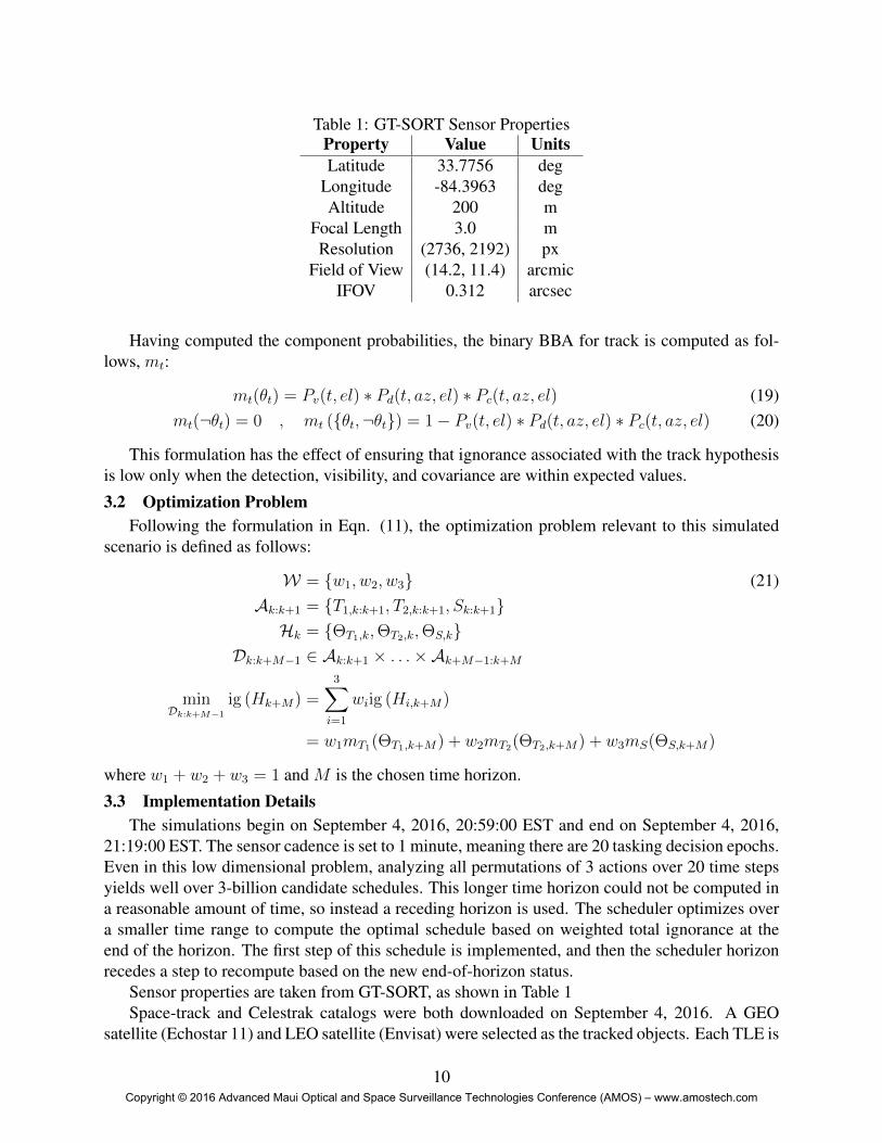
Table 1: GT-SORT Sensor PropertiesProperty Value UnitsLatitude 33.7756 deg

Longitude -84.3963 degAltitude 200 m

Focal Length 3.0 mResolution (2736, 2192) px

Field of View (14.2, 11.4) arcmicIFOV 0.312 arcsec

Having computed the component probabilities, the binary BBA for track is computed as fol-lows, mt:

mt(θt) = Pv(t, el) ∗ Pd(t, az, el) ∗ Pc(t, az, el) (19)mt(¬θt) = 0 , mt ({θt,¬θt}) = 1− Pv(t, el) ∗ Pd(t, az, el) ∗ Pc(t, az, el) (20)

This formulation has the effect of ensuring that ignorance associated with the track hypothesisis low only when the detection, visibility, and covariance are within expected values.

3.2 Optimization ProblemFollowing the formulation in Eqn. (11), the optimization problem relevant to this simulated

scenario is defined as follows:

W = {w1, w2, w3} (21)Ak:k+1 = {T1,k:k+1, T2,k:k+1, Sk:k+1}Hk = {ΘT1,k,ΘT2,k,ΘS,k}

Dk:k+M−1 ∈ Ak:k+1 × . . .×Ak+M−1:k+M

minDk:k+M−1

ig (Hk+M) =3∑i=1

wiig (Hi,k+M)

= w1mT1(ΘT1,k+M) + w2mT2(ΘT2,k+M) + w3mS(ΘS,k+M)

where w1 + w2 + w3 = 1 and M is the chosen time horizon.

3.3 Implementation DetailsThe simulations begin on September 4, 2016, 20:59:00 EST and end on September 4, 2016,

21:19:00 EST. The sensor cadence is set to 1 minute, meaning there are 20 tasking decision epochs.Even in this low dimensional problem, analyzing all permutations of 3 actions over 20 time stepsyields well over 3-billion candidate schedules. This longer time horizon could not be computed ina reasonable amount of time, so instead a receding horizon is used. The scheduler optimizes overa smaller time range to compute the optimal schedule based on weighted total ignorance at theend of the horizon. The first step of this schedule is implemented, and then the scheduler horizonrecedes a step to recompute based on the new end-of-horizon status.

Sensor properties are taken from GT-SORT, as shown in Table 1Space-track and Celestrak catalogs were both downloaded on September 4, 2016. A GEO

satellite (Echostar 11) and LEO satellite (Envisat) were selected as the tracked objects. Each TLE is


propagated using SGP4 through the simulation time range to compute the observation geometries.Covariances are propagated using an Extended Kalman Filter (EKF), with measurements gatheredin right-ascension declination space and measurement noise equal to the instantaneous field ofview (IFOV) of GT-SORT.

For the search hypothesis, the space object density prior is created using the downloaded cata-logs and averaged over September 4, 2016.

For simplicity of this report, equal weighting is applied across all three hypotheses.

3.4 Scenario: Clear Dark SkyIn this set of results, the sky brightness and cloud cover are both non-factors; the optical prob-

ability of detection is 1 throughout the simulation. The horizon- and covariance-based estimationsare still a factor, though, and affect the projected ignorance-loss due to the track actions.3.4.1 Greedy Optimization

The greedy optimization results in Fig. 4(a) show both computed optimal algorithm perfor-mance and a snapshot of the simulation in progress. The polar plots show azimuth (around cir-cumference, North at top) and elevation (radially outward, directly up at center) with the spaceobject density data superimposed over spacecraft tracks. Blue triangles indicate current position,and the red square indicates the sensor’s current action. The time-series data shows the scheduletaken at top and the ignorance in each hypothesis at each time step.

These results demonstrate an ability to reduce ignorance quickly. The GEO and Search areasare both detectable to start, but the ignorance reduction in the GEO observation is significantlygreater at step one, so it is chosen as the action. Further ignorance cannot be reduced in the GEOobservation, so the sensor switches to Search until the LEO object enters and satisfies the minimumelevation requirement. As the LEO object’s uncertainty evolves during propagation, its ignorancebegins to rise again as the covariance exceeds the field of view. Therefore, it is observed again,this time reducing a slightly different portion of the covariance due to the change in observationgeometry. Without a prediction horizon, however, this scheme oscillates between the remainingviable options for ignorance reduction (Search and Track LEO).3.4.2 5-step Horizon

In Figs. 4(b) and 4(c), we see the same initial schedule, ignorance, and spatial data from thegreedy tasking simulations. In the 5-step horizon case, the sensor performs similar to the greedyapproach until the LEO tracking phase. This time, it recognizes that it can minimize the LEOcovariance (and thereby the ignorance) at the end of the simulation by observing it at the lastpossible time step. This allows the sensor to continue to search for new objects and avoids the taskmode oscillation seen in the greedy approach.

3.5 Scenario: Dark Sky with CloudsThe final simulated data concerns a but dark night with clouds. Cloud cover is simulated in the

northern portion of the sky, where the LEO space object exits the field of view. The cloud-coveredgreedy simulation results have been omitted from this section since they are similar to the greedyresults in clear skies.3.5.1 5-step Horizon

Figure 4 shows the resulting cloudy night simulations. In good observation conditions, thealgorithm would want to get one more detection before the LEO object exits to minimize ignorancefrom the covariance expanding. However, here the sensor pivots to look for the LEO object earlier,


(a) Clear, greedy approach (Track LEO) (b) Clear, 5-step horizon (Search)

Figure 3: GT-SORT

just before it enters the cloudy skies. The remainder of the simulation is similar to the previous5-step horizon, checking GEO right away and remaining on the Search hypothesis the rest of thetime.

4 ConclusionsThis work applied Dempster-Shafer theory, with its ability to represent ambiguity to support

decision making, to SDA, with its emphasis on actionable information. Using first-order logic todecompose complicated hypothesis spaces into binary hypotheses, the decision-maker can createa computationally-tractable set of hypotheses to investigate. The optimization approach centersaround the minimization of ignorance in multiple competing objectives, providing a method oftasking that goes beyond gathering data and attempts to directly interrogate hypotheses throughsensor action. Simulated results of a seach-versus-track scenario show the algorithm is able tosuccessfully assign the sensor to track a set of objects based on the observation conditions, whilealso allocating resources to search for new objects.

Future work seeks to build upon this theory by applying multi-objective optimization tech-niques for quickly identifying non-dominated solutions in this vast decision space. The currentpaper used brute force to analyze all potential options, but ideally the current location on thepareto surface and its sensitivities to different decisions should lead the decision-maker to be ableto optimize the weighting schedule and gather much needed actionable data.

AcknowledgementsThis material is based upon work supported by the National Science Foundation Graduate

Research Fellowship under Grant No. DGE-1148903.


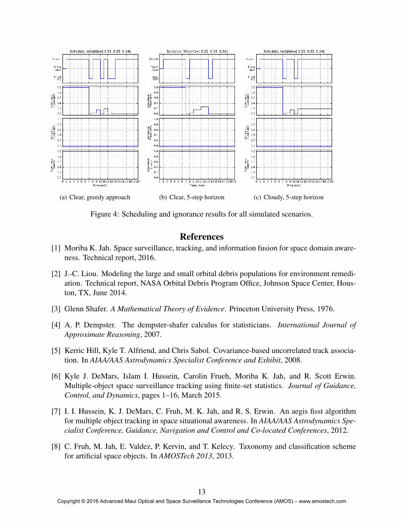
(a) Clear, greedy approach (b) Clear, 5-step horizon (c) Cloudy, 5-step horizon

Figure 4: Scheduling and ignorance results for all simulated scenarios.

References[1] Moriba K. Jah. Space surveillance, tracking, and information fusion for space domain aware-

ness. Technical report, 2016.

[2] J.-C. Liou. Modeling the large and small orbital debris populations for environment remedi-ation. Technical report, NASA Orbital Debris Program Office, Johnson Space Center, Hous-ton, TX, June 2014.

[3] Glenn Shafer. A Mathematical Theory of Evidence. Princeton University Press, 1976.

[4] A. P. Dempster. The dempster-shafer calculus for statisticians. International Journal ofApproximate Reasoning, 2007.

[5] Kerric Hill, Kyle T. Alfriend, and Chris Sabol. Covariance-based uncorrelated track associa-tion. In AIAA/AAS Astrodynamics Specialist Conference and Exhibit, 2008.

[6] Kyle J. DeMars, Islam I. Hussein, Carolin Frueh, Moriba K. Jah, and R. Scott Erwin.Multiple-object space surveillance tracking using finite-set statistics. Journal of Guidance,Control, and Dynamics, pages 1–16, March 2015.

[7] I. I. Hussein, K. J. DeMars, C. Fruh, M. K. Jah, and R. S. Erwin. An aegis fisst algorithmfor multiple object tracking in space situational awareness. In AIAA/AAS Astrodynamics Spe-cialist Conference, Guidance, Navigation and Control and Co-located Conferences, 2012.

[8] C. Fruh, M. Jah, E. Valdez, P. Kervin, and T. Kelecy. Taxonomy and classification schemefor artificial space objects. In AMOSTech 2013, 2013.


[9] Kari Sentz and Scott Ferson. Combination of evidence in dempster-shafer theory. Technicalreport, Systems Science and Industrial Engineering Department, Thomas J. Watson Schoolof Engineering and Applied Science, 2002.

[10] Lotif A. Zadeh. A simple view of the dempster-shafer theory of evidence and its implicationfor the rule of combination. AI Magazine, 7(2):85–90, 1986.

[11] Philippe Smets and Robert Kennes. The transferable belief model. Artificial Intelligence,66(2):191–234, 1994.

[12] Ronald R. Yager. Arithmetic and other operations on dempster-shafer structures. Interna-tional Journal of Man-Machine Studies, 25(4):357–366, 1986.

[13] Ronald R. Yager. On the dempster-shafer framework and new combination rules. InformationSciences, 41(2):93–137, 1987.

[14] Ronald R. Yager and Liping Liu. Classic Works of the Dempster-Shafer Theory of BeliefFunctions. Springer, 2008.

[15] Ryan D Coder and Marcus J Holzinger. Multi-objective design of optical systems for spacesituational awareness. Acta Astronautica, 2016.

[16] Andris D. Jaunzemis and Marcus J. Holzinger. Evidential reasoning applied to single-objectloss-of-custody scenarios for telescope tasking. In 26th AAS/AIAA Spaceflight MechanicsConference, February 2016.

[17] Garret N. Vanderplaats. Multidiscipline Design Optimization. Garret N. Vanderplaats, 2007.

[18] Adam C. Snow, III Johnny L. Worthy, Angela den Boer, Luke J. Alexander, Marcus J.Holzinger, and David Spencer. Optimization of cubesat constellations for uncued electroop-tical space object detection and tracking. Journal of Spacecraft and Rockets, 53(3):410–419,2016.


Documents

Evidence-based sensor tasking for space domain … · Evidence-based sensor tasking for space domain awareness Andris D. Jaunzemis ... expert might be able to conﬁrm or refute a