events - LIGOdhs/Amaldi03/cadonati.pdf · 5th Amaldi Conference LIGO-G0200XX-00-M Assigning a correlation confidence to a pair of coincident candidate events We suspect a burst happened

5th Amaldi ConferenceLIGO-G0200XX-00-M

Confidence test on waveform consistency in LIGO burst candidate

events

Laura CadonatiLIGO laboratory

Massachusetts Institute of Technology


Preface � The LIGO Burst Search pipeline uses Event Trigger Generators (ETGs) to flag times when

“something” occurs (burst candidates). Triggers from different interferometers are brought together in coincidence. All cuts in the pipeline are generous, in order to preserve sensitivity: we don’t really know what we are looking for…

� We want to use the full power of a coincident analysis: » What confidence can we put on the coincidence candidate?» Are the waveforms consistent? » Can we lower thresholds even further and dig deeper into the noise?

� The ETG outputs (∆t, BW, amplitude/power/SNR) do not provide enough information, weneed to go back to the time series

� Several options:» Cross correlation statistics (coherence) – Ref A. Weinstein, LIGO-G020401» Coherent power filter algorithm – Ref J. Sylvestre gr-qc/0304111» Time domain cross correlation

– Adopted by the External Trigger group (S. Marka et al.)– r-statistic test � subject of this talk


Assigning a correlation confidence to a pair of coincident candidate events

We suspect a burst happened in a 0.5 sec time window (order of 0.5-1 sec for TFCLUSTERS, tens of ms for SLOPE). We do not know:

what delay between the event at different sites (if any)how long the real event/burst is (1 ms?) when exactly it happens within the interval

� Load 5 sec of data from the two interferometers we want to cross-correlate, 2 sec before event start

� Decimate to Nyquist=2048Hz High-pass at 100 Hz� Whitening/line removal: train an adaptive filter over the first

second of loaded data, apply to the rest. This is fundamental to bypass the problem of non-stationary, correlated lines.

� Apply an r-statistic test to quote a confidence for the correlation


r-statistic

NULL HYPOTHESIS: the two (finite) series {xi} and {yi} are uncorrelated

⇒ Their linear correlation coefficient (Pearson’s r) is normally distributed around zero, with σ = 1/sqrt(N) where N is the number of points in the series (N >> 1)

S = erfc (|r| sqrt(N/2) ) Is the double-sided significance of the null hypothesis probability that |r| is larger than what measured, if {xi} and {yi} are uncorrelated

C = - log10(S) confidence that the null hypothesis is FALSE (that is: confidence that the two series are in fact correlated)

Linear correlation coefficient ornormalized cross correlation for the two series {xi} and {yi}


We shift one of the two series (one data point at a time) and calculate a series of:

coefficients rksignificances Skconfidences Ck

…then look for the maximum confidence.Shift limits: ±10 ms (LLO-LHO light travel time)

What delay?


CM = Max confidence = confidence in the correlation of the event pairτ = Time shift for max confidence = delay between IFOs


� Bandwidth:» This is a broadband correlation, effectively limited by the 100 Hz high-pass

filter and the initial decimation (2kHz low pass). » For a narrow band correlation, we are considering band-pass filters in pre-

process

� Integration time w:» If too small, we lose waveform information and the test becomes less reliable» If too large, we wash out the waveform in the cross-correlation

– Test different w and do an OR of the results!(Now considering: 20ms, 50ms, 100ms )

� Location within the trigger duration ∆T:» Partition trigger in M=ceil(2∆T/w)+1 subsets and calculate CM (wm) (m=1..M)» Use Γ = max(CM (wm)) as the ultimate confidence for the detector pair over

the whole event duration

How long?

When?



Event start Event stop

This procedure allows for bursts with separation up to 10 ms at any point within the trigger duration.

S2 hardware injection Feb 25, 2003 H1-L1 (sine gaussian, 361Hz, Q=9)

∆t= - 0.01 s ∆t= + 0.01 s

Divide in segments of duration τ

shift by +/- 10 ms and find CM (τm)

Move τ/2 forwards and get CM (τm+1)

Repeat until the whole event duration is covered


Event start Event stop

∆t= - 0.01 s ∆t= + 0.01 s

This procedure allows for bursts with separation up to 10 ms at any point within the trigger duration.

S2 hardware injection Feb 25, 2003 H1-L1 (sine gaussian, 361Hz, Q=9)

Divide in segments of duration τ

shift by +/- 10 ms and find CM (τm)

Move τ/2 forwards and get CM (τm+1)

Repeat until the whole event duration is covered


Comparing the {rk} distribution to the null hypothesis expectation

On a single sub-segment of width τ:

� Calculate the {rk} series (r-statistic)

� With a Kolmogorov-Smirnov test, we can compare the {rk} distribution to the null hypothesis expectation (normal distribution with σ=sqrt(1/N))

� α = 0.05 significance of the test» The {rk} series fails the test if the probability to get the measured distribution with uncorrelated

events is p<α

� If the test fails: the {rk} distribution is NOT consistent with the null hypothesis. In other words, it is “interesting”.

� We then move on to the calculation of the decimated confidence series and of CM (τm)


� L1-H1 r-statistic plots with integration time τ=20ms,centered at the (known) injection time.

� The r-statistic histogram is Gaussian, but with σobviously larger than what expected in the null hypothesis

� the Kolmogorov-Smirnov test can discard the null hypothesis

» (there is less than 0.1% probability that this distribution is due to uncorrelated series)

Plots to be updated (sine gaussian at 554 Hz, software inj.). Merge with previous slide.


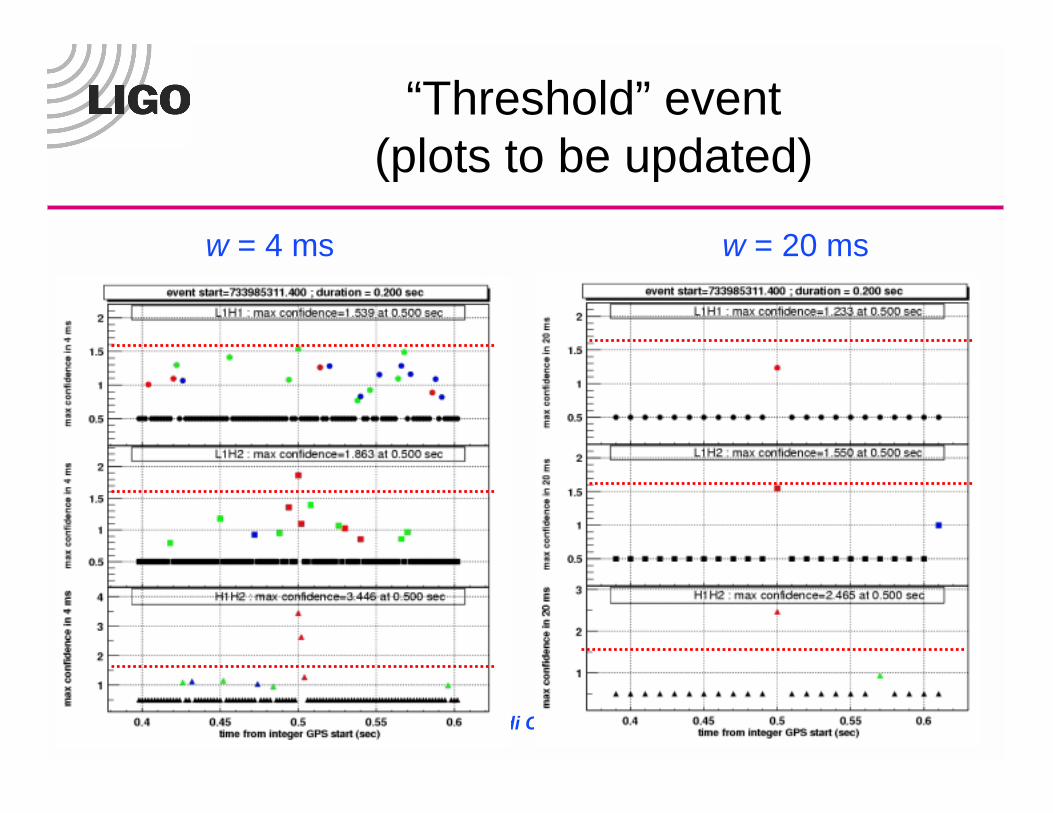
“Loud” event : CM(wm) plots

� Each point: max confidence CMfor an interval τ m (τ=20ms)

� Black: time interval τ m is uncorrelated, according to KS test with significance α = 5%

� Red: correlation cannot be excluded (interval fails KS test with 5% significance)

� Define a cut (pattern recognition?):

» 2 IFOs: Γ=max(CM(wm) ) > β2» 3 IFOs: Γ ij=max(CM(wm) ) > β3

simultaneously for each IFO pair » In general, we can have β2 ≠ β3≈ β=3: 99.9% correlation probability

Γ=max(CM(wm) )

CM(wm) plots at the three pairs of IFOs


backgroundThreshold


Gaussian injections (3e-19 and 1e-18 peak strain)


“Threshold” event (plots to be updated)

w = 4 ms w = 20 ms


Software injections: Sine Gaussians f0=554 Hz Q=9

Background(no injection): no

falses if b3=3

0.75 h_0Below ETG threshold ;50% efficiency

h_0ETG at 50%; xx% efficiency

3 h_0


Outlook

r-statistic test for cross correlation in time domain:» Assigns a confidence to coincidence events at the end of the burst

pipeline.» Verifies the waveforms are consistent » Reduces false rate in the burst analysis, allowing for lower thresholds

In progress:» Method tuned on hardware injections.» Ongoing investigation with software injections (gaussians, Zwerger-

Mueller)» Exploring filter optimization and improved timing information

Documents

events - LIGOdhs/Amaldi03/cadonati.pdf · 5th Amaldi Conference LIGO-G0200XX-00-M Assigning a correlation confidence to a pair of coincident candidate events We suspect a burst happened