FINALCONTRACT REPORT

EVALUATION OF TRAFFIC SIGNALTIMING OPTIMIZATION METHODS

USING A STOCHASTIC AND MICROSCOPICSIMULATION PROGRAM

B. BRIAN PARK, Ph.D.Research Assistant Professor

Department of Civil EngineeringUniversity of Virginia

J. D. SCHNEEBERGERGraduate Research Assistant

V·I·R·G·I·N· I·A

TRANSPORTATION RESEARCH COUNCIL

VIRGINIA TRANSPORTATION RESEARCH COUNCIL

1. Report No.FHWA/VTRC

Standard Title Page - Report on Federally Funded Project2. Government Accession No. 3. Recipient's Catalog No.

4. Title and SubtitleEvaluation of Traffic Signal Timing Optimization Methods UsingA Stochastic and Microscopic Simulation Program

7. Author(s)Brian Park and J.D. Schneeberger

9. Performing Organization and Address

Virginia Transportation Research Council530 Edgemont RoadCharlottesville, VA 22903

5. Report DateNovember 20026. Performing Organization Code

8. Performing Organization Report No.

10. Work Unit No. (TRAIS)

11. Contract or Grant No.57935

12. Sponsoring Agencies' Name and Address

Virginia Department of Transportation1401 E. Broad StreetRichmond, VA 2321915. Supplementary Notes

16. Abstract

FHWAP.O. Box 10249Richmond, VA 23240

13. Type of Report and Period CoveredFinal:February 2001 - September 200214. Sponsoring Agency Code

This study evaluated existing traffic signal optimization programs including Synchro, TRANSYT-7F, and genetic algorithmoptimization using real world data collected in Virginia. As a first step, a microscopic simulation model, VISSIM, was extensivelycalibrated and validated using field data. Multiple simulation runs were then made for signal timing plans such that drivers'behavior, day-to-day traffic variation, etc were considered in the evaluation. Finally, long-term demand growth or changes werestatistically modeled and evaluated, again using multiple simulation runs.

Five timing plans were evaluated using the simulation test bed: 1) VDOT's former timing plan, 2) VDOT's current timing plan, 3)the genetic algorithm optimized timing plan, 4) the Synchro optimized timing plan, and 5) the TRANSYT-7F optimized timing plan.The simulation study results indicated that the current practice of VDOT signal optimization procedure significantly improves uponits former one by reducing travel times by 17% and total system delay by 36%. The three "optimized" timing plans did not providesignificant improvements.

Evaluation of the Lee Jackson Memorial Highway network showed that the current VDOT signal optimization proceduresignificantly improved the performance of network operations. Thus, the study recommended that VDOT continue using itsprocedure for developing new timing plans, but that it evaluate its signal timing plan regularly so that it does not become outdated.

17 Key WordsTraffic Signal OptimizationStochastic Simulation ModelSimulation Model Calibration and Validation

18. Distribution StatementNo restrictions. This document is available to the public throughNTIS, Springfield, VA 22161.

19. Security Classif. (of this report)Unclassified

20. Security Classif. (of this page)Unclassified

21. No. of Pages33

22. Price

Form DOT F 1700.7 (8-72) Reproduction of completed page authorized

FINAL CONTRACT REPORT

EVALUATION OF TRAFFIC SIGNAL TIMING OPTIMIZATION METHODS USINGA STOCHASTIC AND MICROSCOPIC SIMULATION PROGRAM

B. Brian Park, Ph.D.Research Assistant Professor

Department of Civil EngineeringUniversity of Virginia

J. D. SchneebergerGraduate Research Assistant

Project ManagersMichael A. Perfater, Virginia Transportation Research Council

Catherine C. McGhee, Virginia Transportation Research Council

Contract Research Sponsored bythe Virginia Transportation Research Council

Virginia Transportation Research Council(A Cooperative Organization Sponsored Jointly by the

Virginia Department of Transportation andthe University of Virginia)

Charlottesville, Virginia

January 2003VTRC 03-CR12

NOTICE

The project that is the subject of this report was done under contract for the VirginiaDepartment of Transportation, Virginia Transportation Research Council. The contentsof this report reflect the views of the authors, who are responsible for the facts and theaccuracy of the data presented herein. The contents do not necessarily reflect theofficial views or policies of the Virginia Department of Transportation, theCommonwealth Transportation Board, or the Federal Highway Administration. Thisreport does not constitute a standard, specification, or regulation.

Each contract report is peer reviewed and accepted for publication by Research Councilstaff with expertise in related technical areas. Final editing and proofreading of thereport are performed by the contractor.

Copyright 2003 by the Commonwealth of Virginia.

11

ABSTRACT

Traffic signal timing optimization has been recognized as one of the most cost-effectivemethods for improving mobility within the urban transportation system. Inappropriate signaltiming plans can cause not only discomfort (extra delay) to drivers but also increased emissionsand fuel consumption. Thus, it is important to investigate the practice of signal optimizationmethodology to ensure that newly developed timing plans will improve the system performance.The investigation can be conducted via either field testing or the use of a reliable simulation tool.Due to the risk and time requirements of field testing, simulation tools are being widely used.However, simulation models must be properly calibrated and validated so that the model outputcan be trusted.

This study evaluated existing traffic signal optimization programs including Synchro,TRANSYT-7F, and genetic algorithm optimization using real-world data collected in Virginia.As a first step, a microscopic simulation model, VISSIM, was extensively calibrated andvalidated using field data. Multiple simulation runs were then made for signal timing plans suchthat drivers' behavior, day-to-day traffic variation, etc. were considered in the evaluation.Finally, long-term demand growth or changes were statistically modeled and evaluated, againusing multiple simulation runs.

Five timing plans were evaluated using the simulation test bed. The timing plans underevaluation included (1) the former timing plan of the Virginia Department of Transportation(VDOT), (2) VDOT's current timing plan, (3) the genetic algorithm optimized timing plan, (4)the Synchro optimized timing plan, and (5) the TRANSYT-7F optimized timing plan. Thesimulation study results indicated that the current practice of VDOT' s current signal optimizationprocedure significantly improved upon its former one by reducing travel times by 17% and totalsystem delay by 36%. The three "optimized" timing plans did not provide significantimprovements.

Evaluation of the Lee-Jackson Memorial Highway network showed that the currentVDOT signal optimization procedure significantly improved the performance of networkoperations. Thus, the study recommended that VDOT continue using its procedure fordeveloping new timing plans but that it evaluate its signal timing plan regularly so that it doesnot become outdated.

iii

FINAL CONTRACT REPORT

EVALUATION OF TRAFFIC SIGNAL TIMING OPTIMIZATION METHODS USINGA STOCHASTIC AND MICROSCOPIC SIMULATION PROGRAM

B. Brian Park, Ph.D.Research Assistant Professor

Department of Civil EngineeringUniversity of Virginia

J. D. SchneebergerGraduate Research Assistant

INTRODUCTION

A great deal of effort has been dedicated to the design of better traffic signal timing plansfor the last four decades, but very little research has been conducted in the evaluation of signaltiming plans, especially in the context of stochastic and microscopic simulation environments.Furthermore, stochastic and microscopic simulation-based signal optimization has been verylimited mainly due to heavy computational burden. Thus, the state of the practice has been touse programs including TRANSYT-7F, Synchro, and PASSER-II to optimize traffic signaltiming plans based on the embedded macroscopic simulation models. With advances incomputation technology, the use of microscopic simulation becomes more feasible. Thus, anoptimization and evaluation of traffic signal timing plans based on stochastic and microscopicsimulation seems very natural since the urban street network itself contains a variety ofstochastic aspects including different drivers' behavior, vehicle mix, and day-to-day demandvariations. The use of deterministic and macroscopic simulation-based signal optimizationmethods could easily result in a local optimum or even a poor solution. A recent study alsoindicates that a signal timing plan based on a direct signal optimization using a stochastic andmicroscopic simulation model produces better performance than that of a macroscopicsimulation-based method (Rouphail et aI., 2000). The similar study also indicated that the use ofa well-calibrated simulation program is crucial in the evaluation of signal timing plans (Park etaI., 2001).

It is often practical to use a computer simulation model in evaluating a newly developedtraffic signal timing plan before its actual field implementation. The value of a stochasticsimulation model is its ability to account for system variability through repeated model runs. If asufficient number of runs are conducted, the daily variations in traffic flow can be factored intothe results. Even though a few researchers have used stochastic and microscopic simulationprograms for such purposes, the issue of variability was not well addressed in their efforts. Insome cases, the number of replications is relatively small such that the distribution of systemperformance was not investigated. At times, with a highly variable system, the results (usuallythe mean of system performance) could be misleading if only a small number of replicationswere used. This project develops and uses the distribution of system performance in evaluatingthe performance of traffic signal timing plans. It is important to investigate system performance

with respect to not only the mean value but also its variability. It might be advantageous toimplement a timing plan that produces a slightly higher average system delay with tighter delayvariations than a plan that yields a lower average system delay with higher system delayvariations. For example, a timing plan that produces the average system delay of 32 seconds pervehicle with a standard deviation of 5 should be implemented rather than a timing plan thatproduces the average system delay of 28 seconds per vehicle with a standard deviation of 10.

When a new timing plan is evaluated via a stochastic and microscopic computersimulation program, demand fluctuations are usually discarded. Even though multiple runs ofstochastic simulation produce random variability, they do not account for significant demandfluctuations. When the evaluation of a signal timing plan is conducted in an area such asNorthern Virginia, demand fluctuations ought to be carefully considered. A simple Monte Carlosimulation, one of the most common simulation methods, could be used to account for suchdemand fluctuations. However, this would require a significant amount of resources and mightnot be practical. This project uses an advanced statistical method so that demand fluctuations aresystematically considered in an efficient manner.

PURPOSE AND SCOPE

The purpose of this study was to evaluate current signal optimization methods. Theinvestigated methods included Synchro, TRANSYT-7F, and genetic algorithm optimization. Itwas anticipated that the evaluation would yield the following:

•

•

•

calibrated input parameters based on field data collected in Virginia for a stochastic andmicroscopic simulation program tested in this study

a well-calibrated traffic signal evaluation test bed

a methodology that can evaluate the distribution of system performance of a newlydeveloped traffic signal timing plan for various demand and input conditions before its actualfield implementation.

Case studies used in the evaluation of simulation optimization methods were confined to the test­bed network consisting of 12 signalized intersections along Route 50 in Northern Virginia.

METHODS

The research approach in this study involved (1) a literature review, (2) development of atest bed, (3) calibration and validation of the simulation model, and (4) signal timing planoptimization and evaluation.

2

Literature Review

Literature was reviewed the current practices in the simulation model calibration andvalidation, traffic signal optimization programs (e.g., Synchro, TRANSYT-7F, and GeneticAlgorithm approach), and current optimizations practices.

Test Bed Development

Site Selection

The test site was chosen with the help of Northern Virginia Smart Traffic Signal Systempersonnel. The research team made site visits before making final decisions.

Data Collection

Data collection was required to provide simulation program input parameters and outputmeasures of performance for the calibration and validation of the microscopic simulation model.Some data were provided from VDOT plans; other data were collected directly from the field.

The geometric characteristics of the test network were obtained from a Synchro file usedby VDOT. Distances between intersections, lengths of left- and right-tum lanes, intersectiongrades, detector locations, and speed limits were collected from this file. The timing plan fromthis file was also taken. This timing plan was labeled as the "base" timing plan, the timing planused by VDOT before it implemented its new timing plan, which was determined using Synchro.The signal timing plan currently used by VDOT in the field (referred to as the "field" timingplan) for the 12 intersections were extracted from the Management Information System forTransportation (MIST) terminal located in the Smart Travel Laboratory at the University ofVirginia. This system is directly linked to the timing plans used in the field at the test site andtherefore gives real-time data. Phases, splits, minimum green times, offsets, and gap out timeswere all taken from the system and used modeling in the microscopic simulation model, calledVISSIM (2001).

Although the MIST system terminal provided detector data, turning movement counts,especially for shared lane approaches, had to be collected in the field. The MIST systemterminal provides 15-minute local and system detector data on most approaches in the testnetwork, but not all of them. Additionally, the unreliability of traffic volume counts from loopdetectors made field collections of volumes a necessity. Both manual and video counts wereconducted in the field along the test network. Counts were collected on a normal weekday,Wednesday, July 11,2001, between 4:45 p.m. and 6:15 p.m.

A group of 16 people performed simultaneous manual counts along the test network.Manual counts were conducted at locations along the test site where detector data from MISTwere not suitable or obtainable. In order to use the data collected from the manual countssimultaneously with the MIST data, synchronization between clocks used by the manualcounters and the clock at the MIST system was performed before data collection. Shared laneapproaches were counted manually since loop detectors cannot distinguish between turning and

3

through movements. Manual counts were also conducted where there were no loop detectors orwhere the loop detectors were not working properly.

Four PATH dual cameras were used to conduct the video counts. These cameras,provided by VDOT, are a pole-mounted video system. The cameras were positioned on Lee­Jackson Memorial Highway at the intersections of Highland Oaks Drive, Intel Country ClubRoad, Stringfellow Road, and Lees Comer Road, where they recorded traffic conditions at theintersections.

The videotapes of these intersections were used to obtain accurate volume counts andturning percentages along the arterial and local streets. These video counts are more accuratethan manual or loop detector-based MIST counts for several reasons. Manual counts involvesome human error, especially when a counter is required to observe more than one movement athigh volumes. Since counters are observing at real time, it is possible that they may miss somevehicles when conducting counts. For example, it was often the case that manual countersmissed right-on-red counts because they were busy watching other movements. Loop detectordata on congested arterials do not always prove to be accurate either. Thresholds for monitoringa vehicle's presence are not always accurately set. As a result, volumes can be either over- orunderestimated depending on how the threshold for determining a vehicle's presence is set.Accuracy in video counts is possible mainly because the viewer may view the videotape morethan once. Therefore, the viewer can concentrate on a single movement and then, when finished,can review the tape and observe a different movement.

Eastbound leftmost lane travel times on Lee-Jackson Memorial Highway were used as ameasure of performance for the calibration process. This measure of performance was selectedbased on the ease of data collection from the field and output results from microscopicsimulation program. A direct comparison could easily be made between the field travel timesand simulation travel times.

Travel times were determined from two cameras with synchronized clocks that werepositioned on the bridges of Sully Road and Fairfax County Parkway overlooking the test site.The cameras were focused on the license plates of vehicles traveling in the leftmost lane alongLee-Jackson Memorial Highway and recorded a vehicle's license plate number when it enteredand left the test network. License plate numbers and times were recorded for every vehicle at thebeginning and end of the network and later matched. Subtracting the time the vehicle left thenetwork from the time the vehicle entered gave the vehicle's eastbound travel time in theleftmost lane.

The Smart Travel Laboratory Van, which uses an AUTOSCOPE video detection system,was used to measure and collect queue lengths, the validation measure of performance. Queuelengths were collected on a weekday in August 2001 so they could be used as an untried data setfor the validation process. The van was parked along the shoulder of Lee-Jackson MemorialHighway between the intersections of Muirfield Lane and Intel Country Club Road. The vanprovided video of a small segment of Lee-Jackson Memorial Highway between the twointersections. Queue lengths in the eastbound direction on the highway were collected from the

4

van's videotape by counting the number of vehicles in a queue at the end of red time for eachcycle during the data collection period.

Simulation Program and Network Coding

Microscopic Simulation Model: VISSIM

A stochastic and microscopic program, VISSIM (VISSIM, 2001), was chosen for thisstudy because it provides application programming interface (API) and powerful 3D animations.VISSIM version 3.50 is a microscopic simulation model with similar structures and capabilitiesas CORSIM (CORSIM, 1997). VISSIM is a microscopic, time step, and behavior-basedsimulation model. The model was developed at the University of Karlsruhe, Germany, duringthe early 1970s. Commercial distribution of VISSIM began in 1993 by PTV Transworld AG,who continues to distribute and maintain VISSIM today.

Essential to the accuracy of a traffic simulation model is the quality of the actualmodeling of vehicles or the methodology of moving vehicles through the network. In contrast toless complex models using constant speeds and deterministic car following logic, VISSIM usesthe psychophysical driver behavior model developed by Wiedemann in 1974 (VISSIM, 2001).The basic concept of this model is that the driver of a faster moving vehicle starts to decelerate ashe or she reaches his or her individual perception threshold to a slower moving vehicle. Sincethe driver cannot exactly determine the speed of that vehicle, his or her speed will fall below thatvehicle's speed until he or she starts to slightly accelerate again after reaching another perceptionthreshold. This results in an iterative process of acceleration and deceleration. Stochasticdistributions of speed and spacing thresholds replicate individual driver behavior characteristics.The model has been calibrated through multiple field measurements at the Technical Universityof Karlsruhe, Germany.

The basic idea of the Wiedemann model is the assumption that a driver can be in one offour driving modes:

1. Free Driving: No influences of preceding vehicles are observable. In this mode the driverseeks to reach and maintain a certain speed, his or her individually desired speed. In reality,the speed in free driving cannot be kept constant but oscillates around the desired speed dueto imperfect throttle control.

2. Approaching: The process of adapting the driver's own speed to the lower speed of apreceding vehicle. While approaching, a driver applies a deceleration so that the speeddifference of the two vehicles is zero in the moment he or she reaches his or her desiredsafety distance.

3. Following: The driver follows the preceding car without any conscious acceleration ordeceleration. He or she keeps the safety distance more or less constant, but again due toimperfect throttle control and imperfect estimation, the speed difference oscillates aroundzero.

5

4. Braking: The application of medium-to-high deceleration rates if the distance falls below thedesired safety distance. This can happen if the preceding car changes speed abruptly or if athird car changes lanes in front of the observed driver.

For each mode, the acceleration is described as a result of speed, speed differencebetween the follower and leader, distance between the follower and leader, and the individualcharacteristics of driver and vehicle. The driver switches from one mode to another as soon ashe or she reaches a certain threshold that can be expressed as a combination of speed differenceand distance. For example, a small speed difference can be realized in only small distances,whereas large speed differences are apparent and require drivers to react much earlier. Theability to perceive speed differences and to estimate distances, as well as the desired speeds andsafety distances, varies among the driver population. Because of the combination ofpsychological aspects and physiological restrictions of the driver's perception, the model iscalled a psychophysical car-following model.

Network Coding

The test site was coded in VISSIM Version 3.50 using the data collected from the fieldand VDOT information. The VISSIM model consists of two components: a simulator and signalstate generator. The simulator is responsible for generating traffic and is where the network isgraphically built. An aerial photograph of the study area was imported into the simulator. Thenetwork was then "digitized" over the aerial photograph, and attributes from the data collectionwere applied (e.g., lane widths, speed zones, detector locations). Although links are used in thesimulator, VISSIM does not have a traditional node structure. This link-based structure allowsflexibility to control traffic operation (e.g., yield conditions) and vehicle paths within anintersection.

The signal state generator is separate from the simulator and is where signal logicpresides. Signal control logic is input here for each intersection as VAP (vehicle actuatedprogramming) files. In these VAP files, signal characteristics are entered for the actuated signalsincluding phase sequences, minimum green times, force-offs, and gap out times. The signal stategenerator reads detector information from the simulator every time step. The signal stategenerator decides the signal display during a time step based on the detector information.

Model Calibration and Validation

Individual parameters in VISSIM were adjusted or tuned so that the model accuratelyrepresented field measured or observed traffic conditions. An eight-step calibration andvalidation procedure was decided upon:

Determination ofMeasures ofEffectiveness

The first step was to determine measures of effectiveness appropriate for calibration andvalidation. Performance measures, uncontrollable input parameters, and controllable inputparameters were identified. It was important to identify all measures of effectiveness clearlybefore proceeding forward in the calibration and validation process.

6

Identification of Calibration Parameters

All calibration parameters within the microscopic simulation model were identified, andacceptable ranges for each of the calibration parameter were determined.

Experimental Design for Calibration

The number of combinations among feasible controllable parameters is too large suchthat possible scenarios cannot be evaluated in a reasonable time. A Latin hypercube designalgorithm was used to reduce the number of combinations of calibration parameter scenarios.

Multiple Runs

In order to reduce stochastic variability, multiple runs were conducted for each scenariofrom the experimental design. The average performance measure and standard deviation wererecorded for each of the runs.

Development ofa Surface Function

A surface function, using the calibration parameters and measure of performance, wascreated from the results of the multiple runs.

Determination ofParameter Sets Based on Surface Function

The purpose of this step was to find an optimal parameter set that provides a close matchwith the field performance measure. Due to the fact that there could exist several parameter setsproviding output close to the target (i.e., field performance measure), several parameter sets wereconsidered.

Evaluation ofParameter Sets

Multiple runs were conducted to verify whether the parameter sets identified in theprevious step generate statistically significant results. For each parameter set, a distribution ofperformance measure was developed and compared with the field measure. Visualization wasalso used to evaluate the models.

Collection ofNew Data Setfor Validation

In order to validate the microscopic simulation model a new set of field data underuntried conditions was collected. The "calibrated" model was then evaluated with the new dataset.

7

Signal Timing Plan Optimization and Evaluation

Three traffic signal optimization tools were used to optimize the offsets on Lee-JacksonMemorial Highway: (1) linking a genetic algorithm (GA) to the calibrated VISSIM model, (2)coding and optimizing the network in Synchro, and (3) coding and optimizing the test site inTRANSYT-7F. The Synchro and TRANSY-7F optimizations were straightforward. The testnetwork was coded into the programs and optimized. The experimental setup for the GAoptimization worked as follows:

• The GA code developed in Fortran 90 language is linked to VISSIM using Rexx(Cowlishaw, 1990), a script language-based computer program.

• Signal timing plans (offsets) in binary representation form are randomly produced in the GA.The Rexx code converts the timing plans into integer values and inserts them directly into aVISSIM input file.

• VISSIM makes multiple runs (four or eight per timing plan) and outputs travel times for eachrun as *.rsr files.

• A second Rexx code extracts the performance measure (eastbound and westbound traveltimes) for each signal plan from the corresponding VISSIM output file (*.rsr). The Rexx filetakes a weighted average of travel times on Lee-Jackson Memorial Highway.

• The performance measures from the Rexx program are fed back to the GA. The GAevaluates the performance measures (attempts to minimize travel time) and then generates anew set of signal timing plans (offsets).

• The new timing plans are sent back to VISSIM where the process continues until all signaltiming plans proposed by the GA optimizer are run.

Traffic signal timing plans were evaluated using the calibrated VISSIM test network asan unbiased evaluator. Five timing plans were under investigation and include (1) VDOT'sformer timing plan, (2) VDOT's current timing plan, (3) the genetic algorithm optimized timingplan, (4) the Synchro optimized timing plan, and (5) the TRANSYT-7F optimized timing plan.Evaluation of each timing plan was based on 100 VISSIM simulation runs. Measures ofperformance used to evaluate the timing plans were travel times on Lee-Jackson MemorialHighway and total system delay.

The responses of the timing plans to changes in mean volumes were also evaluated.Wide ranges of changes in demand volumes were explored: 15% from the base demands at eachentry node. Since the number of possible demand pattern combinations was too large to explore,a Latin hypercube design was applied to the problem. Fifty demand variation combinations werecreated, and each timing plan was evaluated via multiple VISSIM simulations.

8

RESULTS AND DISCUSSION

Literature Review

Relevant literature was reviewed to gain insight into concepts and issues related to themicroscopic simulation model, calibration and validation, and optimization. Information wasobtained through an extensive search of publications.

Current Practices in Simulation Model Calibration and Validation

Microscopic simulation models contain numerous independent parameters to describetraffic control operation, traffic flow characteristics, and driver behavior. These models containdefault values for each variable, but they also allow users to input a range of values for theparameters. Changes to these parameters during calibration should be based on field measuredor observed conditions and should be justified and defensible by the user.

Unfortunately, many of the parameters used in simulation models are difficult to measurein the field, yet they can have a substantial impact on the model's performance. Examples ofsome of these variables in microscopic simulation models could include start-up lost time, queuedischarge rate, car-following sensitivity factors, time to complete a lane change, acceptable gaps,and driver's familiarity with the network. This is why skeptics often view simulation modelingas an inexact science at best and an unreliable "black-box" technology at worst (Hellinga, 2002).This skepticism usually results from unrealistic expectations of the capabilities of simulationmodels, use of poorly verified or validated models, and/or use of poorly calibrated models(Hellinga, 2002).

It is understood that microscopic simulation model-based analyses have been conductedoften under default parameter values or best guessed values. This is mainly due to eitherdifficulties in field data collection or the lack of readily available procedures on the simulationmodel calibration and validation. At times, simulation model outputs could result in unrealisticestimates of the impacts of new treatments if the simulation model is not properly calibrated andvalidated. Thus, the calibration and validation for simulation models are crucial steps inassessing their value in transportation policy, planning and operations. Sacks et al. (2003)indicated that simulation model calibration and validation are often discussed and informallypracticed among researchers but have not been formally proposed as a procedure.

Model calibration is defined as the process by which the individual components of thesimulation model are adjusted or tuned so that the model will accurately represent field­measured or observed traffic conditions (Milam, 2002). The components or parameters of asimulation model requiring calibration include traffic control operations, traffic flowcharacteristics, and drivers' behavior. Model calibration is not to be confused with validation.Model validation tests the accuracy of the model by comparing traffic flow data generated by themodel with that collected from the field (Milam, 2002). Validation is directly related to thecalibration process because adjustments in calibration are necessary to improve the model'sability to replicate field-measured traffic conditions.

9

Hellinga (2002) described a calibration process consisting of seven component steps: (1)defining study goals and objectives, (2) determining required field data, (3) choosing measuresof performance, (4) establishing evaluation criteria, (5) representing the network, (6) determiningdriver routing behavior, and (7) evaluating model outputs. This process provides basicguidelines but does not give a direct procedure for conducting calibration and validation.

Sacks et al. (2003) recognized four key issues on model validation: (1) identifyingexplicit meaning of validation in particular context, (2) acquiring relevant data, (3) quantifyinguncertainties, and (4) predicting performance measures under new conditions. Theydemonstrated an informal validation process using CORSIM simulation model and emphasizedthe importance of data quality and visualization. The authors have not established any formalprocedure for simulation model calibration and validation.

Cheu et al. (1998) and Lee and Yang (2000) used a GA to optimize parameters inFRESIM and PARAMICS, respectively. The GA was used to adjust default parameter values inthe simulation models. The GA was also used to minimize differences between the 30-secondloop detector output (volume and speed) from the simulation model and data collected from thereal world. Variability of performance measures and visualization analysis was not emphasizedin their calibration procedure.

Optimization Programs

Synchro

Synchro is a macroscopic and deterministic model for optimizing traffic signal timingplans. Synchro can optimize cycle lengths, green splits, phase sequences, and offsets. Splits areoptimized by percentile, with Synchro attempting to provide enough green time to serve 90% ofthe flow from a lane group. If there is not enough cycle time to serve the 90% flow, 70%,50%,etc., flow is then tried (Synchro, 1999). Any extra green time goes to the main street. Synchroattempts to determine the shortest cycle length that clears the critical percentile traffic whenoptimizing cycle lengths. Offset optimization is conducted through a semi-exhaustive search. Itis not possible to perform an exhaustive search for every second. Instead, Synchro uses threesteps to eliminate "bad" offset areas. The first step looks at every 8 seconds for offset values.The bad areas are eliminated. Second, it looks at every 4 seconds, eliminating the bad areas.Third, it looks at every second.

TRANSYT-7F

TRANSYT-7F is a macroscopic, deterministic optimization and simulation modeloriginally developed in the United Kingdom by the Transport and Road Research Laboratory.TRANSYT-7F is a macroscopic model that considers platoons of vehicles instead of individualvehicles. The model simulates traffic flow in small time increments, so its representation oftraffic is more detailed than other macroscopic models that assume uniform distributions withintraffic platoons. A platoon dispersion algorithm that simulates the spreading out of platoons asthey travel downstream is also used in TRANSYT-7F.

10

TRANSYT-7F optimizes signal timing by performing a macroscopic simulation of trafficflow within small increments while signal timing parameters are varied. Optimization can beperformed two ways in TRANSYT-7F. The first approach uses GA, while the other uses the hillclimbing method. GA optimization is a theoretical improvement over the traditional hill-climboptimization technique that has been employed by TRANSYT-7F for many years. The GA hasthe ability to avoid becoming trapped in a "local optimum" solution and is mathematically bestqualified to locate the "global optimum" solution (TRANSYT-7F, 1998). Synchro enables itsfiles to be converted to TRANSYT-7F files. The updated Synchro file with the timing plancurrently in use was used to create a TRANSYT-7F file.

Genetic Algorithm

A GA is a search algorithm based on the mechanics of natural selection and evolution(Goldberg, 1989). It works with a population of individuals, each representing a possiblesolution to a given problem. Each individual is assigned a fitness value according to how good asolution to the problem it is. The highly fit individuals are given opportunities to reproduce bycross breeding with other individuals in the population. Selecting the best individuals from thecurrent generation and mating them to produce a new set of individuals produce a newpopulation of possible solutions.

A GA uses three basic operators: reproduction, crossover, and mutation, although furtherenhanced operators have been suggested and implemented. The reproduction operator selectsindividuals with higher fitness, whereas the crossover operator creates the next population fromthe intermediate population. Finally, the mutation operator is used to explore some areas thathave not been searched. More details of GA can be found in related literature (Goldberg, 1989).Schema theorem and building blocks hypothesis are rigorous explanations of how GAs work.Simply put, schema theorem and building block hypothesis state the number of good componentsis likely to proliferate as the number of generations evolves (Beasley et aI., 1993).

The GA-based signal optimization program consists of two main components: a GAoptimizer and a microscopic traffic simulator, VISSIM. Figure 1 depicts the conceptualframework of the proposed program. The GA optimizer starts by randomly producing ageneration of individuals (i.e., offset values). Each individual timing plan is then evaluatedthrough the microscopic simulator. The next generation will be evolved from the GA optimizeron the basis of those fitness values obtained from the microscopic traffic simulator (Park et aI.,1999). Weighted east and westbound travel times on Lee-Jackson Memorial Highway were usedas the fitness value in this study. For example, in the case of a maximization problem,individuals showing higher fitness values are selected for mating to generate offspring throughGA operators. The circulation process of Figure 1 is continued until the maximum number ofgenerations is reached.

11

GA Optimizer

/Signal Timing Plans:

Offsets

VISSIM

Fitness Value:Delay and Travel

Time

/Figure 1. Conceptual Framework for GA-Based Signal Optimization Program

Traffic Signal Optimization Practices

There are a variety of computer software programs to aid transportation engineers in theanalysis and optimization of signal timing plans. Intersection analysis helps to improve trafficsignal operation (reduce delays, queues, and travel times) and reduce vehicle-operating costs(reduce fuel consumption). Arterial signal synchronization is one of the most cost-effectivemethods for reducing vehicle operating costs and improving traffic flow performance alongurban arterials. Arterial signal optimization models, such as Synchro and TRANSYT-7F, havebeen developed to assist traffic engineers in coordinating traffic signal settings along urbanarterials and around networks. Additionally, limited efforts have been made to use GAs forsignal optimization.

Paracha (1999) conducted a study optimizing five intersections using Synchro andTRANSYT-7F. For each program, multiple simulation runs were made using CORSIM, astochastic and microscopic simulation program. The simulations of the CORSIM simulationmodel were used to approximate how the timing plans would work in the real world. Resultsfrom the study showed that no single software package provided the best solution to all of thescenarios. The results indicated that both Synchro and TRANSYT-7F can be used effectivelyfor optimization of signal timings at intersections with approximately equal effectiveness. Thisstudy was limited to isolated intersections, and distribution of variability was not considered.

Yang (2001) compared Synchro and TRANSYT-7F optimization programs. The goal ofthe study was to determine which package could best provide a timing plan to improve existingtraffic performance along an arterial in Lawrence, Kansas. The test site included nine signalizedintersections 16,050 feet in length. CORSIM was to evaluate the effectiveness of the signaltiming plans. The study showed that Synchro coordination produced great improvement in

12

measures of effectiveness. TRANSYT-7F did not perform well. The study did not conductsimulation model calibration and validation. Additionally, only 12 model runs were conducted,so the distribution of variability was not considered.

Park et al. (2001) developed a test bed in Chicago consisting of nine signalizedintersections using CORSIM and a GA to optimize signal timings. Taking CORSIM as the bestrepresentation of reality, the performance of the GA plan sets a ceiling on how good any (fixed)signal plan can be. An important aspect of this approach is its accommodations of variability.Also discussed was the robustness of an optimal plan under changes in demand. This benchmarkwas used to assess the best signal plan generated by TRANSYT-7F from among 12 reasonablestrategies. The performance of the best plan fell short of the benchmark on several counts,reflecting the need to account for variability in the highly stochastic system of traffic operations,which is not possible under the deterministic conditions intrinsic to TRANSYT-7F. As asidelight, the performance of the GA plan within TRANSYT-7F was also computed and wasfound to perform nearly as well as the optimum TRANSYT-7F plan.

Test Bed Development

Site Selection

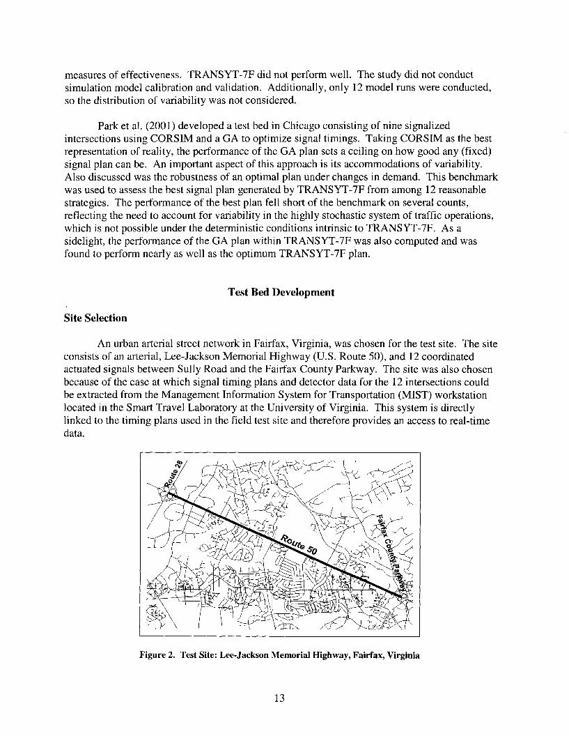
An urban arterial street network in Fairfax, Virginia, was chosen for the test site. The siteconsists of an arterial, Lee-Jackson Memorial Highway (U.S. Route 50), and 12 coordinatedactuated signals between Sully Road and the Fairfax County Parkway. The site was also chosenbecause of the ease at which signal timing plans and detector data for the 12 intersections couldbe extracted from the Management Information System for Transportation (MIST) workstationlocated in the Smart Travel Laboratory at the University of Virginia. This system is directlylinked to the timing plans used in the field test site and therefore provides an access to real-timedata.

Figure 2. Test Site: Lee-Jackson Memorial Highway, Fairfax, Virginia

13

Data Collection

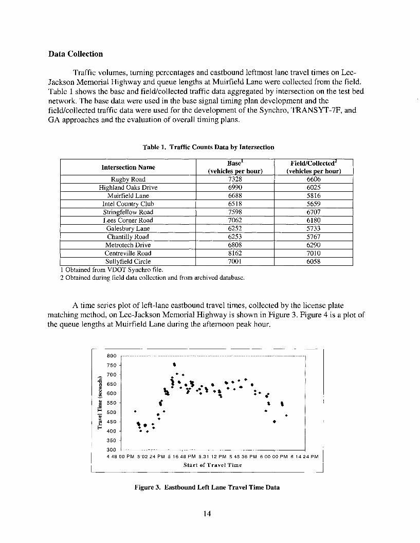
Traffic volumes, turning percentages and eastbound leftmost lane travel times on Lee­Jackson Memorial Highway and queue lengths at Muirfield Lane were collected from the field.Table 1 shows the base and field/collected traffic data aggregated by intersection on the test bednetwork. The base data were used in the base signal timing plan development and thefield/collected traffic data were used for the development of the Synchro, TRANSYT-7F, andGA approaches and the evaluation of overall timing plans.

Table 1. Traffic Counts Data by Intersection

Intersection NameBasel Fieid/Collected2

(vehicles per hour) (vehicles per hour)Rugby Road 7328 6606

Highland Oaks Drive 6990 6025Muirfield Lane 6688 5816

Intel Country Club 6518 5659Stringfellow Road 7598 6707Lees Corner Road 7062 6180Galesbury Lane 6252 5733Chantilly Road 6253 5767

Metrotech Drive 6808 6290Centreville Road 8162 7010Sullyfield Circle 7001 6058

1 Obtained from VDOT Synchro file.2 Obtained during field data collection and from archived database.

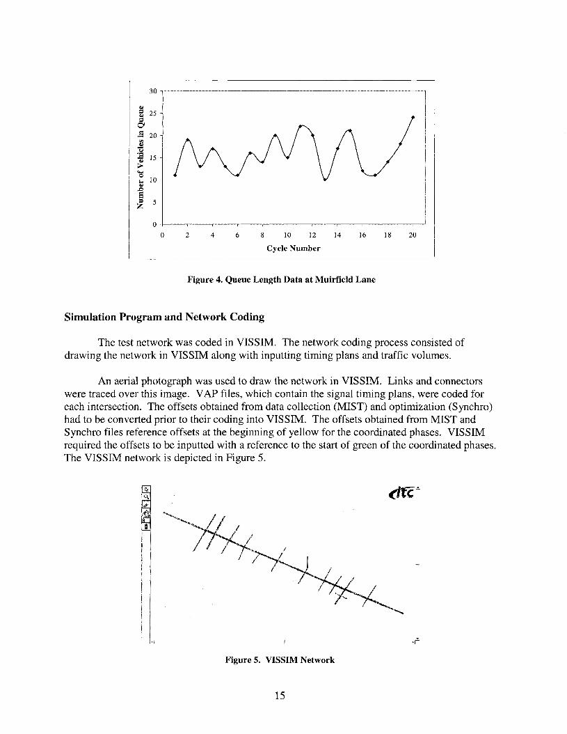
A time series plot of left-lane eastbound travel times, collected by the license platematching method, on Lee-Jackson Memorial Highway is shown in Figure 3. Figure 4 is a plot ofthe queue lengths at Muirfield Lane during the afternoon peak hour.

• ••1~.l • • • ••••t... I •• \ •• ••• •••l& ., ~

(

800

750

-- 700t"-l

"'0 650=0~

600~

~~ 550e

E:: 5001S~

450~l-l~

400

350

• ••• •

••

300 -+------,------r-----....----~--______r---___4

44800PM 5'0224PM 51648PM 5.3112PM 54536PM 60000PM 61424PM

Start of Travel Time

Figure 3. Eastbound Left Lane Travel Time Data

14

30 -----------------------,

QJ

~ 25=o.s 20

r.IJQJ1j

i 15>~o'- 10QJ

,.Qei 5

2018161412108642

O-+----.....----.---r----,----,------r--r---,--.....----.---l

oCycle Number

Figure 4. Queue Length Data at Muirfield Lane

Simulation Program and Network Coding

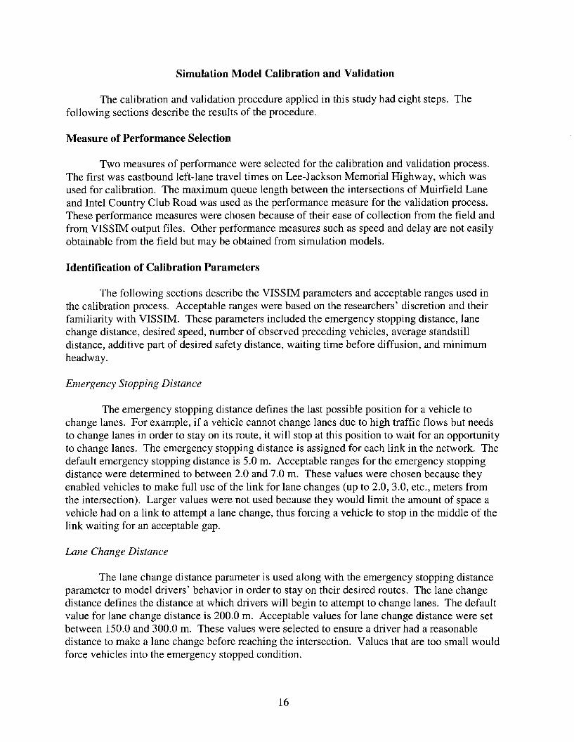
The test network was coded in VISSIM. The network coding process consisted ofdrawing the network in VISSIM along with inputting timing plans and traffic volumes.

An aerial photograph was used to draw the network in VISSIM. Links and connectorswere traced over this image. VAP files, which contain the signal timing plans, were coded foreach intersection. The offsets obtained from data collection (MIST) and optimization (Synchro)had to be converted prior to their coding into VISSIM. The offsets obtained from MIST andSynchro files reference offsets at the beginning of yellow for the coordinated phases. VISSIMrequired the offsets to be inputted with a reference to the start of green of the coordinated phases.The VISSIM network is depicted in Figure 5.

Figure 5. VISSIM Network

15

Simulation Model Calibration and Validation

The calibration and validation procedure applied in this study had eight steps. Thefollowing sections describe the results of the procedure.

Measure of Performance Selection

Two measures of performance were selected for the calibration and validation process.The first was eastbound left-lane travel times on Lee-Jackson Memorial Highway, which wasused for calibration. The maximum queue length between the intersections of Muirfield Laneand Intel Country Club Road was used as the performance measure for the validation process.These performance measures were chosen because of their ease of collection from the field andfrom VISSIM output files. Other performance measures such as speed and delay are not easilyobtainable from the field but may be obtained from simulation models.

Identification of Calibration Parameters

The following sections describe the VISSIM parameters and acceptable ranges used inthe calibration process. Acceptable ranges were based on the researchers' discretion and theirfamiliarity with VISSIM. These parameters included the emergency stopping distance, lanechange distance, desired speed, number of observed preceding vehicles, average standstilldistance, additive part of desired safety distance, waiting time before diffusion, and minimumheadway.

Emergency Stopping Distance

The emergency stopping distance defines the last possible position for a vehicle tochange lanes. For example, if a vehicle cannot change lanes due to high traffic flows but needsto change lanes in order to stay on its route, it will stop at this position to wait for an opportunityto change lanes. The emergency stopping distance is assigned for each link in the network. Thedefault emergency stopping distance is 5.0 m. Acceptable ranges for the emergency stoppingdistance were determined to between 2.0 and 7.0 m. These values were chosen because theyenabled vehicles to make full use of the link for lane changes (up to 2.0, 3.0, etc., meters fromthe intersection). Larger values were not used because they would limit the amount of space avehicle had on a link to attempt a lane change, thus forcing a vehicle to stop in the middle of thelink waiting for an acceptable gap.

Lane Change Distance

The lane change distance parameter is used along with the emergency stopping distanceparameter to model drivers' behavior in order to stay on their desired routes. The lane changedistance defines the distance at which drivers will begin to attempt to change lanes. The defaultvalue for lane change distance is 200.0 m. Acceptable values for lane change distance were setbetween 150.0 and 300.0 m. These values were selected to ensure a driver had a reasonabledistance to make a lane change before reaching the intersection. Values that are too small wouldforce vehicles into the emergency stopped condition.

16

Desired Speed Distribution

The desired speed distribution is an important parameter, having a significant influenceon roadway capacity and achievable travel speeds. The desired speed is the speed a vehicle"desires" to travel if it is not hindered by other vehicles. This is not necessarily the speed thevehicle travels in the simulation. If not hindered by another vehicle, a driver will travel at his orher desired speed (with small oscillations). The more vehicles differ in their desired speed, themore platoons are created. Any driver with a higher desired speed than his or her current travelspeed will check for the opportunity to pass without endangering other vehicles. Minimum andmaximum values can be entered in VISSIM for the desired speed distribution. The speed limiton Lee-Jackson Memorial highway was 45 mph. Acceptable ranges of speed were chosen as setdistributions between 30 and 60 mph, 35 and 55 mph, and 40 and 50 mph. The desired speeddistribution used in this exercise was 35 to 55 mph. This value was chosen based on priorexperience with VISSIM. The 40 to 50 mph desired speed distribution was too tight. Thisdistribution had all vehicles traveling at similar speeds, with little interaction between them. The30 to 60 mph distribution was not chosen because it did not seem reasonable for a vehicle tohave a desired speed of 30 mph.

Number ofObserved Preceding Vehicles

The number of observed preceding vehicles variable affects how well drivers in thenetwork can predict other vehicles' movements and react accordingly. The VISSIM defaultvalue for this parameter is two vehicles. One, two, three, and four vehicles were used in thisstudy.

Average Standstill Distance

Average standstill distance defines the average desired distance between stopped cars andalso between cars and stop lines, signal heads, etc. The default value for average standstilldistance is 2.0 m. Acceptable ranges of values used for this parameter were 1.0 to 3.0 m. Largeror smaller values seemed unreasonable.

Waiting Time Before Diffusion

Waiting time before diffusion defines the maximum amount of time a vehicle can wait atthe emergency stop position waiting for a gap to change lanes in order to stay on its route. Whenthis time is reached, the vehicle is deleted from the network. Sixty seconds is the default value.Other values used in the study were 20 and 40 seconds.

Minimum Headway

VISSIM defines the minimum headway distance as the minimum distance to the vehiclein front that must be available at standstill conditions for a lane change. This parameter couldnot be directly collected from the field. The default value is 0.5 m. The acceptable range used inthe case study was between 0.5 and 7.0 m. The default value seemed too small a distance for

17

drivers to attempt a lane change. It did not seem realistic that a driver would attempt a lanechange given headway of 0.5 m. As a result, larger values were assumed to be more reasonable.

Experimental Design for Calibration

A Latin hypercube experimental design was used for the calibration. Latin hypercubesampling provides an orthogonal array that randomly samples the entire design space brokendown into equal-probability regions. This type of sampling can be looked upon as a stratifiedMonte Carlo sampling where the pair-wise correlations can be minimized to a small value(which is essential for uncorrelated parameter estimates) or else set to a desired value. Latinhypercube sampling is especially useful for exploring the interior of the parameter space and forlimiting the experiment to a fixed (user specified) number of runs. The Latin hypercubetechnique ensures that the entire range of each variable is sampled. A statistical summary of themodel results will produce indices of sensitivity and uncertainty that relate the effects ofheterogeneity of input variables to model predictions. The Latin hypercube design consisted of124 cases using the VISSIM parameters and three values per parameter.

Multiple Runs

Five random seeded runs were conducted in VISSIM for each of the 124 cases, for a totalof 620 runs. The average eastbound left-lane travel time was recorded for each of the 620 runs.The results from the five multiple runs were then averaged to represent each of the 124parameter sets.

Development of a Surface Function

A linear regression model was created in the S-Plus program using the calibrationparameters as independent variables and the eastbound left-lane travel time from VISSIM as thedependant variable, Y. The linear regression model is:

Y =400.88 - 5.10 Xl - 0.68 X2 + 17.80 X3 + 28.63 X4 + 1.77Xs + 30.20 X6

where,

Y = eastbound left-lane travel time (sec)Xl = emergency stopping distance (m), t value: -2.31, p value: < 0.0212X2 =lane change distance (meters), t value: -9.15, p value: < 0.0001X3 =number of observed preceding vehicles, t value: 3.69, p value: 0.0002X4 =standstill distance (m), t value: 5.93, p value: < 0.0001Xs =waiting time before diffusion (sec), t value: 7.32, p value: < 0.0001X6 = minimum headway (m), t value: 11.37, P value: < 0.0001

18

Candidate Parameter Sets

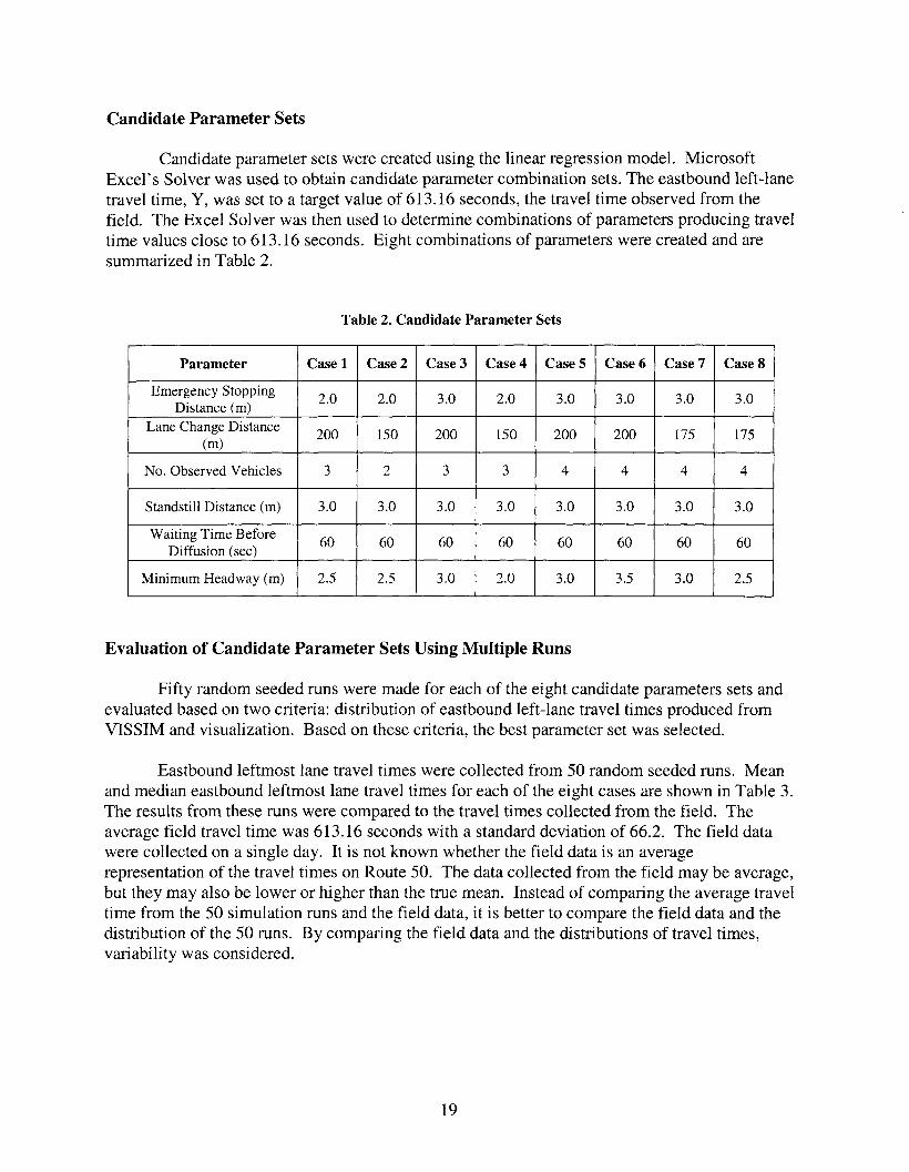
Candidate parameter sets were created using the linear regression model. MicrosoftExcel's Solver was used to obtain candidate parameter combination sets. The eastbound left-lanetravel time, Y, was set to a target value of 613.16 seconds, the travel time observed from thefield. The Excel Solver was then used to determine combinations of parameters producing traveltime values close to 613.16 seconds. Eight combinations of parameters were created and aresummarized in Table 2.

Table 2. Candidate Parameter Sets

Parameter Case 1 Case 2 Case 3 Case 4 CaseS Case 6 Case 7 CaseS

Emergency Stopping 2.0 2.0 3.0 2.0 3.0 3.0 3.0 3.0Distance (m)

Lane Change Distance 200 150 200 150 200 200 175 175(m)

No. Observed Vehicles 3 2 3 3 4 4 4 4

Standstill Distance (m) 3.0 3.0 3.0 3.0 3.0 3.0 3.0 3.0

Waiting Time Before 60 60 60 60 60 60 60 60Diffusion (sec)

Minimum Headway (m) 2.5 2.5 3.0 2.0 3.0 3.5 3.0 2.5

Evaluation of Candidate Parameter Sets Using Multiple Runs

Fifty random seeded runs were made for each of the eight candidate parameters sets andevaluated based on two criteria: distribution of eastbound left-lane travel times produced fromVISSIM and visualization. Based on these criteria, the best parameter set was selected.

Eastbound leftmost lane travel times were collected from 50 random seeded runs. Meanand median eastbound leftmost lane travel times for each of the eight cases are shown in Table 3.The results from these runs were compared to the travel times collected from the field. Theaverage field travel time was 613.16 seconds with a standard deviation of 66.2. The field datawere collected on a single day. It is not known whether the field data is an averagerepresentation of the travel times on Route 50. The data collected from the field may be average,but they may also be lower or higher than the true mean. Instead of comparing the average traveltime from the 50 simulation runs and the field data, it is better to compare the field data and thedistribution of the 50 runs. By comparing the field data and the distributions of travel times,variability was considered.

19

Table 3. Evaluation of Candidate Parameter Sets: Leftmost Lane Travel Time

Case Mean (sec) Median (sec)Standard Percentile Field t testDeviation Value (p value)

1 449.6 439.5 57.5 100% 0.002 603.2 596.1 88.3 54% 0.423 473.7 465.3 64.3 98% 0.264 688.9 681.9 115.5 24% 0.405 467.9 455.9 59.3 98% 0.046 519.0 508.7 70.7 92% 0.857 523.2 523.2 70.6 90% 0.728 485.3 476.6 63.7 98% 0.00

The t test was used to determine if the travel times produced by VISSIM werestatistically equal to the field travel times. In order to perform a t test, it was necessary to selectthe travel time results from a single VISSIM run and compare these travel times to thoseobserved in the field. The VISSIM results that produced mean travel times closest to thoseobserved from the field were selected for t test comparisons. Table 3 shows the results of the ttests. The percentile field values in the table show the percentage of runs, from the 50 multipleruns, which were less than the VISSIM results used for the t test.

Because of the variability in VISSIM runs and results, the t test is extremely sensitive. Itis likely that in most cases, the t test would indicate that the field distribution of left-most lanetravel time is statistically different from simulation-based results based on this variability.However, for a few runs close to the observed field travel times, the t test may conclude that thetwo are statistically the same.

The importance of visualization when using microscopic simulation models cannot beoveremphasized. The purpose of the microscopic simulation model is to represent the fieldconditions as closely as possible. A model cannot be deemed calibrated if the animations are notrealistic. For example, a parameter set may be statistically acceptable but the animations maynot be realistic. Then, the model is not acceptable. Animations from the 50 multiple runs wereviewed in order to identify at which percentile animations were not acceptable. An example ofan unacceptable animation is depicted in Figure 6.

20

Figure 6. Example of an Unacceptable Animation in VISSIM

In this VISSIM screenshot, unrealistic animations occur in the westbound direction thatwere not observed in the field. Vehicles in the figure are attempting to make lane changes at thestop bar. Vehicles in the leftmost lane are trying to make right turns, and vehicles in therightmost lane are attempting to make left turns. The vehicles were not able to make theirdesired lane change within the link and therefore are at an emergency stopped position. Theywill stay at that position, blocking other vehicles, until they are able to change lanes or they arekicked out of the system (due to waiting time before diffusion). Regardless of the travel timesproduced from an animation like this, this parameter set cannot be chosen because its visual doesnot represent the real world.

Animations of each case were viewed in order to determine whether the animations wererealistic or unrealistic. Each case was viewed at several travel time percentiles in order todetermine if the animations were realistic or not. It was found that cases 2 and 4 were notacceptable.

Parameter set 7 was chosen as the best parameter set based on its travel time distribution(Figure 7), statistical tests, and animations. Parameter sets 2 and 4 were eliminated because theiranimations were unrealistic. Parameter sets 1, 3, 5, and 8 were eliminated based on their t testresults. Parameter 7 produced travel times closest to those from the field. Parameter sets 6 and 7produced similar results, but parameter set 7 was chosen because its animations were morerealistic.

21

25 --.--.............------------............----------,

20 Field: 613.2 seconds

800700600500400

O---......--=::=~"------,-------r-----r-.-- .....---.

300

5

>-g 15CD::::JC'"! 10LL

Travel Time (seconds)

Figure 7. Eastbound Left Lane Travel Time Distribution of Parameter Set 7

Validation with New Field Data

The eastbound maximum queue length between the intersections of Muirfield Lane andIntel County Club Road was used for validation of parameter set 7. The maximum queue lengthdata were collected on a different day, and the input volumes used for the validation processwere untried. The maximum queue length observed in the field was compared to the distributionof 100 runs in VISSIM. The field maximum queue length was about the top 90 percent of thesimulated distribution, as shown in Figure 8.

40353025

Field: 24 vehicles

2015105

10

5

O--+----.,.-------..-:;~-...,.----..,..---...,...-........~......---t-t----t

o

35 -------- -- - - - -......-."

30

25~ui 20::::Jg 15~

LL

Maximum Queue (Vehicles)

Figure 8. Maximum Queue Length Histogram of Parameter Set 7

22

Signal Timing Plan Optimization and Evaluation

Signal Timing Plan Optimization

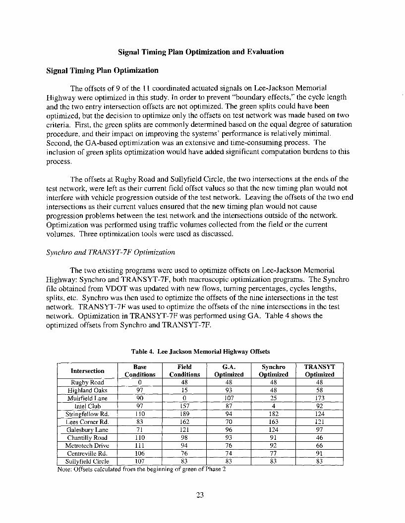
The offsets of 9 of the 11 coordinated actuated signals on Lee-Jackson MemorialHighway were optimized in this study. In order to prevent "boundary effects," the cycle lengthand the two entry intersection offsets are not optimized. The green splits could have beenoptimized, but the decision to optimize only the offsets on test network was made based on twocriteria. First, the green splits are commonly determined based on the equal degree of saturationprocedure, and their impact on improving the systems' performance is relatively minimal.Second, the GA-based optimization was an extensive and time-consuming process. Theinclusion of green splits optimization would have added significant computation burdens to thisprocess.

The offsets at Rugby Road and Sullyfield Circle, the two intersections at the ends of thetest network, were left as their current field offset values so that the new timing plan would notinterfere with vehicle progression outside of the test network. Leaving the offsets of the two endintersections as their current values ensured that the new timing plan would not causeprogression problems between the test network and the intersections outside of the network.Optimization was performed using traffic volumes collected from the field or the currentvolumes. Three optimization tools were used as discussed.

Synchro and TRANSYT-7F Optimization

The two existing programs were used to optimize offsets on Lee-Jackson MemorialHighway: Synchro and TRANSYT-7F, both macroscopic optimization programs. The Synchrofile obtained from VDOT was updated with new flows, turning percentages, cycles lengths,splits, etc. Synchro was then used to optimize the offsets of the nine intersections in the testnetwork. TRANSYT-7F was used to optimize the offsets of the nine intersections in the testnetwork. Optimization in TRANSYT-7F was performed using GA. Table 4 shows theoptimized offsets from Synchro and TRANSYT-7F.

Table 4. Lee Jackson Memorial Highway Offsets

IntersectionBase Field G.A. Synchro TRANSYT

Conditions Conditions Optimized Optimized OptimizedRugby Road 0 48 48 48 48

Highland Oaks 97 15 93 48 58Muirfield Lane 90 0 107 25 173

Intel Club 97 157 87 4 92Stringfellow Rd. 110 189 94 182 124Lees Corner Rd. 83 162 70 163 121Galesbury Lane 71 121 96 124 97Chantilly Road 110 98 93 91 46

Metrotech Drive 111 94 76 92 66Centreville Rd. 106 76 74 77 91

Sullyfield Circle 107 83 83 83 83Note: Offsets calculated from the beginning of green of Phase 2

23

Genetic Algorithm Optimization

A GA was linked to the calibrated VISSIM model of Lee-Jackson Memorial Highway tooptimize offsets. A weighted average of travel times, eastbound and westbound, was used as thefitness value for the GA. Offset optimization was performed twice using the GA. The firstapproach used four VISSIM runs per timing plan to assign fitness values to a set of offsets.Figure 9 shows the convergence of the GA. As the number of generations increase, the weightedaverage travel time approaches the minimum travel time. The final fitness value produced aweighted average travel time of 538.8 seconds.

The second GA optimization used eight VISSIM runs per set of offsets to determine afitness value. This approach was considered because of the variability in VISSIM travel times.Because of the variability in travel times, using four runs to assign fitness values may not beadequate. This small sample could quite easily be at either extreme of the distribution, thusassigning a fitness value that is either too large or too small. Naturally increasing the number ofruns would help but is time-consuming when using the GA. Figure 10 shows the convergence ofthe GA using eight runs to determine fitness values. The minimum average travel time was528.8 seconds, 10 seconds less than when four runs were used to determine fitness values. Table4 shows the optimized offsets from the GA optimization.

~ 650

~! 600

CDEi= 550CD>co~ 500

- average - minimum

3 5 7 9 11 13 15 17 19 21 23 25

Generation

Figure 9. GA Travel Time Convergence (4 VISSIM runs per timing plan)

24

:2 650

~! 600

~i= 550

~ca...I- 500

-average -minimum

3 5 7 9 11 13 15 17 19 21 23 25

Generation

Figure 10. GA Travel Time Convergence (8 VISSIM runs per timing plan)

Signal Timing Plan Evaluation

Five timing plans were under evaluation in this study: (1) the base timing plan, (2) thefield timing plan, (3) the GA optimized timing plan, (4) the Synchro optimized timing plan, and(5) the TRANSYT-7F optimized timing plan. Each plan was evaluated using VISSIM. Theoffset values for the five timing plans are shown in Table 4. The base timing plan was takenfrom VDOT's Synchro file. This timing plan was used by VDOT in the field prior to its currenttiming plan. The timing plan has a cycle length of 180 seconds. VDOT recently implementedits current timing plan, denoted as the field timing plan in this report. The cycle length of thistiming plan is 190 seconds and it contains different green splits than the base timing plan. Thethree optimized timing plans have the same cycle length and green splits as the field timing planbut contain new offset values.

Two measures of performance were used to evaluate the five timing plans. The first wastravel time on Lee-Jackson Memorial Highway. The weighted average of travel times forwestbound and eastbound traffic was used. Travel time collection points were set at thebeginning and end of the test network at the intersections of Route 50 and Sully Road and theFairfax County Parkway. Travel time was collected from VISSIM through *.rsr files for eachrun. The *.rsr files contain every completed travel time measurement event in chronologicalorder. Because multiple runs were conducted, resulting in 100 *.rsr files, a Rexx program wascreated to ease the computational burden. The Rexx program calculated the mean and standarddeviation for each of the 100 runs and outputted a summary file containing eastbound andwestbound throughputs, travel times, and standard deviations.

The second performance measure was the total system delay. Unfortunately, VISSIMdoes not calculate total system delay as one of its outputs. In order to find the total system delay,multiple delay collection points were created. Delay segments are similar to travel timecollection points. Two points on the test network are chosen, and delay is determined as thedifference between actual travel time and the travel time if the vehicle was driving unobstructedat its desired speed. In order to determine the total system delay, delay segments were set up for

25

every possible combination of vehicle inputs and outputs in the network. For example, for everyplace a vehicle entered the network, a delay segment had to be created for every combination ofwhere the vehicle might exit the network. The total system delay was determined as a weightedaverage of all of the delays. The total system delay was obtained through *.vlz files fromVISSIM.

VDOT's former and current timing plans were evaluated in VISSIM to determine if theirnew timing plan (field) performed better than their former timing plan (base). The mean traveltime on Lee-Jackson Memorial Highway decreased from 625.9 to 518.9 seconds, a 17.1 %reduction. The improvement in travel times can better be seen using the histogram depicted inFigure 11. The field histogram is shifted to the left, or toward shorter travel times. The fieldtiming plan also produces a tighter distribution than the base timing plan. The tightness of thedistribution means that the majority of the VISSIM runs produced travel times close to the mean.The base timing plan shows larger variations in travel times.

1000900800700600500400

20

10

O_._--IIII--_&r--......- .....-c.---,--..III!::::===IIII=-__j..-:=8--__--III-_III--_._

300

~(J

~ 40:::sg 30...u.

70 --,---.............----...........................-------------------.

60

50

Travel Time (seconds)

1-.-Base Timing Plan --- Field Timing Plan I

Figure 11. Base and Field: Weighted Average Travel Time Histograms

The total system delay was also improved. The mean total system delay was decreasedfrom 248.0 seconds per vehicle with the base timing plan to 157.2 seconds with the field timingplan, a 36.6% reduction. Evaluation of the two VDOT timing plans shows considerableimprovement. Travel times and total system delay are improved with the use of the currenttiming plan.

Although the current VDOT timing plan outperformed its predecessor, optimization toolswere evaluated to determine if they could improve upon the current timing plan. The processused to evaluate the three optimized timing plans was the same as the one used to evaluate thetwo VDOT timing plans. Travel times on Lee-Jackson Memorial Highway and total systemdelay were used for evaluation. The three optimized timing plans were compared to each other

26

as well as to the field timing plan in order to determine which of the four timing plans workedbest.

Table 5 shows the weighted average of travel times for 100 runs in VISSIM. As seen inthe table, it appears that there is no significant improvement of the mean field travel time of518.9 seconds. Figure 12 shows the travel time histograms. The field, Synchro optimized, andGA optimized timing plans are strikingly similar. Their mean travel times are also similar. TheTRANSYT-7F optimized timing plan is shifted to the right and shows a much larger mean traveltime (555.6 seconds) than the other three timing plans.

Table 5. VISSIM Multiple Run Travel Time Results

Timing PlanMean Travel Median Travel Standard

Time (sec) Time (sec) DeviationBase 625.9 621.2 136.9Field 518.9 512.5 72.7

Synchro 512.3 511.0 71.9

TRANSYT 555.6 549.7 78.9

GA 520.1 515.4 67.6

1000900800700600500400

70 --r---..............-----.............---.............- .............--................-..........................- .............---.,

60

~ 50(,)

; 40::Jg- 30...u.. 20

10

o ..._---f'.Im----«l__

300

Travel Time (seconds)

--- Field Timing Plan Synchro Optimized

, TRANSYT-7F Optimized --'-G.A. Optimized

Figure 12. Optimized Timing Plans: Weighted Average Travel Time Histograms

Because the field, Synchro optimized, and GA optimized timing plans gave similar traveltime results, a t test was conducted to test if the mean travel times of one timing plan were equalto the mean travel time of another timing plan. Null and alternative hypotheses were set for eachcombination. For each case, the null hypothesis was that the two data sets were equal. Thealternative hypothesis was that the data sets were unequal. P values were determined for eachcase. The p value provides an objective measure of the strength of evidence the data supply in

27

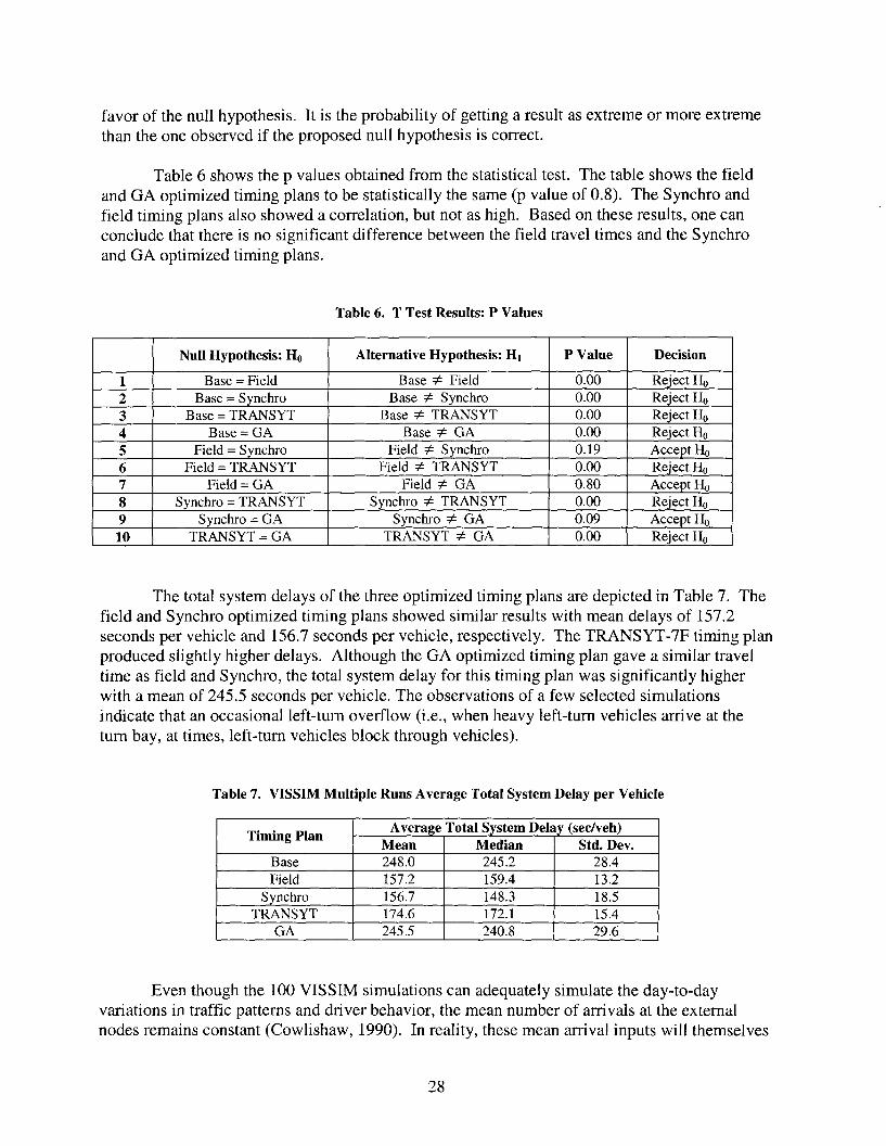
favor of the null hypothesis. It is the probability of getting a result as extreme or more extremethan the one observed if the proposed null hypothesis is correct.

Table 6 shows the p values obtained from the statistical test. The table shows the fieldand GA optimized timing plans to be statistically the same (p value of 0.8). The Synchro andfield timing plans also showed a correlation, but not as high. Based on these results, one canconclude that there is no significant difference between the field travel times and the Synchroand GA optimized timing plans.

Table 6. T Test Results: P Values

Null Hypothesis: Ho Alternative Hypothesis: HI P Value Decision

1 Base = Field Base "* Field 0.00 Reject Ho2 Base = Synchro Base "* Synchro 0.00 Reject Ho3 Base = TRANSYT Base"* TRANSYT 0.00 Reject Ho4 Base = GA Base"* GA 0.00 Reject Ho5 Field = Synchro Field "* Synchro 0.19 Accept Ho6 Field = TRANSYT Field "* TRANSYT 0.00 Reject Ho7 Field = GA Field"* GA 0.80 Accept Ho8 Synchro = TRANSYT Synchro "* TRANSYT 0.00 Reject Ho9 Synchro = GA Synchro"* GA 0.09 Accept Ho10 TRANSYT=GA TRANSYT"* GA 0.00 Reject Ho

The total system delays of the three optimized timing plans are depicted in Table 7. Thefield and Synchro optimized timing plans showed similar results with mean delays of 157.2seconds per vehicle and 156.7 seconds per vehicle, respectively. The TRANSYT-7F timing planproduced slightly higher delays. Although the GA optimized timing plan gave a similar traveltime as field and Synchro, the total system delay for this timing plan was significantly higherwith a mean of 245.5 seconds per vehicle. The observations of a few selected simulationsindicate that an occasional left-tum overflow (i.e., when heavy left-tum vehicles arrive at thetum bay, at times, left-tum vehicles block through vehicles).

Table 7. VISSIM Multiple Runs Average Total System Delay per Vehicle

Timing PlanAverage Total System Delay (sec/veh)

Mean Median Std. Dev.Base 248.0 245.2 28.4Field 157.2 159.4 13.2

Synchro 156.7 148.3 18.5TRANSYT 174.6 172.1 15.4

GA 245.5 240.8 29.6

Even though the 100 VISSIM simulations can adequately simulate the day-to-dayvariations in traffic patterns and driver behavior, the mean number of arrivals at the externalnodes remains constant (Cowlishaw, 1990). In reality, these mean arrival inputs will themselves

28

change over time. Moreover, the estimates of these mean rates are based on traffic countscollected by manual observers and are subject to considerable error. Therefore, the responses ofthe timing plans to changes in these mean rates were evaluated.

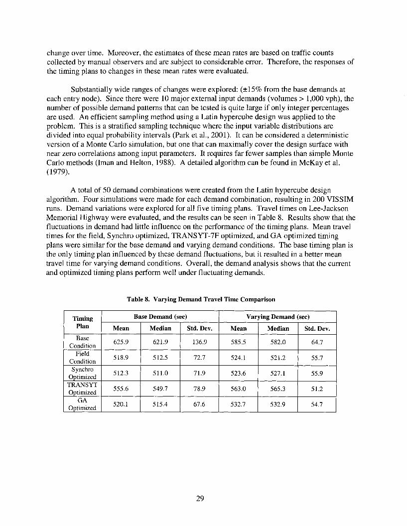
Substantially wide ranges of changes were explored: (±15% from the base demands ateach entry node). Since there were 10 major external input demands (volumes> 1,000 vph), thenumber of possible demand patterns that can be tested is quite large if only integer percentagesare used. An efficient sampling method using a Latin hypercube design was applied to theproblem. This is a stratified sampling technique where the input variable distributions aredivided into equal probability intervals (Park et aI., 2001). It can be considered a detenninisticversion of a Monte Carlo simulation, but one that can maximally cover the design surface withnear zero correlations among input parameters. It requires far fewer samples than simple MonteCarlo methods (Iman and Helton, 1988). A detailed algorithm can be found in McKay et aI.(1979).

A total of 50 demand combinations were created from the Latin hypercube designalgorithm. Four simulations were made for each demand combination, resulting in 200 VISSIMruns. Demand variations were explored for all five timing plans. Travel times on Lee-JacksonMemorial Highway were evaluated, and the results can be seen in Table 8. Results show that thefluctuations in demand had little influence on the perfonnance of the timing plans. Mean traveltimes for the field, Synchro optimized, TRANSYT-7F optimized, and GA optimized timingplans were similar for the base demand and varying demand conditions. The base timing plan isthe only timing plan influenced by these demand fluctuations, but it resulted in a better meantravel time for varying demand conditions. Overall, the demand analysis shows that the currentand optimized timing plans perfonn well under fluctuating demands.

Table 8. Varying Demand Travel Time Comparison

Timing Base Demand (sec) Varying Demand (sec)

Plan Mean Median Std. Dev. Mean Median Std. Dev.

Base625.9 621.9 136.9 585.5 582.0 64.7Condition

Field518.9 512.5 72.7 524.1 521.2 55.7

ConditionSynchro

512.3 511.0 71.9 523.6 527.1 55.9OptimizedTRANSYT

555.6 549.7 78.9 563.0 565.3 51.2OptimizedGA

520.1 515.4 67.6 532.7 532.9 54.7Optimized

29

CONCLUSIONS

Statistical testing and visualization are the most critical aspects of the simulation modelcalibration and validation. The statistical testing dealt with when to claim the calibrated model is"equal" to the field data, and the visualization dealt with if the animation looks "real" as seen inthe field.

The statistical testing is due to the variability in simulation runs. All multiple runs werenot statistically equal to the field distribution. In other words, the simulation output passed thestatistical test at different percentiles for each parameter set. Given that the field data are justone realization of an infinite stochastic process, this seems natural. Thus, individual runs maynot be applicable for statistical testing. Instead, the simulation results that are most close to thefield data can be used. If the data pass this test, it ensures that the field data were represented atleast once in the simulation model. In addition, the percentile of field average value at thedistribution of the simulation output can be used to determine how the simulation represents fieldcondition.

The importance of visualization cannot be overstated. Although obtaining measures ofperformance from the simulation close to those observed in the field is important, if theanimations are not realistic, the model should not be considered calibrated. The purpose ofmicroscopic simulation models is to represent the real world as closely as possible. Simulationmodels that generate behavior not exhibited in the field are unrealistic. Thus, parameter setsproducing unrealistic simulations should not be considered.

Evaluation of timing plans revealed a significant benefit of using the current VDOTtiming plan rather than the one previously used. The new timing plan resulted in a 17.1%reduction in travel time on Lee-Jackson Memorial Highway and a 36.6% reduction in totalsystem delay. It is therefore concluded that VDOT's current methodology for setting timingplans works well in improving performance.

This 17.1% travel time saving translates to 53,054 hours of time saved per year for allvehicles traveling on Lee-Jackson Memorial Highway in the afternoon peak hour. The delayreduction saves a combined 100,061 hours per year for afternoon peak hour for all vehicles in thesystem. Delay savings were calculated by taking the difference of average delay per vehicle forthe base and field conditions. This difference, which was the time savings for the weekdayafternoon peak hour, was multiplied by the total number of vehicles in the system. The resultwas multiplied by the number of weekdays in a year to determine the total annual cost savings.Assuming time savings can be given a monetary value, the user delay savings is roughly$515,317. This value is based on the assumption that each hour of time saved is equivalent toVirginia's minimum wage of $5.15 per hour.

It should be noted that the time savings and benefits stated in this report are based on thedemand conditions collected from the field and used in the simulation model. Even thoughdifferent demand conditions may result in different time savings and delay reductions, it isexpected that the implementation of the new timing plan will result in time savings and delayreductions.

30

The timing plans from three optimization tools were also evaluated in VISSIM todetermine if the performance of the current timing plan on Lee-Jackson Memorial Highwaycould be improved upon. The GA, Synchro, and TRANSYT-7F optimized timing plans did notyield significant benefits over those for VDOT's current timing plan.

RECOMMENDATIONS

1. Evaluation of the test site shows that the current VDOT signal optimization proceduresignificantly improves the performance of network operations. Thus, it is recommended thatVDOT continue to use its procedure for developing new timing plans.

2. Although the current (field) timing plan, which was updated in April 2001, performs well, itis recommended that (1) VDOT evaluate its existing timing plan regularly in an effort tokeep the plan up to date, and (2) VTRC conduct a follow-up study to identify when thecurrent signal timing plan should be re-optimized. The timing for this research can bedetermined by monitoring the trend of traffic patterns, including the changes of trafficdemand, turning percentages, vehicle mix, etc., and conducting a cost-benefit analysisbetween the existing and new timing plans.

3. As this study substantiates that traffic signal optimization is an effective way of improvingurban network mobility, it is recommended that VDOT allocate more time and effort towardupdating traffic signal timing plans in Northern Virginia as well as the rest of the state.

4. In this study, the proposed simulation calibration and validation procedure used only a singleday of field data and two measures of performance. It is recommended that VTRC conductfurther research that uses multiple days of field data in order to account for variability andvalidate the proposed procedure with other test networks. Such research is underway.

REFERENCES

Beasley, D., D. R. Bull, and R. R. Martin. An Overview of Genetic Algorithms: Part I,Fundamentals. University Computing, Vol. 15, No.2, 1993, pp. 58-69.

Cheu, R., X. Jin, K. Ng, Y. Ng, and D. Srinivasan. Calibration of FRESIM for SingaporeExpressway Using Genetic Algorithm. Journal of Transportation Engineering,November/December 1998.

Cowlishaw, M. F. The REXX Language, Second Edition. Prentice-Hall, Englewood Cliffs, NJ,1990.

CORSIM User's Manual. FHWA, U.S. Department of Transportation, Office of Safety andTraffic Operations, McLean, VA, 1997.

31

Goldberg, D.E. Genetic Algorithms in Search, Optimization, and Machine Learning. Addison­Wesley Publishing Co., Inc., Reading, MA, 1989.

Hellinga, B. R. Requirements for the Calibration of Traffic Simulation Models. Department ofCivil Engineering, University of Waterloo. http://www.civil.uwaterloo.ca/b.PDF. Lastviewed March 2002.

Iman, R. L., and J. Helton. An Investigation of Uncertainty and Sensitivity Analysis Techniquesfor Computer Models. Risk Analysis, Vol. 4, 1988, pp. 71-90.

Lee, D., and X. Yang. Parameter Optimization for PARAMICS Using a Genetic Algorithm.Paper presented at the 6th International Conference on Applications on AdvancedTechnologies in Transportation Engineering, June 2000, Singapore.

McKay, M. D., R. J. Beckman, and W. J. Conover, A Comparison of Three Methods forSelecting Values of Input Variables in the Analysis of Output from a Computer Code.Technometrics, Vol. 21, 1979, pp. 239-245.

Milam, R. T. Recommended Guidelines for the Calibration and Validation of Traffic SimulationModels. Fehr & Peers Associates, Inc.http://www.fehrandpeers.comlpublications/traff simulation m.html. Last viewed March2002.

Paracha, J. Software Choices for Intersection Signals. Better Roads. Vol. 69, No.9. September1999, pp. 25-27.

Park, B., C. J. Messer, and T. Urbanik II. Traffic Signal Optimization Program for OversaturatedConditions: A Genetic Algorithm Approach. Transportation Research Record 1683,TRB, National Research Council, Washington, DC, 1999, pp. 133-142.

Park, B., N. M. Rouphail, and J. Sacks. Assessment of A Stochastic Signal Optimization MethodUsing Microsimulation. Transportation Research Record 1748, TRB, National ResearchCouncil, Washington, DC, 2001, pp. 40-45.

Rouphail, N. M., B. Park, and J. Sacks. Direct Signal Timing Optimization: StrategyDevelopment and Results. In XI Pan American Conference in Traffic and TransportationEngineering, Brazil, November 19-23,2000.

Sacks, J., N. Rouphail, B. Park, and P. Thakuriah. Statistically Based Validation of ComputerSimulation Models in Traffic Operations and Management. Journal ofTransportationand Statistics, 2003.

Synchro 4.0 User's Guide, Trafficware, Albany, CA, 1999.

TRANSYT-7F's User's Manual. Transportation Research Center, University of Florida,Gainesville, FL., March 1998.

32

VISSIM Version 3.6 Manual. PTV Planug Transport Verkehr AG. Innovative TransportationConcepts LLC, Karlsruhe, Germany, December 2001.

Yang, X. K. Comparison among Computer Packages in Providing Timing Plans for IowaArterial in Lawrence Kansas. Journal o/Transportation Engineering, Vol. 127, No.4,July/August 2001.

33