Evaluation of the WRF model based on observations

made by controlled meteorological balloons

in the atmospheric boundary layer of Svalbard

Author:Marina Lara Dutsch

Supervisor:Lars Robert Hole

September 7, 2012

Abstract

In the period of 5 May 2011 to 12 May 2011, five controlled meteorological balloons werelaunched from Ny Alesund on Svalbard. They measured vertical profiles over the coastalarea in the vicinity of Ny Alesund and over sea ice to the east of Svalbard. Togetherwith timeseries measured by three meteorological research stations, the profiles measuredby the balloons were used to evaluate the performance of the Weather Research andForecasting model and in particular of three different boundary layer schemes appliedin the model. The largest errors were found in the profiles over sea ice, where the modelunderestimated potential temperature and overestimated wind speed. Furthermore, themodel showed difficulties in capturing temperature inversions and low level jets. TheQuasi-Normal Scale Elimination scheme yielded the lowest errors and highest correlationfor the timeseries, while the Yonsei University scheme achieved the best results for thevertical profiles.

I

Contents

1 Introduction 1

2 The numerical model 42.1 Sea Ice . . . . . . . . . . . . . . . . . . . . . . . . . . . . . . . . . . . . . . 6

3 The balloon flights 73.1 Comparison with radiosoundings . . . . . . . . . . . . . . . . . . . . . . . 9

4 Results 154.1 The synoptical situation . . . . . . . . . . . . . . . . . . . . . . . . . . . . 154.2 Model run 1: Coastal area . . . . . . . . . . . . . . . . . . . . . . . . . . . 194.3 Model run 2: Sea ice . . . . . . . . . . . . . . . . . . . . . . . . . . . . . . 274.4 Timeseries . . . . . . . . . . . . . . . . . . . . . . . . . . . . . . . . . . . . 31

4.4.1 Wind roses . . . . . . . . . . . . . . . . . . . . . . . . . . . . . . . 32

5 Discussion 405.1 Wind . . . . . . . . . . . . . . . . . . . . . . . . . . . . . . . . . . . . . . . 405.2 Temperature . . . . . . . . . . . . . . . . . . . . . . . . . . . . . . . . . . 405.3 Relative humidity . . . . . . . . . . . . . . . . . . . . . . . . . . . . . . . . 415.4 Parameterisation schemes . . . . . . . . . . . . . . . . . . . . . . . . . . . 41

6 Future work 42

7 Acknowledgements 43

References 44

III

1 Introduction

At high latitudes, global warming leads to surface temperatures increasing by a ratemuch higher than at low latitudes (3◦C to 10◦C at the North Pole compared to 2◦C to4◦C in the tropics for a doubling of CO2 (Lu and Cai, 2010)), a phenomenon which isknown as polar amplification (PA). PA indicates a higher climate sensitivity of polar re-gions due to mechanisms such as the surface albedo feedback, increased poleward energytransport, water vapour feedback, cloud processes and damping of outgoing longwaveradiation by thermal inversions, a.o. (Bintanja et al., 2011). It makes polar regions playa critical role in future climate projections.

However, the range of warming at high latitudes simulated in global climate mod-els (GCMs) in response to increasing greenhouse gas concentrations is large (Houghtonet al., 2001). The large spread can partly be explained by the lack of observationaldata for polar regions, which would be required to initialise and validate the model, aswell as by the fact that the parameterisations applied in GCMs are often adapted toand validated against lower latitudes and might not necessarily be applicable to highlatitudes. Furthermore, polar regions provide a rather complex area and therefore achallenge to numerical models: Advection of sea ice and thermodynamic ice formation,growth and melt can lead to high temporal and spatial variations in surface conditions.While the surface temperature of open water areas is practically at the freezing point ofwater (-1.8◦C), the surface temperature of thick snow covered sea ice can be less than-40◦C. Hence, the turbulent surface fluxes can vary by up to two orders of magnitude(Kilpelainen et al., 2011). In addition, the stratification of the atmospheric boundarylayer (ABL) over sea ice is usually strongly stable during winter, and weakly stable toneutral during summer (Persson et al., 2002). Strong stable stratification implies thateffects of flows over small-scale topography, such as channelling, katabatic flows andmountain waves, are comparable to effects of flows over much higher topography duringunstable stratification. Modelling of these effects would then require a much higher hor-izontal and vertical resolution (than currently available for GCMs).

To improve the understanding and modelling of the important physical processes tak-ing place in polar regions, Regional Climate Models (RCMs) can help. They typicallyhave a higher resolution and hence a better treatment of topography, land-sea mask andsmall-scale physical processes than GCMs. Moreover, the physics of the model can beoptimised for polar conditions. Rinke et al. (2006) compared simulations of eight differ-ent RCMs over the Western Arctic for the period September 1997 - September 1998 (theyear of the Surface Heat Budget of the Arctic Ocean (SHEBA) campaign) to EuropeanCenter for Medium-Range Weather Forecasts (ECMWF) analyses. They found that themodel ensemble mean in general agrees well with the ECMWF analyses. Yet, there wasa large across-model scatter, especially for the 2m temperature over land, the surface

1

radiation fluxes and cloud cover, and mainly in the lowest model levels, which indicatesa still high uncertainty in current Arctic RCM simulations.

In this study, we will verify the Weather Research and Forecasting (WRF) mesoscalemodel against profiles measured by controlled meteorological (CMET) balloons launchedin May 2011 from Ny Alesund on Svalbard. CMET balloons are unique in that theiraltitude can be controlled by operators on the ground via a satellite link. It is thereforepossible to take vertical soundings at any time during the balloon flight. In addition,since no helium is released during the flight, the balloons are able to fly long and far,which gives us the opportunity to investigate areas far away from research bases. CMETballoons were developed at the Smith College, USA, and have been previously used by,e.g., Riddle et al. (2006), Voss et al. (2010) and Mentzoni (2011). Voss et al. (2010)investigated the evolving vertical structure of the polluted Mexico City Area outflow bymaking repeated balloon profile measurements of temperature, humidity and wind in theadvecting outflow. Riddle et al. (2006) and Mentzoni (2011) used the CMET balloonsas a tool to verify atmospheric trajectory models - namely FlexTra (Stohl et al., 1995)and FlexPart (Stohl et al., 1998) - in the United States and in the Arctic, respectively.

Due to the rather harsh conditions, which make it difficult to carry out field cam-paigns in polar regions, only few studies have been conducted that compare observa-tions (in particular balloon measurements) to a mesoscale model in the Arctic. WRFhas previously been evaluated against measurements from weather stations on Green-land, Svalbard and the Arctic Ocean. E.g., Hines and Bromwich (2008) validated apolar optimised version of WRF (Polar WRF) against measurements from automaticweather stations (AWS) on the Greenland ice sheet in June 2001 and December 2002.Bromwich et al. (2009) used the detailed measurements gained during the SHEBA pro-gram in 1997 - 1998 to evaluate the same model (Polar WRF) over the Arctic Ocean.Kilpelainen et al. (2011) compared model results from the standard WRF model totower observations and radiosoundings in three Svalbard fjords in winter and spring2008. Livik (2011) evaluated WRF against measurements from AWS placed at severallocations along Kongsfjorden, Svalbard, in spring 2010. Makiranta et al. (2011) com-pared WRF to mast measurements made in Wahlenbergfjorden, Svalbard, in May 2006and April 2007, and Kilpelainen et al. (2012) compared both polar and standard WRFto tethered balloon soundings and mast observations taken in March and April 2009.In addition, Mayer et al. (2012a) and Mayer et al. (2012b) used the recently developedsmall unmanned meteorological observer (SUMO), a remotely controlled model aircraftequipped with meteorological sensors, to investigate the performance of the WRF modelover Iceland and over Svalbard.

In most of the studies, the ABL was either parameterised with the Yonsei Univer-sity (YSU) Scheme, which is the default scheme in WRF, or the Mellor-Yamada-Janjic(MYJ) scheme, or both. Mayer et al. (2012b) and Kilpelainen et al. (2012) additionallyapplied the Quasi-Normal Scale Elimination (QNSE) scheme, a new option in WRF

2

version 3, which showed a very good performance especially in the lower levels. In fact,Kilpelainen et al. (2012) found that the QNSE scheme outperformed both the YSU andthe MYJ scheme in overall agreement with the observations. The focus of this study isto investigate the performance of the YSU, the MYJ and the QNSE scheme in WRFwhen compared to measurements from CMET balloons over Svalbard as well as com-pared to timeseries taken from three different weather stations situated in Ny Alesund,Verlegenhuken and Hopen. WRF was run with two different domain setups, where thefirst case included the timeseries from Ny Alesund and Verlegenhuken and six profilesin the vicinity of Ny Alesund and the second case included the timeseries from Hopenand two profiles over sea ice to the east of the Svalbard archipelago.

3

2 The numerical model

The Advanced Research WRF Model Version 3.3.1 was used for the numerical simula-tions. WRF was developed by the National Center for Atmospheric Research (NCAR)and provides multi-nested domains as well as a wide range of physical parameterisationsto choose among. The equations used in the model are non-hydrostatic and fully com-pressible Euler equations that are integrated along terrain-following hydrostatic-pressurevertical (sigma) coordinates. For a detailed description of WRF, see Skamarock et al.(2008).

The model was run for the simulation period from 3 May 2011 00:00 UTC to 12 May2011 00:00 UTC allowing for a spinup time of 48 hours. Three domains with a respec-tive horizontal resolution of 9km, 3km and 1km were used, where the two inner domainsboth were two-way nested to their mother domain. The outer domain was centeredat 78.9◦N, 16.5◦E (78.9◦N, 19.5◦E for model run 2) and included 114 x 94 gridpointscovering the whole Svalbard archipelago and a large part of the Atlantic around it. Thesecond domain included 175 x 184 (187 x 202) gridpoints for model run 1 (model run2) and covered the whole Svalbard archipelago and a small part of the Atlantic aroundit. Its position varied slightly between the two cases, depending on the position of the

(a) Model run 1 (b) Model run 2

Figure 2.1: Domain setup for the two model runs.

4

innermost domain, which covered the area where the correspondent balloon profiles andtimeseries were measured with 232 x 190 (253 x 202) gridpoints for model run 1 (modelrun 2). The domains are sketched in Figure 2.1. All three domains had a high verticalresolution with 61 terrain-following sigma levels, where the model top was set to 50hPa.The lowest 1000m included 19 model levels with the lowest full model level at 19m.According to Mayer et al. (2012b), at least 61 vertical levels are necessary to resolveABL phenomena, such as low level jets.

Static field data, such as topography and landuse index, were provided by the USGeological Survey in a horizontal resolution of 30′′ (0.9km in north-south direction).The latitude-longitude dataset was interpolated to the stereographic grid that is usedin WRF with the WRF Preprocessing System (WPS). Initial and lateral boundary con-ditions were taken from the ECMWF operational analysis data on a 0.125◦ x 0.125◦

horizontal resolution and on 91 vertical levels. The boundaries were updated every sixhours. Running WRF can therefore be interpreted as dynamical downscaling (both inspace and in time).

Due to very high wind speeds on 9 May 2011, numerical instability occurred andlead to a crashing of the model even when a comparably small time step of 30s was used.Therefore we decided to use an adaptive time step, which means that the time step wasallowed to vary over the simulation period depending on the stability criteria. It couldgo down to 1s.

Furthermore, the following physical parameterisations were applied: For cloud mi-crophysics the WRF single moment 3-class simple ice scheme (Dudhia, 1989; Hong et al.,2004) was used. Radiation was parameterised with the Rapid Radiative Transfer Model(RRTM) longwave scheme (Mlawer et al., 1997), and the Dudhia shortwave scheme(Dudhia, 1989). Surface fluxes were provided by the Noah Land Surface Model (LSM),a four-layer soil temperature and moisture model with snow cover prediction (Chen andDudhia, 2001). In the first and second domain, the Kain-Fritsch cumulus scheme (Kain,2004) was applied in addition, whereas in the third domain, cumulus convection wasneglected.

Sensitivity tests were made with three different boundary layer parameterisationschemes: The Yonsei University (YSU) scheme, the Mellor-Yamada-Janjic (MYJ) schemeand the Quasi-Normal Scale Elimination (QNSE) scheme. The YSU scheme (Hong et al.,2006) is a non-local first order closure scheme that uses a countergradient term in theeddy diffusion equation. It is successor to the Medium Range Forecast (MRF) scheme,which was used in the WRF predecessor Mesoscale Meteorology Model 5 (MM5), andis the default ABL scheme in WRF. The MYJ scheme (Janjic, 1990, 1996, 2002) usesthe local 1.5 order (level 2.5) closure Mellor-Yamada Model (Mellor and Yamada, 1982),where the eddy diffusion coefficient is determined from the prognostically calculatedturbulent kinetic energy (TKE). According to Mellor and Yamada (1982), it is an ap-

5

propriate scheme for stable to slightly unstable flows, while errors might occur in the freeconvection limit. The QNSE scheme (Sukoriansky et al., 2006) is, as the MYJ scheme, alocal 1.5 order closure scheme. In contrast to the MYJ scheme, it includes scale depen-dence by using only partial averaging instead of scale independent Reynolds averaging,and is therefore able to take into account the spatial anisotropy of turbulent flows. It isespecially suited for the stable ABL.

2.1 Sea Ice

Sea ice is an important factor influencing the latent and sensible heat fluxes betweenocean and atmosphere as well as the radiation balance of the surface, thereby affectingthe temperature and humidity profiles over land and sea. Thus it is important that thesea ice sheet is correctly implemented into WRF. In this study, sea ice and sea surfacetemperature (SST) were taken directly from the ECMWF data at the time the simu-lation started and remained fixed during the whole simulation period. Fractional seaice was not included, meaning that a grid point was either not or fully covered by seaice. To find out whether this approach was a reasonable way to implement sea ice, theECMWF data was compared to a satellite picture from 5 May 2011 (Figure 2.2). Infact, the two sea ice sheets look very similar, only to the east of the southern edge ofSvalbard, sea ice extends slightly too far south in the ECMWF data compared to thesatellite picture. In addition, there are some holes in the sea ice sheet to the east ofSvalbard in the satellite picture, which cannot be seen in the ECMWF data. However,since these smaller deficiencies do not directly affect the area where the balloon profileswere made, we left the sea ice from the ECMWF data unmodified for a start.

Figure 2.2: Satellite picture of Svalbard on 5 May 2011 (left) and the sea ice flag imple-mented into WRF (right).

6

3 The balloon flights

Figure 3.1 and 3.2 show the balloon flights of the May 2011 campaign. The balloonswere launched from the research station of the Alfred Wegener Institute and the PolarInstitute Paul Emile Victor (together AWIPEV) in Ny Alesund. The total observationalperiod lasted from 5 May 2011 to 12 May 2011. Balloons 1 and 2 did not fly very farand included only one vertical sounding each. Balloon 3 flew far north but stayed be-low 600m after leaving the coastal area of the Spitsbergen island, thus only the verticalsounding (up and down) at the very beginning of the flight could be used for this study.Balloon 4’s flight went far to the east and included a vertical sounding at the beginning,which was used for comparison with the first model run, and two closely spaced (upand down) soundings at the end that were used for comparison with the second modelrun. Balloon 5 flew first northwards and then eastwards along the coast and measured aseries of 18 consecutive profiles in the beginning of the flight. It was the first free balloonto measure such a long sequence of profiles during transport. The flight is described indetail by Voss et al. (2012). For the comparison with the first model run, the first andthe last profile of the series were chosen.

In total, we selected 6 profiles for the first model run and 2 profiles for the secondmodel run to compare with WRF. The ranges of each profile are indicated by a grayband in Figure 3.2. In case of an up and down sounding, the values of the two profileswere averaged over height. Furthermore, the profiles were interpolated to 50m heightintervals to obtain a smoother structure. The respective time frames in WRF that mostclosely matched the average time during which the corresponding balloon profile wastaken, i.e., the full hour that approximately lay in the middle of the balloon profile,were selected for the comparison. The longitude and latitude of the WRF profile cor-

Date (UTC) Pressure 2m temp. Rel. humidity 10m wind

Model run 1

05 May 2011 18:00 1023.4 hPa -2.1 ◦C 68.1 % 1.2 m/s

06 May 2011 14:00 1027.7 hPa 1.2 ◦C 71.0 % 2.9 m/s

06 May 2011 22:00 1025.7 hPa 2.1 ◦C 61.3 % 4.8 m/s

07 May 2011 15:00 1018.2 hPa 0.3 ◦C 83.6 % 2.8 m/s

11 May 2011 03:00 1033.3 hPa -8.2 ◦C 51.7 % 0.8 m/s

11 May 2011 12:00 1033.8 hPa -4.7 ◦C 53.0 % 1.0 m/s

Model run 2

08 May 2011 09:00 1008.9 hPa -1.8 ◦C 89.0 % 4.9 m/s

08 May 2011 11:00 1009.1 hPa -2.8 ◦C 86.6 % 3.9 m/s

Table 3.1: Meteorological data from Ny Alesund at the times of the balloon profiles.

7

responded to the grid point that lay closest to the location of the balloon when it wasat its maximum height during the respective profile (see Figure 3.3 for the locationsfor model run 1 and Figure 3.1 for model run 2). The times are listed in Table 3.1 to-gether with the most important meteorological data from Ny Alesund at the given time.In addition, the lines in Figure 4.1 indicate the times when the WRF profiles were taken.

Figure 3.1: Trajectories of the CMET balloons (lat vs. lon) and locations of the profilesfor model run 2.

Figure 3.2: Trajectories of the CMET balloons (altitude vs. time). The grey bandsindicate the ranges of the profiles chosen for the comparison.

8

Figure 3.3: Locations of the profiles for model run 1.

3.1 Comparison with radiosoundings

To verify that the CMET balloons measured the meteorological parameters correctly,the profiles that were taken close to Ny Alesund, i.e., the ones used for model run 1,were compared with radiosoundings from the AWIPEV station in Ny Alesund, wherea radiosonde was launched each day at 11:00 UTC (Figure 3.4 to 3.7). Note that theCMET balloon profiles and the radiosoundings were not measured exactly at the sametime or location, which can explain the slight differences especially in the shape of theprofiles. Figure 3.3 shows the locations where the balloon profiles were taken togetherwith the location of the AWIPEV station. For the comparison, the two radiosonde pro-files that were closest in time to the balloon profile, i.e. the one before and the one after,were chosen, where the first radiosounding is depicted in darker blue and the second inlighter blue (Figure 3.4 to 3.7). The difference in time to the profile that lies closest isnoted as ’Diff’. A positive number indicates that the balloon sounding came after theclosest radiosounding, meaning that the balloon profile lies closer in time to the blueprofile, and vice versa.

9

For wind speed, balloon profiles 1, 5 and 6 lie well between the two radiosonde pro-files. Balloon 4 shows a slightly lower wind speed than the radiosondes, but otherwisethe profile looks similar to the blue profile, showing higher wind speeds at the upperlevels than at the lower levels. Balloon 2 and 3 measured a higher wind speed than theradiosondes, especially a higher low level jet at around 1200m. This can most probablybe explained by the different locations, both profile 2 and 3 were measured far north ofthe station where the radiosonde was launched. In addition there is a large temporaldifference between balloon profile 3 and the radiosoundings.

For potential temperature, the balloon profiles agree very well with the radiosondeprofiles. The slope and the magnitude of all the profiles accord almost perfectly to theradiosonde profiles, especially the inversion in profile 2 and 3 is well captured by theballoons. Balloon 2 measured a slightly higher temperature than the radiosonde in par-ticular at high levels, which is most probably due to the difference in daytime.

The relative humidity profiles show a similar structure but generally lower values forthe balloons than for the radiosondes, except for balloon 5, where the profiles (5 and 6)lie in between the two radiosonde profiles. Relative humidity can vary highly spatiallyas well as temporally, and is therefore difficult to compare between different time andlocations (e.g., clouds may move, appear or disappear). Nevertheless, the slope, verticalstructure and general magnitude of the profiles measured by the balloons show a rea-sonable picture.

Wind direction might be equally difficult to compare, in particular between differ-ent locations, due to different topography, which influences wind direction especially atlow levels. In addition, there was high temporal variation in large scale wind directionduring the period (see Section 4.1), which can also be seen in the difference between theradiosonde profiles. For constant wind direction, i.e., where the two radiosonde profilescoincide, the wind direction measured by the balloons does not substantially differ fromthe radiosondes’ wind direction.

Hence, we assume that the balloons measured the meteorological parameters cor-rectly. The differences in some of the profiles (e.g., relative humidity) however implythat we cannot say so with absolute certainty.

10

Figure 3.4: Radiosoundings and CMET balloon profiles of wind speed. The radiosound-ing taken before the balloon profile is depicted in dark blue, the one after in light blue.’Diff’ indicates the temporal difference between the balloon profile and the closest ra-diosounding.

11

Figure 3.5: Radiosoundings and CMET balloon profiles of potential temperature.Colours as in Figure 3.4

12

Figure 3.6: Radiosoundings and CMET balloon profiles of relative humidity. Colours asin Figure 3.4

13

Figure 3.7: Radiosoundings and CMET balloon profiles of wind direction. Colours as inFigure 3.4

14

4 Results

4.1 The synoptical situation

The period of 1-12 May 2011 is characterised by rapidly changing meteorological con-ditions. In the very beginning, a small low pressure system is developing north of theSvalbard archipelago, moving gradually eastwards. This leads to northerly winds carry-ing cold air from the north towards Svalbard and Ny Alesund. Weather data from theAWIPEV station in Ny Alesund (Figure 4.1) show that temperature starts to sink on 2May until it reaches a first minimum of -9.4◦C in the night to 5 May. After that, themain wind direction changes from north to south in not much more than one day. Hence,temperature in Ny Alesund increases and reaches 2.9◦C on 6 May. The wind directionthen becomes more westerly and pressure decreases as a high pressure system that haddeveloped in the south east moves even further eastwards and away from Svalbard. On 8May two low pressure systems develop north and east of the Svalbard archipelago. Theymerge only a few hours later and build a strong low to the north east of Svalbard, whichintensifies and, combined with an approaching high pressure system from the west, leadsto a strong pressure gradient over the island and hence high wind speeds on 8 and 9May. At the AWIPEV station the maximum wind speed registered is 17.3m/s on 9 Mayaround noon. Due to the strong northerly winds, temperature in Ny Alesund falls below-10◦C on 10 and 11 May. Later, the high pressure system coming from the west banishesthe low pressure system from over Svalbard and calms the situation down. Pressure andtemperature increase again and wind speeds decrease.

Figure 4.2 shows the evolution of the synoptical situation in WRF (model run 1with the YSU scheme) compared to the ECMWF operational analysis data. The windfield is interpolated to 10m in WRF, while taken from the lowest model level in theECMWF data. WRF manages to reproduce the wind field and the sea level pressureevolution very well, especially the high winds and strong pressure gradient on 9 May areperfectly reproduced. However, the model generally underestimates surface temperatureover land and over sea ice. With increasing simulation time, surface temperature oversea ice decreases compared to the ECMWF data and the border between the sea iceflag and the open sea becomes more visible. This might particularly affect the profilestaken over sea ice to the east of Svalbard (Section 4.3). Temperature over the open seais reasonably reproduced throughout the whole simulation time. It must be mentionedthat neither the ECMWF operational analysis data necessarily represent reality.

15

(a) Pressure

(b) Temperature at 2m

(c) Maximum wind speed for a minute at 10m

Figure 4.1: Meteorological data from the AWIPEV station in Ny Alesund. The linesindicate the times of the profiles in WRF (black: model run 1, red: model run 2).

16

17

18

Figure 4.2: Evolution of surface temperature, sea level pressure and wind field in theECMWF data (left) and WRF (right).

4.2 Model run 1: Coastal area

In the first model run, the innermost domain covered the north eastern part of theSpitsbergen island, including the locations of the weather stations in Ny Alesund andVerlegenhuken and six profiles measured by the CMET balloons in the coastal area ofthe island (Figure 2.1a). The locations of the balloon soundings are marked in Figure3.3. Figures 4.3 to 4.7 show the evaluation of the WRF model with the three differentboundary layer schemes. The grey band represents a range of 25 profiles of the YSUscheme on a 4km x 4km square that is centered at the grid point closest to the balloonprofile. It illustrates the horizontal variability in the model output. In table 4.1 themean absolute error and the mean bias error for each scheme and profile are listed.

WRF captures the profiles with weak winds (profile 1, 4, 5, 6) very well, but tendsto overestimate the wind speeds in case of stronger winds (profile 2, 3), especially at lowlevels. The observations show a weak low level jet with a wind speed maximum at around1200m and lower wind speeds above and below. WRF in contrast has the highest windspeeds below 1000m. This leads to a large mean absolute error in profile 2 and 3. The

19

different ABL schemes are not strongly differing from each other, it is however the YSUscheme that has the least mean absolute error and absolute bias for the total wind speed.

The potential temperature profiles are well reproduced in the lower levels, exceptfor profile 6, where WRF (especially the MYJ and the QNSE scheme) underestimatestemperature by around 2K. In profile 2 and 3, an inversion can be seen in the observa-tions above 1300m, which WRF does not capture. Although it shows an increase in thegradient, the location and the strength of the inversion are not correct. It lies too highin profile 2, and too low in profile 3. The three ABL schemes are in strong agreementamong themselves on both magnitude and slope of the profile. Again, the YSU schemehas the least mean absolute error as well as the least (absolute) bias.

Relative humidity is overestimated by WRF in the low levels (especially profile 1, 6)and underestimated in higher levels (profile 2, 3). In profile 1 to 4, WRF shows a muchshallower ABL than the balloons (defining the height where relative humidity begins todecrease as the upper level of the ABL). The two profiles measured by balloon 5 (i.e.,profile 5 and 6) look very similar with relative humidity being around 40% at 200mand decreasing to 20% at 800m. WRF represents the first of the two profiles appropri-ately but in contrast to reality shows a strong increase in relative humidity during thenine hours that lie between the two profiles, most pronounced for the QNSE scheme.This might be due to uncorrect representation of moist air advection in the model. Ex-cept for the first profile, the YSU scheme is the one that lies closest to the observations.It also has the lowest mean absolute error and, apart from profile 1 and 4, the lowest bias.

20

Figure 4.3: Observed and modelled wind (u) profiles. The profiles modelled by the threeABL schemes are in colour, the observed profile is in black. The grey band representsa range of 25 profiles of the YSU scheme on a 4km x 4km square centered at the gridpoint closest to the observation site.

21

Figure 4.4: Observed and modelled wind (v) profiles. Grey band and colours as inFigure 4.3.

22

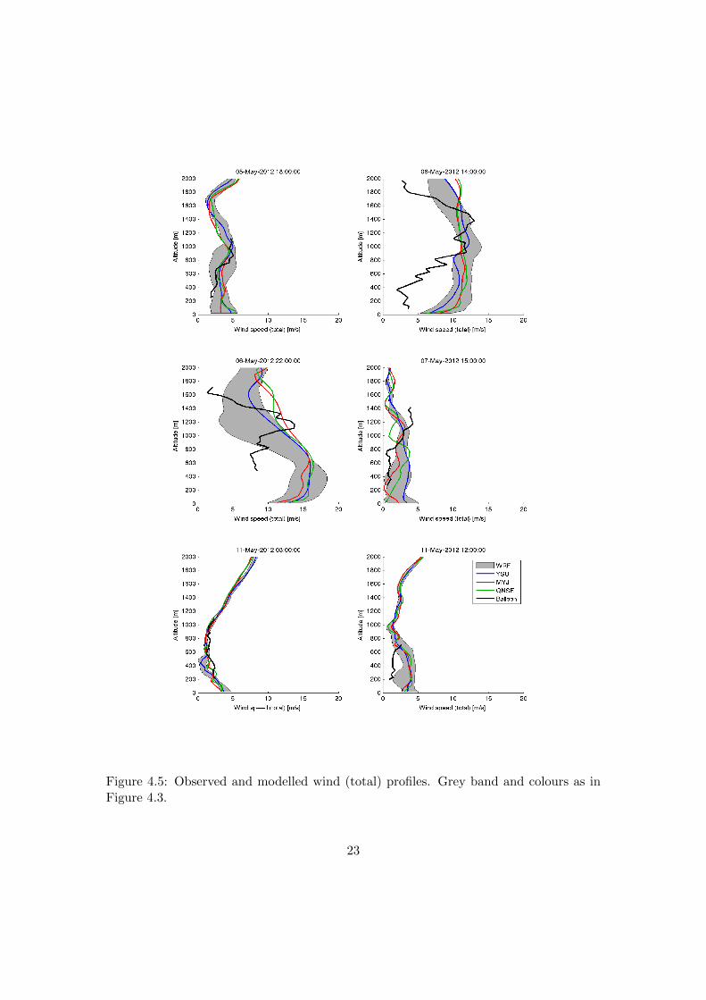
Figure 4.5: Observed and modelled wind (total) profiles. Grey band and colours as inFigure 4.3.

23

Figure 4.6: Observed and modelled potential temperature profiles. Grey band andcolours as in Figure 4.3.

24

Figure 4.7: Observed and modelled relative humidity profiles. Grey band and colours asin Figure 4.3.

25

Mean abs. error Mean bias error

Wind (u) YSU MYJ QNSE YSU MYJ QNSE

Profile 1 0.7259 1.1554 1.0781 -0.2765 -1.1554 -0.8289

Profile 2 3.3675 3.7137 3.5772 3.3675 3.6869 3.5733

Profile 3 4.4004 3.9208 4.0474 1.1609 1.2301 0.4173

Profile 4 1.9725 1.1385 2.0199 1.0097 -0.1212 0.2799

Profile 5 1.0082 1.1418 1.3047 -0.8214 -1.0042 -1.2687

Profile 6 0.8185 0.5377 0.4399 0.7788 0.5138 0.3525

Average 2.0488 1.9347 2.0779 0.8698 0.5250 0.4209

Wind (v)

Profile 1 0.7111 0.6796 0.5473 0.4511 0.3213 0.2404

Profile 2 3.0068 3.4173 3.5452 2.1320 2.4497 2.6697

Profile 3 3.4304 4.5488 4.7746 2.9552 4.5488 4.7158

Profile 4 0.7424 0.5027 1.1261 0.5635 0.3384 0.4858

Profile 5 0.6889 0.6587 0.5047 -0.2154 -0.3005 -0.1806

Profile 6 2.0594 2.1563 2.4129 2.0594 2.1563 2.4129

Average 1.7732 1.9939 2.1518 1.3243 1.5857 1.7240

Wind (total)

Profile 1 0.5609 0.9381 0.7687 0.2837 0.3234 0.0963

Profile 2 3.4914 4.0992 4.2508 3.2142 3.4867 3.6976

Profile 3 4.3992 4.9400 5.0845 3.2411 4.6842 4.5081

Profile 4 1.8861 1.0433 1.9871 0.9089 -0.2294 0.1691

Profile 5 0.5465 0.3547 0.2920 -0.4501 -0.2578 -0.1778

Profile 6 1.8598 1.9355 2.0246 1.7766 1.7634 1.9578

Average 2.1240 2.2184 2.4013 1.4957 1.6284 1.7085

Pot. temp.

Profile 1 0.5121 0.7127 0.4815 -0.0576 -0.1037 0.0872

Profile 2 1.6233 1.8864 1.7537 -1.2986 -1.4617 -1.3859

Profile 3 2.3796 2.2054 2.5422 1.8728 1.6729 2.1943

Profile 4 0.7460 1.0867 1.0296 -0.5103 -0.8620 -0.8149

Profile 5 1.0770 0.9397 1.0513 -1.0571 -0.9364 -1.0384

Profile 6 1.3554 2.0513 1.9328 -1.3554 -2.0513 -1.9328

Average 1.2822 1.4804 1.4652 -0.4010 -0.6237 -0.4817

Rel. humidity

Profile 1 20.8973 15.3314 17.0006 13.7883 1.7953 8.9100

Profile 2 12.3779 16.6247 14.9303 -9.1915 -13.1670 -12.2225

Profile 3 27.2586 26.8620 27.8343 -24.1392 -24.5274 -26.5595

Profile 4 7.0112 7.8416 8.1084 2.6060 0.5462 4.7798

Profile 5 2.9870 5.2645 4.7463 2.8050 -4.8741 -3.9295

Profile 6 34.9671 35.5742 46.9129 34.9671 35.5742 46.9129

Average 17.5832 17.9164 19.9221 3.4726 -0.7755 2.9819

Table 4.1: Mean absolute error and mean bias error for the three boundary layer schemesin model run 1.

26

4.3 Model run 2: Sea ice

In the second model run, the innermost domain lay south east of Svalbard and coveredthe part over sea ice, where the fourth balloon measured two profiles, and the islandHopen, which is however not fully resolved in WRF (Figure 2.1b). The locations of theballoon soundings are marked in Figure 3.1. Figures 4.8 to 4.12 show the observed andmodelled profiles for this case. Table 4.2 contains the mean absolute error and the meanbias error for each scheme and profile.

All schemes tend to overestimate wind speed, especially at the low levels, and unter-estimate potential temperature and relative humidity. The u component of the wind isquite correctly reproduced in the upper levels, but too high in the lower levels. The vcomponent is overestimated over the whole height of the profile. Nevertheless the slopeof the curve corresponds approximately to the observations. For total wind speed, theYSU scheme has the least bias and the least mean absolute error, although the QNSEscheme is better considering the u component.

Potential temperature is underestimated by around 2.5K in all schemes. The largestdifference between the observations and the model is found at the low levels, where itreaches up to 4K. With increasing height the curves converge and only a small differenceremains at the highest level. This corresponds well to the results from Section 4.1, whichshowed that WRF yielded too low temperatures over the sea ice flag when comparedto the ECMWF data. The negative bias of surface temperature over sea ice and hencethe errors in slope and magnitude of the temperature profile might indicate that therewas too much sea ice in the model set up. Since fractional sea ice was not included inthe model run, each grid cell was either fully covered by sea ice or not covered at all.Hence, in WRF, the according area was completely covered with sea ice, where in realitythere might have been patches of open water, which would then have lead to highertemperatures above the surface. Surface temperature was even more underestimatedby the MYJ and the QNSE scheme than by the YSU scheme, which was used for thecomparison with the ECMWF data in Section 4.1. Nevertheless, the MYJ scheme showsthe least error considering all the levels.

The relative humidity profiles are very well reproduced by the YSU scheme, in par-ticular profile 7. It only slightly underestimates the magnitude, while the other twoschemes show a high bias as well as errors in the structure of the profile. YSU alsohas the least mean absolute error and mean bias error for profile 8, although there thestructure is not as well represented as in profile 7. It seems that the underestimationof temperature in WRF does not have a high influence on relative humidity, meaningthat also specific humidity must be lower in the model than in the observations, whichis probably due to reduced latent heat flux in case of more sea ice.

27

Figure 4.8: Observed and modelled wind (u) profiles. Grey band and colours as inFigure 4.3.

Figure 4.9: Observed and modelled wind (v) profiles. Grey band and colours as inFigure 4.3.

28

Figure 4.10: Observed and modelled wind (total) profiles. Grey band and colours as inFigure 4.3.

Figure 4.11: Observed and modelled potential temperature profiles. Grey band andcolours as in Figure 4.3.

29

Figure 4.12: Observed and modelled relative humidity profiles. Grey band and coloursas in Figure 4.3.

Mean abs. error Mean bias error

Wind (u) YSU MYJ QNSE YSU MYJ QNSE

Profile 7 1.1715 0.9553 0.9004 0.3608 0.8022 0.6756

Profile 8 1.8154 2.1230 1.6786 1.5999 2.1230 1.4410

Average 1.4935 1.5391 1.2895 0.9804 1.4626 1.0583

Wind (v)

Profile 7 2.6962 2.5932 2.9433 -2.6962 -2.5932 -2.9433

Profile 8 1.3181 1.4924 1.2470 -1.3181 -1.4924 -1.2470

Average 2.0072 2.0428 2.0952 -2.0072 -2.0428 -2.0952

Wind (total)

Profile 7 1.5763 1.8533 1.9428 1.5574 1.8533 1.9428

Profile 8 2.0156 2.5336 1.8690 2.0156 2.5336 1.8185

Average 1.7959 2.1935 1.9059 1.7865 2.1935 1.8807

Pot. temp.

Profile 7 2.7728 2.5933 2.7267 -2.7728 -2.5933 -2.7267

Profile 8 2.6798 2.4059 2.6801 -2.6798 -2.4059 -2.6801

Average 2.7263 2.4996 2.7034 -2.7263 -2.4996 -2.7034

Rel. humidity

Profile 7 2.0766 11.2449 7.0854 -0.9256 -10.4236 -5.2106

Profile 8 5.3667 7.5444 9.2024 -2.4527 -7.5444 -8.7000

Average 3.7216 9.3947 8.1439 -1.6892 -8.9840 -6.9553

Table 4.2: Mean absolute error and mean bias error for the three boundary layer schemesin model run 2.

30

4.4 Timeseries

To analyse the performance of WRF over the time of the simulation period, timeserieswere extracted from the model at the locations of three weather stations situated in NyAlesund, Verlegenhuken and Hopen. The locations are depicted in Figure 4.13. Theweather station in Ny Alesund is run by the Alfred Wegener Institute (AWI) and thePolar Institute Paul Emile Victor (IPEV), and takes measurements every minute. Thestations in Verlegenhuken and Hopen are run by the Norwegian Meteorological Insti-tute (met.no) and take measurements every six hours. Winds are measured 10m aboveground, while temperature and relative humidity are measured 2m above ground. Inorder to get comparable correlation coefficients, the timeseries from Ny Alesund wasinterpolated to 6h intervals. Likewise, the timeseries produced by WRF, which had atemporal resolution between 1s and 20s, depending on the time step, were interpolatedto 6h intervals. The stations in Ny Alesund and Verlegenhuken were included in thethird domain of the first model run, while the station on Hopen was included in thethird domain of the second model run.

The meteorological timeseries are generally well reproduced by WRF. The correla-tion is high and the p value is below 0.01 for every parameter and every station, meaningthat all the correlations are statistically significant different from 0. Temperature is the

Figure 4.13: Locations of the weather stations.

31

parameter that has the highest correlation for most of the stations and schemes. Ithas however also quite a large bias. All the schemes overestimate temperature in NyAlesund and Verlegenhuken (especially the very low temperatures) and highly underes-timate it on Hopen. On Hopen, this might be connected to fog that occurred in realitybut remained unrepresented in the model, together with the fact that seaice was proba-bly overrepresented in this area. Fog could also explain the lower daily variation in theobservations compared to the model timeseries. For temperature, the MYJ scheme hasthe highest correlation, while the YSU scheme has the least mean absolute error and theleast bias.

All the schemes show very strong southerly winds on 6 May 2011 in Ny Alesund,which did not occur in reality. Otherwise, the winds are very reasonably reproduced byWRF, except for a small overestimation of the u component on Hopen in the end of theperiod. The QNSE scheme has the highest correlation for total wind speed as well asthe lowest mean absolute error and bias.

Relative humidity is the parameter with the lowest correlation between the model andthe observations. Especially remarkable are the values exceeding 100% on Hopen around4 May and 7 May. The problem might be caused by an overestimation of atmosphericpressure, which leads to higher vapour pressure when calculating relative humidity fromthe mixing ratio. The QNSE scheme correlates best with the observations and has theleast mean absolute error, but the YSU scheme shows a lower bias.

4.4.1 Wind roses

Figure 4.17 to 4.19 show wind roses for the different weather stations and the three ABLschemes at the given location. The main wind direction in Ny Alesund is northwesterlyand southeasterly, following the direction of Kongsfjorden, where Ny Alesund is located.In WRF, the winds are turned by around 30◦ clockwise and the wind speeds of thenorthwesterly winds are much higher. Furthermore, there is a strong southerly compo-nent that cannot be found in the observations. This corresponds to the positive peakin the v component in Figure 4.14 on 6 May that was mentioned above. In Verlegen-huken, the winds are mainly southeasterly. There is also a smaller component from thesouthwest, but almost no winds from the northern two quadrants. In contrast, all theschemes in WRF have a strong northwesterly component with high wind speeds. Thispeak can be found on the evening of 8 May in the original data of u and v (not shown),where u was around 5m/s and v reached under -10m/s for a short period. Unfortu-nately, it got lost in the interpolation to 6h intervals. On Hopen, the observations revealmain wind directions from the southwest and the northeast. In WRF, the componentfrom the northeast is almost completely missing, and the southwesterly component isunderestimated in proportion as well as in speed. Winds coming from the north areoverrepresented instead. This can also be seen in the negative bias of the v componentin Table 4.3.

32

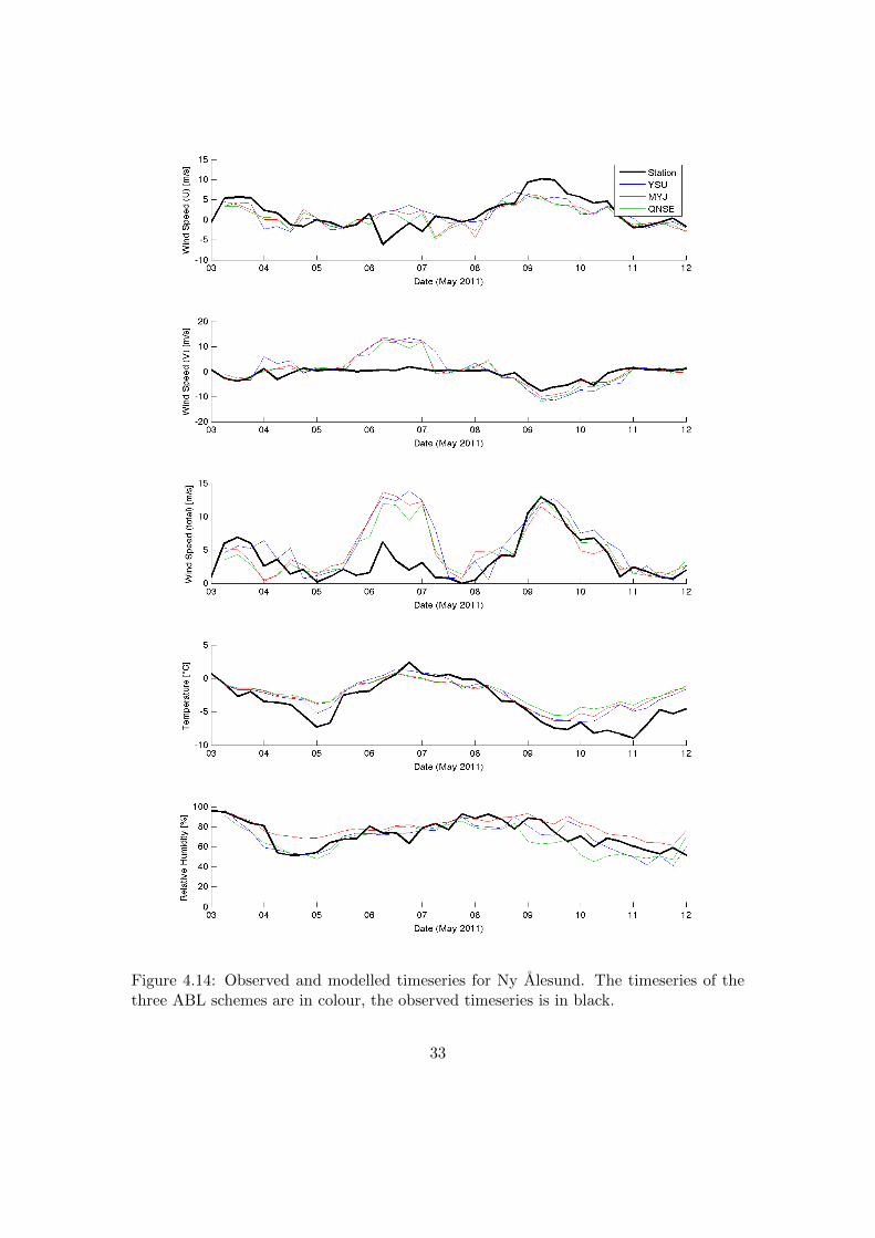
Figure 4.14: Observed and modelled timeseries for Ny Alesund. The timeseries of thethree ABL schemes are in colour, the observed timeseries is in black.

33

Figure 4.15: Observed and modelled timeseries for Verlegenhuken. Colours as in Fig-ure 4.14.

34

Figure 4.16: Observed and modelled timeseries for Hopen. Colours as in Figure 4.14.

35

(a) AWIPEV station (b) YSU scheme

(c) MYJ scheme (d) QNSE scheme

Figure 4.17: Observed and modelled wind roses for Ny Alesund in the period 3 May2011 00:00 UTC to 12 May 2011 00:00 UTC. Colours indicate wind speed (m/s).

36

(a) Met.no station (b) YSU scheme

(c) MYJ scheme (d) QNSE scheme

Figure 4.18: Observed and modelled wind roses for Verlegenhuken in the period 3 May2011 00:00 UTC to 12 May 2011 00:00 UTC. Colours indicate wind speed (m/s).

37

(a) Met.no station (b) YSU scheme

(c) MYJ scheme (d) QNSE scheme

Figure 4.19: Observed and modelled wind roses for Hopen in the period 3 May 201100:00 UTC to 12 May 2011 00:00 UTC. Colours indicate wind speed (m/s).

38

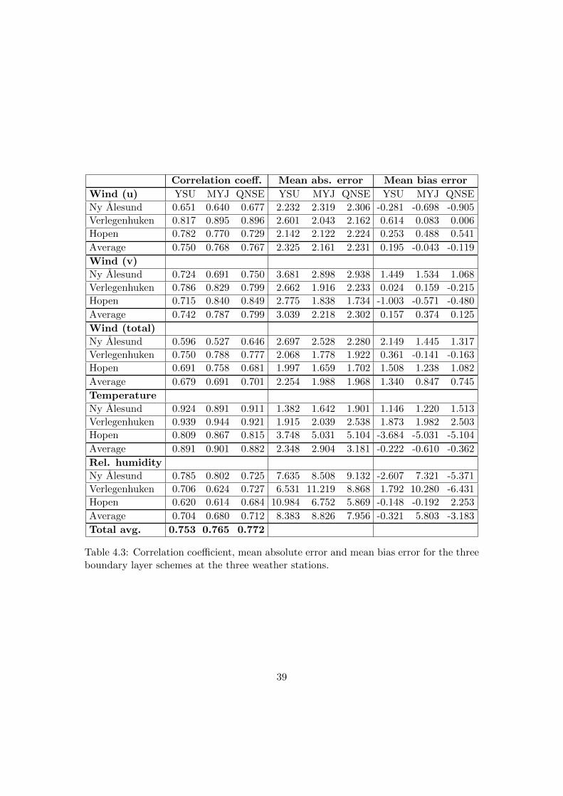
Correlation coeff. Mean abs. error Mean bias error

Wind (u) YSU MYJ QNSE YSU MYJ QNSE YSU MYJ QNSE

Ny Alesund 0.651 0.640 0.677 2.232 2.319 2.306 -0.281 -0.698 -0.905

Verlegenhuken 0.817 0.895 0.896 2.601 2.043 2.162 0.614 0.083 0.006

Hopen 0.782 0.770 0.729 2.142 2.122 2.224 0.253 0.488 0.541

Average 0.750 0.768 0.767 2.325 2.161 2.231 0.195 -0.043 -0.119

Wind (v)

Ny Alesund 0.724 0.691 0.750 3.681 2.898 2.938 1.449 1.534 1.068

Verlegenhuken 0.786 0.829 0.799 2.662 1.916 2.233 0.024 0.159 -0.215

Hopen 0.715 0.840 0.849 2.775 1.838 1.734 -1.003 -0.571 -0.480

Average 0.742 0.787 0.799 3.039 2.218 2.302 0.157 0.374 0.125

Wind (total)

Ny Alesund 0.596 0.527 0.646 2.697 2.528 2.280 2.149 1.445 1.317

Verlegenhuken 0.750 0.788 0.777 2.068 1.778 1.922 0.361 -0.141 -0.163

Hopen 0.691 0.758 0.681 1.997 1.659 1.702 1.508 1.238 1.082

Average 0.679 0.691 0.701 2.254 1.988 1.968 1.340 0.847 0.745

Temperature

Ny Alesund 0.924 0.891 0.911 1.382 1.642 1.901 1.146 1.220 1.513

Verlegenhuken 0.939 0.944 0.921 1.915 2.039 2.538 1.873 1.982 2.503

Hopen 0.809 0.867 0.815 3.748 5.031 5.104 -3.684 -5.031 -5.104

Average 0.891 0.901 0.882 2.348 2.904 3.181 -0.222 -0.610 -0.362

Rel. humidity

Ny Alesund 0.785 0.802 0.725 7.635 8.508 9.132 -2.607 7.321 -5.371

Verlegenhuken 0.706 0.624 0.727 6.531 11.219 8.868 1.792 10.280 -6.431

Hopen 0.620 0.614 0.684 10.984 6.752 5.869 -0.148 -0.192 2.253

Average 0.704 0.680 0.712 8.383 8.826 7.956 -0.321 5.803 -3.183

Total avg. 0.753 0.765 0.772

Table 4.3: Correlation coefficient, mean absolute error and mean bias error for the threeboundary layer schemes at the three weather stations.

39

5 Discussion

5.1 Wind

WRF had a tendency to overestimate surface wind speeds, especially in case of strongwinds (see profile 2 and 3 in Figure 4.3 to 4.5 and profile 1 in Figure 4.8 to 4.10). Theseresults correspond to a study conducted by Claremar et al. (2012), which comparedthe Polar WRF model to observations from AWS placed on three Svalbard glaciers andfound the same tendency of WRF to overestimate the highest wind speeds. However,since their AWS measured wind speed at a height below 10m, they used a correctionbased on Monin-Obukhov theory to calculate wind speed at 10m. This correction wasconstant and might, as mentioned by the authors, have led to too low wind speeds incase of more neutral stability, which is expected at high wind speeds. Nevertheless, thefindings are supported by studies made by Kilpelainen et al. (2011) and Kilpelainenet al. (2012), which showed that wind speeds in Kongsfjorden were overestimated byWRF in the lowest levels. Kilpelainen et al. (2012) also found that the average modelledlow level jet was deeper and stronger than the average observed low level jet. In thisstudy, the model did not show any low level jet, even though it was found twice in theobservations.

5.2 Temperature

WRF highly underestimated the temperatures measured over sea ice to the east of Sval-bard, in particular at the surface. As mentioned in Section 4.3, the bias is most probablydue to an overrepresentation of sea ice in the WRF model setup. Sensitivity tests includ-ing one model run with complete sea ice coverage and one model run with open sea onlyconfirmed that temperatures at low levels strongly depend on whether sea ice is presentor not. In further investigations it would therefore make sense to include fractional seaice in the model, maybe even together with varying sea ice and SST.

Moreover, WRF did not manage to capture the inversions observed in profile 2 and3 in Figure 4.6. This problem has been encountered before. Molders and Kramm(2010), who ran WRF for a five day cold weather period in Alaska, found that WRF hasdifficulties in capturing the full strength of the surface temperature inversion that wasobserved during that period. Similar results were found in the study by Kilpelainen et al.(2012), where WRF reproduced only half the amount of inversions that were found inthe observations, and thereby often underestimated its depth and strength. Molders andKramm (2010) suggest that, since low wind speeds to no wind are favourable for inversionformation, WRF’s overestimation of wind speed might partly explain the difficulties incapturing (the strength of) inversions. Also, elevated inversions are often connected to

40

low level jets (Andreas et al., 2000), thus the difficulties in capturing inversions mightexplain the absence of low level jets.

5.3 Relative humidity

Studies by Steeneveld et al. (2008) and Mayer et al. (2012a) showed that local ABLschemes produced shallower and moister boundary layers than nonlocal schemes. In thisstudy, all the schemes mostly showed a shallower and moister ABL than the observations.However, the two local schemes MYJ and QNSE in average produced lower verticalrelative humidity profiles than the nonlocal YSU scheme (see bias in Table 4.1 and4.2). In contrast, for the timeseries it is the MYJ scheme that most often showed thehighest relative humidity, while the QNSE scheme had the lowest relative humidity(bias in Table 4.3). WRF generally had the most difficulties in reproducing the relativehumidity profiles in the cases with strong winds (profile 2 and 3 in Figures 4.5 and 4.7).It highly underestimated relative humidity at the location of the low level jet.

5.4 Parameterisation schemes

The YSU scheme without doubt showed the best overall performance when compared tothe CMET balloon profiles. This stands in contrast to the results found by Kilpelainenet al. (2012), where the YSU scheme yielded the largest errors in the vertical profiles.When looking at the timeseries, the MYJ and the QNSE scheme showed smaller absoluteerrors than the YSU scheme for all parameters except temperature. The QNSE schemeyielded the smallest absolute errors for relative humidity and total wind speed, whilethe MYJ scheme was better considering the u and v component of the wind separately.Additionally, the average correlation coefficient for each parameter was highest for ei-ther the MYJ or the QNSE scheme, the QNSE scheme having the highest correlationcoefficient in total. This agrees with the results found by Claremar et al. (2012), whichshowed that the QNSE scheme outperformed the MYJ scheme when compared to mea-surements from AWS. It leads us to the conclusion that the QNSE scheme is especiallypowerful at the lower levels, where the timeseries were measured, while having moredifficulties reproducing vertical profiles. The YSU scheme shows the best performancefor the vertical profiles. However, the differences between the schemes in total were verysmall, and, moreover, the observational period was rather short, including only sevendays. The statistical significance of the results found might therefore be limited.

41

6 Future work

The results presented in Section 4.3 show that WRF, when compared to vertical profilesmeasured over sea ice, underestimated temperature and overestimated wind speed, es-pecially at low levels. These results suggest to have a closer look at the implementationof sea ice into WRF in further investigations. Even though the sea ice flag from theECMWF data seems to agree fairly well with the real sea ice flag seen on a satellite pic-ture that was taken at that time, areas of polynyas and leads that can be recognised onthe satellite picture were represented as homogeneous sea ice in the model. One optionis to remove excessive sea ice manually, as, e.g., in Mayer et al. (2012b). Another oradditional option is to use fractional sea ice. In the ECMWF data, grid cells with leadsand polynyas are represented as only partly covered by sea ice (a fraction smaller thanone). Such a fractional sea ice option is available for WRF version 3.1.1 and higher. Yet,in this study we ran the model without the option of fractional sea ice and thereforeassumed that each grid cell within the sea ice flag was fully covered by sea ice. Thiscould explain the errors in the profiles of Section 4.3 and needs to be further investi-gated. However, it is difficult to implement fractional sea ice accurately. The amount ofsea ice in a grid cell is varying in time through sea ice formation, break up and drifting,where drifting is the dominant process in late spring. Therefore, it is not advisableto leave the sea ice field constant during the simulation time in case the fractional seaice option is used. However, since WRF is a meteorological model, it does not includemodelling of ocean currents and hence drifting of sea ice. The presence of sea ice onlydepends on whether the SST is above or below the freezing point of water. An optionto overcome this problem is to update the sea ice field and the SST in a certain interval(e.g., six hours) with data from observations or reanalyses, as in Kilpelainen et al. (2012).

Polar WRF was developed especially for the Arctic and Antarctic, with a selectionof physical parameterisations best suited for polar regions. In further investigations itmight be interesting to see whether Polar WRF performs better than the standard WRFin our case. However, one of the major advantages of Polar WRF was the treatmentof fractional sea ice, which has not been available before, but is now also included inthe standard WRF. Accordingly, studies by Kilpelainen et al. (2012) showed that thedifferences between the standard WRF version 3.1.1 and its corresponding polar versionwere marginal. Standard WRF even captured the wind and temperature profiles slightlybetter than Polar WRF.

Finally, it would probably also be better to look at specific humidity in future analysesinstead of (or in addition to) relative humidity, since relative humidity might be biasedthrough pressure and temperature.

42

7 Acknowledgements

I would like to thank Lars Robert Hole for accepting me as an intern at met.no. I amvery happy to have been given the chance to work in Bergen and participate in thisproject. Also thanks for the many helpful talks and discussions and the suggestion toapply for a course on Svalbard. Thanks to Paul Voss for the supportive discussionsvia skype and the help in writing the report. Thanks to Marius Jonassen for helpingin getting familiar with WRF and its brother WPS and for always having an answerand being ready to help when there was a problem with the model. Thanks to SiegridDebatin from AWIPEV for providing us with radiosonde and weather station data fromNy Alesund. Big thanks to Aslaug Valved and Aurora Stenmark for being awesomefriends and WRF buddies. Takk til Bergen for et fantastisk halvt ar.

43

Bibliography

E. L. Andreas, K. J. Claffey, and A. P. Makshtas. Low-level atmospheric jets andinversions over the western weddell sea. Boundary-Layer Meteorology, 97:459–486,2000.

R. Bintanja, R. G. Graversen, and W. Hazeleger. Arctic winter warming amplified by thethermal inversion and consequent low infrared cooling to space. Nature Geoscience,4:758–761, 2011.

D. H. Bromwich, K. M. Hines, and L.-S. Bai. Development and testing of polar weatherresearch and forecasting model: 2. arctic ocean. J. Geophys. Res., 114:D08122, 2009.

F. Chen and J. Dudhia. Coupling an advanced land-surface/ hydrology model with thepenn state/ ncar mm5 modeling system. part i: Model description and implementa-tion. Mon. Wea. Rev., 129:569–585, 2001.

B. Claremar, F. Obleitner, C. Reijmer, V. Pohjola, A. Waxegard, F. Karner, and A. Rut-gersson. Applying a mesoscale atmospheric model to svalbard glaciers. Advances inMeteorology, 2012:22 pages, 2012. Article ID 321649.

J. Dudhia. Numerical study of convection observed during the winter monsoon experi-ment using a mesoscale two-dimensional model. J. Atmos. Sci., 46:3077–3107, 1989.

K. M. Hines and D. H. Bromwich. Development and testing of polar weather researchand forecasting (wrf) model. part i: Greenland ice sheet meteorology*. Mon. Wea.Rev., 136:1971–1989, 2008.

S.-Y. Hong, J. Dudhia, and S.-H. Chen. A revised approach to ice microphysical processesfor the bulk parameterization of clouds and precipitation. Mon. Wea. Rev., 132:103–120, 2004.

S.-Y. Hong, Y. Noh, and J. Dudhia. A new vertical diffusion package with an explicittreatment of entrainment processes. Mon. Wea. Rev., 134:23182341, 2006.

J. T. Houghton, Y. Ding, D. J. Griggs, M. Noguer, P. J. van der Linden, X. Dai,K. Maskel, C. A. Johnson, and Eds. Climate Change 2001: The Scientific Basis.Cambridge University Press, 2001.

Z. I. Janjic. The step-mountain coordinate: physical package. Mon. Wea. Rev., 118:1429–1443, 1990.

Z. I. Janjic. The surface layer in the ncep eta model. In Eleventh Conference on Numer-ical Weather Prediction, pages 354–355, Norfolk, VA, 19-23 August 1996. AmericanMeteorological Society.

44

Z. I. Janjic. Nonsingular implementation of the melloryamada level 2.5 scheme in thencep meso model. NCEP Office Note, No. 437:61 pp, 2002.

J. S. Kain. The kain-fritsch convective parameterization: An update. J. Appl. Meteor.,43:170–181, 2004.

T. Kilpelainen, T. Vihma, and H. Olafsson. Modelling of spatial variability and topo-graphic effects over arctic fjords in svalbard. Tellus A, 63(2):223–237, 2011.

T. Kilpelainen, T. Vihma, M. Manninen, A. Sjoblom, E. Jakobson, T. Palo, and M. Ma-turilli. Modelling the vertical structure of the atmospheric boundary layer over arcticfjords in svalbard. Q. J. R. Meteorol. Soc., 2012.

G. Livik. An observational and numerical study of local winds in kongsfjorden, spits-bergen, 2011. Master Thesis at the University of Bergen.

J. Lu and M. Cai. Quantifying contributions to polar warming amplification in anidealized coupled general circulation model. Climate Dynamics, 34:669–687, 2010.

E. Makiranta, T. Vihma, A. Sjoblom, and E.-M. Tastula. Observations and modellingof the atmospheric boundary layer over sea-ice in a svalbard fjord. Boundary-LayerMeteorology, 140:105–123, 2011.

S. Mayer, A. Sandvik, M. Jonassen, and J. Reuder. Atmospheric profiling with theuas sumo: a new perspective for the evaluation of fine-scale atmospheric models.Meteorology and Atmospheric Physics, 116:15–26, 2012a.

S. Mayer, M. Jonassen, A. Sandvik, and J. Reuder. Profiling the arctic stable boundarylayer in advent valley, svalbard: Measurements and simulations. Boundary-LayerMeteorology, 143:507–526, 2012b.

G. L. Mellor and T. Yamada. Development of a turbulence closure model for geophysicalfluid problems. Rev. Geophys. Space Phys., 20:851–875, 1982.

A. C. Mentzoni. Flexpart validation with the use of cmet balloons, 2011. Master Thesisat the University of Bergen.

E. J. Mlawer, S. J. Taubman, P. D. Brown, M. J. Iacono, and S. A. Clough. Radiativetransfer for inhomogeneous atmospheres: Rrtm, a validated correlated-k model for thelongwave. J. Geophys. Res., 102:16663–16682, 1997.

N. Molders and G. Kramm. A case study on wintertime inversions in interior alaskawith wrf. Atmospheric Research, 95(23):314–332, 2010.

P. O. G. Persson, C. W. Fairall, E. L. Andreas, P. S. Guest, and D. K. Perovich. Measure-ments near the atmospheric surface flux group tower at sheba: Near-surface conditionsand surface energy budget. J. Geophys. Res., 107:8045–8079, 2002.

45

E. E. Riddle, P. B. Voss, A. Stohl, D. Holcomb, D. Maczka, K. Washburn, and R. W.Talbot. Trajectory model validation using newly developed altitude-controlled bal-loons during the international consortium for atmospheric research on transport andtransformations 2004 campaign. J. Geophys. Res., 111:D23S57, 2006.

A. Rinke, K. Dethloff, J. Cassano, J. Christensen, J. Curry, P. Du, E. Girard, J.-E.Haugen, D. Jacob, C. Jones, M. Kltzow, R. Laprise, A. Lynch, S. Pfeifer, M. Ser-reze, M. Shaw, M. Tjernstrm, K. Wyser, and M. agar. Evaluation of an ensemble ofarctic regional climate models: spatiotemporal fields during the sheba year. ClimateDynamics, 26:459–472, 2006.

W. Skamarock, J. Klemp, J. Dudhia, D. Gill, D. Barker, M. Duda, H. X. Y.,and W. Wang. A description of the advanced research wrf version 3, 2008.NCAR/TN:475+STR.

G. J. Steeneveld, T. Mauritsen, E. I. F. de Bruijin, J. Vila-Guerau de Arellano, G. Svens-son, and A. A. M. Holtslag. Evaluation of limited-area models for the representationof the diurnal cycle and contrasting nights in cases-99. J. Appl. Meteor. Climatol., 47:869–887, 2008.

A. Stohl, G. Wotawa, P. Seibert, and H. Kromp-Kolb. Interpolation errors in wind fieldsas a function of spatial and temporal resolution and their impact on different types ofkinematic trajectories. J. Appl. Meteorol., 34:2149–2165, 1995.

A. Stohl, M. Hittenberger, and G. Wotawa. Validation of the lagrangian particle disper-sion model flexpart against large-scale tracer experiment data. Atmospheric Environ-ment, 32(24):4245–4264, 1998.

S. Sukoriansky, B. Galperin, and V. Perov. A quasi-normal scale elimination modelof turbulence and its application to stably stratified flows. Nonlinear Processes inGeophysics, 13:9–22, 2006.

P. B. Voss, R. A. Zaveri, F. M. Flocke, H. Mao, T. P. Hartley, P. DeAmicis, I. Deonandan,G. Contreras-Jimenez, O. Martınez-Antonio, M. Figueroa Estrada, D. Greenberg,T. L. Campos, A. J. Weinheimer, D. J. Knapp, D. D. Montzka, J. D. Crounse, P. O.Wennberg, E. Apel, S. Madronich, and B. de Foy. Long-range pollution transportduring the milagro-2006 campaign: a case study of a major mexico city outflow eventusing free-floating altitude-controlled balloons. Atmos. Chem. Phys., 10:7137–7159,2010.

P. B. Voss, L. R. Hole, E. Helbling, and T. Roberts. Continuous in-situ soundings in thearctic boundary layer: A new atmospheric measurement technique using controlledmeteorological balloons. Journal of Intelligent & Robotic Systems, pages 1–9, 2012.

46