1

Evaluation of the wind farm parameterization in the Weather

Research and Forecasting model (version 3.8.1) with meteorological

and turbine power data

Joseph C. Y. Lee and Julie K. Lundquist1,2

1Department of Atmospheric and Oceanic Sciences, University of Colorado, UCB 311, Boulder, CO 80309, USA 5 2National Renewable Energy Laboratory, Golden, CO, USA

Correspondence to: Joseph C. Y. Lee (chle6805@coloardo.edu)

Abstract. Forecasts of wind power production are necessary to facilitate the integration of wind energy into power grids, and

these forecasts should incorporate the impact of wind turbine wakes. This paper focuses on a case study of four diurnal

cycles with significant power production, and assesses the skill of the wind farm parameterization (WFP) distributed with the 10

Weather Research and Forecasting (WRF) model version 3.8.1, as well as its sensitivity to model configuration. After

validating the simulated ambient flow with observations, we quantify the value of the WFP as it accounts for wake impacts

on power production of downwind turbines. We also illustrate that a vertical grid with nominally 12-m vertical resolution is

necessary for reproducing the observed power production, with statistical significance. Further, the WFP overestimates wake

effects and hence underestimates downwind power production during high wind speed and low turbulence conditions. We 15

also find the WFP performance is independent of atmospheric stability, the number of wind turbines per model grid cell, and

the upwind-downwind position of turbines. Rather, the ability of the WFP to predict power production is most dependent on

the skill of the WRF model in simulating the ambient wind speed.

1 Introduction

In recent years, numerical weather prediction (NWP) models have become an indispensable tool in the wind energy 20

industry, not only in day-to-day wind energy production forecasts (Wilczak et al., 2015), but also to support wide-scale wind

power penetration (Marquis et al., 2011) and wind resource assessment. To forecast power production accurately at wind

farms, the simulation tools should resolve all physical processes relevant to the wind field, including possible impacts of the

wind turbines themselves. Consequently, including the effects of wind farms in NWP models can improve power production

forecasts. 25

Researchers have developed various methods to numerically represent wind farms. Via large-eddy simulations (LES),

some investigators assess the meteorological impacts of wind turbines as well as power production (Abkar and Porté-Agel,

2015b; Aitken et al., 2014; Calaf et al., 2010; Churchfield et al., 2012; Jimenez et al., 2007; Mirocha et al., 2014; Na et al.,

2

2016; Sharma et al., 2016; Wu and Porté-Agel, 2011). Simulating wind turbines and their effects in LES is, while useful,

computationally expensive, making wind-farm-scale simulations unreasonable in an operational setting. 30

At coarser spatial scales, suitable for global, synoptic or mesoscale models, numerically representing wind turbine

effects may involve unrealistic assumptions. For example, researchers have used exaggerated surface roughness to represent

the wind speed (WS) reduction caused by wind farms in a global model (Barrie and Kirk-Davidoff, 2010; Frandsen et al.,

2009; Keith et al., 2004). Similarly, the analytical wind park model of Emeis and Frandsen (1993) considers both the

downward momentum flux and the momentum loss due to surface roughness. The revised model by Emeis (2010) accounts 35

for the spatially-averaged momentum-extraction coefficient by turbines, and the parameters become atmospheric-stability

dependent. However, these models omit the consideration of turbine-scale interactions between the hub and the surface

(Abkar and Porté-Agel, 2015a; Fitch et al., 2012, 2013b).

Aside from indirectly representing wind turbines via exaggerated roughness, another common approach is to use the

turbine power curve to deduce elevated drag and turbulence production of wind turbines. A power curve illustrates the 40

relationship between inflow WS at hub height and power production of a particular turbine model. This method can model

meteorological impacts of wind turbines and the impact of turbine drag force (Baidya Roy, 2011; Blahak et al., 2010). Based

on this technique, Fitch et al. (2012) added the consideration of the turbine thrust coefficient to simulate both turbine drag

and power loss.

In the wind farm parameterization (WFP) of the Weather Research and Forecasting (WRF) model, wind turbines in each 45

model grid cell are collectively represented as a turbulence source and a momentum sink within the vertical levels of the

turbine rotor disk (Fitch et al., 2012). A fraction of the kinetic energy extracted by the virtual wind turbines is converted to

power, and the turbulence generation is derived from the difference between the thrust and power coefficients. In the WFP

scheme, the use of the WS-dependent thrust coefficients accounts for the effects of local wind drag on wind energy

extraction as well as on power estimation. The WRF WFP offers flexibility, where users can modify the parameters of a 50

turbine model, such as its hub height, rotor diameter, power curve and thrust coefficients, and does not require other

empirically-derived parameters. By simulating wind farms in a mesoscale weather model, WRF users can simulate

aggregated effects of wind turbine wakes and thus the effects of power production of downwind turbines.

An approach similar to the WRF WFP proposed by Abkar and Porté-Agel (2015a), relies on an extra parameter, the

ratio of the freestream velocity to the horizontally-averaged hub-height velocity of a turbine-containing grid cell. This ratio 55

depends on various factors such as the wind farm density and layout, and requires preliminary simulation results (Abkar and

Porté-Agel, 2015a). Therefore, the publicly-available WFP in the WRF model is chosen in this project for observed power

comparison. On the other hand, the explicit wake parameterization (EWP) recently designed by Volker et al. (2015) uses

classical wake theory to describe the unresolved wake expansion. Both the WRF WFP and the EWP average the drag force

within grid cells. Nevertheless, users of the EWP need to adjust the length scales that determine wake expansion in the EWP 60

for different situations.

3

In this paper, we evaluate the WFP in the WRF model via comparison to turbine power production data. The WRF WFP

has been widely used to assess the impacts, of both onshore and offshore wind farms, at different spatial scales, and in

different stability regimes (Eriksson et al., 2015; Fitch et al., 2013a, 2013b; Jiménez et al., 2015; Lee and Lundquist, 2017;

Miller et al., 2015; Vanderwende et al., 2016; Vanderwende and Lundquist, 2016; Vautard et al., 2014). While WFP 65

predictions have been compared to power production in offshore wind farms for a limited set of wind speeds (Jiménez et al.,

2015), here we explore a range of WS, wind direction (WD), turbulence, and atmospheric stability conditions. The large

range of wind conditions induces spatially- and temporally-diverse power production, thereby providing a basis for a

comprehensive evaluation of the WFP. The uniqueness of this project lies in the in-depth assessment of the WRF WFP

performance in forecasting and simulating wind energy of a sizable onshore wind farm, using observed power production 70

data.

We describe the observation data and the model design in Section 2. In Section 3, we evaluate the simulations by

comparison to meteorological and power generation data. We close with a statistical examination and a proposal of

improvements on the WRF WFP in Section 4.

2 Data and Methods 75

2.1 Observations

The 2013 Crop Wind Energy eXperiment (CWEX-13) took place in central Iowa at a 200-turbine wind farm to

quantify far-wake impacts of multiple rows of turbines (Lundquist et al., 2014). In CWEX-13, measurements from seven

surface flux stations, a radiometer, three profiling lidars and a scanning lidar were collected. This campaign was a

component of the larger CWEX project, which explored the interactions of wind turbines with crops, surface fluxes and 80

near-surface flows in different atmospheric stability regimes in flat terrain (Rajewski et al., 2013). Research facilitated by the

CWEX projects include: diurnal changes in observed turbine wakes (Rhodes and Lundquist, 2013), turbine interactions with

moisture and carbon dioxide fluxes (Rajewski et al., 2014), LES modelling of turbine wakes in changing stability regimes

(Mirocha et al., 2015), nocturnal low-level jet (LLJ) occurrences (Vanderwende et al., 2015), diurnal changes of the

microclimate near wind turbines (Rajewski et al., 2016), multiple-wake interactions (Bodini et al., 2017), the evolution of 85

turbine wakes during the evening transition (Lee and Lundquist, 2017) and coupled mesoscale-microscale modelling

(Muñoz-Esparza et al., 2017).

This wind farm consists of 200 wind turbines, represented by the red dots in Fig. 1. Half of the wind turbines in the

wind farm are General Electric (GE) 1.5-MW super-long extended (SLE) model, and the other half are GE 1.5-MW extra-

long extended (XLE) model (Rajewski et al., 2013). The cut-in and cut-out speeds of the SLE model are 3.5 and 25 m s-1 90

respectively, and the rated speed is 14 m s-1. The XLE model has lower rated and cut-out wind speeds, at 11.5 and 20 m s-1.

The hub height of both models is 80 m; the rotor diameters of the SLE and the XLE model are 77 and 82.5 m respectively.

For simplicity, references to the rotor diameter (D) herein refer to the 77-m rotor diameter. Power generated by each turbine

4

is recorded by the Supervisory Control and Data Acquisition (SCADA) system every 10 minutes, and we sum up the power

production of all turbines for wind-farm production for each 10-min period. 95

Observations of the wind profile are collected by a profiling lidar and a scanning lidar. The WINDCUBE v1 (WC)

profiling lidar (yellow square in Fig. 1), is located 528 m, or 6.3 D, south of the nearest turbine. The WC lidar measures

winds at about 0.25 Hz from 40 to 220 m above ground level (AGL) every 20 m via the Doppler beam swinging (DBS)

method. The WC lidar derives wind components by measuring radial velocities using Doppler beam swinging at an azimuth

angle of 28°. Note that the WC-observed turbulence parameters, turbulence kinetic energy (TKE) and turbulence intensity 100

(TI), are derived from the variances of the three wind components in two-min intervals, hence not representing small-scale

turbulence. The turbulence parameters are defined by:

𝑇𝐾𝐸 = 1

2(𝜎𝑢

2 + 𝜎𝑣2 + 𝜎𝑤

2 ), (1)

𝑇𝐼 = √𝜎𝑢

2+𝜎𝑣2

𝑈, (2)

where 𝜎2 are the 2-min averaged variances of the 𝑢, 𝑣, and 𝑤 wind components, and 𝑈 is the mean horizontal WS (Stull, 105

1988). In CWEX-11, wind turbine wake measurements at a different location in this wind farm were collected with these

instruments (Rhodes and Lundquist 2013), while the error in these lidar measurements due to inhomogeneous flow were

explored by Bingöl et al. (2009) and Lundquist et al. (2015).

The WINDCUBE 200S scanning lidar (green square in Fig. 1), is positioned 437 m, or 5.7 D, north of the nearest

turbine row. The 200S lidar scanning strategy included velocity azimuth display (VAD) scans that measures winds from 110

~100 to ~4800 m AGL nominally every 50 m for every 3 minutes. We use the 200S 75-degree-elevation scans

(Vanderwende et al., 2015) to estimate horizontal winds every 30 minutes to verify the simulated winds in the boundary

layer. Since the dominant wind directions during the campaign are south-easterly to south-westerly (Vanderwende et al.,

2015), some of the 200S measurements below the rotor top (about 120 m AGL) could be influenced by turbine wakes during

conditions, in which wakes persist longer than 5 D downwind from the turbine (Bodini et al., 2017). On the other hand, WC 115

measurements are largely unaffected by turbine wakes except when WD is east of 150°. The closest upwind turbine during

this simulation period was located over 2.7 km (33 D) to the southeast.

Surface flux station measurements can also quantify model skill. The surface flux station of interest (purple square in

Fig. 1), is located 681 m, or 8.8 D, south of the closest turbine. At 8 m AGL, the station measures 20-Hz winds via a CSAT3

sonic anemometer, as well as virtual temperature and water vapour density via a HMP45C probe. After tilt-correction 120

(Wilczak et al., 2001), we calculate surface sensible heat flux using a 30-min averaging time period. The Obukhov length (𝐿)

categorizes atmospheric stability conditions:

𝐿 = −𝑇𝑣̅̅ ̅𝑢∗

3

𝑘𝑔(𝑤′𝑇𝑣′̅̅ ̅̅ ̅̅ ̅̅ )𝑠, (3)

where 𝑇�̅� is the mean virtual temperature, 𝑢∗ is the frictional velocity, 𝑘 is the von Karman constant, 𝑔 is the gravity

acceleration, and (𝑤′𝑇𝑣′̅̅ ̅̅ ̅̅ ̅)𝑠 is the surface virtual temperature flux calculated from the 20-Hz measurements (Stull, 1988). 125

5

Positive surface sensible heat flux and Obukhov Length ratio (𝑧 𝐿−1), where 𝑧 is 8 m, indicate a stable atmosphere, while

negative values indicates unstable conditions.

From 24-27 August 2013, nocturnal LLJs were observed (Vanderwende et al., 2015). No major synoptic events

affected the area during this period. Moreover, when the near-surface flows are southerly, the WC and the surface flux

station measure winds unaffected by the presence of wind turbines (Muñoz-Esparza et al., 2017). Additionally, no 130

curtailment of the wind turbines occurred and the instruments operated normally during the period, making these four days

ideal for model verification.

2.2 Modelling

To establish direct comparison with the observations, we simulate winds with and without the wind farm

parameterization (WFP) using the Advanced Research WRF model (version 3.8.1) (Skamarock and Klemp, 2008). We 135

simulate the winds on each day separately, from 0 UTC to 0 UTC, after 12 h of spin-up time. The ERA-interim (Dee et al.,

2011) and the 0.5° Global Forecast System (GFS) reanalysis datasets provide boundary conditions for two different sets of

model runs. We set three domains in our simulations with horizontal resolutions of 9, 3 and 1 km respectively, where the

finest domain covers the state of Iowa (Fig. 1). To capture the westerly synoptic flow and the southerly near-surface winds,

we position the inner grids northeast of the centres of the coarser grids. 140

The WFP scheme simulates wind farms and their meteorological influences to the atmosphere. We provide a brief

summary here, and the details are discussed in Fitch et al. (2012). Wind turbines slow down ambient wind flow and convert

a part of the kinetic energy of wind into electrical energy. The WFP represents this wind-turbine drag force as the kinetic

energy harvested by the turbine from the atmosphere:

𝑭𝑑𝑟𝑎𝑔 =1

2𝐶𝑇(|𝑽|)𝜌|𝑽|𝐴𝑽, 145

where 𝐶𝑇 is the turbine-specific thrust coefficient (discussed in detail in Fitch, 2015), 𝑽 is the horizontal velocity vector, 𝜌 is

air density, 𝐴 =𝜋

4𝐷2 and is the cross-sectional rotor area, and 𝐷 is the rotor diameter. This kinetic-energy extraction also

causes changes in the atmosphere, namely the kinetic energy loss in the grid cell, which is described by the momentum

tendency:

𝜕|𝑽|𝑖𝑗𝑘

𝜕𝑡=

𝑁𝑡𝑖𝑗

𝐶𝑇(|𝑽|𝑖𝑗𝑘)|𝑽|𝑖𝑗𝑘2 𝐴𝑖𝑗𝑘

2(𝑧𝑘+1−𝑧𝑘), 150

where 𝑖, 𝑗, and 𝑘 represents the zonal, meridional, and vertical grid indices, 𝑁𝑡𝑖𝑗

is the number of wind turbines per square

meter, and 𝑧𝑘 is the height at model level 𝑘. Of the kinetic energy extracted by the turbines, the WFP accounts for the

electricity generation with:

𝜕𝑃𝑖𝑗𝑘

𝜕𝑡=

𝑁𝑡𝑖𝑗

𝐶𝑃(|𝑽|𝑖𝑗𝑘)|𝑽|𝑖𝑗𝑘3 𝐴𝑖𝑗𝑘

2(𝑧𝑘+1−𝑧𝑘),

6

where 𝑃𝑖𝑗𝑘 is the power output in the grid cell in Watts, and 𝐶𝑃 is the power coefficient. Assuming negligible mechanical and 155

electrical losses, the rest of the kinetic energy harvested turns into TKE:

𝜕𝑇𝐾𝐸𝑖𝑗𝑘

𝜕𝑡=

𝑁𝑡𝑖𝑗

𝐶𝑇𝐾𝐸(|𝑽|𝑖𝑗𝑘)|𝑽|𝑖𝑗𝑘3 𝐴𝑖𝑗𝑘

2(𝑧𝑘+1−𝑧𝑘),

where 𝑇𝐾𝐸𝑖𝑗𝑘 is the TKE in the grid cell, and 𝐶𝑇𝐾𝐸 is the difference between 𝐶𝑇 and 𝐶𝑃.

We employ two resolutions of vertical grids: nominally 12 m and 22 m resolution below 400 m above the surface, with

80 and 70 total levels respectively (Fig. 2). Three and six vertical levels intersect the atmosphere below and within the rotor 160

layer in the finer vertical grid, while the 22-m grid only allows one full level below and four levels within the rotor layer.

The vertical levels are further stretched beyond the boundary layer. In past research involving the WRF WFP, the selections

of vertical resolution within the rotor layer include: 9 to 18 m in Vanderwende et al. (2016); about 10 to 16 m in Volker et al.

(2015); about 15 m in Fitch et al. (2012), Fitch et al. (2013a), Fitch et al. (2013b) and Vanderwende and Lundquist (2016);

about 20 m in Miller et al. (2015) and Vautard et al. (2014); about 22 m in Lee and Lundquist (2017); about 40 m in 165

Eriksson et al. (2015) and Jiménez et al. (2015).

The Mellor-Yamada-Nakanishi-Niino (MYNN) Level 2.5 Planetary Boundary Layer (PBL) scheme is currently

required for use with the WFP distributed with the WRF model version 3.8.1 (Fitch et al., 2012). Note that substantial

upgrades were made on the MYNN PBL schemes in WRF version 3.8 (WRF-ARW, 2016). The MYNN PBL scheme

supports TKE advection, active coupling to radiation, cloud mixing from Ito et al. (2015) and mixing of scalar fields. The 170

MYNN scheme also uses the cloud probability density function from Chaboureau and Bechtold (2002), and we keep the

mass-flux scheme deactivated. We summarize the other configuration details in Table 1.

After verifying the background flow simulated by the WRF model (first 4 rows in Table 2), virtual turbines are added

via the WFP (last 4 rows in Table 2). We simulate all the turbines using the 1.5-MW PSU generic turbine model (Schmitz,

2012), in which its specifications are based on the GE 1.5-MW SLE model installed at the wind farm. The turbines within 175

the WRF grid cells are located with the latitudes and longitudes provided by the wind-farm owner-operator. The model grid

cells within the wind farm, containing 1 to 4 wind turbines per cell, are labelled as blue numbers in Fig. 1. With the WFP

activated, the model simulates the total power at each time step in each turbine-containing grid cell, regardless of the number

of turbines per cell. To match the 10-min average power data from the turbines, we sample 10-min power from the WFP

output. 180

We also estimate the power generation of the WRF simulations without using the WFP. Based on the ambient WS of

the turbine-containing grid cells in the control WRF runs, we use the turbine power curve to obtain an assessment of the

power every ten minutes. We then multiply the power with the number of turbines per cell to yield the appropriate power

estimate in each grid cell, just as would be done in wind energy forecasting without a wake parameterization. This method of

power estimation omits wake effects, in contrast to the WFP. 185

7

3 Results

3.1 Ambient Flow Evaluation

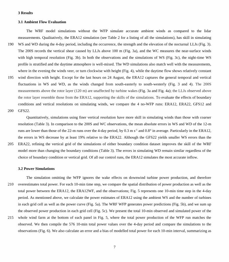
The WRF model simulations without the WFP simulate accurate ambient winds as compared to the lidar

measurements. Qualitatively, the ERA12 simulation (see Table 2 for a listing of all the simulations), has skill in simulating

WS and WD during the 4-day period, including the occurrence, the strength and the elevation of the nocturnal LLJs (Fig. 3). 190

The 200S records the vertical shear caused by LLJs above 100 m (Fig. 3a), and the WC measures the near-surface winds

with high temporal resolution (Fig. 3b). In both the observations and the simulations of WS (Fig. 3c), the night-time WS

profile is stratified and the daytime atmosphere is well-mixed. The WD simulations also match well with the measurements,

where in the evening the winds veer, or turn clockwise with height (Fig. 4), while the daytime flow shows relatively constant

wind direction with height. Except for the last hours on 24 August, the ERA12 captures the general temporal and vertical 195

fluctuations in WS and WD, as the winds changed from south-easterly to south-westerly (Fig. 3 and 4). The 200S

measurements above the rotor layer (120 m) are unaffected by turbine wakes (Fig. 3a and Fig. 4a); the LLJs observed above

the rotor layer resemble those from the ERA12, supporting the skills of the simulations. To evaluate the effects of boundary

conditions and vertical resolutions on simulating winds, we compare the 4 no-WFP runs: ERA12, ERA22, GFS12 and

GFS22. 200

Quantitatively, simulations using finer vertical resolution have more skill in simulating winds than those with coarser

resolution (Table 3). In comparison to the 200S and WC observations, the mean absolute errors in WS and WD of the 12-m

runs are lower than those of the 22-m runs over the 4-day period, by 0.3 m s-1 and 0.8° in average. Particularly in the ERA12,

the errors in WS decrease by at least 19% relative to the ERA22. Although the GFS22 yields smaller WS errors than the

ERA22, refining the vertical grid of the simulations of either boundary condition dataset improves the skill of the WRF 205

model more than changing the boundary conditions (Table 3). The errors in simulating WD remain similar regardless of the

choice of boundary condition or vertical grid. Of all our control runs, the ERA12 simulates the most accurate inflow.

3.2 Power Simulations

The simulation omitting the WFP ignores the wake effects on downwind turbine power production, and therefore

overestimates total power. For each 10-min time step, we compare the spatial distribution of power production as well as the 210

total power between the ERA12, the ERA12WF, and the observations; Fig. 5 represents one 10-min time step in the 4-day

period. As mentioned above, we calculate the power estimates of ERA12 using the ambient WS and the number of turbines

in each grid cell as well as the power curve (Fig. 5a). The WRF WFP generates power predictions (Fig. 5b), and we sum up

the observed power production in each grid cell (Fig. 5c). We present the total 10-min observed and simulated power of the

whole wind farm at the bottom of each panel in Fig. 5, where the total power production of the WFP run matches the 215

observed. We then compile the 576 10-min total power values over the 4-day period and compare the simulations to the

observations (Fig. 6). We also calculate an error and a bias of modelled total power for each 10-min interval, summarizing as

8

the daily root-mean-squared errors (RMSE) and average biases in Table 4 and 5. The large average biases in Table 5

highlight the consistent power overestimation of the no-WFP runs.

Over the 4-day period, the WFP produces total power of the whole wind farm that generally agrees with observation 220

(Fig. 6c). Although the RMSEs between the no-WFP and WFP runs are comparable (Table 4), the average biases are smaller

in the WFP simulations (Table 5). For example, the ERA12WF slightly under-predicts total power by -4.9 MW on average

(Fig. 6c and Table 5). The ERA12, by contrast, consistently over-predicts power production by 41.5 MW (Fig. 6a and Table

5). The daily positive biases of the ERA12 in the first 2 days are nearly 20% of maximum wind farm production (Table 5).

The average positive power bias of 36.2 MW in the ERA22 is also remarkably larger than the mild negative bias of -15.1 225

MW in the ERA22WF (Fig. 6b and d, Table 5). Furthermore, the ERA12 and the GFS12 generally outperform the ERA22

and the GFS22 in power predictions, particularly in RMSE (Fig. 6 and Table 5). However, on the last day, with more south-

westerly flow, the ERA12 and the ERA22 outperform the ERA12WF and the ERA22WF, while the GFS12WF and the

GFS22WF yield smaller errors and biases (Table 4 and 5). Nonetheless, in aggregate, the simulations using the WFP predict

wind-farm power production with more skill than simulations without the WFP. 230

As demonstrated by the average absolute errors (Table 3), the WFP power simulations improve when using 12-m rather

than 22-m vertical resolution (Fig. 6). Changing the vertical grid improves the predictions more than changing boundary

conditions (Table 4 and 5). Particularly in the ERA-interim simulations, the RMSE each day decreases by 19% to 39% when

switching from ERA22WF to ERA12WF, also seen in Fig. 6c and d. Since the power prediction skills of the ERA-interim-

initiated runs and the GFS-initiated runs are comparable, the rest of the paper will focus on the WFP runs using the ERA-235

interim initial and boundary conditions.

Moreover, to statistically differentiate the power productions from various model runs, we apply the 2-sample

Student’s t-test. The null hypothesis of a 2-sample t-test is that the two population means are the same, assuming the

underlying distributions are Gaussian (Wilks, 2011). Hence, if the resultant p-value is equal to or below 0.05, the two

distributions are statically significantly different at the 95% confidence level. For example, the difference between the 4-day 240

power-production averages from the ERA12 and from the ERA12WF is -46.8 MW. The respective p-value is 0, thus the

difference of the means is statistically significant (Table 6). In other words, the ERA12 and the ERA12WF yield different

power production distributions. Similarly, the GFS12 and the GFS12WF lead to statistically different power outputs as the p-

value from t-test is 0 as well (Table 7). We also use the 2-sample t-test to contrast the actual and the modelled power

distributions. For instance, all the p-values between the no-WFP runs and the observation are 0, implying those simulations 245

yield power distributions significantly different from the reality (Table 8).

Given the utility of the WFP, assessing the interactions between atmospheric forcing and power is an important step to

further examine the performance of the WFP. As with the ERA12, the ERA12WF adequately simulates the evolution of the

meteorological variables over the 4-day period (Fig. 7a to d). Both the ERA12 and the ERA12WF capture the overall trends

of hub-height ambient WS and WD measured by the WC (Fig. 7a and b), corresponding to Fig. 3 and 4. On the other hand, 250

although the simulations suggest stronger TKE diurnal cycles than the observations, especially in the first 36 h, the simulated

9

values follow the trends of the WC-measured TKE (Fig. 7c). Although the magnitudes of the surface sensible heat flux of the

surface flux station and the simulations differ, their signs change at similar times, particularly in the last three days (Fig. 7d).

Hence the WRF model is capable to represent diurnal atmospheric stability changes. Note that in Fig. 7c, the lidar derives

TKE using 2-min variances, which is intrinsically different from the modelled TKE, as discussed in Kumer et al. (2016) and 255

Rhodes and Lundquist (2013). Hence, readers should focus on the general trends of the TKE time series, rather than their

absolute values.

The observed WS fluctuates more than the mesoscale simulated WS during daytime (Fig. 7a). The ramp events, where

the WS increases rapidly in a short period (Kamath, 2010; Potter et al., 2009), induce considerable increases in observed

power (Fig. 7e). The five distinct ramp events are from 00 to 01 UTC on 24 August, from 18 to 19 UTC 24 August, from 00 260

to 01 UTC 25 August, from 00 to 02 UTC 26 August, and from 00 to 02 UTC 27 August. Most of the ramp events are

related to the LLJs (Fig. 3), and the simulated WS usually lags that observed (Fig. 7a). Therefore, the WFP under-predicts

total power in nearly all the ramp events (Fig. 7e). Note that the measured WS ranges between the cut-in and rated speed of

the wind turbine, a range in which the power is highly sensitive to WS. The strong linkage between the temporal fluctuations

of WS and power emphasizes the importance of accurate WS predictions. 265

Along the same line, the WFP power performance changes in different meteorological conditions. To quantify WFP’s

skills, we use the bias in total power as a benchmark, calculated by subtracting the observed power from the WFP simulated

power every 10 minutes (Fig. 8). Particularly in conditions of strong winds and weak turbulence, the WFP overestimates

wake effects and thus underestimates power. On the other hand, for calm conditions with moderate or strong turbulence, the

WFP tends to underestimate wake effects and thereby over-predicts power (Fig. 8a and c). The Pearson correlation 270

coefficient between total power bias and WC-observed TKE is 0.48 (not shown).

On the contrary, WD and atmospheric stability have weaker influence on the skill of the WFP in general. The winds

gradually rotate from south-easterly to south-westerly over this 4-day period while maintaining similar magnitudes of wind

speed. During this direction shift, the WFP demonstrates a weak positive power bias when the WD is strictly southerly,

while the biases skew negative when the winds have more easterly or westerly component (Fig. 8b). Similarly, the WFP 275

power bias is unresponsive to stability changes, although strongly stable conditions tend to have low bias (Fig. 8d). Strongly

stable conditions tend to have stronger and more distinct wakes (Abkar and Porté-Agel, 2015b; Lee and Lundquist, 2017;

Magnusson and Smedman, 1994; Rhodes and Lundquist, 2013).

To isolate the WFP errors in power predictions from the WRF model errors in ambient wind simulations, we analyse a

subset of data where the winds are simulated accurately. When the absolute error in wind speed is smaller than 1 m s-1 and 280

the absolute error in wind direction is smaller than 5°, the relationships between power bias and WS, WD and TI (Fig. 9a to

c) remain similar to the general trends shown in Fig. 8a to c. The WS-power-bias and TI-power-bias correlations become

stronger in this subset (Fig 9a and c), compare with all the data in the 4-day period (Fig 8a and c). Moreover, when

considering only cases of accurate wind predictions, the correlation between power bias and stability increases from -0.06

(Fig. 8d) to -0.42 (Fig. 9d). In the few (27) unstable conditions with accurate wind speed predictions, the power bias is 285

10

generally positive, given moderate WS and high TI (Fig 9 a, c and d). In the stable regime, the WFP tends to underestimate

power, regardless of WD (Fig. 9 b and d): 106 of the 125 stable data points are under-predicted. If the few strongest stability

points (z L-1 larger than 0.55) are removed from Fig. 9d, a weak negative correlation with stability emerges as the Pearson

correlation coefficient becomes -0.61. Additionally, generally south to south-westerly flows yield stronger negative power

biases. 290

As may be expected, when the model properly simulates ambient WS, the WFP performs better. When the ERA12WF

predicts larger WS than observed, the simulation over-predicts the total power. The positive WFP power bias corresponds to

WS overestimation, and the negative bias is associated with WS underestimation (Fig. 10). Interestingly, when the error in

simulated total power lies between ±30 MW, the error of the simulated WS is mostly within ±2 m s-1. On the other hand, the

power bias does not seem to be related to wind direction or to ambient TKE: the correlation between the power bias and the 295

simulated WD (TKE) bias is low, 0.3 (0.22) (not shown). Although the simulated WD and TKE generally match the WC

observations (Fig. 7b and c), and the model’s skills in simulating WD and TKE are relatively irrelevant to the WFP’s power

performance.

Although the WFP omits sub-grid-scale wake interactions between the wakes of multiple turbines within a cell, this

omission does not affect the accuracy of the ERA12WF in power prediction: the performance of the WFP is insensitive to 300

the number of turbines per model grid cell. The turbine-normalized bias demonstrates no dependence on the number of

turbines within the model grid cell (Fig. 11). Each whisker in Fig. 11 marks the maximum, the upper quartile, the median,

the lower quartile and the minimum of the average bias. Despite the large positive biases of the maxima, more than half of

the average biases fall between ±1.5 MW, regardless of the numbers of turbines per cell (Fig. 11). Simulating 1 or 4 turbines

in a grid cell (Fig. 1) does not influence the WFP’s overall power prediction performance in the cases shown here. 305

Furthermore, the WFP performance remains consistent between upwind and downwind turbines, based on their

positions against the ambient winds (Fig. 12). Given the square shape of grid cells, we determine the sequential rows of

turbines during strictly southerly flows, with WD between 175° and 185° (Fig. 12a). The bulk of the normalized power

biases fall within 0 to 0.4 MW, regardless of the upwind-downwind positions of turbines. Additionally, the power bias is

independent of the mean distance between the actual turbine locations and the centre points of their respective grid cells (not 310

shown).

4 Discussion

Herein, we compare WRF model simulations with different choices of vertical resolutions and boundary conditions.

The evidence suggests that, at least for this onshore case with a strong diurnal cycle, the vertical resolution is more crucial

than the choice of boundary conditions in simulating accurate winds and wind power production. Shin et al. (2011) have 315

explored the impacts of the lowest model level on the performance of various PBL schemes in the WRF model, suggesting

that increasing the number of model layers can simulate more accurately the surface layer in different stability regimes. In

11

this study, we further illustrate that establishing more vertical levels in the boundary layer as well as the rotor layer improves

the skills of the WRF model in simulating ambient WS, ambient WD and wind power (Table 3, 4 and 5). Furthermore,

Carvalho et al. (2014) discussed the effects of different reanalysis datasets on wind energy production estimates and found 320

the ERA-interim presents the most precise initial and boundary conditions, followed by the GFS. Herein, we test the ERA-

interim and the 0.5° GFS, and both datasets produce simulations that resemble observed winds and power generations. Since

the simulated power is sensitive to the resolution of model vertical grid, particularly near the surface, future WRF WFP users

should select vertical levels with care.

Additionally, the outcomes from the statistical tests among the model runs further validate the importance of using the 325

WFP as well as using a fine vertical grid. From the Student’s t-test, the p-values of all the no-WFP and WFP pairs are 0

(Table 6 and 7), demonstrating that the differences between the distributions of the no-WFP runs and the WFP runs are

statistically significant at any confidence level. Therefore, to accurately simulate power production, applying the WFP is

better than not using it, regardless of the choice of vertical resolution and boundary condition, and the corresponding

improvements in Table 4 and 5 are statistically significant. Although the distinction between the GFS12WF and GFS22WF 330

is not statistically significant at the 90% confidence level (Table 7), switching from ERA22WF to ERA10WF improves

power simulations significantly with 99% confidence (Table 6). In particular, the RMSE drops by 19.1 MW and the bias

reduces by 10.2 MW in average in the ERA12WF (Table 4 and 5), and these are proven statistically significant.

Similarly, results from the statistical tests between the distributions of power from models and observations support the

value of the WFP applied in a fine vertical grid. The p-values of the ERA12WF-observed pair and the GFS12WF-observed 335

pair are 0.106 and 0.167 respectively (Table 8). The high p-values illustrate the distinctions between the distribution of

observed power and the distributions of simulated power from the 12-m WFP simulations are not statistically significant, at

the 90% confidence level. Among all the simulations analysed above, running the WFP over the 12-m vertical grid is the

only combination that is not statistically different from observations (Table 8). In other words, the 12-m WFP simulations

provide the closest approximations, of all the simulations, to the actual power production. Hence, the only way to predict 340

wind-farm power production using the WRF model that is similar to (not statistically different from) observations is to use

the WFP with 12-m resolution, regardless of the boundary condition dataset.

One of the objectives of this study is to propose general directions for improvements on the WFP. First of all, as the

key determining factor in wind power production, WS plays a critical role. Ramp events pose a challenge to the WRF model

in simulating WS as well as to the WFP in predicting power (Fig. 7a and e). On the other hand, wind speeds exceeding 10 m 345

s-1, although below rated speed, lead to WFP power underestimation (Fig. 8a). Furthermore, the WFP performance depends

more on the horizontal winds and turbulence, rather than their vertical components, since the power bias correlates stronger

with TI than TKE (Fig. 8c). Reducing turbulence diffusion in the WRF model could potentially yield more accurate

simulated winds in stable conditions, including LLJs (Sandu et al., 2013); active research in modifying mixing lengths (Jahn

et al., 2017) is suggesting promising results. More importantly, improving the skills of the WRF model in simulating WS can 350

12

improve the WFP power performance (Fig. 10). Future versions of the WRF model as well as the WFP should aim to better

account for instantaneous horizontal WS variations and the subsequent sub-gird wake interactions.

Besides necessary improvements in simulating ambient WS, the WFP scheme itself also requires refinements. When

background winds are accurately predicted, the power-bias dependence on WS and TI remain strong (Fig. 9a and c). The

correlation between the WFP performance and atmospheric stability becomes weakly negative without the strongly stable 355

data (Fig. 9d). Even when the simulated winds are close to observations, the WFP tends to underestimate power during high

WS, low TI and stable conditions. In contrast, the WFP tends to over-predict power in unstable, turbulent conditions, with

the caveat that a small number of unstable cases are considered here. The WFP scheme appears to overestimate wake loss

within a grid cell in stable and windy conditions, and underestimate wake effects in an unstable and well-mixed atmosphere.

Certainly the interactions between WD and wind-farm layout affect the power-bias relationships, while further sensitivity 360

tests can provide more insight into the WFP performance, particularly in intra-cell WS reduction. We demonstrate that inter-

cell wake effects are not the critical factor to power error (Fig. 12b), hence the inability of the WFP to simulate intra-cell

wake effects can explain the biases when many of the turbines experience accurately-simulated ambient flow.

In contrast, WD has no clear influence on the WFP skill (Fig. 8b) in this case, although the irregular shape of the wind

farm adds uncertainty to this relationship. Similarly, the skill of the WFP for this case is insensitive to the number of virtual 365

turbines per cell, and the downwind position of turbines against inflow (Fig. 11 and 12). Compared to the power

overestimation of downwind turbines in the idealized cases described in Vanderwende et al. (2016), both the upwind and

downwind turbine-containing cells presented in this study have consistent positive biases on power production (Fig. 12). Our

findings suggest that the WFP is skilful in simulating power of aggregate wind turbines and can represent the impact of

wakes between grids on power. In the end, the primary limitation of the WFP is rooted in the ambient simulated WS in the 370

WRF model.

5 Conclusion

The WFP scheme in the WRF model (version 3.8.1) provides a convenient way to represent wind farms and their

meteorological impacts in the NWP models. However, its power predictions have not been verified for onshore wind farms

or in a range of wind speed conditions. Herein, we evaluate the performance of the WFP in a range of atmospheric 375

conditions to guide users of the WFP and to suggest future WFP advancements.

Using data from the CWEX-13 campaign, we select a 4-day period, from 24 to 27 August 2013, for our case study, due

to the consistent nocturnal LLJ occurrences. We use measurements from a profiling lidar, a scanning lidar and a surface flux

station to verify the ambient flows simulated by the WRF model. The wind farm of interest, located in central Iowa, consists

of 200 1.5 MW wind turbines. 380

We explore the role of vertical resolution in the operation of the WRF WFP. We evaluate two vertical grids with 12-m

and 22-m resolution near the surface. We find that the finer vertical resolution produces simulations that agree better with

13

observed WS, WD and power than simulations with coarser vertical resolution. Further, because the WFP accounts for the

impacts of wakes on downwind turbine power production, the use of the WFP enables more accurate power prediction,

whereas simulations without the WFP generally over-predict power production. Statically, the WFP simulations with a fine 385

vertical grid, regardless of the boundary conditions, are the most skilful in simulating power.

The skill of the WFP varies with meteorological conditions. When the model simulates WS close to the observations,

the WFP predicts power properly, making WS the critical factor in improving the WFP. Rapid temporal fluctuations in WS

introduce errors in power simulations, especially during ramp events. Further, in windy and less turbulent conditions, the

WFP tends to overestimate wake effects and thus underestimates power production. On the other hand, the WFP 390

performance demonstrates no clear dependence on atmospheric stability, the number of turbines per model grid cell, or the

downwind distance of turbines with respect to the upwind ones.

In conclusion, we demonstrate the value of the WRF WFP and the importance of using a fine vertical grid. Since WS

greatly affects the skill of the WFP, subsequent research could include evaluating the WFP for an even larger range of WS,

especially at wind speeds beyond the turbine cut-out speed (which would be 25 m s-1 in this case; no such high wind speeds 395

were observed during the CWEX-13 campaign). Evaluating the performance of other wind farm layouts and in locations

with complex terrain is also needed. Modifications in the inflow WS considered by the WFP, for example, considering the

rotor equivalent wind speed (REWS) (Wagner et al., 2009), may bring promising improvements. More accurate power

forecasts will shape a more competitive the wind energy industry, and further facilitate grid integration of wind energy

(MacDonald et al., 2016). 400

Data Availability

The code of the WRF-ARW model (doi:10.5065/D6MK6B4K) is publicly available at http://www2.mmm.ucar.edu/wrf/

users/download/get_source.html. This work uses the WRF-ARWmodel and the WRF Pre-Processing System (WPS) version

3.8.1 (released on 12 August, 2016), and the wind farm parameterization is distributed therein. The PSU generic 1.5 MW

turbine (Schmitz, 2012) is available at doi:10.13140/RG.2.2.22492.18567. The user input (namelist) required to run the WRF 405

WFP is available at doi:10.5281/zenodo.847780.

Acknowledgements

This study was funded by the National Science Foundation (Grant number: 1413980; Project Title: CNH-Ex: Legal,

Economic, and Natural Science Analyses of Wind Plant Impacts and Interactions). The CWEX project was supported by the

National Science Foundation under the State of Iowa EPSCoR Grant 1101284. The University of Colorado role in CWEX-410

13 was supported by the National Renewable Energy Laboratory. The authors thank the reviewers and editors for their

thoughtful comments and suggestions. The authors would like to acknowledge high-performance computing support from

14

Yellowstone (ark:/85065/d7wd3xhc) provided by NCAR's Computational and Information Systems Laboratory, sponsored

by the National Science Foundation. The authors would also like to thank NextEra Energy for providing the wind turbine

power data, Iowa State University for providing the surface flux measurements, and NRG Renewable Energy Systems and 415

Leosphere for providing the 200S scanning lidar used in the CWEX-13 campaign.

References

Abkar, M. and Porté-Agel, F.: A new wind-farm parameterization for large-scale atmospheric models, J. Renew. Sustain.

Energy, 7(1), 13121, doi:10.1063/1.4907600, 2015a.

Abkar, M. and Porté-Agel, F.: Influence of atmospheric stability on wind-turbine wakes: A large-eddy simulation study, 420

Phys. Fluids, 27(3), 35104, doi:10.1063/1.4913695, 2015b.

Aitken, M. L., Kosović, B., Mirocha, J. D. and Lundquist, J. K.: Large eddy simulation of wind turbine wake dynamics in

the stable boundary layer using the Weather Research and Forecasting Model, J. Renew. Sustain. Energy, 6(3), 33137,

doi:10.1063/1.4885111, 2014.

Baidya Roy, S.: Simulating impacts of wind farms on local hydrometeorology, J. Wind Eng. Ind. Aerodyn., 99(4), 491–498, 425

doi:10.1016/j.jweia.2010.12.013, 2011.

Barrie, D. B. and Kirk-Davidoff, D. B.: Weather response to a large wind turbine array, Atmos. Chem. Phys., 10(2), 769–

775, doi:10.5194/acp-10-769-2010, 2010.

Bingöl, F., Mann, J. and Foussekis, D.: Conically scanning lidar error in complex terrain, Meteorol. Zeitschrift, 18(2), 189–

195, doi:10.1127/0941-2948/2009/0368, 2009. 430

Blahak, U., Goretzki, B. and Meis, J.: A simple parametrisation of drag forces induced by large wind farms for numerical

weather prediction models, in EWEC, pp. 186–189, Proceedings European Wind Energy Conference and Exhibition., 2010.

Bodini, N., Zardi, D. and Lundquist, J. K.: Three-Dimensional Structure of Wind Turbine Wakes as Measured by Scanning

Lidar, Atmos. Meas. Tech. Discuss., 1–21, doi:10.5194/amt-2017-86, 2017.

Calaf, M., Meneveau, C. and Meyers, J.: Large eddy simulation study of fully developed wind-turbine array boundary layers, 435

Phys. Fluids, 22(1), 15110, doi:10.1063/1.3291077, 2010.

Carvalho, D., Rocha, A., Gómez-Gesteira, M. and Silva Santos, C.: WRF wind simulation and wind energy production

estimates forced by different reanalyses: Comparison with observed data for Portugal, Appl. Energy, 117, 116–126,

doi:10.1016/j.apenergy.2013.12.001, 2014.

Chaboureau, J.-P. and Bechtold, P.: A Simple Cloud Parameterization Derived from Cloud Resolving Model Data: 440

Diagnostic and Prognostic Applications, J. Atmos. Sci., 59(15), 2362–2372, doi:10.1175/1520-

0469(2002)059<2362:ASCPDF>2.0.CO;2, 2002.

Chen, F. and Zhang, Y.: On the coupling strength between the land surface and the atmosphere: From viewpoint of surface

exchange coefficients, Geophys. Res. Lett., 36(10), L10404, doi:10.1029/2009GL037980, 2009.

15

Churchfield, M. J., Lee, S., Michalakes, J. and Moriarty, P. J.: A numerical study of the effects of atmospheric and wake 445

turbulence on wind turbine dynamics, J. Turbul., 13, N14, doi:10.1080/14685248.2012.668191, 2012.

Dee, D. P., Uppala, S. M., Simmons, A. J., Berrisford, P., Poli, P., Kobayashi, S., Andrae, U., Balmaseda, M. A., Balsamo,

G., Bauer, P., Bechtold, P., Beljaars, A. C. M., van de Berg, L., Bidlot, J., Bormann, N., Delsol, C., Dragani, R., Fuentes, M.,

Geer, A. J., Haimberger, L., Healy, S. B., Hersbach, H., Hólm, E. V, Isaksen, L., Kållberg, P., Köhler, M., Matricardi, M.,

McNally, A. P., Monge-Sanz, B. M., Morcrette, J.-J., Park, B.-K., Peubey, C., de Rosnay, P., Tavolato, C., Thépaut, J.-N. 450

and Vitart, F.: The ERA-Interim reanalysis: configuration and performance of the data assimilation system, Q. J. R.

Meteorol. Soc., 137(656), 553–597, doi:10.1002/qj.828, 2011.

Ek, M. B., Mitchell, K. E., Lin, Y., Rogers, E., Grunmann, P., Koren, V., Gayno, G. and Tarpley, J. D.: Implementation of

Noah land surface model advances in the National Centers for Environmental Prediction operational mesoscale Eta model, J.

Geophys. Res., 108(D22), 8851, doi:10.1029/2002JD003296, 2003. 455

Emeis, S.: A simple analytical wind park model considering atmospheric stability, Wind Energy, 13(5), 459–469,

doi:10.1002/we.367, 2010.

Emeis, S. and Frandsen, S.: Reduction of horizontal wind speed in a boundary layer with obstacles, Boundary-Layer

Meteorol., 64(3), 297–305, doi:10.1007/BF00708968, 1993.

Eriksson, O., Lindvall, J., Breton, S.-P. and Ivanell, S.: Wake downstream of the Lillgrund wind farm - A Comparison 460

between LES using the actuator disc method and a Wind farm Parametrization in WRF, J. Phys. Conf. Ser., 625(1), 12028,

doi:10.1088/1742-6596/625/1/012028, 2015.

Fitch, A. C.: Notes on using the mesoscale wind farm parameterization of Fitch et al. (2012) in WRF, Wind Energy, 19,

1757–1758, doi:10.1002/we.1945, 2015.

Fitch, A. C., Olson, J. B., Lundquist, J. K., Dudhia, J., Gupta, A. K., Michalakes, J. and Barstad, I.: Local and Mesoscale 465

Impacts of Wind Farms as Parameterized in a Mesoscale NWP Model, Mon. Weather Rev., 140(9), 3017–3038,

doi:10.1175/MWR-D-11-00352.1, 2012.

Fitch, A. C., Lundquist, J. K. and Olson, J. B.: Mesoscale Influences of Wind Farms throughout a Diurnal Cycle, Mon.

Weather Rev., 141(7), 2173–2198, doi:10.1175/MWR-D-12-00185.1, 2013a.

Fitch, A. C., Olson, J. B. and Lundquist, J. K.: Parameterization of Wind Farms in Climate Models, J. Clim., 26(17), 6439–470

6458, doi:10.1175/JCLI-D-12-00376.1, 2013b.

Frandsen, S. T., Jørgensen, H. E., Barthelmie, R., Rathmann, O., Badger, J., Hansen, K., Ott, S., Rethore, P.-E., Larsen, S. E.

and Jensen, L. E.: The making of a second-generation wind farm efficiency model complex, Wind Energy, 12(5), 445–458,

doi:10.1002/we.351, 2009.

Iacono, M. J., Delamere, J. S., Mlawer, E. J., Shephard, M. W., Clough, S. A. and Collins, W. D.: Radiative forcing by long-475

lived greenhouse gases: Calculations with the AER radiative transfer models, J. Geophys. Res. Atmos., 113(D13), D13103,

doi:10.1029/2008JD009944, 2008.

Ito, J., Niino, H., Nakanishi, M. and Moeng, C.-H.: An Extension of the Mellor–Yamada Model to the Terra Incognita Zone

16

for Dry Convective Mixed Layers in the Free Convection Regime, Boundary-Layer Meteorol., 157(1), 23–43,

doi:10.1007/s10546-015-0045-5, 2015. 480

Jahn, D. E., Takle, E. S. and Gallus, W. A.: Improving Wind-Ramp Forecasts in the Stable Boundary Layer, Boundary-

Layer Meteorol., 163, 423–446, doi:10.1007/s10546-017-0237-2, 2017.

Jimenez, A., Crespo, A., Migoya, E. and Garcia, J.: Advances in large-eddy simulation of a wind turbine wake, J. Phys.

Conf. Ser., 75(1), 12041, doi:10.1088/1742-6596/75/1/012041, 2007.

Jiménez, P. A., Navarro, J., Palomares, A. M. and Dudhia, J.: Mesoscale modeling of offshore wind turbine wakes at the 485

wind farm resolving scale: a composite-based analysis with the Weather Research and Forecasting model over Horns Rev,

Wind Energy, 18(3), 559–566, doi:10.1002/we.1708, 2015.

Kain, J. S.: The Kain–Fritsch Convective Parameterization: An Update, J. Appl. Meteorol., 43(1), 170–181,

doi:10.1175/1520-0450(2004)043<0170:TKCPAU>2.0.CO;2, 2004.

Kamath, C.: Understanding wind ramp events through analysis of historical data, in IEEE PES T&D 2010, pp. 1–6, IEEE., 490

2010.

Keith, D. W., DeCarolis, J. F., Denkenberger, D. C., Lenschow, D. H., Malyshev, S. L., Pacala, S. and Rasch, P. J.: The

influence of large-scale wind power on global climate, Proc. Natl. Acad. Sci. U. S. A., 101(46), 16115–16120,

doi:10.1073/pnas.0406930101, 2004.

Kumer, V.-M., Reuder, J., Dorninger, M., Zauner, R. and Grubišić, V.: Turbulent kinetic energy estimates from profiling 495

wind LiDAR measurements and their potential for wind energy applications, Renew. Energy, 99, 898–910,

doi:10.1016/j.renene.2016.07.014, 2016.

Lee, J. C. Y. and Lundquist, J. K.: Observing and Simulating Wind-Turbine Wakes During the Evening Transition,

Boundary-Layer Meteorol., 164(3), 449–474, doi:10.1007/s10546-017-0257-y, 2017.

Lundquist, J. K., Takle, E. S., Boquet, M., Kosović, B., Rhodes, M. E., Rajewski, D., Doorenbos, R., Irvin, S., Aitken, M. L. , 500

Friedrich, K., Quelet, P. T., Rana, J., Martin, C. S., Vanderwende, B. and Worsnop, R.: Lidar observations of interacting

wind turbine wakes in an onshore wind farm, in EWEA. [online] Available from: http://www.leosphere.com/wp-

content/uploads/2014/03/Lundquist_Boquet_EWEA_2014_CWEX13_final.pdf (Accessed 10 May 2017), 2014.

Lundquist, J. K., Churchfield, M. J., Lee, S. and Clifton, A.: Quantifying error of lidar and sodar Doppler beam swinging

measurements of wind turbine wakes using computational fluid dynamics, Atmos. Meas. Tech., 8(2), 907–920, 505

doi:10.5194/amt-8-907-2015, 2015.

MacDonald, A. E., Clack, C. T. M., Alexander, A., Dunbar, A., Wilczak, J. and Xie, Y.: Future cost-competitive electricity

systems and their impact on US CO2 emissions, Nat. Clim. Chang., 6(5), 526–531, doi:10.1038/nclimate2921, 2016.

Magnusson, M. and Smedman, A. S.: Influence of atmospheric stability on wind turbine wakes, Wind Eng., 18(3), 139–152,

1994. 510

Marquis, M., Wilczak, J., Ahlstrom, M., Sharp, J., Stern, A., Smith, J. C. and Calvert, S.: Forecasting the Wind to Reach

Significant Penetration Levels of Wind Energy, Bull. Am. Meteorol. Soc., 92(9), 1159–1171,

17

doi:10.1175/2011BAMS3033.1, 2011.

Miller, L. M., Brunsell, N. A., Mechem, D. B., Gans, F., Monaghan, A. J., Vautard, R., Keith, D. W. and Kleidon, A.: Two

methods for estimating limits to large-scale wind power generation, Proc. Natl. Acad. Sci., 112(36), 11169–11174, 515

doi:10.1073/pnas.1408251112, 2015.

Mirocha, J. D., Kosovic, B., Aitken, M. L. and Lundquist, J. K.: Implementation of a generalized actuator disk wind turbine

model into the weather research and forecasting model for large-eddy simulation applications, J. Renew. Sustain. Energy,

6(1), 13104, doi:10.1063/1.4861061, 2014.

Mirocha, J. D., Rajewski, D. A., Marjanovic, N., Lundquist, J. K., Kosović, B., Draxl, C. and Churchfield, M. J.: 520

Investigating wind turbine impacts on near-wake flow using profiling lidar data and large-eddy simulations with an actuator

disk model, J. Renew. Sustain. Energy, 7(4), 43143, doi:10.1063/1.4928873, 2015.

Muñoz-Esparza, D., Lundquist, J. K., Sauer, J. A., Kosović, B. and Linn, R. R.: Coupled mesoscale-LES modeling of a

diurnal cycle during the CWEX-13 field campaign: From weather to boundary-layer eddies, J. Adv. Model. Earth Syst.,

doi:10.1002/2017MS000960, 2017. 525

Na, J. S., Koo, E., Muñoz-Esparza, D., Jin, E. K., Linn, R. and Lee, J. S.: Turbulent kinetics of a large wind farm and their

impact in the neutral boundary layer, Energy, 95, 79–90, doi:10.1016/j.energy.2015.11.040, 2016.

Nakanishi, M. and Niino, H.: An Improved Mellor–Yamada Level-3 Model: Its Numerical Stability and Application to a

Regional Prediction of Advection Fog, Boundary-Layer Meteorol., 119(2), 397–407, doi:10.1007/s10546-005-9030-8, 2006.

Potter, C. W., Grimit, E. and Nijssen, B.: Potential benefits of a dedicated probabilistic rapid ramp event forecast tool, in 530

2009 IEEE/PES Power Systems Conference and Exposition, pp. 1–5, IEEE., 2009.

Rajewski, D. A., Takle, E. S., Lundquist, J. K., Oncley, S., Prueger, J. H., Horst, T. W., Rhodes, M. E., Pfeiffer, R., Hatfield,

J. L., Spoth, K. K. and Doorenbos, R. K.: Crop Wind Energy Experiment (CWEX): Observations of Surface-Layer,

Boundary Layer, and Mesoscale Interactions with a Wind Farm, Bull. Am. Meteorol. Soc., 94(5), 655–672,

doi:10.1175/BAMS-D-11-00240.1, 2013. 535

Rajewski, D. A., Takle, E. S., Lundquist, J. K., Prueger, J. H., Pfeiffer, R. L., Hatfield, J. L., Spoth, K. K. and Doorenbos, R.

K.: Changes in fluxes of heat, H2O, and CO2 caused by a large wind farm, Agric. For. Meteorol., 194, 175–187,

doi:10.1016/j.agrformet.2014.03.023, 2014.

Rajewski, D. A., Takle, E. S., Prueger, J. H. and Doorenbos, R. K.: Toward understanding the physical link between turbines

and microclimate impacts from in situ measurements in a large wind farm, J. Geophys. Res. Atmos., 121(22), 540

2016JD025297, doi:10.1002/2016JD025297, 2016.

Rhodes, M. E. and Lundquist, J. K.: The Effect of Wind-Turbine Wakes on Summertime US Midwest Atmospheric Wind

Profiles as Observed with Ground-Based Doppler Lidar, Boundary-Layer Meteorol., 149(1), 85–103, doi:10.1007/s10546-

013-9834-x, 2013.

Sandu, I., Beljaars, A., Bechtold, P., Mauritsen, T. and Balsamo, G.: Why is it so difficult to represent stably stratified 545

conditions in numerical weather prediction (NWP) models?, J. Adv. Model. Earth Syst., 5(2), 117–133,

18

doi:10.1002/jame.20013, 2013.

Schmitz, S.: XTurb-PSU: A Wind Turbine Design and Analysis Tool, [online] Available from:

http://www.aero.psu.edu/Faculty_Staff/schmitz/XTurb/XTurb.html, 2012.

Sharma, V., Calaf, M., Lehning, M. and Parlange, M. B.: Time-adaptive wind turbine model for an LES framework, Wind 550

Energy, 19(5), 939–952, doi:10.1002/we.1877, 2016.

Shin, H. H., Hong, S.-Y. and Dudhia, J.: Impacts of the Lowest Model Level Height on the Performance of Planetary

Boundary Layer Parameterizations, Mon. Weather Rev., 140(2), 664–682, doi:10.1175/MWR-D-11-00027.1, 2011.

Skamarock, W. C. and Klemp, J. B.: A time-split nonhydrostatic atmospheric model for weather research and forecasting

applications, J. Comput. Phys., 227(7), 3465–3485, doi:10.1016/j.jcp.2007.01.037, 2008. 555

Stull, R. B.: An Introduction to Boundary Layer Meteorology, Springer., 1988.

Thompson, G. and Eidhammer, T.: A Study of Aerosol Impacts on Clouds and Precipitation Development in a Large Winter

Cyclone, J. Atmos. Sci., 71(10), 3636–3658, doi:10.1175/JAS-D-13-0305.1, 2014.

Vanderwende, B. and Lundquist, J. K.: Could Crop Height Affect the Wind Resource at Agriculturally Productive Wind

Farm Sites?, Boundary-Layer Meteorol., 158(3), 409–428, doi:10.1007/s10546-015-0102-0, 2016. 560

Vanderwende, B. J., Lundquist, J. K., Rhodes, M. E., Takle, E. S. and Irvin, S. L.: Observing and Simulating the

Summertime Low-Level Jet in Central Iowa, Mon. Weather Rev., 143(6), 2319–2336, doi:10.1175/MWR-D-14-00325.1,

2015.

Vanderwende, B. J., Kosović, B., Lundquist, J. K. and Mirocha, J. D.: Simulating effects of a wind turbine array using LES

and RANS, J. Adv. Model. Earth Syst., 8(3), 1376–1390, doi:10.1002/2016MS000652, 2016. 565

Vautard, R., Thais, F., Tobin, I., Bréon, F.-M., Lavergne, J.-G. D. de, Colette, A., Yiou, P. and Ruti, P. M.: Regional climate

model simulations indicate limited climatic impacts by operational and planned European wind farms, Nat. Commun., 5,

doi:10.1038/ncomms4196, 2014.

Volker, P. J. H., Badger, J., Hahmann, A. N. and Ott, S.: The Explicit Wake Parametrisation V1.0: a wind farm

parametrisation in the mesoscale model WRF, Geosci. Model Dev., 8(11), 3715–3731, doi:10.5194/gmd-8-3715-2015, 2015. 570

Wagner, R., Antoniou, I., Pedersen, S. M., Courtney, M. S. and Jørgensen, H. E.: The influence of the wind speed profile on

wind turbine performance measurements, Wind Energy, 12(4), 348–362, doi:10.1002/we.297, 2009.

Wilczak, J., Finley, C., Freedman, J., Cline, J., Bianco, L., Olson, J., Djalalova, I., Sheridan, L., Ahlstrom, M., Manobianco,

J., Zack, J., Carley, J. R., Benjamin, S., Coulter, R., Berg, L. K., Mirocha, J., Clawson, K., Natenberg, E. and Marquis, M.:

The Wind Forecast Improvement Project (WFIP): A Public–Private Partnership Addressing Wind Energy Forecast Needs, 575

Bull. Am. Meteorol. Soc., 96(10), 1699–1718, doi:10.1175/BAMS-D-14-00107.1, 2015.

Wilczak, J. M., Oncley, S. P. and Stage, S. A.: Sonic Anemometer Tilt Correction Algorithms, Boundary-Layer Meteorol.,

99(1), 127–150, doi:10.1023/A:1018966204465, 2001.

Wilks, D. S.: Statistical methods in the atmospheric sciences, Academic Press., 2011.

WRF-ARW: WRF Model Version 3.8: Updates, , doi:doi:10.5065/D6MK6B4K, 2016. 580

19

Wu, Y.-T. and Porté-Agel, F.: Large-Eddy Simulation of Wind-Turbine Wakes: Evaluation of Turbine Parametrisations,

Boundary-Layer Meteorol., 138(3), 345–366, doi:10.1007/s10546-010-9569-x, 2011.

585

20

Figure 1: Map of the 3 domains (d01, d02 and d03) in the WRF simulations (right), with the white x representing the CWEX-13

wind farm. Zoom-in map of the wind farm (left), with the black horizontal and vertical lines outlining the WRF grid cells, the red

dots as the actual locations of wind turbines, the blue numbers as the number of wind turbines per WRF grid cell, the yellow

square as the WC lidar, the green square as the 200S lidar and the purple square as the surface flux station. Other instruments 590 were deployed in CWEX-13, and only the instruments used herein are shown.

21

Figure 2: Illustration of the two vertical grids chosen: 12 m on the left in blue and 22 m on the right in red. Both grids shown use

the ERA-interim as the boundary conditions. The simulations initiated with the 0.5° GFS have slightly different grids.

595

22

Figure 3: Time-height contour of WS from the 200S (a), the WC (b) and ERA12 at the closest grid point to the 200S (c).

23

Figure 4: As in Fig. 3, but for WD. 600

24

Figure 5: The power production for one 10-min period from the ERA12 estimates (a), the ERA12WF outputs (b) and the

observation (abbreviated as OBS) (c). The total power in each grid cell is presented regardless of the number of turbines in each

cell, and the wind-farm totals are summarized at the bottom. The vectors indicate the simulated winds, and their lengths

correspond to the horizontal velocity magnitude. 605

25

Figure 6: Scatter plots comparing the 10-min average observed total power against the calculated total power from the ERA12 (a)

and the ERA22 (b), and the simulated total power from the ERA12WF (c) and the ERA22WF (d). The dots represent the total

power on 24 August (purple), 25 August (blue), 26 August (green) and 27 August (yellow). 610

26

Figure 7: Time series of hub-height WS (a), hub-height WD (b), hub-height TKE (c), surface sensible heat flux (d), and total wind

farm power (e) from the measurements (in red) and the simulations (ERA12WF, in black; ERA12, in blue). The simulated values

are interpolated to hub height at the grid point closest to the WC location. In (b), the grey horizontal dash line marks the WD of 615 180°. In (d), the grey horizontal dash line marks the heat flux of 0 W m-2.

27

Figure 8: Scatter plots comparing the bias of the ERA12WF 10-min total power to the WC-observed hub-height WS (a), hub-

height WD (b), hub-height TI (c) and stability parameter z L-1 measured at the surface flux station (d). The r represents the

Pearson correlation coefficient. Similar to Fig. 6, different coloured dots represent biases on different days. The horizontal black 620 dash lines mark the zero power bias, and the vertical black dash line in (d) at zero z L-1 differentiates the two stability regimes.

28

Figure 9: As in Fig. 8, and only including data when the winds are accurately simulated in the ERA12WF run: the modelled-

observed absolute error in WS smaller than 1 m s-1 and the absolute error in WD smaller than 5°. Different colours represent

different WD bins: 150° to 170° in blue, 170° to 190° in cyan, 190° to 210° in orange, 210° to 230° in red, and 230° and beyond in 625 maroon. The n values illustrate the respective sample size in each wind-direction bin. Solid circles represent unstable conditions (z

L-1 smaller than 0) and hollow circles represent stable conditions (z L-1 larger than 0).

29

Figure 10: Scatter plot between the bias of the ERA12WF 10-min total power compared to observation, and its bias of the 630 simulated hub-height WS in the closest grid cell to the WC. The r represents the Pearson correlation coefficient.

30

Figure 11: Boxplot of the average bias of the ERA12WF simulated power across different numbers of wind turbine per WRF grid

cell every 10 minutes during the 4-day period. 635

31

Figure 12: Map of the wind farm where the blue numbers represent the row number from the upwind row during southerly winds

(a). The upwind row number is reset to 1 when the next two downwind grid boxes to the North contain no turbines. Boxplot of the

average ERA12WF power bias normalized over different number of wind turbine rows, when the hub-height WD in the grid cell 640 closest to the WC is between 175° and 185° (b).

32

Table 1: The WRF model configuration.

Parameterization Scheme Reference

Cumulus Kain-Fritsch Kain (2004)

Land surface NOAH LSM Ek et al. (2003)

Land surface roughness Thermal roughness length Chen and Zhang (2009)

Microphysics Thompson aerosol-aware Thompson and Eidhammer (2014)

PBL MYNN Level 2.5 Nakanishi and Niino (2006)

Radiation RRTMG Iacono et al. (2008)

645

Table 2: List of WRF simulations and their features.

Run name Boundary condition Vertical resolution WFP

ERA12 ERA-interim 12 m No

ERA22 ERA-interim 22 m No

GFS12 0.5° GFS 12 m No

GFS22 0.5° GFS 22 m No

ERA12WF ERA-interim 12 m Yes

ERA22WF ERA-interim 22 m Yes

GFS12WF 0.5° GFS 12 m Yes

GFS22WF 0.5° GFS 22 m Yes

33

Table 3: Average absolute error in WS (m s-1) and WD (°) of different no-WFP runs.

ERA12 ERA22 GFS12 GFS22

200S 120 m WS 1.49 1.84 1.35 1.54

WC 120 m WS 1.21 1.63 1.34 1.48

WC 80 m WS 1.24 1.64 1.36 1.55

WC 40 m WS 1.47 1.9 1.53 1.86

200S 120 m WD 14.99 15.98 14.68 14.99

WC 120 m WD 12.66 13.86 13.07 13.47

WC 80 m WD 13.23 14.55 13.85 14.24

WC 40 m WD 14.19 15.58 14.83 15.15

650

The smallest errors across different WRF settings are highlighted in bold.

34

Table 4: RMSE of 10-min total power (MW) of different model runs each day.

24 Aug 25 Aug 26 Aug 27 Aug 4-day mean

ERA12 73.6 73.5 35.4 22.6 51.3

ERA22 79.5 72.8 48.5 41 60.5

GFS12 62 76.5 58.3 40.9 59.4

GFS22 73.9 89.6 65.3 51.9 70.2

ERA12WF 42.2 49.4 31.1 46.5 42.3

ERA22WF 61.7 61.2 50.9 71.6 61.4

GFS12WF 46.2 54.6 34.1 36.1 42.8

GFS22WF 40 60 32.6 37.3 42.5

655

Table 5: Average bias of 10-min total power (MW) of different model runs each day.

24 Aug 25 Aug 26 Aug 27 Aug 4-day mean

ERA12 68.3 62.6 26.8 8.1 41.5

ERA22 58.3 52.1 28 6.2 36.2

GFS12 49.4 65 51.8 29 48.8

GFS22 65.5 80.7 60.3 35.8 60.6

ERA12WF 17.5 16.6 -12.2 -41.6 -4.9

ERA22WF 10.4 0.6 -17.6 -53.6 -15.1

GFS12WF 3.8 22.2 9.6 -18.6 4.3

GFS22WF 2.9 29.7 10.9 -12.3 7.8

The RMSEs and biases closest to zero across different days are highlighted in bold.

660

35

Table 6: Differences (first value) and p-values (second value) from 2-sample t-tests of simulated power from different ERA runs.

ERA12 ERA12WF ERA22WF

4-day mean 41.8 -4.9 -15.1

ERA12 41.9 -46.8; 0

ERA22 36.1 5.7; 0.0300 -51.2; 0

ERA12WF -4.9

ERA22WF -15.1 10.2; 9.60×10-4

Table 7: As in Table 6, but for GFS runs.

GFS12 GFS12WF GFS22WF

4-day mean 48.6 4.2 7.8

GFS12 48.6 -44.4; 0

GFS22 60.6 -12.0; 1.09×10-7 -52.8; 0

GFS12WF 4.2

GFS22WF 7.8 -3.6; 0.163

Table 8: P-values from 2-sample t-tests of the 10-min observed power and the 10-min simulated power from different model runs. 665

Simulated 4-day mean Observed 4-day mean Difference of means P-value

ERA12 212.7

170.9

41.8 0

ERA22 207.0 36.1 0

GFS12 219.5 48.6 0

GFS22 231.4 60.5 0

ERA12WF 166.0 -4.9 0.106

ERA22WF 155.8 -15.1 6.54×10-6

GFS12WF 175.1 4.2 0.167

GFS22WF 178.7 7.8 0.0136