Embed Size (px)
Citation preview

Scientia Iranica A (2016) 23(1), 142{154
Sharif University of TechnologyScientia Iranica
Transactions A: Civil Engineeringwww.scientiairanica.com
Evaluation of the static and seismic active lateral earthpressure for c� � soils by the ZEL method
A. Keshavarz� and Z. Pooresmaeil
School of Engineering, Persian Gulf University, Bushehr, Iran.
Received 9 November 2014; received in revised form 11 April 2015; accepted 2 June 2015
KEYWORDSZero extension lines;Static;Seismic;Active;Lateral earth pressure;Retaining walls;Non-associated.
Abstract. The method of Zero Extension Lines (ZEL) has been used to evaluate thestatic and seismic active lateral earth pressure on an inclined wall retaining c� � back�ll.The equilibrium equations along the zero extension lines have been solved using the �nitedi�erence method. A computer code is prepared to analyze the retaining wall, calculate theZEL network and the distribution of the active lateral earth pressure behind the retainingwall. The total active force on the retaining wall was de�ned as the lateral earth pressurecoe�cients due to the soil unit weight, the surcharge, and the soil cohesion. The variationsof the active lateral earth pressure coe�cients with changes in di�erent parameters, suchas the inclination of the earth and wall, the friction angle of the soil, the adhesion of thesoil-wall interface, the horizontal and vertical pseudo-static earthquake coe�cients, havebeen obtained. The results have been obtained for soils with associated and non-associated ow rules. The e�ect of the dilation angle has also been considered. The results obtainedin this study are very close to those of other methods and con�rm that the ZEL methodcan be successfully used to evaluate the lateral earth pressure of retaining walls.© 2016 Sharif University of Technology. All rights reserved.
1. Introduction
Many di�erent methods are provided to evaluate theactive lateral earth pressure on the retaining wall.Rankin and Coulomb are the common methods. Stresscharacteristics [1,2] or slip lines method, limit analysismethod [3,4], Rankine's conjugate stress concept [5],and slice analysis method [6] are also used to evaluatethe lateral earth pressure. Zero Extension Lines(ZEL) method is one of the methods that is capableof analyzing the stability of retaining walls undergeneral conditions in static and seismic conditions.This method was �rst used by Roscoe [7] to solvestatic and dynamic problems of retaining walls. In1971, James and Bransby [8] used ZEL method to
*. Corresponding author. Tel/Fax: +98 77 33440376E-mail addresses: [email protected]; andamin [email protected] (A. Keshavarz);[email protected] (Z. Pooresmaeil)
predict the strain patterns behind retaining walls.Habibagahi and Ghahramani [9] presented an earthpressure theory based on the simple ZEL �eld to predictstress patterns in the back�ll behind a vertical wall.Anvar and Ghahramani [10] derived the equilibriumequations along the ZEL and presented the applicationof ZEL method. Jahanandish [11] developed a theoryregarding the ZEL method and derived the equilibriumequations along zero extension lines for axial symmetry.Furthermore, ZEL method has also been used to studythe stability of slopes [12], analyze three-dimensionalstability of soils [13], predict the behavior of densefrictional soils [14], and evaluate bearing capacity ofsoils and foundations and dynamic lateral pressure ofretaining structures [15-17]. Veiskarami et al. [18-20]used this method to predict the bearing capacity offoundations and load-displacement behavior of shallowfoundations considering the stress level e�ect.
Many available methods evaluate lateral earthpressure on the retaining walls by using the assumption

A. Keshavarz and Z. Pooresmaeil/Scientia Iranica, Transactions A: Civil Engineering 23 (2016) 142{154 143
of the associated ow rule, although `Real' soils havea non-associated ow rule and the dilation angle issmaller than the friction angle [21]. One of theadvantages of ZEL method is that in this method, soilcan be associative or non-associative. Therefore, byusing the ZEL method, the e�ect of the dilation anglecan be evaluated. Lee and Herington [22] evaluatedthe passive earth pressures for non-associated ow rulesby a theoretical study. Shiau and Smith [23] studied,numerically, the e�ect of non-associated ow rule onthe passive earth pressure. Benmeddour et al. [21]provided passive and active lateral earth pressurecoe�cients due to the soil unit weight for the soilwith dilation angle equal to zero. They studied thein uence of non-associativity by a numerical methodand modifying values of the soil friction angle andcohesion.
Moreover, ZEL method does not have the limita-tion of assuming the shape of the rupture surface. Byusing this method, the failure zone is determined afteranalyzing the retaining wall. ZEL method analyzesgeotechnical problems in the strain �eld. When thesoil is assumed as associative soil, i.e. the friction angleof the soil is equal to its dilation angle, ZEL method issimilar to the stress characteristics or slip lines method.
The ZEL method has been used in this paper toevaluate the seismic stability of retaining walls for non-associated and associated ow rules and propose thelateral earth pressure coe�cients. Although Habiba-gahi and Ghahramani [9] developed the ZEL for staticlateral earth pressure, they used the simple ZEL �ledand developed the method for sands. This studydevelops the ZEL method for the active lateral earthpressure for c � � soils in seismic case. Considerationof the e�ect of di�erent parameters of the soil andretaining wall, especially the soil dilation angle, isone of the advantages of this study. Also, the lateralearth pressure coe�cients due to the soil unit weight,surcharge, and soil cohesion have been provided fornon-associative soil.
2. Theory
The geometry of the retaining wall in the active casehas been shown in Figure 1(a). The surcharge q isapplied on the ground surface. The ground surfacemakes an angle � with the horizontal direction and thewall angle with the vertical direction is �. The heightof the retaining wall is H. The positive directions ofthe � and � are shown in Figure 1(a).
2.1. Assumptions1. The back�ll soil is considered as a c � � soil and
follows the Mohr-Coulomb yield criterion, where cis the cohesion in kPa and � is the internal frictionangle in degree;
2. The unit weight of the soil mass is assumed equalto in kN/m3;
3. The friction angle in the interface between soil andwall is considered as �w in degree;
4. The adhesion of the soil-wall interface is assumedcw in kPa;
5. The principle of superposition is valid for static andseismic analyses;
6. The retaining wall problem is considered planestrain and two dimensional.
2.2. Boundary conditionsAnalyzing the problem requires knowing the boundaryconditions along the ground surface and the retainingwall. The boundary conditions are explained in thefollowing sections.
2.2.1. Along the ground surfaceTo calculate the coordinates (x; z) of the points onthe ground surface, a length of L is considered on thisboundary and it is divided into n divisions. Accordingto Figure 1(a), the coordinates of the point number ion the ground surface can be calculated as:
xi = �Ln
(i� 1) cos�; zi = xi tan�; (1)
where � is the ground angle with horizontal direction.As mentioned before, the vertical stress q is applied onthe ground surface. So, the normal and shear stressesfor the points on the ground are obtained as:�0 = q cos� [(1� kv) cos� � kh sin�] ;
�0 = q cos� [(1� kv) sin� + kh cos�] ; (2)
where kh and kv are horizontal and vertical pseudo-static earthquake coe�cients.
The Mohr circle of stress on the ground can beshown in Figure 1(b). The average stress on the ground(p0) is obtained from the Mohr circle:
p0 =
�0+c cos� sin��q
(�0 sin�+c cos�)2�(�0 cos�)2
cos2 �:
(3)
Using the Mohr circle of stress, the angle (the anglebetween "1 and the horizontal axis) on the groundsurface ( 0) can also be calculated as:
if q = 0 : 0 = � +�2
else 0 =�2
+ 0:5���� � sin�1
�p0 sin(�+�)
R0
��;(4)
where:
tan � =kh
1� kv ; R0 = p0 sin�+ c cos�: (5)

144 A. Keshavarz and Z. Pooresmaeil/Scientia Iranica, Transactions A: Civil Engineering 23 (2016) 142{154
Figure 1. The retaining wall problem: (a) Geometry and ZEL network; (b) boundary condition along the ground surface;and (c) boundary condition along the retaining wall.
2.2.2. Along the retaining wallAssuming the normal and shear stresses on the retain-ing wall, the Mohr circle of stress on this boundaryis shown in Figure 1(c). The following equations arederived from this �gure:
f =�2
+ � + �;
�f = pf �Rf cos 2�f ;
�f = cw + �f tan �w; (6)
where �f and �f are the normal and shear stresses onthe retaining wall, respectively. Then, the angle onthe wall ( f ) can be calculated from Eq. (6):
f =�2
+ �
+0:5���w+sin�1
�pf sin �w+cw cos �wpf sin�+cos�
��: (7)
2.3. Equilibrium equations along the zeroextension lines
By considering the soil shearing in a principal plane forplane strain problem, major and minor principal strainincrements do not have the same concept. Therefore,two lines (AP and BP) in the soil element will havethe linear strains equal to zero in their directions(Figure 2). AP and BP are called the zero extensionlines in minus direction (ZEL�) and plus direction(ZEL+), respectively.
Each point in the soil has four features, x, z,p, and . By solving the equations along the zeroextension lines, these features can be determined. Asillustrated in Figure 2, the angle between zero extensionlines is �=2�v, where v is the dilation angle of the soil.The angle of zero extension lines with x axis is � �.Angle � is de�ned as follows:
� =�4� v
2: (8)
Therefore, the slope of these lines is expressed as:

A. Keshavarz and Z. Pooresmaeil/Scientia Iranica, Transactions A: Civil Engineering 23 (2016) 142{154 145
Figure 2. The directions of zero extension lines and Mohr circle of the strain [10].
Plus ZEL, PB :dzdx
= tan( + �); (9)
Minus ZEL, PB :dzdx
= tan( � �): (10)
The equilibrium equations along the plus and minuszero extension lines can be written as [10]:
dp+ 2(p tan�+ c)�
��d + ��@ @"� d"
+�
= fx �� (��dx� tan�dz) + fz �� (tan�dx+ ��dz) ;(11)
and along the plus ZEL:
dp� 2(p tan�+ c)�
��d + ��@ @"+ d"
��
= fx �� (��dx� tan�dz) + fz �� (tan�dx+ ��dz) ;(12)
where fx and fz are body forces along the x and z axeswhich are de�ned as � kh and � (1 � kv); d"+ andd"� are the length of the plus and minus zero extensionlines, respectively, and:
�� =1� sin v sin�
cos v cos�;
�� =cos vcos�
;
�� =sin�� sin vcos� cos v
: (13)
If x, z, p, and of points A and B are known, thesevalues of any point P can be found by writing Eqs. (9)-(12) in the �nite di�erence form:
xP =ZA � ZB � xAtgmm+ xBtgmp
tgmp� tgmm ; (14)
zP = (xC � xB) tgmp+ zB ; (15)
pP = pB +A1 �Bmp( C � B); (16)
P =A3
A4: (17)
The parameters in Eqs. (14)-(17) are de�ned in theappendix. By using the trial-and-error procedure,a function is written in MATLAB to calculate theunknown parameters (x, z, p, and ) of point P .First, it is assumed that these parameters are equalto the parameters of points A and B on the minus andplus ZEL, respectively. Then, the new parameters ofpoint P can be calculated using Eqs. (14)-(17). Thisprocedure is repeated until the di�erence between thenew and old parameters of point P is small enough.
2.4. ZEL networksA computer code in MATLAB is provided to analyzethe problem. The code starts the calculation fromthe ground surface. The calculation continues todetermine the characteristics of the points on theretaining wall. Three di�erent types of ZEL networkcan arise according to the magnitudes of 0 and f(Figure 3).
Type 1, f = 0: In this case, the ZEL networkincludes Rankin and mixed zones. First, the points inRankin zone are solved by using the boundary condi-tions on the ground surface and equilibrium equationsalong the ZEL lines. Then, the network in the mixedzone is determined knowing the information on lineOA2 and the boundary conditions along the retainingwall.
Type 2, f > 0: In this case, the ZEL networkincludes three zones: Rankin, Goursat, and mixed.

146 A. Keshavarz and Z. Pooresmaeil/Scientia Iranica, Transactions A: Civil Engineering 23 (2016) 142{154
Figure 3. Di�erent types of ZEL networks.
Figure 4. The soil element on the stress discontinuity line and Mohr circle.
First, the points in Rankin zone are solved by usingthe boundary conditions on the ground surface andequilibrium equations along the ZEL lines. Now, therelation between and p should be obtained to solvethe points in Goursat zone. The p and in the leftand right of point O (Figure 1) are di�erent and asingularity exists at this point.
Therefore, at point O, dx = dz = 0, and therelation between and p is determined from Eq. (11)as:
if � 6= 0; p =� c cot�+ (p0 + c cot�)exp��2 sin�
cos v( � 0)
�;
if � = 0; p = � 2ccos v
( � 0) + p0: (18)
Then, the Goursat zone is determined by using the in-formation at the singularity point (point O in Figure 1)and line OA1. Finally, the mixed zone is obtainedsimilar to Type 1 problem.
Type 3, f < 0: In this case, the Goursat zonewill be removed similar to Type 1 problem and theRankin and mixed zone will be wrapped. So, a stressdiscontinuity happens in the stress �eld and should be
solved. Lee and Herington [22] provided an algorithmto solve the stress discontinuity. In this study, inorder to solve the stress discontinuity, the Lee andHeringtion [22] method has been modi�ed.
An element of the soil has been considered onthe discontinuity line (see Figure 4). According to theMohr circle, shown in Figure 4, the direction of thediscontinuity line can be calculated as:
! = 0:5� R + L � cos�1 (sin� cos( R � L))
�;(19)
where, ! is the direction of the discontinuity line and R and L are the angle related to the right and leftsides of the discontinuity line, respectively.
Knowing the left side characteristics of the singu-larity point O (the values on the earth for the �rst step)and from Eq. (19), the �rst direction (!0) is obtainedand the intersection between the discontinuity line andthe ZEL network is calculated. The p and values atthe left side of the intersection point are calculated bylinear interpolation. Knowing !0, p, and values atthe left side of the intersection point, the stress p andthe angle at the right side of the intersection pointare obtained. Then, the point on the wall is calculatedusing the equations along the ZEL lines.
For the next steps, a line with the angle !p (!in the previous step) is drawn from the previous inter-

A. Keshavarz and Z. Pooresmaeil/Scientia Iranica, Transactions A: Civil Engineering 23 (2016) 142{154 147
Table 1. Comparison of this study with di�erent methods.
ka (associated ow rule, vertical wall,horizontal earth, kh = kv = 0)
�(degree)
�w(degree)
Presentstudy
Habibagahiand
Ghahramani [9]
Sokolovskii[2]
CoulombChen
and Liu(limit analysis) [4]
Chen andLiu (slip line)
[4]
20 0 0.49 0.49 0.49 0.49 0.49 0.4910 0.45 0.40 0.44 0.44 0.45 0.45
30 0 0.33 0.33 0.33 0.33 0.33 0.3315 0.30 0.26 0.29 0.26 0.30 0.30
40 0 0.22 0.22 0.22 0.22 0.22 0.2220 0.20 0.16 0.19 0.19 0.20 0.20
section point. The segment of the ZEL network thatencounters with the discontinuity line is determined.This segment is divided into nd parts. The informationon these nd points is calculated with the interpolation.p and at the right side of these nd points arecalculated. Then, the point of the mixed zone shouldbe calculated (point C). The values of x, z, p and of this point can be obtained from Eqs. (14)-(17). Thedistance between point C and line between the previousintersection point and the point on the wall (for thesecond step) or in the mixed zone (for the third and thefollowing steps) is calculated. Within these nd points,the point that has the minimum distance from the line,is selected as the exact intersection point. Knowing theinformation in the right side of the intersection point,the points in the mixed zone and on the wall can beobtained by using the equations along the ZEL lines.This procedure is repeated until the ZEL network iscalculated completely.
3. Results
As mentioned before, the characteristics of the ZELnetwork points have been determined by a computercode. The average stress on the wall boundary (pf )has been speci�ed and the �f and �f distribution alongthe retaining wall have been obtained. So, the activelateral earth force has been calculated by integratingstresses and can be de�ned as [4]:
pa =12 H2ka + qHkaq � cHkac; (20)
where ka , kaq, and kac are the active lateral earthpressure coe�cients due to the unit weight of the soil,surcharge, and soil cohesion, respectively.
To calculate kaq, the unit weight and cohesion ofthe soil are considered zero. Also, the unit weight ofthe soil and surcharge are assumed zero to obtain kac.In order to calculate ka , the cohesion of the soil andsurcharge should be assumed as zero. By assuming
this, the problem cannot be solved at the singularitypoint. Therefore, a small amount of the surcharge(q = 0:01 kPa) is assumed to calculate ka . Then,to increase accuracy and remove the surcharge e�ect,ka is modi�ed as:
ka = k0a � 2qkaq H
; (21)
where, ka is the exact value of the lateral earthpressure coe�cient and k0a is the lateral earth pressurecoe�cient obtained from analyzing the retaining wallwith q = 0:01 kPa.
The lateral earth pressure coe�cients are ob-tained for the retaining wall in various conditions.Table 1 shows a comparison between the method usedin this paper and results of other researchers for ka .Clearly, this study exactly has the same results as thoseof Chen and Liu [4]. Furthermore, this study hasalmost the same results as those of Habibagahi andGhahramani [9] and the maximum error is 20%. Themethod of Habibagahi and Ghahramani [9] is based onthe simple zero extension line �eld that is applied tocompute the direction of traction on the zero extensionline in a loose sand. Overall, all methods provide thesame ka values for the smooth retaining wall (�w = 0)and a low di�erence is observed between ZEL methodand other methods for the rough retaining wall. Forthe wall with �w, the di�erence between ZEL methodand other methods increases as � and �w increase. Thedi�erence between ZEL method and Coulomb theory,for � = 40� and �w = 20�, is more than other cases.
The seismic ka is shown in Figure 5 for theassociated ow rule (v = �). The e�ects of thehorizontal and vertical pseudo-static coe�cients havebeen evaluated. ka increases as kh increases. Morevalues of ka has been obtained in presence of kv.
In addition, the analysis has been done for non-associative soils to consider the e�ect of dilation angle.ka has been shown and compared with the numericalmethod of Benmeddour et al. [21] in Table 2. The

148 A. Keshavarz and Z. Pooresmaeil/Scientia Iranica, Transactions A: Civil Engineering 23 (2016) 142{154
Table 2. ka for the associated and non-associated ow rules and their comparison with the numerical method ofBenmeddour et al. [21].
ka (vertical wall, kh = kv = 0)�w=� = 0 �w=� = 0:667
v = 0 v = � v = 0 v = �
�(degree)
�=� Presentstudy
Benmeddouret al.,
2012 [21]
Presentstudy
Benmeddouret al.,
2012 [21]
Presentstudy
Benmeddouret al.,
2012 [21]
Presentstudy
Benmeddouret al.,
2012 [21]
300 0.382 0.361 0.334 0.330 0.298 0.301 0.301 0.299
-0.333 0.453 0.411 0.375 0.373 0.354 0.344 0.341 0.343-0.667 0.578 0.486 0.450 0.440 0.443 0.416 0.414 0.416
400 0.298 0.281 0.218 0.215 0.219 0.230 0.202 0.200
-0.333 0.417 0.327 0.247 0.246 0.266 0.279 0.231 0.233-0.667 0.495 0.398 0.302 0.291 0.350 0.367 0.286 0.270
Figure 5. The e�ect of pseudo-static coe�cients on ka (� = 0).
results showed that ka is lower for associative soilsthan that for the non-associative one. The maximumerror between this study and the numerical method [21]is about 6% for the associated ow rule and 21% forthe non-associated ow rule.
The variations of ka are also shown in Figure 6(� = 30�) and Figure 7 (� = 20�) for di�erent values ofwall angle. The di�erence due to a 10-degrees increasein dilation angle is almost 1.93-9.62% and 1.04-4.29%for � = 30� (Figure 6) and � = 20� (Figure 7),respectively. Furthermore, the results of the analysisfor di�erent values of the ground slope are shown inFigures 8 and 9. The di�erence is almost 0.42-4.62and 1.09-4.59 percentages for � = 30� (Figure 8) and� = 20� (Figure 9), respectively. The results showedthat the dilation angle e�ect on ka is low for � = 30�and � = 20�. It is obvious that for associated owrule, ka decreases by increasing each of the soil frictionangle, wall angle, and the ground slope parameters.
The dilation angle e�ect on kaq has been consid-ered, as shown in Tables 3 and 4. kaq increases asthe dilation angle increases. The ranges of increasein kaq in Table 3 are 0.48-7.04, 0.27-3.36, and 0.15-
Figure 6. The dilation angle e�ect on ka for di�erentvalues of wall angle in static case (� = 30�).
Figure 7. The dilation angle e�ect on ka for di�erentvalues of wall angle in static case (� = 20�).
1.39 percentages for soil friction angles equal to 40,30, and 20 degrees, respectively. In Table 4, the kaqincrease ranges are 0.1-1.76, 0.13-1.61, and 0.15-1.65percentages for soil friction angles equal to 40, 30, and20 degrees, respectively. So, the dilation angle does not

A. Keshavarz and Z. Pooresmaeil/Scientia Iranica, Transactions A: Civil Engineering 23 (2016) 142{154 149
Table 3. The e�ect of dilation angle on kaq for di�erent values of wall angle.
v kaq for horizontal earth, �w = 0�, cw = 0, kh = kv = 0
(degree) � = 45� � = 30� � = 20�
� = 5� � = 10� � = 15� � = 5� � = 10� � = 15� � = 5� � = 10� � = 15�
0 0.179 0.148 0.121 0.297 0.266 0.238 0.460 0.433 0.41110 0.183 0.154 0.129 0.300 0.271 0.246 0.461 0.437 0.41620 0.186 0.159 0.136 0.302 0.275 0.252 0.462 0.439 0.42030 0.188 0.163 0.142 0.303 0.277 0.255 - - -40 0.189 0.165 0.145 - - - - - -
Table 4. The e�ect of dilation angle on kaq for di�erent values of ground slope.
v kaq for horizontal earth, �w = 0�, cw = 0, kh = kv = 0
(degree) � = 40� � = 30� � = 20�
� = 5� � = 10� � = 15� � = 5� � = 10� � = 15� � = 5� � = 10� � = 15�
0 0.207 0.197 0.187 0.315 0.300 0.285 0.462 0.439 0.41910 0.208 0.199 0.190 0.317 0.303 0.290 0.464 0.443 0.42620 0.208 0.200 0.193 0.318 0.304 0.293 0.464 0.445 0.43030 0.209 0.201 0.195 0.318 0.305 0.294 - - -40 0.209 0.202 0.195 - - - - - -
Figure 8. The dilation angle e�ect on ka for di�erentvalues of ground slope in static case (� = 30�).
a�ect kaq considerably. But, its e�ect is clearer for thecases in which the wall angles are not equal to zero.
Also, kac has been calculated for various valuesof the dilation angle. The results have been shown inTables 5 and 6. Obviously, increasing the dilation angleleads to decrease in kac. In the analysis for variousvalues of �, the maximum decreases in kac are 0.92,1.01 and 0.94 percentages and the minimum decreasesare 0.3, 0.12 and 0.11 percentages for the soil frictionangles equal to 20, 30, and 40 degrees, respectively.In the analysis for various values of �, the maximumdecreases of kac are 0.92, 1.02 and 0.94 percentagesand the minimum decreases are 0.13, 0.12 and 0.11percentages for the soil friction angles equal to 20, 30,
Figure 9. The dilation angle e�ect on ka for di�erentvalues of ground slope in static case (� = 20�).
and 40 degrees, respectively. So, the strongest e�ect ofthe dilation angle on kac is 1.01 percentage.
For associated ow rule, the e�ects of the soilfriction angle, wall angle, and ground slope on kaq (seeTables 3 and 4) and kac (see Tables 5 and 6) can alsobe derived. kaq increases by decreasing each of the soilfriction angle, wall angle, and ground slope parameters.kac increases by decreasing the soil friction angle orground slope and increasing the wall angle.
The e�ect of dilation on the dynamic lateral earthpressure coe�cient, ka , has also been considered inFigures 10 and 11 for � = 40� and � = 30�,respectively. Similarly, Figures 12 and 13 have beenprovided for kaq. The least e�ect of dilation angle
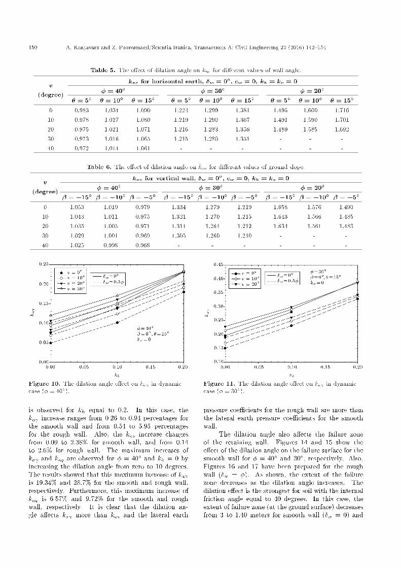
150 A. Keshavarz and Z. Pooresmaeil/Scientia Iranica, Transactions A: Civil Engineering 23 (2016) 142{154
Table 5. The e�ect of dilation angle on kac for di�erent values of wall angle.
v kac for horizontal earth, �w = 0�, cw = 0, kh = kv = 0
(degree) � = 40� � = 30� � = 20�
� = 5� � = 10� � = 15� � = 5� � = 10� � = 15� � = 5� � = 10� � = 15�
0 0.983 1.034 1.090 1.224 1.299 1.381 1.495 1.600 1.71610 0.978 1.027 1.080 1.219 1.290 1.367 1.491 1.590 1.70120 0.975 1.021 1.071 1.216 1.283 1.358 1.489 1.585 1.69230 0.973 1.016 1.065 1.215 1.280 1.351 - - -40 0.972 1.014 1.061 - - - - - -
Table 6. The e�ect of dilation angle on kac for di�erent values of ground slope.
v kac for vertical wall, �w = 0�, cw = 0, kh = kv = 0
(degree) � = 40� � = 30� � = 20�
� = �15� � = �10� � = �5� � = �15� � = �10� � = �5� � = �15� � = �10� � = �5�
0 1.053 1.019 0.979 1.334 1.279 1.219 1.658 1.576 1.49010 1.043 1.011 0.975 1.321 1.270 1.215 1.643 1.566 1.48520 1.035 1.005 0.971 1.311 1.264 1.212 1.634 1.561 1.48330 1.029 1.001 0.969 1.305 1.260 1.210 - - -40 1.025 0.998 0.968 - - - - - -
Figure 10. The dilation angle e�ect on ka in dynamiccase (� = 40�).
is observed for kh equal to 0.2. In this case, theka increase ranges from 0.26 to 0.94 percentages forthe smooth wall and from 0.54 to 5.95 percentagesfor the rough wall. Also, the kaq increase changesfrom 0.09 to 2.38% for smooth wall, and from 0.14to 2.6% for rough wall. The maximum increases ofka and kaq are observed for � = 40� and kh = 0 byincreasing the dilation angle from zero to 10 degrees.The results showed that this maximum increase of ka is 19.34% and 28.7% for the smooth and rough wall,respectively. Furthermore, this maximum increase ofkaq is 6.57% and 9.72% for the smooth and roughwall, respectively. It is clear that the dilation an-gle a�ects ka more than kaq and the lateral earth
Figure 11. The dilation angle e�ect on ka in dynamiccase (� = 30�).
pressure coe�cients for the rough wall are more thanthe lateral earth pressure coe�cients for the smoothwall.
The dilation angle also a�ects the failure zoneof the retaining wall. Figures 14 and 15 show thee�ect of the dilation angle on the failure surface for thesmooth wall for � = 40� and 30�, respectively. Also,Figures 16 and 17 have been prepared for the roughwall (�w = �). As shown, the extent of the failurezone decreases as the dilation angle increases. Thedilation e�ect is the strongest for soil with the internalfriction angle equal to 40 degrees. In this case, theextent of failure zone (at the ground surface) decreasesfrom 3 to 1.40 meters for smooth wall (�w = 0) and

A. Keshavarz and Z. Pooresmaeil/Scientia Iranica, Transactions A: Civil Engineering 23 (2016) 142{154 151
Figure 12. The dilation angle e�ect on kaq in dynamiccase (� = 40�).
Figure 13. The dilation angle e�ect on kaq in dynamiccase (� = 30�).
Figure 14. The dilation angle e�ect on the failure zone(� = 40�, �w = 0).
from 3.48 to 1.59 meters for rough wall (�w = �).Considering the dilation e�ect on the failure zoneshows that the dilation angle a�ects the failure zoneconsiderably and is more e�ective for rough retainingwalls. The Monobe-Okabe (M-O) failure surfaces [24]
Figure 15. The dilation angle e�ect on the failure zone(� = 30�, �w = 0).
Figure 16. The dilation angle e�ect on the failure zone(� = 40�, �w = �).
Figure 17. The dilation angle e�ect on the failure zone(� = 30�, �w = �).
are also shown in the Figures 14-17. As shown, forsmooth walls, the M-O and associated ZEL failuresurfaces are the same; but for rough walls, the failuresurfaces are not linear and the M-O and associated ZELfailure surfaces are somewhat di�erent.

152 A. Keshavarz and Z. Pooresmaeil/Scientia Iranica, Transactions A: Civil Engineering 23 (2016) 142{154
4. Conclusions
In order to evaluate the lateral earth pressure on theretaining walls, the static and seismic lateral earthpressure coe�cients have been calculated using themethod of zero extension lines. The results of thelateral earth pressure coe�cients due to the soil unitweight, surcharge, and soil cohesion are presented forassociated and non-associated ow rules. The lateralearth pressure coe�cients were found to be compatiblewith other methods. A low di�erence between ZELmethod and other methods is observed and the di�er-ence is equal to zero in many cases. The in uence ofthe di�erent parameters on the lateral earth pressurecoe�cients has been explored.
For associative soils, ka and kaq decrease byincreasing each of the soil friction angle, wall angle,and ground slope parameters, and ka decreases byincreasing the soil-wall interface friction angle. Also,increasing the soil friction angle and ground slope anddecreasing the wall angle decrease kac. The seismiclateral earth pressure coe�cient ka for associative soilsincreases as the horizontal and vertical pseudo-staticcoe�cients increase.
For non-associative soils, the dilation angle a�ectsthe lateral earth pressure coe�cients, slightly. Byincreasing the dilation angle, ka increases for plusvalues of the wall angle and ground slope, and decreasesfor minus values of the wall angle and ground slope;kac decreases and kaq increases. The dilation anglee�ect on the failure zone of the retaining wall is suchthat the extent of the failure zone in active casedecreases considerably as the dilation angle increases.The dilation angle e�ects on ka , kaq, and the failurezone of the retaining wall for the rough wall are morethan those for the smooth wall.
Nomenclature
q Surcharge� Ground slope� Wall angleH Height of the retaining wallc Cohesion of the soil� Friction angle of the soil Unit weight of the soilv Dilation angle of the soil�w Friction angle of the soil-wall interfacecw Adhesion of the soil-wall interface�0 Normal stress on the ground surface�0 Shear stress on the ground surface�f Normal stress on the wall�f Shear stress on the wall
p Average stress Angle between �1 and the horizontal
axisp0 Average stress on the ground surface 0 The angle on the ground surfacepf Average stress on the wall f The angle on the wallfx; fz Body forces along x and z directionskh; kv Horizontal and vertical pseudo-static
earthquake coe�cients
d"+; d"� Lengths of plus and minus zeroextension lines
ka Lateral earth pressure coe�cient dueto the unit weight of the soil
kaq Lateral earth pressure coe�cient dueto the surcharge
kac Lateral earth pressure coe�cient dueto the cohesion of the soil
References
1. Peng, M. and Chen, J. \Slip-line solution to ac-tive earth pressure on retaining walls", G�eotechnique,63(12), pp. 1008-1019 (2013).
2. Sokolovskii, V., Statics of Soil Media, Scienc. Publ.,Butterworth, London (1960).
3. Askari, F., Totonchi, A. and Farzaneh, O. \Applicationof admissible stress �elds for computation of passiveseismic force in retaining walls", Sci. Iran, 19(4), pp.967-973 (2012).
4. Chen, W. and Liu, X. \Limit analysis in soil me-chanics", Developments in Geotechnical Engineering(1990).
5. Iskander, M., Chen, Z., Omidvar, M., Guzman, I. andElsherif, O. \Active static and seismic earth pressurefor c�� soils", Soils Found., 53(5), pp. 639-652 (2013).
6. Lin, Y.L., Leng, W.M., Yang, G.L., Zhao, L.H., Li,L. and Yang, J.S. \Seismic active earth pressure ofcohesive-frictional soil on retaining wall based on a sliceanalysis method", Soil Dyn. Earthquake Eng., 70, pp.133-147 (2015).
7. Roscoe, K.H. \The in uence of strains in soil mechan-ics", Geotechnique, 20(2), pp. 129-170 (1970).
8. James, R. and Bransby, P. \A velocity �eld for somepassive earth pressure problems", Geotechnique, 21(1),pp. 61-83 (1971).
9. Habibagahi, K. and Ghahramani, A. \Zero extensionline theory of earth pressure", J. Geotech. Eng. Div.,105(7), pp. 881-896 (1979).
10. Anvar, S. and Ghahramani, A. \Equilibrium equationson zero extension lines and its application to soil

A. Keshavarz and Z. Pooresmaeil/Scientia Iranica, Transactions A: Civil Engineering 23 (2016) 142{154 153
engineering", Iran J. Sci. Technol., 21(1), pp. 11-34(1997).
11. Jahanandish, M. \Development of a zero extensionline method for axially symmetric problems in soilmechanics", Sci. Iran, 10(2), pp. 203-210, Elsevier(2003).
12. Jahanandish, M. and Keshavarz, A. \Evaluation ofstatic and dynamic stability of slopes by the zeroextension line method", in Fourth International Con-ference of Earthquake Engineering and Seismology,SEE4, Tehran, Iran (2003).
13. Jahanandish, M., Mansourzadeh, S. and Emad, K.\Zero extension line method for three-dimensionalstability analysis in soil engineering", Iran J. Sci.Technol. B, 34(B1), pp. 63-80 (2010).
14. Jahanandish, M., Veiskarami, M. and Ghahramani, A.\Investigation of foundations behavior by implementa-tion of a developed constitutive soil model in the ZELmethod", Int. J. Civ. Eng., 9(4), pp. 293-306 (2011).
15. Behpoor, L. and Ghahramani, A. \Zero extension linetheory of static and dynamic bearing capacity", inFrac, H�uft Asian Regional Conference on Soil Mechan-ics and Foundation Engineering (1987).
16. Behpoor, L. and Ghahramani, A. \Recommendationfor evaluation of dynamic earth pressure on retainingstructures for Iranian earthquake code", in SecondInternational Seminar on Soil Mechanics and Foun-dation Engineering of Iran, Shiraz University, Iran(1993).
17. Behpoor, L. and Ghahramani, A. \Undrained bearingcapacity of clay by zero extension line", in Proceedingsof the International Conference on Soil Mechanics andFoundation Engineering - International Society for SoilMechanics and Foundation Engineering, A.A. Balkema(1994).
18. Veiskarami, M., Jahanandish, M. and Ghahramani, A.\Prediction of foundations behaviors by a stress levelbased hyperbolic soil model and the ZEL method",Computational Methods in Civil Engineering, 1(1), pp.37-54 (2010).
19. Veiskarami, M., Jahanandish, M. and Ghahramani,A. \Application of the ZEL method in the predictionof foundation bearing capacity considering the stresslevel e�ect", Soil Mech. Found. Eng., 47(3), pp. 75-85(2010).
20. Veiskarami, M., Jahanandish, M. and Ghahramani,A. \Prediction of the bearing capacity and load-displacement behavior of shallow foundations by thestress-level-based ZEL method", Sci. Iran, 18(1), pp.16-27 (2011).
21. Benmeddour, D., Mellas, M., Frank, R. and Mabrouki,A. \Numerical study of passive and active earthpressures of sands", Comput. Geotech., 40, pp. 34-44(2012).
22. Lee, I. and Herington, J. \A theoretical study of the
pressures acting on a rigid wall by a sloping earth orrock �ll", Geotechnique, 22(1), pp. 1-26 (1972).
23. Shiau, J. and Smith, C. \Numerical analysis of passiveearth pressures with interfaces", in Proceedings of theIII European Conference on Computational Mechanics(ECCM 2006), Springer-Verlag (2006).
24. Kramer, S.L., Geotechnical Earthquake Engineering,Prentice Hall, New Jersey (1996).
Appendix
The parameters in Eqs. (14)-(17) are:
tgmp =tan( C + �C) + tan( B + �B)
2; (A.1)
tgmm =tan( C � �C) + tan( A � �A)
2; (A.2)
A3 = pB � pA +A1 + BBmp �Bmm A �A2;(A.3)
A4 = Bmp �Bmm; (A.4)
where:
Bmp =�
��+ ��BCAC
�[(pC + pB) tan�+ 2c] ; (A.5)
A1 = Cmp +Dmp; (A.6)
Cmp = fx �� [(xC � xB)��� (zC � zB) tan�] ; (A.7)
Dmp = fz �� [(xC � xB) tan�+ (zC � zB)��] ; (A.8)
Bmm = ��
��+ ��ACBC
�[(pC + pA) tan�+ 2c] ;
(A.9)
A2 = Cmm +Dmm; (A.10)
Cmm = fx �� [(xC � xA)��� (zC � zA) tan�] ; (A.11)
Dmm = fz �� [�(xC � xA) tan�+ (zC � zA)��] :(A.12)
Biographies
Amin Keshavarz is currently an Assistant Professorof Civil Engineering in the School of Engineeringat Persian Gulf University, Iran. He received hisBSc degree in Civil Engineering from Persian GulfUniversity in 1997. He also received his MSc andPhD degrees in Civil Engineering (Soil Mechanics andFoundations) from Shiraz University, Iran, in 2000and 2007, respectively. His research interests arestress characteristics and ZEL methods, soil dynamicsand geotechnical earthquake engineering, and stability

154 A. Keshavarz and Z. Pooresmaeil/Scientia Iranica, Transactions A: Civil Engineering 23 (2016) 142{154
analysis of reinforced and unreinforced soil slopes andretaining walls.
Zahra Pooresmaeil received her BSc degree in CivilEngineering from Persian Gulf University, Iran, in2011. She was accepted for MSc degree in 2012. Her
�eld of study was Soil Mechanics and Foundations.In 2014, she attended the 2nd Iranian Conferenceon Geotechnical Engineering and the 8th NationalCongress on Civil Engineering and presented someparts of her thesis. She received her MSc degree fromPersian Gulf University in 2014.