Embed Size (px)
Citation preview


Evaluation of the SPEDE instrument
on SMART-1
Mikael Backrud
May 2007
Royal Institute of Technology (KTH) Report - TRITA-EE 2007:023

Abstract The Spacecraft potential, electron and dust experiment (SPEDE) was one of the instruments
on-board SMART-1, Europe’s first lunar mission. One operational mode of the instrument
was to measure variations in the low-frequency wave intensity around the Moon and in the
Earth’s magnetosphere. The algorithm on-board SPEDE has been simulated and compared
with reliable algorithms to see how the resource saving measures have affected the data. The
data variability was investigated statistically relative the spacecraft location and solar wind
conditions. The analysis showed that the flight algorithm gives an approximate power
spectrum, underestimating the signal power and gives a small distortion. Statistics showed that
the data did not contain any variance of significant levels relative the bins. The possible source
of error is the limited dynamic range of the wave mode measurement.


Acknowledgements I wish to thank the following people, who have in some way contributed to the success of my
work.
Lars Blomberg The Royal Institute of Technology (KTH), Stockholm, Sweden
Annsi Mälkki The Finnish Meteorological Institute (FMI), Helsinki, Finland
Walter Schmidt The Finnish Meteorological Institute (FMI), Helsinki, Finland
Per-Arne Lindqvist The Royal Institute of Technology (KTH), Stockholm, Sweden


Contents
Abbreviations.....................................................................................................................1 Chapter 1: Introduction .................................................................................................... 3 1.1 Background ........................................................................................................................ 3 1.2 Thesis definition................................................................................................................. 4
1.2.1 Goals..................................................................................................................................................4 1.2.2 Methodology ....................................................................................................................................4 1.2.3 Specific tasks ....................................................................................................................................4
Chapter 2: Theory............................................................................................................. 5 2.1 The Solar wind.................................................................................................................... 5
2.1.1 Interaction with magnetized planets.............................................................................................6 2.1.2 Interaction with unmagnetized bodies.........................................................................................6
2.2 The SPEDE instrument ..................................................................................................... 8 2.2.1 Hardware description......................................................................................................................8 2.2.2 Plasma wave measurement ............................................................................................................9
2.3 The Wavelet transform......................................................................................................10 2.3.1 The Continuous wavelet transform............................................................................................10 2.3.2 The Discrete wavelet transform..................................................................................................14 2.3.3 Daubechies D4 wavelet transform .............................................................................................16 2.3.4 The Flight algorithm .....................................................................................................................18
Chapter 3: Methodology..................................................................................................21 3.1 The SPEDE simulation ....................................................................................................21
3.1.2 Analytical approach.......................................................................................................................27 3.1.3 Cluster data examples ...................................................................................................................27
3.2 Data binning......................................................................................................................28 3.2.1 Earth’s magnetosphere .................................................................................................................28 3.2.2 Lunar eclipse ..................................................................................................................................28 3.2.3 Altitude............................................................................................................................................29 3.2.4 Local time & Latitude ...................................................................................................................29 3.2.5 Solar wind conditions ...................................................................................................................30
3.3 Data statistics ....................................................................................................................31 3.3.1 Average power spectrum..............................................................................................................31 3.3.2 Normalized average power spectrum.........................................................................................32
Chapter 4: Results ...........................................................................................................33 4.1 The SPEDE simulation ....................................................................................................33 4.2 Data statistics ....................................................................................................................42
4.2.1 Spacecraft position ........................................................................................................................42 4.2.2 Solar wind parameters...................................................................................................................42

Chapter 5: Discussion .....................................................................................................47 5.1 The Absolute spectrum.....................................................................................................47 5.2 The Statistics .....................................................................................................................48 5.3 Future studies....................................................................................................................48 Chapter 6: Conclusions ...................................................................................................49 Appendix A: MATLAB programs ...................................................................................51 A.1 Flight algorithm simulation routines................................................................................51 A.2 Visualization routines .......................................................................................................52 A.3 Binning routines................................................................................................................57 A.4 Analysis routines ...............................................................................................................58 A.5 General routines ................................................................................................................60 References .......................................................................................................................61

1
Abbreviations AS (Absolute Spectrum)
ACE (Advanced Composition Explorer)
ESA (European Space Agency)
FMI (Finnish Meteorological Institute)
VFC (Voltage to Frequency Converter)
GSE (Geocentric Solar Ecliptic)
LSE (Lunacentric Solar Ecliptic)
PSD (Power Spectral Density)
SMART-1 (Small Missions for Advanced Research in Technology One)
SPEDE (Spacecraft Potential, Electron and Dust Experiment)
SS (Squared Spectrum)
SW (Solar Wind)
SZA (Solar Zenith Angle)

2

3
Chapter 1
Introduction
1.1 Background The 27th of September 2003, SMART-1 was launched into space by an Ariane-5 from Kourou
as the first European Lunar expedition. The Spacecraft Potential, Electron and Dust
experiment (SPEDE) was one of the instruments on-board the SMART-1 spacecraft. The
instrument consisted of the electronics inside the spacecraft connected with two Langmuir
probes on 60 cm carbon fibre booms at opposite sides of the spacecraft.
The instrument was to monitor disturbances induced by the ion propulsion system and the
variability of low-frequency wave intensities in the space plasma around the Moon, which is
sometimes located inside the Earth’s magnetosphere. [1]
In this report the wave mode has been evaluated regarding the impact of the technical
limitations on the experimental results. The evaluation comprises an analysis of the data
treatment and statistical studies of data variability for different spacecraft positions and solar
wind conditions.
The analysis was through simulation in MATLAB by development of a SPEDE simulator and
binning of measurement data. The binning was defined according to the satellite position and
solar wind parameters from the ACE satellite.

4
1.2 Thesis definition
1.2.1 Goals
To evaluate the SPEDE instrument as regards wave measurements in the range 10 Hz to 5
kHz and to do a preliminary analysis of the wave data collected in lunar orbit.
1.2.2 Methodology
To analyze the way the wave data are processed on-board including understanding the wavelet
transform and output in physical terms. To statistically analyze the SPEDE wave data by
binning according to SMART-1 spacecraft position relative the Moon, the Earth’s
magnetosphere and solar wind conditions.
1.2.3 Specific tasks
To understand the Daubechies wavelet transform used on-board by analysis, theoretically and
numerically, by comparing the “absolute value” spectrum to the conventional power spectrum.
To develop MATLAB routines for spacecraft position, visualization and analysis. Thereby
analyze the data set for possibility of correlation with numerical modeling.

5
Chapter 2
Theory The chapter includes a brief introduction about the Solar wind, a description of the SPEDE instrument and an
overview of the Wavelet transform and its application on SPEDE.
2.1 The Solar wind As the extreme heat arises towards the Sun’s outer part called the corona, it reaches a
boundary with a large pressure difference against the interstellar medium. This forces ionized
gas out from the sun into space consisting of protons, electrons and a small part of ionized
helium. This storm of particles is called the Solar wind and has been an important subject for
studies regarding its interactions with planets, comets, dust particles and cosmic rays. [3]
Forcing through space the plasma contains magnetic field lines that originate at the Sun
directed outwards in the elliptical plane. The magnetic field is “frozen in”, meaning that the
field lines follow the expansion and movement of the space plasma. This puts the field lines in
a direction of 45 degrees at Earth orbit relative to the Sun-Earth line.
As the solar wind sweeps around the Earth’s magnetic field, at speeds from about 200 km sec-1
up to 1000 km sec-1, it causes both trouble and temporary enchantment such as magnetic
storms and auroras. [3]

6
2.1.1 Interaction with magnetized planets
The magnetic field’s interaction with the solar wind is governed by a balance between the solar
wind thermal and dynamic pressure and the Earth’s magnetic field lines.
This contracts the magnetosphere on the dayside and extends it on the night side. The harder
the wind blows, the more it pushes the magnetic field lines away, until equilibrium is reached.
[3]
The boundary is called the Magnetopause with an average distance on the dayside of around 10
RE and an extended part on the night side called the Magnetotail. The Magnetotail is often
approximated as a cylinder with radius about 20 - 30 Earth radii that stretch out behind the
Earth in the opposite direction to the Sun. [3]
2.1.2 Interaction with unmagnetized bodies
When a body or planet in the solar wind has no self supporting magnetic field, the solar wind
might induce a magnetic field, if the core is conductive. This prevents the outer magnetic fields
to penetrate the planet. But since the magnetic field is close to the body surface, there is no
shielding against incoming particles. [3]
The solar wind is not affected on the dayside of the planet. But on the night side a wake is
created, consisting of more tenuous plasma. This affects the magnetic streamlines since the
magnetic field is frozen in, as mentioned earlier. The effect is somewhat like the streamlines
from a supersonic bullet with variance in density and curls. [3]
A thin layer of particles surrounds the planet that sometimes gets ionized and starts to gyrate
around the magnetic field lines. They travel in the direction of the Solar wind and oscillate in a
plane with normal parallel to the magnetic field lines. These ions are often thrown back into
the planet unless they are positioned propitious and have a large gyro radius. Then they might
fly past the planet and get picked up by the solar wind, thereby called pickup ions. The gyro
radius is given by
(2.1) /gr mu eB⊥=
7
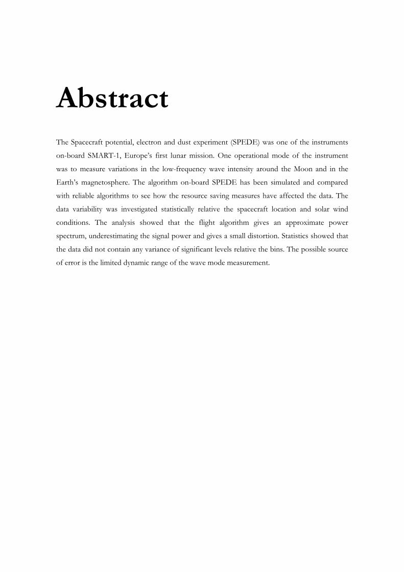
where m is the ion mass, u┴ is the solar wind speed perpendicular to the magnetic field lines, e
is the electron charge and B the magnetic field strength as illustrated in figure (2.2). [3]
Figure 2.2: Illustrating a pickup ion on the front side of the
Moon where u is the solar wind speed, B is the magnetic field
and E is the electric field generated as the cross product of the
other two.

8
2.2 The SPEDE instrument The Spacecraft Potential, Electron and Dust Experiment (SPEDE) was designed by the FMI
(Helsinki, Finland), ESA/SSD (Noordwijk, The Netherlands), IRFU (Uppsala, Sweden) and
KTH (Stockholm, Sweden). [8]
The two main objectives were:
• To monitor disturbances induced by the ion propulsion system by measurements of
electron flux, wave electric fields and variability of spacecraft potential. [2]
• To measure the variability in electron density and wave electric fields during Earth
spiraling phase and moon phase. [2]
This evaluation has been regarding the wave mode for the second objective. That was to
measure the variability in wave electric fields around the moon.
2.2.1 Hardware description
The instrument had two cylindrical Langmuir probes mounted on the tips of two 60 cm
carbon fibre booms on either side of the spacecraft. The booms had a tip diameter of 22 mm
and bottom diameter of 40 mm and were connected to the internal electronics with a triaxial
cable. The sensor tip was of Titanium Nitrade foil and had a width of 100 mm, giving total
sensor areas of 73.8 cm2. One boom failed during deployment leaving only one sensor for
measurements. [1]
The triaxial cable was connected to the combined pre-amplifier bias driver with a variable bias
voltage of +/-13 V used as fixed or set to ground value. The result is two modes, one
measuring current and the other measuring voltage, that is the Langmuir mode and the Electric
field mode. [1]
The signal then passed a voltage-to-frequency-converter (VFC) transforming the current-
driven voltage drop between +12 and –14 V into frequencies between 0.1 and 190 kHz. For
plasma wave measurements with 10 kHz sample frequency, this gives a dynamic range of 20

9
levels between 0 and 19. Where +5 V gives 0 and –14 V gives 19. That was treated by a
Daubechies D4 Wavelet transform in the 16-bit RISC processor. [1]
The low resolution of the signal with only one quantization level for each volt is motivated
against the second alternative for its linearity and computational feasibility. Since the other
alternatives numbers would be too large for the 16-bit processor to handle and it would give
1/x dependence between the frequency and voltage. That was not as good as the low-
resolution solution.
2.2.2 Plasma wave measurement
The plasma wave measurement used a constant bias voltage and sampling frequency of 10 kHz
for exactly 0.2048 seconds, giving a sample length of 2048. After the VFC the quantized signal
was treated with a fast wavelet transform dividing the signals frequency information into 10
predefined frequency bins. The highest bin was given maximum frequency of 5 kHz and
minimum of 2.5 kHz that was the highest frequency for the next bin, and so on in descending
order. This gives the bins half of each bandwidth with the lowest bin consisting of frequencies
about 10 Hz. [1]
The signal energy is conserved through the transformation, which makes it possible to get the
signal energy for each frequency bin by summing the squares of the transformation. Since the
processor could not handle such computations, the bin coefficients absolute values were
summed giving an absolute spectrum instead of the squared spectrum. That has been evaluated
in this report, described in more detail in chapter (2.3).

10
2.3 The Wavelet transform
2.3.1 The Continuous wavelet transform
The Continuous wavelet transform (CWT) is an alternate solution to Short Time Fourier
Transform (STFT). The Wavelet transform is a multi resolution approach which is
accomplished by changing the windowing function through the transform. This implies that
the high-frequency components get small frequency resolution and high time resolution and
the low-frequency components get small time resolution and high frequency resolution, as
illustrated in figure (2.3). That can be especially useful on applications when there are short
periods of high-frequent signals and longer times of low-frequent signals. The window
functions used are the Mexican hat function or the Morlet function. [5]
Figure 2.3: Illustrating the time and frequency resolution
dependence.

11
The Mexican hat function is the second derivative of a normalized Gaussian function
(2.2) 222
2
23
1( ) 12
t tt e σ
σπσ
− ⎛ ⎞= −⎜ ⎟
⎝ ⎠ψ
where represents the chosen width of the window. The Morlet wavelet is defined as
(2.3) 2
22( )t
iatw t e e σ−
=
where a is a modulation parameter and the window width. [5]
Figure 2.4: The Mexican hat function with equal to 1.

12
Figure 2.5: Illustration the Morlet function with equal to 1
and a equal to 5.3 [7].
The continuous transform is defined as
(2.4) 1( , ) ( , ) ( )x xtCWT s s x t dtssττ τ ∗ −⎛ ⎞= Ψ = ⎜ ⎟
⎝ ⎠∫ψ ψ ψ
where is the translation and s is the scale which represents the window position and width.
The transformation starts with a narrow window at the beginning of the signal represented by
a small value for s and equal to 0. Then the signal is multiplied with the window ψ , also
called the Mother wavelet, and integrated over all times. Then the result is divided by the
square root of s for energy conservation. After the integration, is increased by a small
number i.e. the window is moved slightly forward in time and then integrated over all times.
When the entire time interval has been treated the scale is increased and translation is set to
zero again. This is repeated until the desired scales are calculated and as the scales get higher,
the window gets broader leading to a smoothed time distinction. That is the reason for the
resolution phenomenon described earlier in this chapter. [5]

13
Figure 2.6: Example sound file of sampling frequency 44100 Hz
consisting of 4792 sample elements.
Figure 2.7: The Spectrogram of the example sound file i.e. the
CWT squared showing that the first part of the sound is louder and
the later part is slightly higher in frequency.

14
2.3.2 The Discrete wavelet transform
The Discrete wavelet transform is the sampled version of the continuous case where the
window is replaced with high-pass and low-pass filters. Because of down sampling the discrete
transform is fast and only requires small computational resources.
The first step in the Discrete wavelet transform (DWT) for a signal with sampling frequency fs
and length N is to filter half of the upper bandwidth with a simultaneous down sampling of a
factor 2 and normalize it according to conservation of energy. Then the lower half of the
bandwidth is filtered with a low-pass filter with simultaneous down-sampling of a factor 2,
normalized as with the previous filtering. This will give a number of N/2 level 1 wavelet
coefficients containing frequency information from fs/4 to fs/2 according to the Nyquist
theorem. Then the low pass filtered and down sampled coefficients are treated the same way as
the original signal, resulting in a high pass and a low pass filtered part. This procedure is
performed iteratively until the entire signal has been transformed, as illustrated in figure (2.8).
The resolution varies similar to the continuous case, as illustrated in figure (2.3). [5]

15
Figure 2.8: The DWT for a signal of N samples and sampling frequency fs.
f = 0 ~ fs/2 n = N
f = fs/4 ~ fs/2 n = N/2
high
low
f = 0 ~ fs/4 n = N/2
f = fs/8 ~ fs/4 n = N/4
high
low
f = 0 ~ fs/8 n = N/4
f = fs/16 ~ fs/8 n = N/8
high
low…
Signal, fs, N DWT coefficients
f = 0 ~ fs/N n = 2
f = 0 ~ fs/N n = 1
high
…
Level 1
Level 2
Level 3
Level log2(N)
16
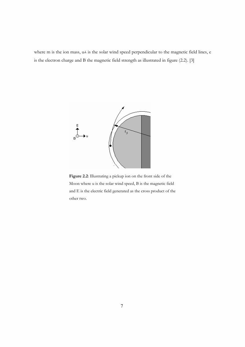
2.3.3 Daubechies D4 wavelet transform
There are many versions of the discrete wavelet transform resulting in different accuracy
depending of the complexity of the filtering. The version used by SPEDE is the Daubechies
D4 Wavelet transform that is one of the best transforms since it makes it possible to recreate
the original signal perfectly. It uses four coefficients for filtering defined by
(2.5) 1 3 3 3 3 3 1 34 2 4 2 4 2 4 2
h⎡ ⎤+ + − −= ⎢ ⎥⎣ ⎦
(2.6) [ ](3) (2) (1) (0)g h h h h= − −
that is used in the four-point filtering as
(2.7) 3
0( ) (2 )j
jc i g s i j
=
= ⋅ +∑
(2.8) 3
0( ) (2 )j
ja i h s i j
=
= ⋅ +∑
where s is the signal, g is the high-pass filter or wavelet function, c is the wavelet coefficients,
h is the low-pass filter or scaling function and a is the low-passed signal. [6]
Figure 2.9: The Daubechies D4 Wavelet function. [10]

17
Since the wavelet function and scaling function are normalized according to energy
conservation meaning that the sum of the squared signal is equal to the sum of the squared
wavelet coefficients. It is possible to get the power for a specific frequency bin by squaring the
coefficients and integrate over time. This gives an estimate of the frequency content of the
signal and the signal power.
(2.9) log22 1
2,
0( )
N l
l kk
spectrum l c− −
=
= ∑
Figure 2.10: The power spectrum from the DWT of the sound file used in the
CWT examples.

18
Figure 2.11: The frequency content of the FFT for the same sound file revealing
the true frequency peak around 400 Hz.
2.3.4 The Flight algorithm
Technical limitations in the hardware made it impossible to perform the squaring of the
wavelet coefficients when calculating the power spectrum. The solution was to sum the
absolute values of the coefficients instead.
Since the square of the summed elements contained the desired power from theory, plus the
double cross product of the vector, it was possible to derive an approximated power spectrum
with the sum of the transformed elements given by
(2.10) 1
n
kk
S c=
=∑
where S is the sum and ck are the coefficients that give the following when squared.
(2.11) 2
2 2 2 2 21 2 1 2 2 3 1
1 1... 2 2 ... 2
n n
k n n kk k
S c c c c c c c c c c c extra= =
⎛ ⎞= = + + + + + + + = +⎜ ⎟⎝ ⎠∑ ∑
To approximate the extra coefficients, the double cross product, it was necessary to use the
average element to replace the unknown elements. By squaring and adding the average

19
elements together and subtracting this from the squared sum. An approximation of the power
was obtained where the average element was given by
(2.12) 1c SN
⟨ ⟩ =
and the extra double cross product calculated according to
(2.13) ( )
22 2
2
! 1 ( 1) 12 2 12! 2 !k l kl
k l
N N Nextra c c S S SN N N N
δ −⎛ ⎞ ⎛ ⎞= ⋅ ≈ ⋅ = ⋅ = −⎜ ⎟ ⎜ ⎟− ⎝ ⎠ ⎝ ⎠∑∑
Then the approximated power was obtained by elimination of the error from the squared sum.
(2.14) 2
2 2 11 1 SP S extra SN N
⎛ ⎞⎛ ⎞= − = − − =⎜ ⎟⎜ ⎟⎝ ⎠⎝ ⎠
This derived approximation was used to calculate the power spectrum from the SPEDE data.
The problem is to estimate how large error the cross product withholds resulting in a total
error relative the squared spectrum and what effect it might have on the results.
Analytically the error can be derived by dividing the coefficients as the average coefficient plus
the coefficient deviation from the average as
(2.15) i ic a d= +
where ci is the coefficient, a is the average in formula (2.12) and di is the coefficient deviation
from the average coefficient. This makes the conventional spectrum calculated as
(2.16) ( )22 2 2 2 22i i i i iP c a d Na a d d Na d= = + = + ⋅ + = +∑ ∑ ∑ ∑ ∑
where N is the number of coefficients which calculates the absolute spectrum as
(2.17)
( ) ( ) ( ) ( )2 2 2 22 21 1 1 2i i i i iP c a d a d Na a d d NaN N N
= = + = + = + + =∑ ∑ ∑ ∑ ∑ ∑ ∑
This means that the difference in power is given by the sum of the squared coefficient
deviation.

20
(2.18) 2 2 2 2i iP P Na d Na d− = + − =∑ ∑

21
Chapter 3
Methodology This chapter describes of the methods used for analysis of the data processing and the statistics. That is the
SPEDE simulation, the data binning and the central numbers used for statistical analysis.
3.1 The SPEDE simulation
By sampling the potential difference between the satellite body and the Langmuir probe at 10
kHz, a series of gathered data were analyzed regarding its frequency information.
The wave mode of the instrument was engaged at the end of every measurement sequence,
where a sample of 2048 elements was transformed into a wavelet for further analysis.
The simulation consisted of the signal generator, a VFC for quantization of the signal, a
Daubechies D4 wavelet transformation, the squared spectrum calculations and the absolute
spectrum calculations. Where the signal was sine shaped about SPEDE’s measurement range
between 5V and -14V. That passed through the VFC which mirrored it down on a discrete
interval between 0 and 19, where each integer step represented one volt. [1]
The quantized signal was transformed according to the Daubechies D4 wavelet transformation
and stored in a matrix of 1024 columns and 10 rows. The first filtration was stored in row one
and the second in the next row and so on as described in chapter (3.3).
The signals of interest are the continuous and discrete signal where the ideal spectrum is the
continuous signal squared spectrum (SS). The real case however is the discrete signal absolute

22
spectrum (AS) that compared with the conventional spectrum visualized the effect of the AS
calculations.
The signal below is a small signal but still visible after the quantization since it oscillates
between the quantization levels at 0 V and 1 V.
Figure 3.1: Signal of 250Hz with amplitude 0.5V and an offset of 0.5V
with random phase between 0 and 57.3 degrees. That was chosen because
of the measurement data seems to have a peak in the same frequency bin.
When the signal passes through the VFC it gets quantized and the result is visible bellow. The
previous oscillations between 0 V and 1 V have become oscillations between the quantization
levels of 4 and 5.

23
The resulting discrete signal seems to represent the continuous signal in a good way and will
probably result in a correct spectrum. The problem is that the continuous signal is sine shaped
and the discrete is square, which means that the discrete has more signal energy. The other
problem is the approximating absolute spectrum (AS), as described in chapter 2.3.4 and 4.1.
Figure 3.2: Quantization of the signal in figure (3.1).
The spectrum calculations from both the continuous and discrete signal is presented below. It
is clearly visible that the SS and AS give different results and there is also the effect of
exaggeration due to the quantization in the SPEDE spectrum. The continuous signal shows
the effect from the absolute spectrum with an underestimated of about 20%.

24
Figure 3.3: The dotted black curve shows the continuous signal SS, the gray curve
shows the continuous signal AS and the black curve shows the discrete signal AS.
The signal was a 250 Hz sine wave with amplitude 0.5V and an offset 0.5V with a
random phase between 0 and 57.3 degrees. See figure (3.1) and (3.2).
The next step was to introduce noise that was chosen to simulate the SPEDE spectra as good
as possible. The noise was white with power of 1 dBW according to the MATLAB white noise
function. The resulting signal after the noise looks messy but since the transformation only
process four points at the time it will not be a problem.

25
Figure 3.4: Signal of 250Hz with amplitude 0.5V and an offset of 0.5V
with white noise at 1dBW.
Figure 3.5: Quantization of the signal in figure (3.7).

26
The power spectrum below shows that by introducing noise to the signal the quantization gets
less important since it uses more of the dynamic range and that the error lies within the AS
calculations.
If the noise would be smaller, the quantization might exaggerate it leading to even higher
powers than in the spectrum in figure (3.3).
The general underestimation due to the AS calculations below is about 30%. This is near the
probable power loss for the SPEDE measurement based on that the measurement spectra
look very similar to this. But compared to Cluster data implementation the underestimation
could be as low as 40%, as described at the end of chapter (4.1).
Figure 3.6: The dotted black curve shows the continuous signal SS, the
gray curve shows the continuous signal AS and the black curve shows the
discrete signal AS. The signal was 250Hz with amplitude 0.5V and offset
0.5V with white noise at 1dBW. See figure (3.7) and (3.8).

27
3.1.2 Analytical approach
To better estimate the power loss from the absolute spectrum, the power calculations were
looped through the entire frequency range for a sine wave. In each loop the ratio between the
traditional and the approximated power was calculated for spectrum peaks higher than 5% of
the highest peak in the desired spectrum. This ensured that only significant error is
encountered. The plots show how the power was affected by random phase, frequency
composition and signal amplitude.
The result was that the absolute spectrum represents a good spectrum shape for most signals.
But there is an underestimation in power for single frequency waves of about 20% from the
conventional spectrum, for white noise about 30% and even down to 50% when inserting a
signal with many close frequency peaks. The most similar signal to the SPEDE measurements
was white noise with a small frequency peak in the 250 Hz frequency bin.
3.1.3 Cluster data examples
To get more realistic signals for a better view of how the approximation affected the data. The
spectrum calculations were made with a short series of Cluster data. The data were sampled
with 9 kHz that is close to the SPEDE sampling frequency of 10 kHz.
When having adapted the Cluster data to the SPEDE measurement range the result was a
power underestimation of about 40%. That is probably the best estimation to compare with
the SPEDE measurement.

28
3.2 Data binning
3.2.1 Earth’s magnetosphere
Since the solar wind gets disturbed by the Magnetopause it is interesting to see how the plasma
wave intensity varies between direct exposure to the Solar wind compared to when protected
by the Earth’s magnetosphere. Therefore the data were binned according to the spacecraft’s
position relative the Earth’s magnetosphere.
From the data the spacecraft position was determined in geocentric solar ecliptic (GSE) and
lunar centric solar ecliptic (LSE) coordinates with the approximation of a cylindrical magneto
tail of radius 25 Earth radii. This made the binning inside the magnetosphere for positions at
negative X within radius of 20 Earth radii in the YZ-plane for GSE coordinates. The next bin
between the solar wind and inside magnetosphere was for negative X within radius of 20 – 30
Earth radii. The complement to these two bins was in the solar wind, the largest bin.
3.2.2 Lunar eclipse
By using the LSE coordinate system, similar to the bins from the magnetosphere, the lunar
eclipse was binned according to the lunar umbra and the lunar penumbra. That is when the
Sun is in partly or total eclipse relative to the spacecraft’s position. The angle for the Moon
shadow is 0.53º, illustrated in figure (3.7).
The interesting part of these bins is to see whether the tenuous wake behind the unmagnetized
body has an effect on the frequency composition or intensity of the plasma waves. It is also
interesting to see if there is any difference between the lunar umbra and penumbra. Possible
expectation is less intensity in the wake than in direct exposure of the Solar wind.

29
Figure 3.7: An exaggerated illustration the lunar
umbra and the lunar penumbra where the theoretical
shadow angle φ is 0.53 degrees.
3.2.3 Altitude
This bin simply divides the lunar surroundings into layers for possibility of closer statistical
investigation from interesting observations.
To get enough data in each bin the altitude bins were defined as in five equidistant intervals.
This resulted in boundaries at 0.5329, 0.8160, 1.0991 and 1.3822 lunar radii above the lunar
surface.
3.2.4 Local time & Latitude
The local time was defined in five areas in the XY-plane in LSE coordinates, as illustrated in
figure (3.8) to the right. The latitude was defined in five areas depending on the spacecrafts
angle to the LSE Z-axis, as illustrated in figure (3.8) to the left. Besides latitude and local time a
similar system was designed with the “polar axis” directed towards the Sun. This made the
latitude equal to the solar zenith angle (SZA) with equal bin definition as the latitude with its
north pole aligned with the LSE Z-axis.

30
Figure 3.8: Latitude and longitude definitions around the Moon where the area
between the dark fields are bin one and five, the areas between the lighter fields
belong to bin 3 and the other to bin 2 and 4.
This bin maps the lunar surface in its symmetrical planes relative the solar wind speed. That
gives possibility together with the altitude bin to accurately specify parts of the lunar
environment giving high resolution statistics.
3.2.5 Solar wind conditions
The next step was to gather data from the ACE spacecraft and correlate it with the SPEDE
data. The parameters chosen for analysis were proton density, proton speed, proton speed
components in GSE, variability of the magnetic field strength (sigma B) and magnetic field
components in GSE and GSM.
The data were then binned as high and low for the proton density to magnetic field strength
and positive and negative for the magnetic field components. The boundaries were defined as
above or below the average of the entire ACE data series. The correlation had a propagation
delay of about one hour.
The solar wind condition could be a major factor impacting the measurement data, with the
most probable outcome as high spectrum power for high values of the solar wind parameters.
The problem was that the correlation is made with an average solar wind speed of 480 km sec-1

31
giving an extra factor of error with unknown quantity in the statistics. Since it is hard to
estimate how static the solar wind is according to one point in space, one hour ago.
3.3 Data statistics
3.3.1 Average power spectrum
By filtering out the bins of special interest it was possible to compare the average power
spectra from the different bins. That would reveal statistical variance in the data with good
overview as the entire data series reached from 20050301 02:44:56 to 20060903 05:41:18 with
total number of 523811 spectra. That was divided into four phases to compare their statistics
and finding characteristic statistical behavior in the data.
Calculating the average power spectrum for different bins and plotting them together gave a
good picture of their differences. The choice of plotting was a surface plot with colormap
reaching from the lowest of dark blue, to yellow up to the highest value of dark red. That
enabled the possibility to plot more than two average spectra in the same plot.
Phase Start End
1 2005-03-01 [02:44:56.650] 2005-08-01 [01:08:00.930]
2 2005-08-01 [03:48:51.220] 2005-12-28 [21:48:54.890]
3 2005-12-29 [00:26:29.019] 2006-05-11 [23:59:35.740]
4 2006-05-12 [00:00:15.740] 2006-09-03 [05:41:18.769]
Table 3.1: The time intervals chosen for the different phases.

32
3.3.2 Normalized average power spectrum
A normalization of spectra was defined for bins with possible statistical variance with too small
variances to notice in the average spectrum. There were two ways of approach resulting in
enhancement of either the dominance in intensity or spectrum shape. These were to normalize
the frequency bins and to normalize the data bins.
When normalizing the frequency bins the highest frequency bin was set to 1 and the lowest to
0. This was made for all frequency bins resulting in a map of squares that show which data bin
that is dominant for different frequency bins. The same normalization was made for the data
bins.
When normalizing the solar wind parameters that contained both positive and negative
numbers, the largest absolute value was set to 1 respectively –1, where 1 was represented in
dark red and -1 was represented in dark blue, leaving 0 at light green.

33
Chapter 4
Results This chapter includes the results from the SPEDE simulation and the data statistics with plots and comments
about their contribution to the experimental results.
4.1 The SPEDE simulation The first case was the absolute optimal signal when the entire dynamic range was used without
disturbing noise. That was a signal with 9.5 V amplitude and offset -4.5 V, see figure (4.1 d).
This gave a power underestimation of about 20% relative the conventional power spectrum
for the continuous signal, the discrete signal and for the spectrum peak. There were
frequencies of perfect power estimation at the borders between the frequency bins due to the
ideal sinusoidal shape of the signal.
(4.1) 4.5 9.5sin(2 )s fπ= − +
The next step was to introduce an uncertainty to the signal frequency resulting in slight
broadening of the spectrum peak. This was made by introducing a random phase to the signal.
The result was an underestimate similar to the optimal case but the peaks in the frequency bin
borders were lost. See figure (4.2 d).
(4.2) 4.5 9.5sin(2 )s fπ ϕ= − + +

34
To approach the real case the signal was reduced 19 times resulting in amplitude 0.5 V and
offset -4.5 V. That showed that the continuous signal still underestimates the power about
20% but the discrete signal gets exaggerated about 50% due to the quantization of the signal.
There was a difference in underestimation as the lower frequencies were exaggerated 30% and
the highest frequencies about 70%. This is since the lower frequency bins only cover part of
the spectrum peak. See figure (4.3 d).
(4.3) 4.5 0.5sin(2 )s fπ ϕ= − + +
The next step was to introduce white noise to the signal which was chosen to be white
Gaussian noise at 1 dBW. This showed to underestimate the conventional power by 30% for
all cases, as seen in figure (4.4).
(4.4) 4.5 0.5sin(2 )s f wgnπ ϕ= − + + +
In the real case the signal does not consist of one single frequency. There might be equally
large signals with frequencies close to each other. Therefore the next case was to introduce 18
more signals with increasing frequencies from the chosen frequency with equally spacing of 10
Hz. This resulted in an overall underestimate of 50% for both cases and an even larger
underestimation for the spectrum peak of 70%. That led once more to a smoothing of the
spectrum shape, as seen in figure (4.5).
(4.5)
4.5 0.5sin(2 ) 0.5sin(2 ( 10) ) ... 0.5sin(2 ( 180) )s f f f wgnπ ϕ π ϕ π ϕ= − + + + + + + + + + +
When inserting the Cluster example into the calculations, the power underestimation reached
about 40% which may be the most probable case to be correlated to the SPEDE
measurements.

35
Figure 4.1: a) Ratio between the continuous signal AS and the continuous signal SS.
b) Ratio between the discrete signal AS and the continuous signal SS.
c) Ratio between the discrete signal AS peak and the continuous signal SS peak.
d) Quantized signal of 80 Hz with amplitude 9.5 V and an offset -4.5 V.
a) b) c) d)

36
Figure 4.2: a) Ratio between the continuous signal AS and the continuous signal SS.
b) Ratio between the discrete signal AS and the continuous signal SS.
c) Ratio between the discrete signal AS peak and the continuous signal SS peak.
d) Quantized signal of 80 Hz with amplitude 9.5 V and an offset -4.5 V and random
phase between 0 and 57.3 degrees.
a) b) c) d)

37
Figure 4.3: a) Ratio between the continuous signal AS and the continuous signal SS.
b) Ratio between the discrete signal AS and the continuous signal SS.
c) Ratio between the discrete signal AS peak and the continuous signal SS peak.
d) Quantized signal of 80 Hz with amplitude 0.5 V and an offset -4.5 V and random
phase between 0 and 57.3 degrees.
a) b) c) d)
-4.5+0.5*sin(f*c+rand);
-4.5+0.5*sin(f*c+rand);
-4.5+0.5*sin(f*c+rand);

38
Figure 4.4: a) Ratio between the continuous signal AS and the continuous signal SS.
b) Ratio between the discrete signal AS and the continuous signal SS.
c) Ratio between the discrete signal AS peak and the continuous signal SS peak.
d) Quantized signal of 80 Hz with amplitude 0.5 V and an offset -4.5 V and random
phase between 0 and 57.3 degrees with white noise at 1 dBW.
a) b) c) d)
-4.5+0.5*sin(f*c+rand)+wgn;
-4.5+0.5*sin(f*c+rand)+wgn;
-4.5+0.5*sin(f*c+rand)+wgn;

39
Figure 4.5: a) Ratio between the continuous signal AS and the continuous signal SS.
b) Ratio between the discrete signal AS and the continuous signal SS.
c) Ratio between the discrete signal AS peak and the continuous signal SS peak.
d) Quantized signal of 21 frequencies separated 10 Hz from the lowest frequency of
80 Hz. All with amplitude 0.5 V and an offset -4.5 V and random phase between 0
and 57.3 degrees with white noise at 1 dBW.
a) b) c) d)
-4.5+0.5*sin([f:10:180]*c+rand)+wgn;
-4.5+0.5*sin([f:10:180]*c+rand)+wgn;
-4.5+0.5*sin([f:10:180]*c+rand)+wgn;

40
Figure 4.6: a) The quantization Cluster data example shifted +0.3 V.
b) The Cluster data example adapted to fit the SPEDE dynamic range.
c) The quantization of the Cluster data example adapted to fit the SPEDE dynamic range.
a) b) c)

41
Figure 4.7: a) The power spectrum for the quantized Cluster data example shifted +0.3 V.
b) The power spectrum for the adapted cluster data example to fit the SPEDE dynamic range.
c) The FFT frequency content for the Cluster data example.
a) b) c)

42
The results from comparing the different spectra are that the SPEDE measurement is
probably underestimated about 40% like the Cluster example. But since the measurements
look more like the white noise simulations with most of its power in the higher frequency bins,
the underestimation might be about 30%.
When assuming that the measurements have good representation in the dynamic range of the
instrument, the underestimation is about 30 to 40%. But if the signal is very small and gets
exaggerated in the quantization, the spectrum power gets very uncertain.
4.2 Data statistics
4.2.1 Spacecraft position
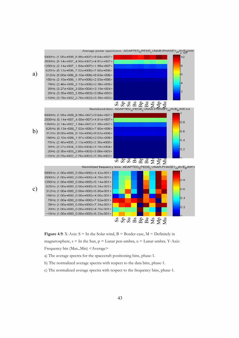
The statistical results from the binned data relative the spacecraft position show that the
average shapes for all the data look very similar throughout the entire time series. There is a
slightly visible increase in amplitude for frequency bins above 250 Hz when the spacecraft is
behind the moon. This conclusion is that either there are no significant variances in
frequencies regarding these bins between 10 Hz and 5 kHz, or that the SPEDE instrument can
not resolve the existing variances.
4.2.2 Solar wind parameters
The statistical results from the binned data relative the solar wind parameters show that the
average shapes for all the data look very similar throughout the entire time series. There is no
consistent variance in power for the average spectrum throughout the different phases. This
implies either that there are no significant variance in frequencies regarding these bins between
10 Hz and 5 kHz, or that the SPEDE instrument can not resolve the existing variances.
43
Figure 4.9: X-Axis: S = In the Solar wind, B = Border case, M = Definitely in
magnetosphere, s = In the Sun, p = Lunar pen-umbra, u = Lunar umbra. Y-Axis:
Frequency bin (Max_Min) <Average>
a) The average spectra for the spacecraft positioning bins, phase-1.
b) The normalized average spectra with respect to the data bins, phase-1.
c) The normalized average spectra with respect to the frequency bins, phase-1.
Ss
Sp
Su
Bs
Bp
Bu
M
s M
p M
u
Ss
Sp
Su
Bs
Bp
Bu
M
s M
p M
u
Ss
Sp
Su
Bs
Bp
Bu
M
s M
p M
u
a) b) c)

44
Figure 4.10: X-Axis: S = In the Solar wind, B = Border case, M = Definitely in
magnetosphere, s = In the Sun, p = Lunar pen-umbra, u = Lunar umbra. Y-Axis:
Frequency bin (Max_Min) <Average>
a) The average spectra for the spacecraft positioning bins, phase-2.
b) The normalized average spectra with respect to the data bins, phase-2.
c) The normalized average spectra with respect to the frequency bins, phase-2.
a) b) c)
Ss
Sp
Su
Bs
Bp
Bu
M
s M
p M
u
Ss
Sp
Su
Bs
Bp
Bu
M
s M
p M
u
Ss
Sp
Su
Bs
Bp
Bu
M
s M
p M
u

45
Figure 4.11: X-Axis: S = In the Solar wind, B = Border case, M = Definitely in
magnetosphere, s = In the Sun, p = Lunar pen-umbra, u = Lunar umbra. Y-Axis:
Frequency bin (Max_Min) <Average>
a) The average spectra for the spacecraft positioning bins, phase-3.
b) The normalized average spectra with respect to the data bins, phase-3.
c) The normalized average spectra with respect to the frequency bins, phase-3.
a) b) c)
Ss
Sp
Su
Bs
Bp
Bu
M
s M
u
Ss
Sp
Su
Bs
Bp
Bu
M
s M
u
Ss
Sp
Su
Bs
Bp
Bu
M
s M
u

46
Figure 4.12: X-Axis: S = In the Solar wind, B = Border case, M = Definitely in
magnetosphere, s = In the Sun, p = Lunar pen-umbra, u = Lunar umbra. Y-Axis:
Frequency bin (Max_Min) <Average>
a) The average spectra for the spacecraft positioning bins, phase-4.
b) The normalized average spectra with respect to the data bins, phase-4.
c) The normalized average spectra with respect to the frequency bins, phase-4.
a) b) c)
Ss
Sp
Su
Bs
Bp
Bu
M
s M
p M
u
Ss
Sp
Su
Bs
Bp
Bu
M
s M
p M
u
Ss
Sp
Su
Bs
Bp
Bu
M
s M
p M
u
47
Chapter 5
Discussion
5.1 The Absolute spectrum When using the absolute spectrum on a wavelet transformation it is important to be aware of
the consequences. These are distortions in magnitude and the spectrum shape depending on
the signal complexity. This makes the absolute spectrum limited in area of application, since it
is impossible to tell the magnitude of distortion if the signal complexity is unknown.
For the case of SPEDE it is hard to tell if the spectrum shape is correct since there have not
been any missions measuring plasma waves in this location before. On the other hand the
analysis of the absolute spectrum shows that the spectrum shape is probably good. But there is
still the small dynamic range that might exaggerate some signals due to the rounding in the
quantization.
When it comes to the signal power it is not trivially correct since it is very dependent on the
signal complexity. Assuming that the signal is quite similar to the Cluster example, the power
underestimation for SPEDE would be around 30 - 40%.
Because of this it is preferable to use the conventional calculations when exploring new
environments where the complexity of the signal is unknown and will have an unknown
distortion in the absolute spectrum. The only way to precisely reconstruct the spectrum is to
include the coefficient variance in the telemetry package.

48
5.2 The Statistics When looking into the SPEDE wave mode data it is clearly visible that the higher frequencies
get increased as SMART-1 moves through the lunar shadow. Since there is only a variation in
total signal power for the frequency bins above 250 Hz and no visible changes in spectrum
shape, it is not very obvious to correlate this to any plasma wave characteristics since it might
be an affect from the spacecraft getting lit by direct sunlight.
On the other hand the increase for the higher frequencies is continuous throughout the entire
measurement behind the moon. If it would be an effect from direct sunlight, maybe there
should be a more distinct change in power instead of a continuous increase.
5.3 Future studies Even though there have been interesting sightings from the Wind mission regarding low-
frequency observations in the lunar wake from the plasma refilling of the wake [9]. The
SPEDE measurements do not show any proof for variability in specific frequencies between
10 Hz and 5 kHz. On the other hand it has shown an increase in plasma-wave intensity behind
the Moon, which is hard to tell weather the increase depends on a physical phenomenon or
that the instrument leaves the direct sunlight. But the Wind mission observations were much
further downstream where the refilling of the wake has gone much further. The SPEDE wave
measurement might prove that there is no low-frequency turbulence between 10 Hz and 5 kHz
in these distances downstream.
For any other mission of equal ambition, it is suggested to use the conventional spectrum with
better signal representation.
49
Chapter 6
Conclusions The absolute spectrum used on-board is a sufficient approximation of a spectrum shape for
most signals. The difference in power between the absolute spectrum and the squared
spectrum is the square of the coefficient variance of the transformation. That has been shown
to be depending on the number of frequencies in the same frequency bin and the signals
frequency composition. For a pure sine-wave the underestimation is about 20 %.
The only case where the distortion gets very visible is when there are many frequencies of
equal strength in the same frequency bin. That enhances the power underestimation for that
specific bin, leading to damping of the spectrum peak.
The most probable underestimation for the SPEDE measurements is about 30 to 40%, as
compared to white noise simulations and the Cluster example.
The conclusion from the statistical analysis of the restricted data from SPEDE is that there is
no statistical variance in the plasma wave intensity correlated to the lunar umbra and penumbra
and the Earth’s magnetosphere regarding frequencies from 10 Hz to 5 kHz. There is neither
any direct correlation to solar wind parameters as regards plasma wave intensity or spectrum
shape. That is unless the SPEDE instrument was unable to resolve the exiting variances.
Further studies of plasma waves around the Moon at altitudes around one and two lunar radii
should be made with conventional spectrum calculations and good signal representation.

50

51
Appendix A
MATLAB programs
A.1 Flight algorithm simulation routines This simulation has been developed to be able to estimate the effect of the resource saving
measures on-board SMART-1. The simulation is rough but comprises the most important
steps in the data processing on-board.
File Function
main.m This function starts the calculations by setting
constants and calling functions.
s = gen_s(freq) Creates a signal for analysis.
d = gen_d(s) Simulates the SPEDE VFC which transforms
the continuous signal s to a quantized discrete
signal d.
c = trans(d) Transforms the signal recursively into a
wavelet.
power = get_power(c) Calculates the squared power spectrum of the
wavelet.
approx_power = get_approx_power(c) Calculates the absolute power spectrum of the
wavelet.

52
A.2 Visualization routines The visualization tools have been developed for analysis and understanding of how the
SPEDE wave mode data vary depending on the satellite position and to verify that the binning
tools are correct. Some small programs have been made as combinations of the different
visualization tools.
File Function
vt_main This function starts the visualization
calculations by setting constants and calling
functions.
plot_spectrum(datat,data,index) Show the spectrum at a certain time in the
specified file.
plot_spectrum_interval(file_name,tatat,d
ata,index1,index2)
Shows all spectrums between two specific
times in the specified file.
plot_moon_earth(datat,data,index) Show the moons position relative the earth
and the earth magnetosphere.
plot_smart1_moon(datat,data,index) Shows SMART-1’s position relative the moon
and the moon’s shadow.
vt_single_1(file_name,tatat,data,index) Shows all the plots above for a specific time.
vt_single_2(file_name,tatat,data,index) Shows all the plots above for a specific time in
separate windows.
vt_step_1(file_name,tatat,data,index1,ind
ex2,di)
Steps through the SPEDE data by pressing ‘n’
and ‘b’ showing moon, earth, SMART-1 and
the spectrums in that interval.
vt_step_2(file_name,tatat,data,index1,ind
ex2,di)
Steps through the SPEDE data by pressing ‘n’
and ‘b’ showing moon, earth, SMART-1 and
the spectrum for each time, plus the
spectrums in an normalized plot.
vt_animation_1(file_name,tatat,data,inde
x1,index2,di)
Animation of vt_step_1.m.
53
vt_animation_2(file_name,tatat,data,inde
x1,index2,di)
Animation of vt_step_2 without the
normalized spectrum interval.
vt_mark_1(file_name,tatat,data,index1,in
dex2)
Shows the vt_step_1 but lets the user click
where on the spectrum to be shown by
pressing space.
vt_mark_2(file_name,tatat,data,index1,in
dex2,di)
Shows the spectrum interval and lets the user
click out an interval of interest to look at in
vt_step_1.
vt_mark_3(file_name,tatat,data,index1,in
dex2,di)
Shows the spectrum interval and lets the user
click out an interval of interest to look at in
vt_step_2.
vt_mark_4(file_name,tatat,data,index1,in
dex2,di)
Shows the normalized spectrum interval and
lets the user click out an interval of interest to
look at in vt_step_2.

54
Figure A.1: Snapshot of the plot_spectrum_interval function where the white
lines represent measurement interruptions longer than 60 seconds.

55
Figure A.2: Snapshot of the plot_moon_earth function.
Figure A.3: Snapshot of the plot_smart1_moon function.

56
Figure A.4: Snapshot of the plot_spectrum function.

57
A.3 Binning routines The entire data set was divided into the different bins. These were stored in a matrix where
each row in the bin matrix represented the same row index in the data. By correlating the row
index from the selected bins with the row index in the data, made it possible to filter out the
data of interest.
File Function
bt_main This function starts the binning calculations
by setting constants and calling functions.
bin_matrix =
bt_gen_bin_matrix(file_name,data,ace_da
ta,index)
Bins the data and specifies the bins.
bin_data =
bt_gen_bin_data(datat,data,bin_matrix,bi
n)
Filter out data from through the bin matrix.
file_name_bin_data =
bt_gen_file_bin_matrix(file_name,bin_da
tat,bin_data,bin)
Writes the bin matrix to a file.
bt_gen_file_bin_data(file_name,bin_matr
ix)
Writes the filtered data to a file.
data_sort = bt_sort_data(data) Sorting a data series in chronological order.
combined =
bt_c(file_name1,file_name2,nheader)
Combines two data files to one file and
deletes the combined files afterwards.
header = bt_get_bin_header(bin) Returns the header for a file with data from
a specific bin.

58
A.4 Analysis routines To get statistics from the data some tools where developed to pick out binned data, sum the
information and compare it statistically with other bins.
File Function
at_main This function starts the statistical
calculations by setting constants and calling
functions.
plot_average_1(file_name,data,index1,ind
ex2)
Calculates and plots the average spectrum
for a time interval.
plot_dist_1(file_name,data,index1,index2) Plots the distribution of the data in a time
interval in a surface plot.
at_stat_1 Compares the mean spectrums from bins in
both a normalized and a non-normalized
surface plot.
at_stat_2 Plots the normalized ACE data relative
specific bins in a surface plot.
at_stat_3 Plots the mean spectrum for different ACE
parameters.

59
Figure A.5: Snapshot of the plot_average function.
Figure A.6: Snapshot of the plot_dist_1 function.
60
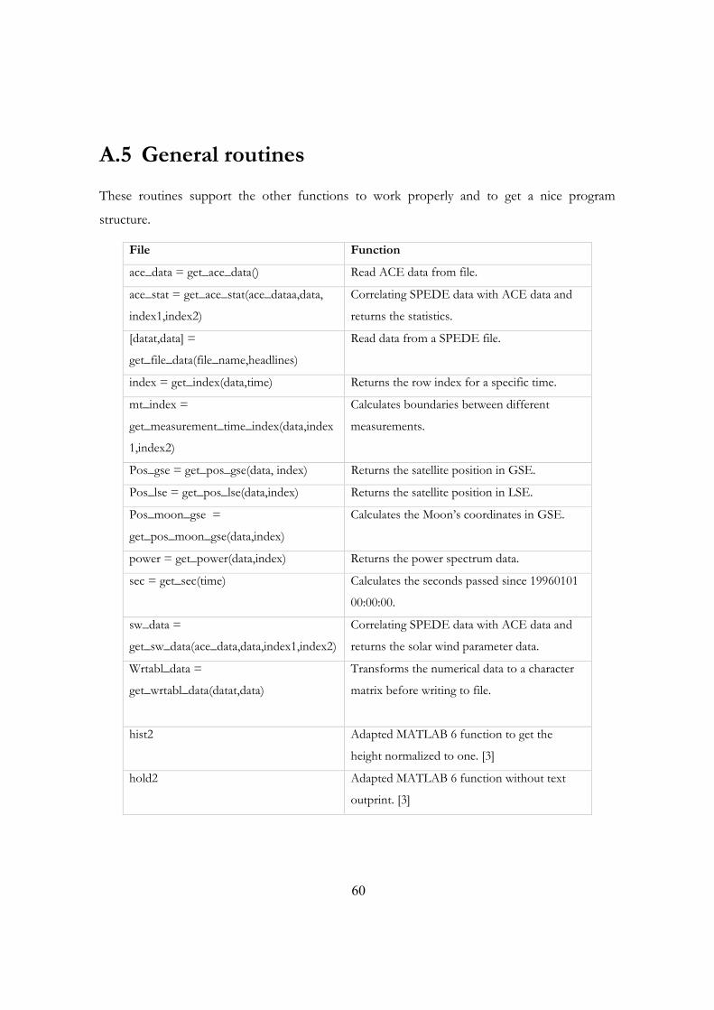
A.5 General routines These routines support the other functions to work properly and to get a nice program
structure.
File Function
ace_data = get_ace_data() Read ACE data from file.
ace_stat = get_ace_stat(ace_dataa,data,
index1,index2)
Correlating SPEDE data with ACE data and
returns the statistics.
[datat,data] =
get_file_data(file_name,headlines)
Read data from a SPEDE file.
index = get_index(data,time) Returns the row index for a specific time.
mt_index =
get_measurement_time_index(data,index
1,index2)
Calculates boundaries between different
measurements.
Pos_gse = get_pos_gse(data, index) Returns the satellite position in GSE.
Pos_lse = get_pos_lse(data,index) Returns the satellite position in LSE.
Pos_moon_gse =
get_pos_moon_gse(data,index)
Calculates the Moon’s coordinates in GSE.
power = get_power(data,index) Returns the power spectrum data.
sec = get_sec(time) Calculates the seconds passed since 19960101
00:00:00.
sw_data =
get_sw_data(ace_data,data,index1,index2)
Correlating SPEDE data with ACE data and
returns the solar wind parameter data.
Wrtabl_data =
get_wrtabl_data(datat,data)
Transforms the numerical data to a character
matrix before writing to file.
hist2 Adapted MATLAB 6 function to get the
height normalized to one. [3]
hold2 Adapted MATLAB 6 function without text
outprint. [3]

61
References [1] W.Schmidt, A.Mälkki & G.Racca (February 2, 2005). S1-SPE-MA-3001: SMART-1
SPEDE User Manual, pp. 9-14
[2] M.Genzer, W.Schmidt & A.Mälkki (May 10, 2005). S1-SPE-MA-3005: SMART1-
SPEDE To Planetary Science Archive Interface Control Document, pp. 5-6
[3] M.G.Kivelson & C.T.Russel (1995). Introduction to space physics, pp. 91-103, 169-172, 203-
206
[4] The Mathworks, Inc. (August 2, 2005). MATLAB Help: Version 7.1.0.246 (R14)
Service Pack 3
[5] The Wavelet Tutorial (1999). Polikar. (Electronic)
Availability: <http://users.rowan.edu/~polikar/WAVELETS/WTtutorial.html>.
(February 2, 2007)
[6] Wavelets and Signal Processing (2001). Kaplan. (Electronic)
Availability: <http://bearcave.com/misl/misl_tech/wavelets/>. (February 2, 2007)
[7] A.Schuck Jr. & J.O.Wisbeck (2003). QRS Detector Pre.processing Using the Complex Wavelet
Transform. Department of Electrical Engineering, Universidade Federal do Rio Grande
do Sul, Porto Alegre, RS, Brazil (Annual International Conference of the IEEE EMBS,
Cancun, Mexico, September 17-21, 2003)
[8] European Space Agency (2007). Availability:
<http://www.esa.int/esaSC/SEMI29374OD_0_spk.html>. (March 2, 2007)
[9] 1P.Trávníček, 1P.Hellinger, 2D.Schriver & 3S.D.Bale (2004). Structure of the lunar wake:
two-dimensional global hybrid simulations. 1Department of Space Physics, Institute of
Atmospheric Physics, Academy of the Czech Republic, 2Institute of Geophysics and
Planetary Physics, University of California Los Angeles, USA & 3Space Sciences
Laboratory and Department of Physics, University of California, Berkley, USA.
62
[10] Wavelets: “Beyond comparison”. D.L.Fugal Availability:
<http://www.aticourses.com/Wavelets%20-%20Beyond
%20Comparison%20by%20Lee%20Fugal.pdf>. (April 26, 2007)