Evaluation of SHRP Equipment - Rutgers University

Evaluation of SHRP Equipment (Non-Destructive Evaluation of Structures)

FINAL REPORT June 2001

Submitted by

P. N. Balaguru

Professor And

Dharm Bhatt, Mohamed Nazier Graduate Assistants

NJDOT Research Project Manager

Mr. Carey Younger

FHWA NJ 2001-12

In cooperation with

New Jersey Department of Transportation

Division of Research and Technology and

U.S. Department of Transportation Federal Highway Administration

Dept. of Civil & Environmental Engineering Center for Advanced Infrastructure & Transportation (CAIT)

Rutgers, The State University Piscataway, NJ 08854-8014

i

Disclaimer Statement

"The contents of this report reflect the views of the authors who are responsible for the facts and the

accuracy of the data presented herein. The contents do not necessarily reflect the official views or policies of the New Jersey Department of Transportation or the Federal Highway Administration. This report does not constitute

a standard, specification, or regulation."

The contents of this report reflect the views of the authors, Who are responsible for the facts and the accuracy of the

Information presented herein. This document is disseminated Under the sponsorship of the Department of Transportation, University Transportation Centers Program, in the interest of information exchange. The U.S. Government assumes no

liability for the contents or use thereof.

ii

1. Report No. 2. Government Accession No.

TECHNICAL REPORT STANDARD TITLE PAGE

3. Rec ip ient ’s Cata log No.

5 . Repor t Date

8. Performing Organization Report No.

6. Performing Organizat ion Code

4. Ti t le and Subt i t le

7. Author(s)

9. Performing Organization Name and Address 10. Work Unit No.

11. Contract or Grant No.

13. Type of Report and Period Covered

14. Sponsoring Agency Code

12. Sponsoring Agency Name and Address

15. Supplementary Notes

16. Abstract

17. Key Words

19. Security Classif (of this report)

Form DOT F 1700.7 (8-69)

20. Security Classif. (of this page)

18. Distr ibution Statement

21. No of Pages 22. Price

June 2001

CAIT/Rutgers

Final Report 02/01/2000 to 09/30/2001

FHWA 2001-12

New Jersey Department of Transportation CN 600 Trenton, NJ 08625

Federal Highway Administration U.S. Department of Transportation Washington, D.C.

Non-destructive evaluation of the condition of structures and possible solutions to improve the life of structures are being researched by a number of investigators. The results presented in this report focus on the performance of two instruments that are useful for rapid evaluation of the existing structures. The two instruments were developed as part of the SHRP program and have potential for wide spread use in the Transportation Infrastructure field. The Air Permeability Meter forces air in a pre-vacuumed concrete to estimate the permeability. The Corrosion Meter measures the corrosion potential and corrosion rate. For air permeability, tests were conducted on a new concrete surface, rough concrete, a newly painted surface and an old painted surface. A large number of readings were taken using two operators. The Corrosion Meter was used to measure corrosion rate and corrosion potential on instrumented bridges. The results were analyzed using statistical methods. The results and the analysis indicate that both instruments provide repeatable results. The evaluation form, which provides answers to specific questions, is presented in appendix A.

GECOR Corrosion Meter, Surface Air Permeability Meter, Corrosion Potential, Corrosion Rate,

Unclassified Unclassified

100

FHWA 2001-12

Dr. P.N. Balaguru, Dharm Bhatt and Mohamed Nazier

Evaluation of SHRP Equipment (Non-Destructive Evaluation of Structures)

iii

Acknowledgements The authors wish to express their appreciation to the New Jersey Department of Transportation for the allotment of funds making this research possible. Special thanks are extended to Mr. Carey Younger and Mr. Nicholas Vitillo of NJDOT for their support and extending the opportunity to participate in such a significant and extensive research program. Greatly appreciated was the co-operation and assistance of the graduate students Nicholas Wong, Anand Bhatt and Aseem Jaluria. Thanks to Edward Wass and Yubun Auyeung for their assistance in the laboratory.

iv

Table of Contents

Page Introduction 1 Objective 2 Description of Instruments 2 Test Program 7 Experimental Results and Analysis of Data: Permeability Meter 9 Experimental Results and Analysis of Data: Corrosion Meter 27 Conclusions 44 Recommendation 45 References 46 Appendix A 47 Appendix B 54

v

List of Figures Page Figure A Components of the GECOR 6 Corrosion Meter 2 Figure B Drawing of Concrete Surface Air Flow Permeability Meter 5 Figure 1 Livingston Freshly Painted Surface – Site No.1 11 Figure 2 Scatter Plot - Site No.1 12 Figure 3 Livingston Data – Site No.2 13 Figure 4 Scatter Plot – Site No. 2 14 Figure 5 Livingston Surface – Site No. 3 15 Figure 6 Scatter Plot – Site No. 3 16 Figure 7 East Brunswick Slab – Site No.4 17 Figure 8 Scatter Plot - Site No.4 18 Figure 9 College Avenue Data – Site No.5 19 Figure 10 Scatter Plot – Site No. 5 20 Figure 11 Livingston Front Porch – Site No. 6 21 Figure 12 Scatter Plot – Site No. 3 22 Figure 13 Operator 1 data 23 Figure 14 Scatter Plot Operator 1 24 Figure 15 Operator 2 Data 25 Figure 16 Scatter Plot Operator 2 26 Figure 17 Rt. 130 West Bound Data 29 Figure 18 Rt. 130 West Bound Data 30 Figure 19 North Main Street East Bound Data 31 Figure 20 North Main Street East Bound Data 32 Figure 21 North Main Street West Bound Data 33 Figure 22 North Main Street West Bound Data 34 Figure 23 Wycoff’s Bridge East Bound Data 35 Figure 24 Wycoff’s Bridge East Bound Data 36 Figure 25 Wycoff’s Bridge West Bound Data 37 Figure 26 Wycoff’s Bridge West Bound Data 38 Figure 27 Rt. 130 West Bound – Scatter Plot 39 Figure 28 North Main Street East Bound – Scatter Plot 40 Figure 29 North Main Street West Bound – Scatter Plot 41 Figure 30 Wycoff’s Bridge East Bound – Scatter Plot 42 Figure 31 Wycoff’s Bridge West Bound – Scatter Plot 43

vi

List of Tables Page Table 1 Interpretation of Corrosion Rate Data 4 Table 2 Interpretation of Half Cell (corrosion) Potential Readings 4 Table 3 Relative Concrete Permeability by Surface Air Flow 6 Table 4 Average and Standard deviation: Air Permeability Meter 10 Table 5 Average and Standard deviation: Corrosion Meter 28 Table 6 Livingston Freshly Painted Surface data – Site No.1 54 Table 7 Livingston data – Site No. 2 56 Table 8 Livingston Surface – Site No. 3 59 Table 9 East Brunswick Slab – Site No. 4 63 Table 10 College Avenue Data – Site No. 5 65 Table 11 Livingston Front Porch – Site No. 6 67 Table 12 Rt. 130 West Bound Cycle 1 69 Table 13 Rt. 130 West Bound Cycle 2 70 Table 14 Rt. 130 West Bound Cycle 3 71 Table 15 Rt. 130 West Bound Cycle 4 72 Table 16 Rt. 130 West Bound Cycle 5 73 Table 17 North Main Street East Bound Cycle 1 74 Table 18 North Main Street East Bound Cycle 2 75 Table 19 North Main Street East Bound Cycle 3 76 Table 20 North Main Street East Bound Cycle 4 77 Table 21 North Main Street East Bound Cycle 5 78 Table 22 North Main Street West Bound Cycle 1 79 Table 23 North Main Street West Bound Cycle 2 80 Table 24 North Main Street West Bound Cycle 3 81 Table 25 North Main Street West Bound Cycle 4 82 Table 26 North Main Street West Bound Cycle 5 83 Table 27 Wycoff’s Bridge East Bound Cycle 1 84 Table 28 Wycoff’s Bridge East Bound Cycle 2 85 Table 29 Wycoff’s Bridge East Bound Cycle 3 86 Table 30 Wycoff’s Bridge East Bound Cycle 4 87 Table 31 Wycoff’s Bridge East Bound Cycle 5 88 Table 32 Wycoff’s Bridge West Bound Cycle 1 89 Table 33 Wycoff’s Bridge West Bound Cycle 2 90 Table 34 Wycoff’s Bridge West Bound Cycle 3 91 Table 35 Wycoff’s Bridge West Bound Cycle 4 92 Table 36 Wycoff’s Bridge West Bound Cycle 5 93

1

ABSTRACT

Non-destructive evaluation of the condition of the structure and possible solutions to improve the life of the structure are being researched by a number of investigators. The results presented in this report focus on the performance of two instruments that are useful for rapid evaluation of the existing structures. The two instruments were developed as part of the SHRP program and have potential for wide spread use in the Transportation Infrastructure field. The Air Permeability Meter forces air in a pre-vacuumed concrete to estimate the permeability. The Corrosion Meter measures the corrosion potential and corrosion rate. For air permeability, tests were conducted on a new concrete surface, rough concrete, a newly painted surface and an old painted surface. A large number of readings were taken using two operators. The Corrosion Meter was used to measure corrosion rate and corrosion potential on instrumented bridges. The results were analyzed using statistical methods. The results and the analysis indicate that both instruments provide repeatable results. The evaluation form, which provides answers to specific questions, is presented in appendix A.

INTRODUCTION Repair and rehabilitation of transportation infrastructure is becoming a major part of the maintenance program. Two mechanisms that contribute to the deterioration are: corrosion of reinforcing steel in concrete and surface deterioration of concrete resulting in spalling and loss of cross section of structural elements. Good condition evaluation of the existing structure is a prerequisite for proper repair and rehabilitation. Non-destructive evaluation techniques provide excellent means to estimate the condition of structures without causing additional damage to structures. Results presented in this report deal with two NDT instruments. The first instrument measures surface permeability of concrete surface using forced airflow. The second instrument is used to measure the corrosion potential and corrosion rate. The primary objective of the study was to determine whether the instruments provide reproducible results. A large number of readings were taken using two operators and the results were analyzed to establish the repeatability.

2

OBJECTIVE The primary objective of the research was to evaluate the performance of corrosion rate and Air Permeability Meters. The major parameters were reproducibility and reliability. DESCRIPTION OF INSTRUMENT: Corrosion Instrument (Adapted from Manufacturer’s description) The GECOR 6 Corrosion Rate Meter provides valuable insight into the kinematics of the corrosion process. Based on a steady linear polarization technique it provides information on the rate of deterioration process. The meter monitors the electrochemical process of corrosion to determine the rate of deterioration. This nondestructive technique works by applying a small current to the reinforcing bar and measuring the change in the half-cell potential. The corrosion rate, corrosion potential and electrical resistance is provided by the corrosion rate meter. A photograph of the instrument is shown in Figure 1. More details can be found in Reference 1.

Figure A. Components of the GECOR 6 Corrosion Rate Meter

The GECOR 6 Corrosion Rate Meter has three major components, the rate meter and two separate sensors. Only the larger sensor was used during this project. The sensor is filled with a saturated Cu/CuSO4 solution for the test for half-cell potential. A wet sponge is used between the probe and the concrete surface. Long lengths of wire are also provided to connect the sensor to the rate meter and to connect the rate meter to the reinforcing bar mat of the bridge deck. This is a necessary step for the operation of the meter.

3

The procedure for the operation of the GECOR 6 Corrosion Rate Meter is as follows:

1. The device should not be operated at temperatures below 0° C (32° F) or above 50°

C (122° F). The relative humidity within the unit should not exceed 80%. 2. Use a reinforcing steel locator such as Pachometer to define the layout at the test

location. Mark the bar pattern on the concrete surface at the test location. 3. Place a wet sponge and the sensor over a single bar or over the point where the

bars intersect perpendicularly if the diameter of both bars is known. 4. Connect the appropriate lead to an exposed bar. The leads from the sensor and

exposed reinforcing steel are then connected to the GECOR device. 5. Turn on the unit. The program version appears on the display screen.

“LG-ECM-06 V2.0 GEOCISA 1993”

6. A help message appears on the screen momentarily. This message advises the operator to use the arrows for selecting an option and C.R. to activate an option. The various option are: • “CORROSION RATE MEASUREMENT” • “RELATIVE HUMIDITY AND TEMPERATURE” • “RESISTIVITY MEASUREMENT” • “EDIT MEASUREMENT PARAMETERS” • “DATE AND TIME CONTROL”

7. Select the option CORROSION RATE MEASUREMENT and press the C.R. key. 8. The screen prompts the user to input the area of steel. Calculate the area of steel

using the relationship, Area = 3.142 x D x 10.5 cm. D is the diameter of the bar in centimeters and 10.5 cm (4 in.) is the length of the bar confined by the guard ring. Key in the area to one decimal space. In case of an error, use the B key to delete the previous character. Press the C.R. key to enter the area.

9. The next screen displays: “ADJUSTING OFFSET, WAIT” No operator input is required at this stage. The meter measures the half-cell potential and then nulls it out to measure the potential shift created by the current applied from the sensor.

10. The next screen displays: “ Er mV OK” “ Vs mV OK” Er (ECORR) is the static half-cell potential versus Cse and is the difference in potential between the reference electrodes, which control the current confinement. Once the Er and the Vs values are displayed, no input is required from the operator.

11. The meter now calculates the optimum applied current ICE. This current is applied through the counter electrode at the final stage of the measurement. The optimum ICE value is displayed. No input is required from the operator.

12. The next screen displays the polarized potential values. No input is required from the operator.

4

13. The meter now calculates the “balance constant” in order to apply the correct current to the guard ring. It is displayed on the next screen. No input is required from the operator.

14. The meter now calculates the corrosion rate using the data collected from the sensor and input from the operator. The corrosion rate is displayed in µA/cm2. Associated parameters including corrosion potential, mV and electrical resistance kΩ can be viewed using the cursor keys.

15. Record the corrosion rate, corrosion potential and electrical resistance. 16. Press the B key to reset the meter for the next reading. The screen will return to

CORROSION RATE MEASUREMENT. Repeat the procedure for the next test location. The corrosion rate and corrosion potential data can be interpreted using the tables 1 and 2. These tables were taken from manufacturer’s literature.

Table 1 Interpretation of Corrosion Rate Data

ICORR (µA/cm2) Corrosion Condition Less than 0.1 Passive condition 0.1 to 0.5 Low to Moderate Corrosion 0.5 to 1.0 Moderate to High Corrosion Greater then 1.0 High Corrosion Table 2 Interpretation of Half Cell (Corrosion) Potential Readings Half Cell Potential (mV) Corrosion Activity -200 > 90% Probability of No Corrosion

Occurring -200 to –350 Corrosion Activity Uncertain <-350 90% Probability of Corrosion Occurring DESCRIPTION OF INSTRUMENT: Permeability Meter (Adapted from manufacturer’s description) The Concrete Surface Air Flow (SAF) Permeability Meter is a nondestructive technique designed to give an indication of the relative permeability of flat concrete surfaces. The SAF can be utilized to determine the permeability of concrete slabs, support members, bridge decks, and pavement (Manual for the Operation of a Surface Air Flow Field Permeability Indicator, 1994). The concrete permeability is based on airflow out of the concrete under an applied vacuum. The depth of measurement was determined to be approximately 0.5” below the concrete surface. A study between the relationships of SAF readings and of air and water permeability, determined that there is good correlation in the results (Scannell, 1996) Participant’s Workbook: FHWA – SHRP Showcase, (Scannell, 1996). The SAF should not be used as substitute for actual laboratory permeability testing. Cores tested under more standardized techniques will

5

provide a more accurate value for permeability due to the fact that the effects of surface texture and micro cracks have not been fully studied for the SAF. The SAF can determine permeability of both horizontal surfaces, by use of an integral suction foot, and vertical surfaces, by use of external remote head. The remote head was not used for this project. For transportability the device uses a rechargeable Ni-Cad battery. The suction foot is mounted using three centering springs to allow it to rotate and swivel in relation to the main body. The closed cell foam gasket is used between the foot and the testing surface to create an airtight seal. Two-foot pads are threaded into the suction foot so the operator can apply pressure to compress the gasket. The switches to open the solenoid and hold the current reading are located within easy reach at the base of the handles. Digital displays for the permeability readings and the time are located at the top of the device. A drawing of the instrument is shown in Figure2.

Figure B. Drawing of Concrete Surface Air Flow Permeability Meter

The procedure for the operation of the SAF on horizontal surfaces is as follows:

1. Remove the instrument from its case and install the two-foot pads. The footpads

should be screwed all the way into the tapped holes on the suction foot base and then backed out until the aluminum-checkered plates are pointed to the top of the machine.

2. Unfold the two handles by pushing the buttons on either end of the “T” handle lock pins, and removing them. When the handles are horizontal, the lock pins are needed to be inserted in the other holes ion the handle brackets to lock the handles in the extended positions.

3. Make sure all the switches are in the off position and the left handle switch in the RELEASE position. Set the elapsed time indicator to zero by pushing the RESET switch. Ensure that the directional valve switch is in the down position.

4. Charge the battery at least for eighteen hours before testing. 5. Unplug the charger and turn on the power switch, and observe that the digital

displays are activated. Turn ON the POWER switches. Wait ten minutes for the

6

device to warm up. The device should be tested before any field activities to make sure that it is operating correctly. To test the vacuum in a closed system, turn the pump in ON position. Wait thirty seconds. The readings should be stabilizing between 750 to 765 mmHg. To test the device as an open system, leave the PUMP ON and turn ON the solenoid switch. Wait thirty seconds. The readings should stabilize at a value of 29 to 31 SCCM.

6. To check the device on a reference plate, place the closed cell gasket on an impermeable metallic plate. Center the suction over the gasket.

7. Stand on the footpads. About half of the body weight should be placed on the footpads and the other half on the heels. This will compress the gasket and from an airtight seal.

8. Turn ON the PUMP. At this time both the flow and vacuum gages will display values and the elapsed time indicator will start. The vacuum should stabilize greater than 650 mmHg., vacuum. The flow will have a high initial value due to air in the lines, but will stabilize after about fifteen to twenty seconds.

9. Turn ON the solenoid switch. 10. When the elapsed time indicator reads 45 seconds, push the left handle switch to

the hold position to freeze the reading. Record the reading at this point. The vacuum should read greater than 50 mmHg, and the flow should be less than 1 SCCM (1 ml/min).

11. Turn OFF the vacuum pump, and the solenoid switch. Turn the switch on the left handle to the release position and push the reset button on the elapsed time indicator. The device is now ready to be moved to the next test spot.

12. Tests on actual concrete surfaces are performed in a manner identical to the initial check test. In some cases, however it may take longer than 45 seconds for the readings to stabilize. Surfaces should be dry, free of dirt or debris, and not cracked, grooved or textured.

The permeability of concrete greatly contributes to the corrosion potential of the embedded steel bas due to water and chloride penetration. The lower the permeability the more resistant the concrete is to chloride penetration. The relative concrete permeability readings provided by SAF can be categorized into low, moderate and high according to the flow rate (ml/min) as illustrated in the table below.

Table 3 Relative Concrete Permeability by Surface Air Flow

Air Flow Rate (ml/min) Relative Permeability Indicated 0 to 30 Low 30 to 80 Moderate 80> High

7

Test Program A large number of readings were taken using both instruments. The sites for readings were chosen to evaluate whether the instrument can distinguish between good and deteriorated surface, provide repeatable readings and consistent readings, and there is no variation between operators. Two operators took the readings at various times. Test Program: Corrosion Instrument Corrosion instrument was evaluated using five new bridge decks on Route 133 in New Jersey. Electrical connections were made to the top-reinforcing mat of each bridge deck before the placement of the concrete. Five connections were made to Route 130 West bound and four each on the remaining four bridges. A total of one hundred and five readings; twenty-five over Route 130 west bound, and twenty each at the other four bridge decks were taken for each cycle. One cycle represents five sets of readings at five locations. The data collection was repeated five times representing five cycles. Due to the use of epoxy coated reinforcing bars on the bridge deck over RT 130 West Bound, it was necessary to place uncoated reinforcing bars into the top mat. Short lengths of uncoated reinforcing bars were welded to the existing reinforcement. The ends were tapped to accept stainless steel nuts and bolts to attach underground copper feeder cables that were used to connect the meter to the reinforcement in the bridge deck. To ensure accurate readings, the connecting lengths of reinforcing bars were wire brushed to remove the existing corrosion. They were then coated with epoxy and spray painted to seal out moisture. The cables were passed through flexible steel conduits and into rain tight steel enclosure to protect them from the element and from possible tampering. A reinforcing steel locator was needed because locations of reinforcement and connections were not recorded before the placement of the concrete. Connections were observed during the placement of concrete and were tested after the concrete had hardened to check for broken connections. The connections were found to be working at all locations.

8

Test Program: Permeability Meter

The Air Permeability Meter was used at six different sites consisting of surfaces with good concrete, surfaces with damaged or rough concrete and a painted concrete surface.

About 500 readings were taken on each surface. These surfaces were chosen to verify that the machine will be able to distinguish between deteriorated and good surface and works well both on both good and deteriorated surfaces.

Following are the site descriptions where the Air Permeability Meter was used:

SITE NO. 1 This site, located at the Livingston Campus, Rutgers University, was a freshly painted surface. This surface had the potential for least permeability. SITE NO. 2 This site, located at the Livingston Campus, Rutgers University, was an old painted floor inside the building. The paint blistered off in few locations, but the concrete was in good condition. SITE NO. 3 This site, located at the Livingston Campus, Rutgers University, was an unpainted surface in good condition. SITE NO. 4 This site was a concrete floor in a residential building, located in East Brunswick. The floor was in good condition. SITE NO. 5 This site, located at the College Avenue Campus, Rutgers University, was parking deck with surface deterioration and therefore was more permeable than site 4.

SITE NO. 6 This site, located at the Livingston Campus front porch, Rutgers University, had considerably deteriorated concrete.

9

Experimental Results and Analysis of Data

The data collected was analyzed using a statistical software program called arena. The averages and the standard deviations were computed for all the data sets for both Air Permeability Meter and Corrosion Meter. The results are presented in Tables 4 and 5. Permeability Meter The results for the air permeability test are presented in the form of bar diagrams in Figures 1 to 12. The relation between the vacuum (mmHg) vs. flow (SCCM) is also presented to determine whether there is a relationship between these two parameters.

The equation for the regression line and the correlation coefficient, R² are also presented in these diagrams. The bar diagrams also show the variability of the air permeability in the concrete surface.

Figures 13 to 16 show the bar diagrams and scatter plots of the data taken during the tests by two different operators. The data show that the values taken by both operators seem to be similar, suggesting that the results are repeatable, between the operators. The averages and the standard deviations are presented in Table 4. The results presented in Table 4, the bar charts and the observations made during the collection of data lead to the following observations:

• The instrument can distinguish between good and deteriorated surfaces. Based on the surface conditions, flow (SCCM) had to increase from sites 1 to 6. The surface flow increased from about 4 for the best surface to 50 for the worst surface. The instrument provides more substantial information than visual inspection but not numerical numbers for permeability.

• The results do follow normal distribution for surfaces with low permeability such

as painted surfaces. Since the permeability varies considerably between test points of deteriorated surfaces, the variations do not follow normal curve.

• Based on the results obtained, the standard deviation increases with the increase

in average. But the increase is not proportional. Therefore the coefficient of variation is larger for surfaces with low permeability.

• Dependable relationship between vacuum and airflow does not exist.

10

Table 4 – Averages and Standard Deviations: Air Permeability Meter

Average Standard Deviation Site No. Name of the Site Vacuum

(mmHg) Flow

(SCCM) Vacuum (mmHg)

Flow (SCCM)

1 Livingston Campus, Freshly painted surface 779.1016 3.8067 .7901 1.3214

2 Livingston Campus, Old Painted Surface

785.5493 6.1022 2.7287 1.1025

3

Livingston Campus, Unpainted Surface

Good condition

793.9028 26.9182 1.5877 4.9644

4 East Brunswick,

Slab, Residential Building

775.7684 28.6269 4.2102 3.1949

5

College avenue Campus,

Parking Deck

720.8370 42.9351 23.4635 6.8451

6 Livingston Campus, Front porch 764.8377 52.8458 17.9312 4.9876

11

0

10

20

30

40

50

60

70

80

0-1 1-2 2-3 3-4 4-5 5-6 6-7

Flow (SCCM)

Figure 1 Livingston Freshly Painted Surface - Site No. 1

No.

of R

eadi

ngs

Series1

12

y = -1.1187x + 875.39

R2 = 0.4592

0

1

2

3

4

5

6

7

8

776.5 777 777.5 778 778.5 779 779.5 780 780.5 781 781.5

Vacuum (MMHg)

Figure 2 Livingston Freshly Painted - Site N0.1

Flo

w (S

CC

M)

Series1

Linear (Series1)

13

0

10

20

30

40

50

60

70

1-1.5 1.5-2 2-2.5 2.5-3 3-3.5 3.5-4 4-4.5 4.5-5 5-5.5 5.5-6 6-6.5 6.5-7 7-7.5 7.5-8 8-8.5 8.5-9 9-9.5

Flow (SCCM)

Figure 3 Livingston Data - Site No. 2

Num

ber

of R

eadi

ngs

Series1

14

y = -0.656x + 519.85R2 = 0.1758

0

1

2

3

4

5

6

7

8

9

10

779 780 781 782 783 784 785 786

Vacuum (MMHg)

Figure 4 Livingston Data - Site No.2

Flow

(SC

CM

)

Series1Linear (Series1)

15

0

20

40

60

80

100

120

15-17 17-19 19-21 21-23 23-25 25-27 27-29 29-31 31-33 33-35 35-37 37-39 39-41 41-43 43-45 45-47 47-49 49-51 51-53 53-55 55-57 57-59

Flow (SCCM)


No

. of R

ead

ing

s

Series1

16

y = -1.4772x + 1199.7R2 = 0.2232

0

10

20

30

40

50

60

70

780 782 784 786 788 790 792 794 796 798Vacuum (MMHg)


Flo

w (S

CC

M)

Series1

Linear (Series1)

17

0

5

10

15

20

25

30

23-24

24-25

25-26

26-27

27-28

28-29

29-30

30-31

31-32

32-33

33-34

34-35

35-36

36-37

37-38

38-39

39-40

40-41

41-42

42-43

43-44

44-45

45-46

46-47

Flow (SCCM)

Figure 7 East Brunswick Slab - Site No. 4

No

. of R

ead

ing

s

Series1

18

y = -0.307x + 266.76

R2 = 0.1315

0

5

10

15

20

25

30

35

40

45

50

766 768 770 772 774 776 778 780 782 784 786

Vacuum (MMHg)

Figure 8 East Brunswick Slab - Site No. 4

Flo

w (S

CC

M)

Series1

Linear (Series1)

19

0

2

4

6

8

10

12

32-34 34-36 36-38 38-40 40-42 42-44 44-46 46-48 48-50 50-52 52-54 54-56 56-58

Flow (SCCM)

Figure 9 College Ave Data - Site No. 5

Num

ber

of R

eadi

ngs

Series1

20

y = 0.2346x - 126.2

R2 = 0.6468

0

10

20

30

40

50

60

70

0 100 200 300 400 500 600 700 800 900

Vacuum (MMHg)

Figure 10 College Ave Data - Site No. 5

Flo

w (S

CC

M)

Series1

Linear (Series1)

21

0

5

10

15

20

25

30

35

40

45

41-43 43-45 45-47 47-49 49-51 51-53 53-55 55-57 57-59 59-61 61-62

Flow (SCCM)

Figure 11 Livingston Front Porch - Site No. 6

Num

ber

of R

eadi

ngs

Series1

22

y = 0.0589x + 7.8369R2 = 0.0449

0

10

20

30

40

50

60

70

710 720 730 740 750 760 770 780 790

Vacuum (mmHg)

Figure 12 Livingston Front Porch - Site No. 6

Flo

w (S

CC

M)

Series1

Linear (Series1)

23

0

10

20

30

40

50

60

70

1-1.5 1.5-2 2-2.5 2.5-3 3-3.5 3.5-4 4-4.5 4.5-5 5-5.5 5.5-6 6-6.5 6.5-7 7-7.5 7.5-8 8-8.5 8.5-9 9-9.5

Flow (SCCM)

Figure 13 Livingston Data - Operator 1

Num

ber

of R

eadi

ngs

Series1

24

y = -0.656x + 519.85R2 = 0.1758

0

1

2

3

4

5

6

7

8

9

10

779 780 781 782 783 784 785 786

Vacuum (MMHg)

Figure 14 Livingston Data (Operator 1)

Flow

(SC

CM

)

Series1Linear (Series1)

25

0

10

20

30

40

50

60

70

3-3.5 3.5-4 4-4.5 4.5-5 5-5.5 5.5-6 6-6.5 6.5-7 7-7.5 7.5-8 8-8.5 8.5-9

Flow (SCCM)


Nu

mb

er o

f rea

din

gs

Series1

26

y = -0.1569x + 129.82R2 = 0.0482

0

1

2

3

4

5

6

7

8

9

10

785 786 787 788 789 790 791 792

Vacuum (MMHg)


Flo

w (S

CC

M)

Series1

Linear (Series1)

27

Corrosion Meter The results for the Corrosion Instrument test are presented in Figures 17-31. The figures show the frequency distribution of Corrosion Rate, Corrosion Potential, and the relationship between the two for the five sites. Regression equations and correlation coefficients, R² are also presented for the relationships between Corrosion rate and Corrosion Potential, Figures 27 to 31. The averages and the standard deviations are presented in Table 5. The results presented in Table 5, the bar charts and the observations made during the collection of data lead to the following observations:

• The instrument provides repeatable and consistent readings. Note that variation should be expected across the deck area because the corrosion levels could be different.

• Since all the decks are new, it was expected that the readings should be in a small range and the instrument

confirms this expectation.

• Both the corrosion rate and corrosion potential do not follow any trend. This should be expected because there is very little corrosion activity and the values are real random numbers produced by initial rust.

• There is no relationship between corrosion rate and corrosion potential. Low corrosion rate is the reason for this

observation

• The standard deviations are very high compared to averages because the corrosion level is very low and hence the noise is high.

• The instrument can be operated without any difficulty both in the laboratory and in the field. The authors

recommend the use of this instrument for corrosion measurements.

28

Table 5 – Average and Standard Deviation: Corrosion Meter

Average Standard Deviation

Site No. Name of the Site

Corrosion Rate,

uA/cm²

Corrosion Potential,

mV

Corrosion Rate,

uA/cm²

Corrosion Potential,

mV

1 Rt. 130 West bound 0.1645 30.40 0.1008 35.80

2 North Main Street Eastbound 0.2329 -77.70 0.1959 47.14

3 North Main Street Westbound 0.1733 -151.62 0.0650 63.23

4 Wycoff Eastbound 0.1793 -70.94 0.1307 49.16

5 Wycoff Westbound 0.1561 -198.57 0.1207 1181.23

29

0

0.1

0.2

0.3

0.4

0.5

0.6

0.7

0.8

0.91 5 9 13 17 21 25 29 33 37 41 45 49 53 57 61 65 69 73 77 81 85 89 93 97 101

105

109

113

117

121

125

Number of ReadingsFigure 17 Corrosion Rate: Rt. 130 West Bound Data

Co

rro

sio

n R

ate

(uA

/cm

2)

Series1

30

-100

-50

0

50

100

150

1 5 9 13 17 21 25 29 33 37 41 45 49 53 57 61 65 69 73 77 81 85 89 93 97 101

105

109

113

117

121

125

Number of Readings

Figure 18 Corrosion Potential: Rt. 130 West bound Data

Co

rro

sio

n P

ote

nti

al (m

V)

Series1

31

0

0.1

0.2

0.3

0.4

0.5

0.6

0.7

0.8

0.9

11 4 7 10 13 16 19 22 25 28 31 34 37 40 43 46 49 52 55 58 61 64 67 70 73 76 79 82 85 88 91 94 97 100

Number of Readings

Figure 19 Corrosion Rate: North Main Street East Bound Data

Co

rro

sio

n R

ate

(uA

/cm

2)

Series1

32

-200

-180

-160

-140

-120

-100

-80

-60

-40

-20

01 4 7 10 13 16 19 22 25 28 31 34 37 40 43 46 49 52 55 58 61 64 67 70 73 76 79 82 85 88 91 94 97 100

Number of Readings

Figure 20 Corrosion Potential: North Main Street East Bound Data

Co

rro

sio

n P

ote

nti

al (m

V)

Series1

33

0

0.05

0.1

0.15

0.2

0.25

0.3

0.35

0.4

0.45

1 4 7 10 13 16 19 22 25 28 31 34 37 40 43 46 49 52 55 58 61 64 67 70 73 76 79 82 85 88 91 94 97 100

Number of Readings

Figure 21 Corrosion Rate: North Main Street West Bound Data

Co

rro

sio

n R

ate

(uA

/cm

2)

Series1

34

-300

-250

-200

-150

-100

-50

0

1 4 7 10 13 16 19 22 25 28 31 34 37 40 43 46 49 52 55 58 61 64 67 70 73 76 79 82 85 88 91 94 97 100

Number of Readings

Figure 22 Corrosion Potential: North Main Street West Bound Data

Cor

rosi

on P

oten

tial (

mV

)

Series1

35

0

0.1

0.2

0.3

0.4

0.5

0.6

0.7

0.8

1 4 7 10 13 16 19 22 25 28 31 34 37 40 43 46 49 52 55 58 61 64 67 70 73 76 79 82 85 88 91 94 97 100

Number of Readings

Figure 23 Corrosion Rate: Wycoff's Bridge East Bound Data

Cor

rosi

on R

ate

(uA

/cm

2)

Series1

36

-200

-150

-100

-50

0

50

1 4 7 10 13 16 19 22 25 28 31 34 37 40 43 46 49 52 55 58 61 64 67 70 73 76 79 82 85 88 91 94 97 100

Number of Readings

Figure 24 Corrosion Potential: Wycoff's Bridge East Bound Data

Co

rro

sio

n P

ote

nti

al (m

V)

Series1

37

0

0.1

0.2

0.3

0.4

0.5

0.6

1 4 7 10 13 16 19 22 25 28 31 34 37 40 43 46 49 52 55 58 61 64 67 70 73 76 79 82 85 88 91 94 97 100

Number of Readings

Figure 25 Corrosion Rate: Wycoff's Bridge West Bound Data

Co

rro

sio

n R

ate

(uA

/cm

2)

Series1

38

-250

-200

-150

-100

-50

0

50

1 4 7 10 13 16 19 22 25 28 31 34 37 40 43 46 49 52 55 58 61 64 67 70 73 76 79 82 85 88 91 94 97 100

Number of Readings

Figure 26 Corrosion Potential: Wycoff's Bridge West Bound Data

Co

rro

sio

n P

ote

nti

al (m

V)

Series1

39

y = -72.406x + 45.639R2 = 0.0428

-100

-50

0

50

100

150

0 0.1 0.2 0.3 0.4 0.5 0.6 0.7 0.8 0.9

Corrosion Rate (uA/cm2)

Figure 27 Corrosion Potential vs. Corrosion Rate: Rt. 130 West Bound - Scatter Plot

Co

rro

sio

n P

ote

nti

al (m

V)

Series1

Linear (Series1)

40

y = -163.55x - 39.246

R2 = 0.4602-200

-180

-160

-140

-120

-100

-80

-60

-40

-20

00 0.1 0.2 0.3 0.4 0.5 0.6 0.7 0.8 0.9 1


Figure 28 Corrosion Potential vs. Corrosion Rate: North Main Street East Bound - Scatter Plot

Co

rro

sio

n P

ote

nti

al (m

V)

Series1

Linear (Series1)

41

y = 332x - 211.78

R2 = 0.1448

-300

-250

-200

-150

-100

-50

00 0.05 0.1 0.15 0.2 0.25 0.3 0.35 0.4 0.45


Figure 29 Corrosion potentail vs. Corrosion Rate: North Main Street West Bound - Scatter Plot

Co

rro

sio

n P

ote

nti

al (m

V)

Series1

Linear (Series1)

42

y = -150.49x - 40.249R2 = 0.1779

-200

-150

-100

-50

0

50

0 0.1 0.2 0.3 0.4 0.5 0.6 0.7 0.8


Figure 30 Corrosion Potential vs. Corrosion Rate: Wycoff's Bridge East Bound - Scatter Plot

Co

rro

sio

n P

ote

nti

al (m

V)

Series1

Linear (Series1)

43

y = -213.23x - 57.337R2 = 0.3023

-250

-200

-150

-100

-50

0

50

0 0.1 0.2 0.3 0.4 0.5 0.6


Figure 31 Corrosion Potential vs. Corrosion Rate: Wycoff's Bridge West Bound - Scatter Plot

Co

rro

sio

n P

ote

nti

al (m

V)

Series1

Linear (Series1)

44

CONCLUSIONS

Based on the experimental results and their analysis and observations made during the testing the following conclusions can be drawn. Both instruments are easy to operate and the instructions provided by the manufacturers are adequate for operating the instruments.

Permeability Meter

• The instrument can distinguish between good and deteriorated surfaces. Based

on the surface conditions, flow (SCCM) had to increase from sites 1 to 6. The surface flow increased from about 4 for the best surface to 50 for the worst surface. Note that the instrument is not designed to provide actual permeability numbers.

• As expected, the distribution was a bell shape curve or normal curve for best

surface having less scatter or standard deviation.

• Based on the results obtained, both the average value and the standard deviation should be used to determine the condition of the surface.

• Dependable relationship between vacuum and airflow does not exist.

Corrosion Meter • The instrument provides consistent results and variations. Note that variation

should be expected across the deck area. • Since all the decks are new, it was expected that the readings should be in a

small range and the instrument confirms this expectation. • Both the corrosion rate and corrosion potential do not follow any trend. This

should be expected because there is very little corrosion activity and the values are real random numbers produced by initial rust.

• There is no relationship between corrosion rate and corrosion potential. The

authors believe that since the corrosion levels were very low, there is a lack of relationship between corrosion potential and corrosion rate.

45

RECOMMENDATIONS Based on the results obtained and the experience of the operators, the author recommends the use of both the instruments for measuring permeability and corrosion. The results from Air Permeability Meter should be used only as a semi quantitative measure.

46

References

1. Manual for the Operation of a Surface Air Flow Field Permeability Indicator, Texas Research Institute Austin, Inc., Austin Texas, June 1994

2. 3. Broomfield, John P., Corrosion of Steel in Concrete: Understanding

Investigation and Repair, E & FN Spoon, London, UK 1997

4. Scannel, William T. Participant’s Workbook: FHWA-SHRP Showcase, U.S. Department of Transportation, Concorr Inc., Ashburn, July, 1996

5. Sennour, M. L, Carrasquillo, R. L., The Effects of Chemical and Mineral

Admixtures on the Corrosion of Steel in Concrete, University of Texas, Austin, Texas 1994

47

Appendix A This appendix presents the completed survey forms distributed through SHRP program.

48

49

50

51

52

53

54

Appendix B This appendix presents the data obtained at the various locations for both Air Permeability and Corrosion Meters. Air permeability data tables Table 6: Livingston Freshly Painted Surface – Site No. 1

Vacuum (mmHg)

Flow (SCCM)

Vacuum (mmHg)

Flow (SCCM)

Vacuum (mmHg)

Flow (SCCM)

Vacuum (mmHg)

Flow (SCCM)

Vacuum (mmHg)

Flow (SCCM)

776.9 5.1 778.4 4.33 778.9 4.98 779.1 2.85 779.5 3.77776.9 5.4 778.4 5.09 778.9 3.55 779.1 4.27 779.5 3.06776.9 5.4 778.4 4.27 778.9 5.94 779.1 3.98 779.5 3.89777.2 4.28 778.4 5.09 778.9 4.32 779.1 4.93 779.5 3.86777.2 4.28 778.5 4.08 778.9 4.6 779.1 3.9 779.6 1.23777.3 4.73 778.5 3.74 778.9 4.96 779.1 6.31 779.6 1.77777.8 5.25 778.5 3.86 778.9 5.22 779.1 3.65 779.6 2.89777.8 4.59 778.5 3.36 778.9 5.29 779.1 2.59 779.6 2.52777.8 4.47 778.5 4.13 778.9 4.98 779.1 2.85 779.6 2.67777.8 5.98 778.5 5.13 778.9 4.92 779.1 4.93 779.6 3.44777.8 5.92 778.5 4.78 778.9 2.98 779.2 3.74 779.6 4.21777.8 4.01 778.5 4.13 778.9 3.42 779.2 2.55 779.7 2.3777.8 4.14 778.5 5.44 778.9 3.96 779.2 2.45 779.7 0.89777.9 3.4 778.5 4.28 778.9 3.94 779.2 1.6 779.7 1.98777.9 4.2 778.6 5.91 778.9 3.81 779.2 3.76 779.7 3.45

778 6.54 778.6 4.16 778.9 4 779.2 4.22 779.7 3.65778 4.51 778.6 5.07 778.9 4.99 779.2 3.27 779.7 4.02778 3.15 778.6 5.24 778.9 2.59 779.2 3.53 779.7 5.49778 3.46 778.6 5.09 778.9 5.4 779.2 3.27 779.8 3.3778 3.46 778.6 4.33 779 3.64 779.2 3.53 779.8 1.4

778.1 4.22 778.6 5.41 779 3.54 779.3 1.31 779.8 2.57778.1 4.71 778.6 5.37 779 3.71 779.3 1.19 779.8 3.06778.1 6.61 778.6 5.74 779 3.8 779.3 2.13 779.8 3.19778.1 4.12 778.6 5.09 779 5.69 779.3 3.79 779.9 1.02778.1 5.09 778.6 4.33 779 5.26 779.3 3.77 779.9 4.84778.1 4.9 778.6 5.09 779 4.36 779.3 4.08 780 3.89778.1 3.93 778.7 5.81 779 3.18 779.3 4.69 780 2.42778.2 5.86 778.7 5.36 779 3.75 779.3 4.12 780 2.89778.2 5.22 778.7 5.98 779 3.72 779.3 4.38 780 1.76

55

778.2 4.6 778.7 4.58 779 3.89 779.3 3.85 780 1.27778.2 6.35 778.7 3.62 779 5.43 779.3 3.66 780 1.99778.2 4.6 778.7 3.92 779 5.26 779.3 4.25 780 2.75778.2 6.35 778.7 3.78 779.1 1.97 779.3 3.95 780 2.39778.2 4.4 778.7 5.44 779.1 2.81 779.3 4.51 780 4.07778.3 4.66 778.7 5.44 779.1 2.68 779.3 3.95 780 3.89778.3 4.35 778.7 3.95 779.1 3.1 779.4 4.77 780.1 3.59778.3 4.3 778.8 4.95 779.1 5.06 779.4 3.61 780.1 3.43778.3 5.33 778.8 4.11 779.1 4.52 779.4 4.14 780.1 2.07778.3 4.07 778.8 4.9 779.1 3.7 779.4 4.73 780.1 2.04778.3 5.33 778.8 5.12 779.1 3.62 779.4 4.14 780.1 2.55778.4 6.36 778.8 4.64 779.1 3.27 779.4 2.85 780.1 2.22778.4 6.78 778.8 5.05 779.1 4.11 779.5 1.96 780.1 1.13778.4 5.91 778.8 4.64 779.1 3.55 779.5 1.7 780.1 2.93778.8 5.09 779.1 3.81 779.5 1.52 780.1 2.54 778.8 4.33 779.1 3.65 779.5 3.19 780.1 4.12 778.9 1.66 779.1 2.59 779.5 4.06 780.2 3.15 780.2 2.94 780.2 2.77 780.3 2.04 780.3 2.33 780.4 2.27 780.4 2.07 780.5 2.18 780.5 2.16 780.6 0.44 780.6 1.93 780.6 2.07 780.6 2.85 780.6 2.75 780.6 2.25 780.6 0.44 780.6 1.93 780.8 1.27 780.8 2.82 780.8 1.82 780.8 1.02 780.8 1.27 780.9 1.86 781.1 1.41

56

Table 7: Livingston data – Site No. 2

Vacuum (mmHg)

Flow (SCCM)

Vacuum (mmHg)

Flow (SCCM)

Vacuum (mmHg)

Flow (SCCM)

Vacuum (mmHg)

Flow (SCCM)

Vacuum (mmHg)

Flow (SCCM)

781 55.14 791.8 23.94 792.4 22.63 792.4 21.58 793.7 28.15

787.4 39.55 791.8 25.94 792.4 24.93 792.4 22.96 793.8 27.19787.6 57.64 791.8 26.51 792.4 31.11 792.4 28.01 793.8 31.43788.4 39.15 791.8 26.96 792.5 23.23 792.4 30.4 793.8 32.06788.6 36.82 791.8 28.51 792.5 24.45 792.4 31.11 793.8 23.17788.8 36.67 791.8 28.51 792.5 26.01 792.4 20.92 793.8 23.17788.9 33.01 791.8 30.63 792.5 26.01 793.2 24.49 793.8 25.43789.1 33.5 791.9 27.62 792.5 18.73 793.3 21.08 793.8 27.19789.4 36.25 791.9 30.29 792.5 22.1 793.3 26.82 793.8 31.43789.6 33.97 791.9 22.6 792.5 24.44 793.3 34.05 793.8 32.06

790 42.24 791.9 23.44 792.6 21.01 793.3 34.05 793.8 32.06790.3 43.81 791.9 24.42 792.6 21.69 793.3 34.05 793.9 21.5790.4 40.72 791.9 24.66 792.6 26.37 793.4 27.26 793.9 24.46790.5 31.64 791.9 26.17 792.6 27.11 793.4 27.69 793.9 24.91790.5 37.2 791.9 26.17 792.6 18.27 793.4 34.88 793.9 26.61790.5 38.13 791.9 26.41 792.6 18.97 793.4 23.02 793.9 27.49790.6 46.84 792 21.64 792.6 22.93 793.4 23.02 793.9 28.15790.7 31.26 792 22.4 792.7 21.15 793.4 27.69 793.9 36.8790.8 31.34 792 22.66 792.7 22.58 793.5 25 793.9 24.91790.8 33.39 792 24.15 792.7 26.99 793.5 25.7 793.9 26.16791.1 32.04 792 25.88 792.7 34.02 793.5 23.18 793.9 26.61791.2 24.88 792 26.17 792.7 36.32 793.5 25.7 793.9 27.49791.2 26.33 792.1 26.43 792.7 36.32 793.6 24.22 793.9 27.49791.2 28.75 792.1 21.5 792.7 36.32 793.6 24.81 793.9 28.15791.3 35.56 792.1 22.52 792.8 21.44 793.6 25.27 793.9 29.68791.3 42.93 792.1 22.52 792.9 34.18 793.6 27.13 793.9 29.68791.3 24.19 792.1 22.52 792.9 21.38 793.6 28.42 794 21.16791.4 31.7 792.1 22.56 792.9 34.18 793.6 28.93 794 24.81791.4 33.66 792.1 32.52 793 21.82 793.6 29.21 794 25.05791.4 48.66 792.2 42.88 793 26.91 793.6 29.65 794 26.85791.4 32.06 792.2 20.23 793 20.22 793.6 37.45 794 28.77791.5 25.09 792.2 21.28 793 21.63 793.6 25.27 794 28.77791.6 34.7 792.2 25.97 793 26.91 793.6 25.27 794 29.14791.6 28.39 792.3 22.58 793 26.91 793.6 28.42 794 29.14791.6 28.39 792.3 23.29 793.1 41.54 793.6 28.42 794 32.95

57

791.7 30.44 792.3 23.61 793.1 21.78 793.6 29.21 794 36.39791.7 23.69 792.3 21.64 793.1 41.54 793.6 29.65 794 24.26791.8 30.63 792.3 22.18 793.2 23.53 793.6 29.65 794 24.81791.8 41.65 792.3 25.04 793.2 33.82 793.7 30.58 794 24.81791.8 21.98 792.3 25.77 793.2 37.45 793.7 34.62 794 25.05

793.7 36.21 794 25.05794.1 25.36 794 26.85 794.6 24.83 794.5 29.77 795 27.49794.1 25.98 794 26.85 794.6 25.74 794.5 30.37 795 27.97794.1 26.03 794 28.77 794.6 26.22 794.5 30.75 795 27.97794.1 26.03 794 28.77 794.6 26.22 794.5 22.57 795 23.42794.1 27.02 794 32.95 794.6 27.73 794.5 22.7 795 23.42794.1 27.29 794 36.39 794.6 27.73 794.5 24.85 795 24.12794.1 27.29 794.1 21.74 794.6 27.98 794.5 24.85 795 24.66794.1 27.79 794.1 23.06 794.6 21.31 794.5 24.85 795 26.36794.1 27.79 794.1 24.81 794.6 21.79 794.5 25.46 795 27.49794.1 27.79 794.1 24.82 794.6 21.79 794.5 25.46 795.1 15.86794.1 30.05 794.1 25.36 794.6 23.39 794.5 25.63 795.1 19.8794.1 30.13 794.1 25.98 794.6 23.39 794.5 25.63 795.1 24.12794.1 31.38 794.1 26.03 794.6 23.77 794.5 26.82 795.1 25.82794.1 31.38 794.1 30.05 794.6 23.77 794.5 26.82 795.1 26.4794.1 31.59 794.1 30.13 794.6 23.89 794.5 27.13 795.1 26.4794.2 27.34 794.1 31.38 794.6 24.83 794.5 27.13 795.1 27794.2 27.34 794.1 31.59 794.6 24.83 794.5 27.85 795.1 27.03794.2 32.26 794.1 24.7 794.6 25.74 794.5 28.34 795.1 27.03794.2 25.8 794.1 24.7 794.6 25.74 794.6 21.31 795.1 27.86794.2 25.8 794.1 24.81 794.6 26.22 794.6 21.79 795.1 28.29794.2 26.92 794.1 24.81 794.6 27.73 794.6 22.11 795.1 28.51794.2 26.92 794.1 24.82 794.6 27.98 794.6 22.7 795.1 28.66794.2 26.92 794.1 25.36 794.7 21.86 794.6 23.89 795.1 15.93794.2 29.77 794.4 23.74 794.7 22.44 794.8 27.17 795.1 19.8794.3 22.41 794.4 25.8 794.7 23.92 794.8 28.54 795.1 19.8794.3 23.33 794.4 25.8 794.7 28.91 794.8 29.54 795.1 25.82794.3 25.51 794.4 26.75 794.7 29.84 794.8 29.54 795.1 25.82794.3 26.44 794.4 27.48 794.7 29.84 794.8 19.81 795.1 27794.3 26.44 794.4 30.12 794.7 32.16 794.8 20.91 795.1 27.86794.3 27.5 794.4 38.19 794.7 32.16 794.8 28.54 795.1 27.86794.3 27.7 794.4 21.31 794.7 21.86 794.8 28.54 795.1 28.29794.3 28.76 794.4 23.74 794.7 23.92 794.9 17.11 795.1 28.59794.3 28.76 794.4 25.8 794.7 23.92 794.9 17.91 795.2 20.91794.3 32.98 794.4 25.8 794.7 25.1 794.9 22.81 795.2 21.62794.3 33.04 794.4 26.75 794.7 28.91 794.9 25.1 795.2 21.62794.3 22.41 794.4 27.48 794.7 28.91 794.9 26.7 795.2 21.62794.3 23.33 794.4 27.48 794.8 19.81 794.9 27.43 795.2 24.17794.3 24.57 794.4 27.48 794.8 20.91 794.9 27.43 795.2 24.17794.3 25.51 794.5 22.57 794.8 24.39 794.9 17.81 795.2 24.77794.3 25.51 794.5 22.7 794.8 24.39 794.9 25.1 795.2 24.77

58

794.3 25.51 794.5 25.46 794.8 24.39 795 23.42 795.2 28.37794.3 27.03 794.5 25.63 794.8 26.8 795 24.66 795.2 30.12794.3 27.7 794.5 26.82 794.8 26.8 795 24.66 795.2 20.91794.3 28.76 794.5 27.13 794.8 26.82 795 26.36 795.2 20.91794.3 29.57 794.5 27.85 794.8 26.82 795 27.36 795.2 24.17794.4 21.31 794.5 27.85 794.8 27.17 795 27.36 795.3 22.44795.6 25.33 795.3 25.7 795.8 25.9 796.3 26.93 795.6 25.53 795.3 25.7 795.8 25.9 796.7 19.77 795.6 25.83 795.3 26.93 795.8 27.2 796.7 19.77 795.6 27.23 795.3 28.93 795.9 24.77 795.6 22.62 795.6 32.86 795.3 28.93 795.9 24.77 795.6 24.84 795.6 22.62 795.4 24.08 796 18.87795.6 24.84 795.4 24.08 796 24.87795.6 25.83 795.4 26.41 796 18.87795.6 27.23 795.4 27.25 796 24.81795.7 24.6 795.4 27.25 796.2 21.82795.7 28.34 795.4 27.61 796.2 23.1795.7 28.34 795.4 30.21 796.2 23.1795.8 23.74 795.5 22.49 796.3 21.68795.8 23.74 795.5 26.03 796.3 21.93795.8 25.9 795.5 27.21 796.3 22.08795.8 27.09 795.5 27.21 796.3 24.55795.8 27.09 795.5 31.06 796.3 26.93795.8 27.2 795.5 32.47 796.3 21.68795.8 35.66 795.5 22.49 796.3 21.93795.8 22.87 795.5 26.03 796.3 22.08795.8 22.87 795.5 31.06 796.3 24.55

59

Table 8: Livingston Surface – Site No. 3

Vacuum (mmHg)

Flow (SCCM)

Vacuum (mmHg)

Flow (SCCM)

Vacuum (mmHg)

Flow (SCCM)

Vacuum (mmHg)

Flow (SCCM)

Vacuum (mmHg)

Flow (SCCM)

780.1 7.63 782.7 4.21 783 6.63 783.4 5.28 783.7 3.43 780.9 8.31 782.7 4.55 783 6.67 783.4 5.46 783.7 4.16 781.4 7.16 782.7 5.65 783 6.68 783.4 5.68 783.7 5.05 781.4 8.35 782.7 6.14 783 6.71 783.4 5.88 783.7 5.69 781.6 4.28 782.7 6.21 783 6.72 783.4 6.17 783.7 5.69 781.7 7.66 782.7 6.27 783 6.77 783.4 6.45 783.7 5.78 781.8 3.32 782.7 6.43 783 6.87 783.4 6.54 783.7 5.91 781.9 5.01 782.7 6.5 783 6.96 783.4 6.65 783.7 6.48 781.9 6.01 782.7 6.6 783 7.47 783.4 6.72 783.7 6.6

782 6.69 782.7 6.92 783 7.52 783.4 6.74 783.7 6.7 782 6.7 782.7 7.58 783 7.56 783.4 6.9 783.8 5.06 782 6.98 782.8 5.16 783 7.83 783.4 7.38 783.8 5.34 782 7.56 782.8 5.38 783.1 3.53 783.4 8.62 783.8 5.56 782 7.83 782.8 5.43 783.1 4.74 783.5 4.52 783.8 5.66 782 8.07 782.8 5.95 783.1 5.07 783.5 4.94 783.8 5.78 782 8.65 782.8 6.48 783.1 5.1 783.5 5.06 783.8 6.26 782 8.72 782.8 6.66 783.1 5.45 783.5 5.31 783.8 6.92 782 9.12 782.8 6.78 783.1 6.05 783.5 5.67 783.8 7.23

782.1 6.36 782.8 6.79 783.1 6.05 783.5 5.84 783.8 7.29 782.1 6.4 782.8 7.15 783.1 6.1 783.5 5.88 783.9 2.09 782.1 6.48 782.9 5.79 783.1 6.12 783.5 6.08 783.9 4.86 782.1 6.49 782.9 6.29 783.1 6.43 783.5 6.1 783.9 5.5 782.1 6.52 782.9 6.52 783.1 6.45 783.5 6.14 783.9 6.53 782.1 6.59 782.9 6.6 783.1 6.65 783.5 6.27 783.9 6.9 782.1 7.92 782.9 6.6 783.1 6.85 783.5 6.42 783.9 6.97 782.2 5.67 782.9 6.66 783.1 7.04 783.5 6.46 783.9 7.43 782.2 6.28 782.9 6.83 783.1 7.15 783.5 6.47 784 3.74 782.2 6.86 782.9 7.35 783.2 5.29 783.5 6.49 784 4.43 782.3 4.29 783 3.12 783.2 5.33 783.5 6.6 784 5.17 782.3 4.76 783 5.05 783.2 5.62 783.5 6.69 784 5.92 782.3 5.8 783 5.18 783.2 6.51 783.5 6.84 784 6.78 782.3 6.52 783 5.39 783.2 6.52 783.5 7.09 784.1 4.28 782.3 7.58 783 6.06 783.2 6.63 783.5 7.21 784.1 5.38 782.4 2.21 783 6.09 783.2 7.21 783.6 3.14 784.1 6.12 782.5 5.58 783 6.24 783.2 7.54 783.6 3.68 784.1 6.45 782.5 5.68 783 6.27 783.3 5.95 783.6 5.12 784.1 6.49

60

782.5 6.64 783 6.28 783.3 6.45 783.6 5.48 784.1 7.23 782.5 7.66 783 6.32 783.3 6.56 783.6 5.58 784.2 5.69 782.5 7.7 783 6.36 783.3 6.75 783.6 5.98 784.2 6.33 782.6 5.57 783 6.38 783.3 6.75 783.6 6.39 784.2 6.39 782.6 6.12 783 6.39 783.3 7.31 783.6 6.41 784.2 6.6 782.6 6.21 783 6.43 783.3 7.32 783.6 6.45 784.2 6.66 782.6 6.77 783 6.51 783.3 7.92 783.6 6.45 784.2 6.75 784.3 5.51 786.8 5.39 788 4.99 788.5 3.28 789.6 5.88 784.3 5.65 786.9 5.65 788 5.78 788.5 3.95 789.6 6.1 784.3 6.09 786.9 5.96 788 5.9 788.5 4.23 789.6 6.41 784.4 2.06 786.9 6.16 788 6.74 788.5 4.33 789.6 6.63 784.4 2.76 786.9 6.46 788 6.87 788.5 4.88 789.6 6.66 784.4 5.44 787.1 5.72 788 6.97 788.5 4.9 789.6 7.58 784.4 5.71 787.1 6.25 788 6.97 788.5 5.28 789.6 8.46 784.5 5.48 787.1 6.71 788 7.65 788.5 6.08 789.7 4.64 784.5 6.02 787.2 5.37 788.1 4.93 788.6 4.03 789.7 5 784.5 6.06 787.2 5.41 788.1 6.04 788.6 4.68 789.7 5.36 784.5 6.17 787.2 5.6 788.1 6.6 788.6 5.17 789.7 5.4 784.5 6.34 787.2 6.54 788.1 6.72 788.6 5.36 789.7 5.51 784.6 1.53 787.2 6.56 788.1 6.75 788.7 4.85 789.7 5.53 784.6 5.29 787.3 4.64 788.1 6.77 788.7 5.51 789.7 6.35 784.6 5.66 787.3 5.25 788.1 6.85 788.7 5.62 789.7 6.83 784.6 5.8 787.3 5.87 788.1 6.88 789 6.84 789.7 6.93 784.8 6.03 787.3 6.03 788.1 6.93 789 7.23 789.8 3.33 785.1 2.4 787.4 6.22 788.2 5.2 789.1 3.34 789.8 4.87 785.2 3.16 787.5 5.59 788.2 5.31 789.1 6.5 789.8 5.25 785.2 4.08 787.5 6.06 788.2 5.53 789.1 7.53 789.8 5.76 785.2 4.25 787.5 6.15 788.2 6.35 789.2 6.13 789.8 5.9 785.4 2.3 787.5 6.69 788.2 6.67 789.3 5.75 789.8 5.93 785.5 3.09 787.5 6.73 788.2 6.67 789.3 6.32 789.8 6.27 785.7 6.76 787.5 7.31 788.2 7.62 789.3 7.18 789.8 6.54 786.1 6.4 787.6 5.93 788.3 4.4 789.4 6.24 789.8 6.68 786.2 4.55 787.6 6.11 788.3 4.89 789.4 6.26 789.8 6.78 786.2 9 787.6 6.43 788.3 5.56 789.4 6.32 789.8 6.83 786.3 7.1 787.6 6.53 788.3 5.76 789.4 6.7 789.8 6.83 786.4 5.27 787.7 5.44 788.3 5.88 789.4 6.83 789.8 6.88 786.4 6.28 787.7 5.47 788.3 6.01 789.4 6.85 789.8 6.93 786.4 6.41 787.7 6.23 788.3 6.04 789.4 6.9 789.9 4.7 786.5 6.16 787.7 6.98 788.3 6.06 789.5 5.03 789.9 5.1 786.5 6.54 787.7 7.26 788.3 6.25 789.5 5.36 789.9 5.24 786.5 6.55 787.8 4.58 788.3 6.3 789.5 5.69 789.9 5.37 786.5 7.43 787.8 6.71 788.3 6.49 789.5 5.89 789.9 5.63 786.6 6.65 787.8 7.7 788.3 6.56 789.5 6.1 789.9 5.84 786.6 7.34 787.9 4.72 788.3 6.66 789.5 6.27 789.9 6.17 786.6 7.68 787.9 6.18 788.3 6.8 789.5 6.44 789.9 6.27 786.6 7.81 787.9 6.56 788.3 7.38 789.5 6.58 789.9 6.77

61

786.7 6.1 787.9 6.69 788.4 5.61 789.5 6.95 789.9 6.86 786.7 6.56 787.9 6.9 788.4 5.67 789.5 7.19 789.9 7.02 786.7 7.17 787.9 7.05 788.4 6.27 789.5 7.32 790 4.74 786.7 7.27 787.9 7.46 788.4 6.74 789.5 7.74 790 4.79

62

790.1 7.31 790 5.27 790.2 4.49 790 5.31 790.2 4.8 790 5.34 790.2 5.55 790 5.39 790.2 5.57 790 5.68 790.2 6.18 790 6.78 790.2 6.5 790 7.44 790.2 6.52 790.1 4.32 790.3 4.77 790.1 4.82 790.3 6.24 790.1 4.83 790.3 6.33 790.1 5.33 790.3 6.46 790.1 5.37 790.3 6.47 790.1 5.38 790.3 6.52 790.1 6.09 790.3 6.86 783 6.61 790.4 4.79 783 6.53 790.4 6.02 783 6.58 790.4 6.25 783.6 6.53 790.4 6.72 783.6 6.8 790.5 5.48 783.6 7.72 790.5 5.83 783.4 4.33 790.5 5.98 783.4 5.1 790.5 6.85 783.4 5.17 790.5 6.88 790.6 3.14 790.6 4.94 790.6 6.3 790.6 6.44 790.7 5.34 790.7 6.48 790.7 6.74 790.8 5.06 790.8 5.21 790.8 6.77

791 5.59 791 6.09 791 6.13

791.1 5.26 791.3 4.22 791.4 5.2 791.6 4.75

63

Table 9: East Brunswick Slab – Site No.4

Vacuum (mmHg)

Flow (SCCM)

Vacuum (mmHg)

Flow (SCCM)

Vacuum (mmHg)

Flow (SCCM)

767 46.06 776 27.63 780.4 27.08767.1 42.63 776 27.91 780.7 29.98767.8 39.4 776.1 27.83 781.7 30.87767.8 38.51 776.1 29.91 782 30.91767.8 35.18 776.2 29.71 782.3 31.83

767.89 36.75 776.2 26.83 782.4 27.98768.2 31.66 776.2 26.75 782.5 26.09768.5 35.25 776.2 28.39 782.5 26.73769.1 32.97 776.4 30.24 782.8 26.86769.4 31.24 776.5 26.82 784.4 27.91769.6 26.21 776.8 26.91 784.6 27.04769.9 24.72 776.8 26.2 780.1 26.77

770 24.7 776.9 31.23 780.3 25.29770.1 24.12 777 31.92 780.3 27.87770.2 25.46 777.1 27.75770.7 23.13 777.4 26.92770.8 27.79 777.5 27.81770.8 26.43 777.7 28.93770.8 27.81 777.73 29.23770.9 27.75 777.8 27.33771.2 25.49 777.9 27.75771.5 26.92 777.9 26.23

772 28.91 778 25.29772.3 28.73 778 27.9772.3 27.75 778 30.38773.1 27.83 778.1 31.71773.2 26.92 778.1 30.3773.4 26.85 778.1 26.91773.5 26.71 778.3 27.82773.7 29.98 778.32 27.1773.9 28.73 778.4 26.99

774 28.77 778.4 28.02774.4 25.32 778.8 28.91774.5 26.81 778.8 29.01774.7 26.93 778.8 30.91774.7 23.41 778.8 31.24774.8 28.54 779.2 26.87775.1 28.41 779.3 24.39775.6 28.75 779.4 27.81775.8 25.32 779.4 27.02

64

775.9 26.41 779.7 29.9775.9 26.82 779.8 28.87775.9 27.61 779.9 26.21

65

Table 10: College Ave Data – Site No. 5

Vacuum (mmHg)

Flow (SCCM)

Vacuum (mmHg)

Flow (SCCM)

634.4 42.07 727.2 41.74665.2 30.51 727.3 40.77674.2 43.12 727.8 45.17679.5 30.44 728.6 37.55679.7 30.51 728.9 47.26691.1 33.54 729.4 43.04694.2 33.52 730.8 49.13697.8 35.09 731 49.17698.2 34.49 731.6 46.22698.7 34.87 731.9 45.05700.1 36.7 733.9 44.96700.2 34.48 735.3 50.68700.9 35.52 737 48.01702.8 34.85 737 51.5703.4 36.62 738.4 52.78704.6 35.89 739.5 50.46706.2 43.3 740.6 55.65

707 37.08 741.7 46.66707 37.9 742 49.74

708.4 37.72 742.1 44.73709.7 36.55 742.8 53.88

710 39.95 744 49.19710.2 37.7 744.7 47.12712.7 37.45 745.1 53.56713.6 40.87 746.1 49.13714.2 40.38 746.1 50.95714.6 39.22 746.3 54.57715.3 35.52 746.9 52.61715.3 39.64 749.7 49.29715.7 41.6 750.1 51.31716.7 41.85 753.3 52.36717.2 34.86 767.8 53.93717.2 39.81 775.4 57.18717.7 42.59 719.5 43.61

720 40.35 720.3 41.92 721.8 43.73 722.5 41.94

66

723 41.15

67

Table 11: Livingston Front Porch – Site No. 6

Vacuum (mmHg)

Flow (SCCM)

Vacuum (mmHg)

Flow (SCCM)

Vacuum (mmHg)

Flow (SCCM)

Vacuum (mmHg)

Flow (SCCM)

Vacuum (mmHg)

Flow (SCCM)

728.4 41.4 778.1 47.99 737 52.91 779.8 55.97 772.3 58.56728.4 41.4 778.1 47.99 776.1 52.94 779.3 56.11 757 58.58

777.73 42 778.1 47.99 735.3 53.17 752.8 56.21 771.5 58.65777.73 42 723.3 49.02 735.3 53.17 763.5 56.23 771.5 58.65784.4 42.41 777.7 49.08 775.9 53.2 763.6 56.3 775.1 58.73715.5 42.64 777.7 49.08 775.9 53.2 780.4 56.41 760.1 58.83778.8 42.81 740.3 49.18 777.5 53.26 774.5 56.51 778.8 58.84778.8 42.81 781.7 49.31 776 53.34 771.2 56.69 778.8 58.84743.6 43.11 784.6 49.56 746.4 53.41 771.2 56.69 764 58.95779.2 43.13 723.3 49.62 772.3 53.44 773.9 56.76 770 58.95779.2 43.13 763 49.8 772.3 53.44 770.9 56.85 774 59.02778.4 43.28 732.3 49.81 751.1 53.56 777.4 56.89 774.4 59.04778.4 43.28 732.3 49.81 775.6 53.56 757.6 56.96 770.8 59.17

765 43.67 776.2 49.87 729.4 53.71 777 57.05 772 59.19720 43.71 777.8 49.91 729.4 53.71 759.3 57.09 772 59.19

720.2 44.13 777.8 49.91 729.4 53.72 773.2 57.13 760.8 59.22718.3 44.22 748.1 50.02 729.4 53.72 773.2 57.13 762.3 59.41729.9 45.45 767.8 50.31 756.5 53.83 754.6 57.28 770.1 59.48729.9 45.45 723.6 50.4 752.5 53.88 763.7 57.32 763.8 59.83737.7 45.48 732.5 50.84 767 53.93 778 57.33 770.2 60.01

767.89 45.49 732.5 50.84 778.1 54 779.9 57.33 766.8 61.71778.8 45.9 776.8 50.89 778.1 54 778 57.33 767.1 61.71778.8 45.9 766.9 51.3 765.78 54.41 779.7 57.35 768.2 61.77724.6 46.07 778.3 51.43 755.7 54.53 773.4 57.49 778 52.8782.8 46.29 778.3 51.43 774.7 54.58 773.4 57.49 772.3 58.56743.9 46.43 778.32 51.56 776.4 54.69 769.4 57.5 721.8 46.89 778.32 51.56 778.4 54.8 774.7 57.58

778 46.93 728.3 51.61 778.4 54.8 766 57.66 778 46.93 728.3 51.61 775.9 54.81 776.8 57.8

778.8 47.11 776.9 51.66 776 54.82 769.6 57.88 778.8 47.11 776.2 51.68 774.8 55.21 747.54 57.9 777.9 47.16 728.7 51.89 780.3 55.24 773.7 57.92 777.9 47.16 728.7 51.89 780.1 55.29 773.7 57.92

782 47.33 738.9 51.9 782.5 55.29 769.1 57.97 780.3 47.34 777.9 52.04 748.8 55.35 779.4 58.06 777.1 47.44 777.9 52.04 770.8 55.41 756.8 58.12

68

736.1 47.49 776.5 52.09 770.8 55.41 767.8 58.12 736.1 47.49 741.2 52.1 769.9 55.5 762 58.17 782.5 47.68 773.5 52.1 773.1 55.53 763.8 58.26 782.3 47.71 773.5 52.1 773.1 55.53 764.97 58.27 776.1 47.86 776.2 52.22 780.7 55.66 768.5 58.27 782.4 47.97 755.2 52.45 776.2 55.69 770.7 58.34 778.1 47.99 775.8 52.53 767.8 55.81 746.8 58.43 778.1 47.99 778 52.8 779.4 55.84 759.5 58.56

69

GECOR 6 Corrosion Rate Meter Data Tables Table 12: Rt. 130 West Bound- cycle 1 Connection # Reading No. Corrosion Rate,

uA/cm² Corrosion Potential, mV

B1 1 0.096 123.2 2 0.185 86.1 3 0.203 65.1 4 0.138 -6 5 0.132 -42.4

B2 1 0.235 76.2 2 0.202 45.1 3 0.172 27.9 4 0.174 7.6 5 0.161 -6.8

B3 1 0.152 74.1 2 0.088 1 3 0.21 33.2 4 0.209 33.6 5 0.209 -8.3

B4 1 0.139 52.3 2 0.222 18.6 3 0.277 21.8 4 0.313 23.1 5 0.271 13.7

B5 1 0.266 89.3 2 0.212 67.5 3 0.177 23 4 0.22 18.7

5 0.25 2.3

70

Table 13: Rt. 130 West Bound- cycle 2 Connection # Reading No. Corrosion Rate,


B1 1 0.276 26.8 2 0.142 52.5 3 0.19 107 4 0.109 55.4 5 0.096 20.9

B2 1 0.096 82.8 2 0.145 34.6 3 0.169 34.1 4 0.189 53.1 5 0.223 57.2

B3 1 0.132 70.9 2 0.223 -12.5 3 0.198 70.8 4 0.173 61.7 5 0.261 45.7

B4 1 0.267 16.9 2 0.231 30.4 3 0.209 40 4 0.317 76.3 5 0.343 47.7

B5 1 0.107 98.2 2 0.151 78.7 3 0.119 52.8 4 0.25 37.3

5 0.198 22.8

71



B1 1 0.093 28.7 2 0.05 54 3 0.073 -3.2 4 0.092 -30.6 5 0.103 -22.2

B2 1 0.077 15.9 2 0.066 30.7 3 0.091 -16 4 0.414 -66.4 5 0.099 -7.7

B3 1 0.058 21 2 0.075 9.6 3 0.078 17.5 4 0.095 10.1 5 0.091 19.4

B4 1 0.056 37.1 2 0.075 31 3 0.071 13.5 4 0.074 40.5 5 0.073 10.6

B5 1 0.055 15.7 2 0.099 3.5 3 0.067 11 4 0.079 11.3

5 0.091 18.8

72



B1 1 0.276 26.8 2 0.142 52.5 3 0.19 107 4 0.109 55.4 5 0.096 20.9

B2 1 0.086 82.8 2 0.145 34.6 3 0.169 34.1 4 0.189 53.1 5 0.223 57.2

B3 1 0.132 70.9 2 0.223 -12.5 3 0.198 70.8 4 0.173 61.7 5 0.261 45.7

B4 1 0.267 16.9 2 0.231 30.4 3 0.209 40 4 0.317 76.3 5 0.343 47.7

B5 1 0.107 98.2 2 0.151 78.7 3 0.119 52.8 4 0.25 37.3

5 0.196 22.8

73



B1 1 0.1 21.5 2 0.262 -23.9 3 0.129 -5.3 4 0.101 -13.9 5 0.115 -8.2

B2 1 0.104 6.7 2 0.054 52.4 3 0.098 -3.2 4 0.107 0.4 5 0.13 -7.1

B3 1 0.258 -37.5 2 0.074 33.6 3 0.064 49.1 4 0.08 43.8 5 0.088 56.1

B4 1 0.096 37.1 2 0.058 109.3 3 0.073 53.1 4 0.061 109.2 5 0.524 -8.1

B5 1 0.053 68.6 2 0.087 42.1 3 0.064 47.9 4 0.072 46

5 0.788 -64.5

74

Table 17: North Main Street East Bound- cycle 1 Connection # Reading No. Corrosion Rate,


B1 1 0.05 -54.9 2 0.093 -16.8 3 0.09 -16.7 4 0.091 -19.8 5 0.05 -5.8

B2 1 0.098 -63.1 2 0.14 -57.4 3 0.08 -20.3 4 0.081 -8.1 5 0.077 -33.1

B3 1 0.087 -71.5 2 0.1 -5.6 3 0.069 -6.9 4 0.056 -66.9 5 0.097 -32.9

B4 1 0.088 -73.6 2 0.152 -51.3 3 0.091 -24.2 4 0.089 -3.6 5 0.1 -3.1

75



B1 1 0.156 -98 2 0.231 -67.8 3 0.068 -24.8 4 0.179 -35.5 5 0.12 -57.1

B2 1 0.115 -82.2 2 0.139 -51.3 3 0.909 -106.9 4 0.084 -15.2 5 0.14 -34.5

B3 1 0.134 -148.9 2 0.287 -69 3 0.083 -26.7 4 0.13 -92 5 0.101 -32

B4 1 0.067 -68.4 2 0.087 -17.6 3 0.105 -39.5 4 0.085 -36.8 5 0.069 -15

76



B1 1 0.259 -139.6 2 0.209 -89.6 3 0.455 -125.8 4 0.2 -103.4 5 0.398 -91.2

B2 1 0.743 -177.9 2 0.654 -135.6 3 0.252 -155.4 4 0.328 -129.1 5 0.253 -118

B3 1 0.884 -176.6 2 0.296 -104.6 3 0.539 -123.5 4 0.342 -151.6 5 0.666 -139.2

B4 1 0.088 -125.5 2 0.438 -114.1 3 0.361 -113.3 4 0.539 -126.7 5 0.593 -131.3

77



B1 1 0.294 -143.5 2 0.382 -87.3 3 0.138 -92.2 4 0.276 -88.6 5 0.264 -66.6

B2 1 0.215 -130.2 2 0.409 -118.6 3 0.242 -154.6 4 0.307 -107.7 5 0.269 -100.3

B3 1 0.478 -162.1 2 0.432 -109.6 3 0.323 -100.9 4 0.354 -137 5 0.288 -117

B4 1 0.11 -112.5 2 0.507 -123.4 3 0.241 -96.4 4 0.324 -108.4 5 0.424 -104.7

78



B1 1 0.156 -98 2 0.231 -67.8 3 0.068 -24.8 4 0.179 -35.5 5 0.12 -57.1

B2 1 0.115 -82.2 2 0.139 -51.3 3 0.909 -106.9 4 0.084 -15.2 5 0.14 -34.5

B3 1 0.134 -148.9 2 0.287 -69 3 0.083 -26.7 4 0.13 -92 5 0.101 -32

B4 1 0.067 -68.4 2 0.087 -17.6 3 0.105 -39.5 4 0.085 -36.8 5 0.069 -15

79

Table 22: North Main Street West Bound- cycle 1 Connection # Reading No. Corrosion Rate,


B1 1 0.181 -88.8 2 0.28 -56.2 3 0.265 -63.5 4 0.216 -75.9 5 0.25 -83

B2 1 0.295 -78.2 2 0.264 -84.1 3 0.244 -73.5 4 0.262 -76.4 5 0.211 -73.6

B3 1 0.222 -86.4 2 0.205 -95.5 3 0.259 -99.8 4 0.206 -89.9 5 0.263 -95.7

B4 1 0.191 -91.2 2 0.216 -98.5 3 0.274 -83.1 4 0.183 -83.2 5 0.196 -91.7

80



B1 1 0.145 -127.4 2 0.157 -128.1 3 0.084 -124.5 4 0.127 -140.9 5 0.11 -133.4

B2 1 0.231 -126.4 2 0.14 -87.8 3 0.203 -128.6 4 0.116 -120.8 5 0.145 -126.3

B3 1 0.162 -108.6 2 0.175 -116.7 3 0.178 -116.1 4 0.136 -126.5 5 0.211 -142.3

B4 1 0.196 -142.9 2 0.169 -131.5 3 0.413 -153.3 4 0.227 -141.5 5 0.154 -142.3

81



B1 1 0.197 -234.9 2 0.135 -154.2 3 0.201 -202.5 4 0.181 -194.3 5 0.001 -192.7

B2 1 0.119 -219.7 2 0.094 -218.7 3 0.137 -227.1 4 0.136 -233.2 5 0.131 -235.8

B3 1 0.208 -253.5 2 0.127 -249.7 3 0.119 -267.4 4 0.139 -220.5 5 0.156 -226.3

B4 1 0.362 -239.2 2 0.13 -245.3 3 0.162 -227.6 4 0.15 -181.7 5 0.156 -201.9

82



B1 1 0.063 -220.7 2 0.096 -168.6 3 0.121 -190.3 4 0.171 -183.2 5 0.129 -187.8

B2 1 0.109 -214.7 2 0.089 -211.8 3 0.136 -218.8 4 0.154 -227.5 5 0.131 -221.1

B3 1 0.156 -233.3 2 0.147 -240.4 3 0.138 -266.2 4 0.155 -213.3 5 0.159 -216.6

B4 1 0.155 -203.3 2 0.151 -222.4 3 0.132 -203.8 4 0.128 -169.7 5 0.133 -191.1

83



B1 1 0.145 -127.4 2 0.157 -128.1 3 0.084 -124.5 4 0.127 -140.9 5 0.11 -133.4

B2 1 0.231 -126.4 2 0.14 -87.8 3 0.203 -123.6 4 0.116 -120.8 5 0.145 -126.3

B3 1 0.162 -108.6 2 0.175 -116.7 3 0.17 -116.1 4 0.136 -126.5 5 0.211 -142.3

B4 1 0.196 -142.9 2 0.169 131.5 3 0.413 -153.3 4 0.227 -141.5 5 0.154 -142.3

84

Table 27: Wycoff’s Bridge East Bound- cycle 1 Connection # Reading No. Corrosion Rate,


B1 1 0.038 -29 2 0.048 10.5 3 0.033 9.7 4 0.168 -1.3 5 0.153 -13.3

B2 1 0.19 -59.2 2 0.134 -27.3 3 0.094 17.1 4 0.176 -1.3 5 0.162 -4.2

B3 1 0.135 -81 2 0.096 -27.5 3 0.11 -1.2 4 0.126 -0.7 5 0.2 -2.2

B4 1 0.036 -28.1 2 0.028 -7.6 3 0.084 -1.7 4 0.169 -3.8 5 0.108 -7.2

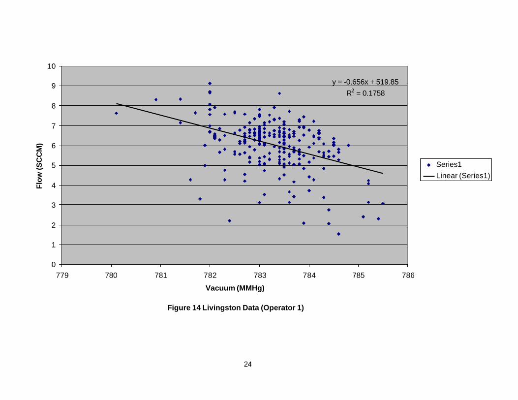
85



B1 1 0.146 -85.3 2 0.118 -25 3 0.089 -38.3 4 0.125 -56.7 5 0.198 -82.9

B2 1 0.578 -162.3 2 0.593 -78.2 3 0.105 -1 4 0.142 -17.7 5 0.146 -18.5

B3 1 0.106 -82.7 2 0.12 -33.2 3 0.083 -14.9 4 0.132 -16.9 5 0.179 -41.7

B4 1 0.223 -82.1 2 0.18 -52.7 3 0.14 -60.2 4 0.21 -67.5 5 0.138 -41.9

86



B1 1 0.071 -89.2 2 0.092 -98.4 3 0.21 -151.5 4 0.15 -124.1 5 0.092 -125.9

B2 1 0.078 -89.2 2 0.078 -77.6 3 0.112 -93.4 4 0.105 -117.6 5 0.13 -136.6

B3 1 0.142 -104.6 2 0.066 -82 3 0.134 -131.4 4 0.062 -94.1 5 0.043 -155.6

B4 1 0.153 -146.2 2 0.112 -115.1 3 0.085 -94.8 4 0.088 -99.7 5 0.115 -124.8

87



B1 1 0.257 -101.1 2 0.249 -97.7 3 0.214 -94 4 0.168 -99.6 5 0.283 -110.4

B2 1 0.229 -172 2 0.379 -107.3 3 0.285 -82.3 4 0.274 -81.9 5 0.32 -100.3

B3 1 0.314 -143.2 2 0.356 -110.2 3 0.198 -77.4 4 0.234 -69.8 5 0.195 -86.5

B4 1 0.21 -134.2 2 0.321 -114.2 3 0.708 -118.9 4 0.369 -89 5 0.623 -114.7

88



B1 1 0.146 -85.3 2 0.118 -25 3 0.089 -38.3 4 0.125 -56.7 5 0.196 -82.9

B2 1 0.578 -162.3 2 0.593 -78.2 3 0.105 -1 4 0.142 -17.7 5 0.146 -18.5

B3 1 0.106 -82.7 2 0.12 -33.2 3 0.083 -14.9 4 0.132 -16.9 5 0.179 -41.7

B4 1 0.223 -82.1 2 0.1 -52.7 3 0.14 -60.2 4 0.21 -67.5 5 0.136 -41.9

89

Table 32: Wycoff’s Bridge West Bound- cycle 1 Connection # Reading No. Corrosion Rate,


B1 1 0.061 -23.6 2 0.04 -30.4 3 0.063 -14.6 4 0.082 9.6 5 0.064 -15.1

B2 1 0.069 -40.19 2 0.059 -51.2 3 0.083 -20.9 4 0.067 7.9 5 0.089 -7.8

B3 1 0.1 -216.7 2 0.116 -30.9 3 0.059 -4.7 4 0.064 29.4 5 0.072 9.1

B4 1 0.075 -20.5 2 0.126 -23.3 3 0.068 -24 4 0.107 -65.8 5 0.066 -4.3

90



B1 1 0.15 -111.2 2 0.095 -82.3 3 0.098 -72.2 4 0.155 -92.9 5 0.11 -98.1

B2 1 0.188 -127.8 2 0.114 -95.8 3 0.104 -104.5 4 0.144 -97.6 5 0.176 -83.8

B3 1 0.121 -139 2 0.248 -120.8 3 0.204 -118.6 4 0.117 -77 5 0.15 -94.6

B4 1 0.181 -111.2 2 0.202 -101.7 3 0.079 -117.4 4 0.191 -134.8 5 0.136 -84.1

91



B1 1 0.381 -118.2 2 0.315 -110.2 3 0.4344 -118.8 4 0.119 -118.8 5 0.567 -145.1

B2 1 0.233 -202.1 2 0.233 -127.9 3 0.336 -117.2 4 0.312 -115 5 0.558 -134.9

B3 1 0.223 -163.6 2 0.303 -140.6 3 0.324 -10905 4 0.263 -108.7 5 0.468 -137.5

B4 1 0.492 -162.3 2 0.441 -141.1 3 0.277 -143.5 4 0.309 -142.9 5 0.347 -155.8

92



B1 1 0.069 -52.4 2 0.057 -49.4 3 0.066 -91.5 4 0.065 -58.7 5 0.031 -77.5

B2 1 0.037 -67.4 2 0.049 -57.8 3 0.044 -66.9 4 0.046 -76.9 5 0.059 -98.6

B3 1 0.276 -109.4 2 0.051 -65.9 3 0.096 -90.3 4 0.048 -69.7 5 0.03 -131.4

B4 1 0.021 -153.7 2 0.032 -60.3 3 0.043 -101.8 4 0.044 -66.4 5 0.042 -129.4

93



B1 1 0.15 -111.2 2 0.095 -87.3 3 0.098 -72.2 4 0.155 -92.9 5 0.11 -98.1

B2 1 0.188 -127.8 2 0.114 -95.8 3 0.104 -104.6 4 0.144 -97.6 5 0.176 -83.8

B3 1 0.121 -139 2 0.248 -120.8 3 0.204 -116.6 4 0.117 -77 5 0.15 -94.6

B4 1 0.181 -111.2 2 0.209 -101.7 3 0.079 -117.4 4 0.191 -134.8 5 0.136 -84.7

Documents

Evaluation of SHRP Equipment - Rutgers University