Embed Size (px)
Citation preview

Evaluation of Low-Cost, Centimeter-Level Accuracy OEM GNSS Receivers
Demoz Gebre-Egziabher, Principal InvestigatorDepartment of Aerospace Engineering and MechanicsUniversity of Minnesota
February 2018
Research ProjectFinal Report 2018-10
• mndot.gov/research

To request this document in an alternative format, such as braille or large print, call 651-366-4718 or 1-800-657-3774 (Greater Minnesota) or email your request to [email protected]. Please request at least one week in advance.
Technical Report Documentation Page 1. Report No. 2. 3. Recipients Accession No. MN/RC 2018-10 4. Title and Subtitle 5. Report Date Evaluation of Low-Cost, Centimeter-Level Accuracy OEM GNSS Receivers
February 2018 6.
7. Author(s) 8. Performing Organization Report No. John Jackson, Ricardo Saborio, Syed Anas Ghazanfar, Demoz Gebre-Egziabher, Brian Davis
9. Performing Organization Name and Address 10. Project/Task/Work Unit No.
Department of Aerospace Engineering and Mechanics University of Minnesota – Twin Cities 110 Union St. S.E. Minneapolis, MN 55455
CTS #2017045 11. Contract (C) or Grant (G) No.
(c) 1003325 (w) 14
12. Sponsoring Organization Name and Address 13. Type of Report and Period Covered Minnesota Department of Transportation Research Services & Library 395 John Ireland Boulevard, MS 330 St. Paul, Minnesota 55155-1899
Final Report 14. Sponsoring Agency Code
15. Supplementary Notes http:// mndot.gov/research/reports/2018/201810.pdf 16. Abstract
This report discusses the results of a study to quantify the performance of low-cost, centimeter-level accurate Global Navigation Satellite Systems (GNSS) receivers that have appeared on the market in the last few years. Centimeter-level accuracy is achieved using a complex algorithm known as real-time kinematic (RTK) processing. It involves processing correction data from a ground network of GNSS receivers in addition to the signals transmitted by the GNSS satellites. This makes RTK-capable receivers costly (in excess of $10,000) and bulky, making them unsuitable for cost- and size-sensitive transportation applications (e.g., driver assist systems in vehicles). If inexpensive GNSS receivers capable of generating a position solution with centimeter accuracy were widely available, they would push the GNSS revolution in ground transportation even further as an enabler of safety enhancements such as ubiquitous lane-departure warning systems and enhanced stability-control systems. Recently manufacturers have been advertising the availability of low-cost (< $1,000) RTK-capable receivers. The work described in this report provides an independent performance assessment of these receivers relative to high-end (and costly) receivers in realistic settings encountered in transportation applications.
17. Document Analysis/Descriptors 18. Availability Statement Satellite navigation systems, Global Positioning System, Kinematics, Geographic information systems
No restrictions. Document available from: National Technical Information Services, Alexandria, Virginia 22312
19. Security Class (this report) 20. Security Class (this page) 21. No. of Pages 22. Price Unclassified Unclassified 55

Evaluation of Low-Cost, Centimeter-Level Accuracy OEM GNSS
Receivers
FINAL REPORT
Prepared by:
John Jackson
Ricardo Saborio
Syed Anas Ghazanfar
Demoz Gebre-Egziabher
Department of Aerospace Engineering and Mechanics
University of Minnesota – Twin Cities
Brian Davis
Department of Mechanical Engineering
University of Minnesota – Twin Cities
February 2018
Published by:
Minnesota Department of Transportation
Research Services & Library
395 John Ireland Boulevard, MS 330
St. Paul, Minnesota 55155-1899
This report represents the results of research conducted by the authors and does not necessarily represent the views or policies
of the Minnesota Department of Transportation or the University of Minnesota. This report does not contain a standard or
specified technique.
The authors, the Minnesota Department of Transportation, and the University of Minnesota do not endorse products or
manufacturers. Trade or manufacturers’ names appear herein solely because they are considered essential to this report.

ACKNOWLEDGMENTS
This project was funded by and received technical support from the Minnesota Department of
Transportation. The research team would like to thank Nathan Anderson and Peter Jenkins of the Office
of Land Management’s Surveying and Mapping Section for their leadership, guidance, and feedback. The
team would also like to acknowledge all the members of the Technical Advisory Panel for their
engagement and assistance.

TABLE OF CONTENTS
CHAPTER 1: Introduction ....................................................................................................................1
CHAPTER 2: Performance Metrics .......................................................................................................3
2.1 Useful Terminology ............................................................................................................................. 3
2.2 Accuracy .............................................................................................................................................. 3
2.3 Continuity ........................................................................................................................................... 4
2.4 Availability .......................................................................................................................................... 4
2.5 Time to First Fix .................................................................................................................................. 4
CHAPTER 3: Experimental Methods ....................................................................................................5
3.1 Receiver Overview .............................................................................................................................. 5
3.2 Experimental Setup ............................................................................................................................. 6
3.3 Static Testing Methodology ................................................................................................................. 7
3.4 Dynamic Testing methodology ........................................................................................................... 9
CHAPTER 4: Experimental Results ..................................................................................................... 10
4.1 Static Testing Results ......................................................................................................................... 10
4.1.1 Accuracy .................................................................................................................................... 10
4.1.2 Continuity .................................................................................................................................. 14
4.1.3 Availability ................................................................................................................................. 18
4.1.4 Time to First RTK Solution ......................................................................................................... 20
4.2 Dynamic Testing Results .................................................................................................................... 23
4.2.1 Accuracy .................................................................................................................................... 23
4.2.2 Continuity .................................................................................................................................. 26
4.2.3 Availability ................................................................................................................................. 30
CHAPTER 5: Conclusions ................................................................................................................... 31
5.1 Discussion and Recommendations ................................................................................................... 31

5.1.1 Static Applications ..................................................................................................................... 32
5.1.2 Dynamic Applications ................................................................................................................ 33
5.2 Error Sources .................................................................................................................................... 33
5.3 Future Research ................................................................................................................................ 34
5.4 Conclusion ........................................................................................................................................ 34
REFERENCES .................................................................................................................................... 36
APPENDIX A Static Testing Tables
APPENDIX B Dynamic Testing Tables

LIST OF FIGURES
Figure 3.1 Illustration of experimental setup. .............................................................................................. 6
Figure 3.2 Experimental setup enclosed in protective container. ................................................................ 6
Figure 3.3 SCHREIBER geodetic marker north of the University of Minnesota. ........................................... 7
Figure 3.4 Rural Test Site (TURKEY MN037) ................................................................................................. 8
Figure 3.5 Suburban Test Site (UNIVERSITY1934) ......................................................................................... 8
Figure 3.6 Urban Test Site (SCHREIBER) ........................................................................................................ 9
Figure 4.1 Horizontal accuracy for RTK fixed-integer position solutions, rural location. ........................... 11
Figure 4.2 Horizontal accuracy for RTK fixed-integer position solutions, suburban location..................... 11
Figure 4.3 Horizontal accuracy for RTK fixed-integer position solutions, urban location. ......................... 12
Figure 4.4 Accuracy spread in the rural environment using the Navcom antenna. Black line indicates 5
cm. ............................................................................................................................................................... 12
Figure 4.5 Accuracy spread in the rural environment using the patch antenna. Black line indicates 5 cm
accuracy. ..................................................................................................................................................... 13
Figure 4.6 Accuracy spread in the urban environment using the Navcom antenna. Black line indicates 5
cm accuracy. ............................................................................................................................................... 13
Figure 4.7 Accuracy spread in the urban environment using the patch antenna. Black line indicates 5 cm
accuracy. ..................................................................................................................................................... 14
Figure 4.8 Horizontal accuracy for RTK floating-point position solutions, rural location. .......................... 14
Figure 4.9 Average number of times an RTK fixed-integer solution was lost per RTK minute. Black bars
indicate value of one standard deviation. Rural location. .......................................................................... 15
Figure 4.10 Average number of times an RTK fixed-integer solution was lost per RTK minute. Black bars
indicate value of one standard deviation. Suburban location. ................................................................... 16
Figure 4.11 Average number of times an RTK fixed-integer solution was lost per RTK minute. Black bars
indicate value of one standard deviation. Urban location. ........................................................................ 16
Figure 4.12 Average time to reacquire an RTK fixed-integer solution after a loss. The Eclipse P307 was
unable to reacquire an RTK fixed-integer solution after losing it with the patch antenna. Black bars
indicate value of one standard deviation. Rural location. .......................................................................... 17

Figure 4.13 Average time to reacquire an RTK fixed-integer solution after a loss. Black bars indicate value
of one standard deviation. Suburban location. .......................................................................................... 17
Figure 4.14 Average time to reacquire an RTK fixed-integer solution after a loss. Black bars indicate value
of one standard deviation. The Eclipse P307 and Piksi Multi were unable to reacquire an RTK fixed-
integer solution after losing it with the patch antenna. Urban location. ................................................... 18
Figure 4.15 Percent of time a receiver reported an RTK solution. Dark bars indicate RTK fixed-integer
solution, and light bars indicate RTK floating-point solution. Rural location. ............................................ 19
Figure 4.16 Percent of time a receiver reported an RTK solution. Dark bars indicate RTK fixed-integer
solution, and light bars indicate RTK floating-point solution. Suburban location. ..................................... 19
Figure 4.17 Percent of time a receiver reported an RTK solution. Dark bars indicate RTK fixed-integer
solution, and light bars indicate RTK floating-point solution. Urban location. ........................................... 20
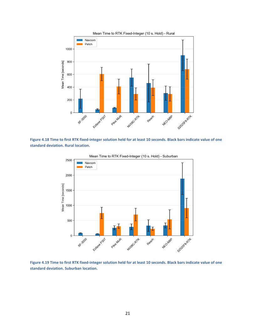
Figure 4.18 Time to first RTK fixed-integer solution held for at least 10 seconds. Black bars indicate value
of one standard deviation. Rural location. ................................................................................................. 21
Figure 4.19 Time to first RTK fixed-integer solution held for at least 10 seconds. Black bars indicate value
of one standard deviation. Suburban location. .......................................................................................... 21
Figure 4.20 Time to first RTK fixed-integer solution held for at least 10 seconds. Black bars indicate value
of one standard deviation. Urban location. ................................................................................................ 22
Figure 4.21 Time to first RTK floating-point solution. Black bars indicate value of one standard deviation.
Urban location. ........................................................................................................................................... 22
Figure 4.22 Horizontal accuracy for dynamic RTK fixed-integer position solutions. .................................. 24
Figure 4.23 Fixed-integer dynamic accuracy spread in the rural environment. Black line indicates 5 cm
accuracy. ..................................................................................................................................................... 24
Figure 4.24 Fixed-integer dynamic accuracy spread in the urban environment. Black line indicates 5 cm
accuracy. ..................................................................................................................................................... 25
Figure 4.25 Floating-point dynamic accuracy spread in the rural environment. ....................................... 25
Figure 4.26 Mean Number of RTK Fixed-Integer Lock Losses ..................................................................... 26
Figure 4.27 Mean Time to RTK Fixed-Integer Reacquisition ....................................................................... 27
Figure 4.28 RTK losses and reacquisitions on the southbound bridges route. ........................................... 28
Figure 4.29 RTK losses and reacquisitions on the northbound bridges route. ........................................... 29
Figure 4.30 Mean Time in RTK Fixed-Integer Solution................................................................................ 30
LIST OF TABLES
Table 3.1 Summary of receivers used for testing. ........................................................................................ 5
Table 3.2 Geodetic markers used for static tests. ........................................................................................ 7
Table 3.3 Dynamic testing route descriptions. ............................................................................................. 9
Table 5.1 Best-case statistics for each receiver from static testing in the rural environment. .................. 32
Table 5.2 Statistics for each receiver from dynamic testing on the rural route. ........................................ 33
Table A.1 Horizontal accuracy for RTK fixed-integer positions. ................................................................ A-1
Table A.2 Horizontal accuracy for RTK floating-point positions. .............................................................. A-1
Table A.3 Mean number of RTK fix losses per RTK minute. ...................................................................... A-1
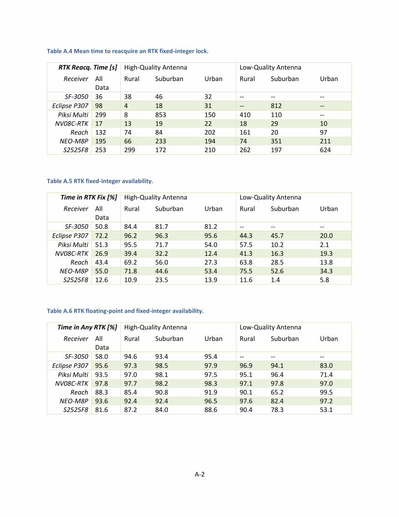
Table A.4 Mean time to reacquire an RTK fixed-integer lock. .................................................................. A-2
Table A.5 RTK fixed-integer availability. ................................................................................................... A-2
Table A.6 RTK floating-point and fixed-integer availability. ..................................................................... A-2
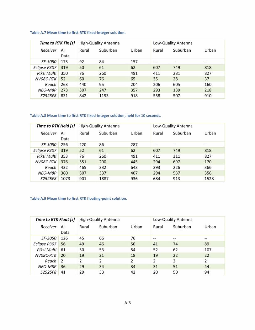
Table A.7 Mean time to first RTK fixed-integer solution. ......................................................................... A-3
Table A.8 Mean time to first RTK fixed-integer solution, held for 10 seconds. ........................................ A-3
Table A.9 Mean time to first RTK floating-point solution. ........................................................................ A-3
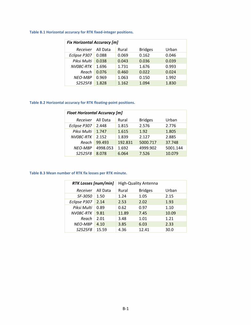
Table B.1 Horizontal accuracy for RTK fixed-integer positions. ................................................................. B-1
Table B.2 Horizontal accuracy for RTK floating-point positions. ............................................................... B-1
Table B.3 Mean number of RTK fix losses per RTK minute. ....................................................................... B-1
Table B.4 Mean time to reacquire an RTK fixed-integer lock. ................................................................... B-2
Table B.5 RTK fixed-integer availability...................................................................................................... B-2
Table B.6 RTK floating-point and fixed-integer availability. ....................................................................... B-2
EXECUTIVE SUMMARY
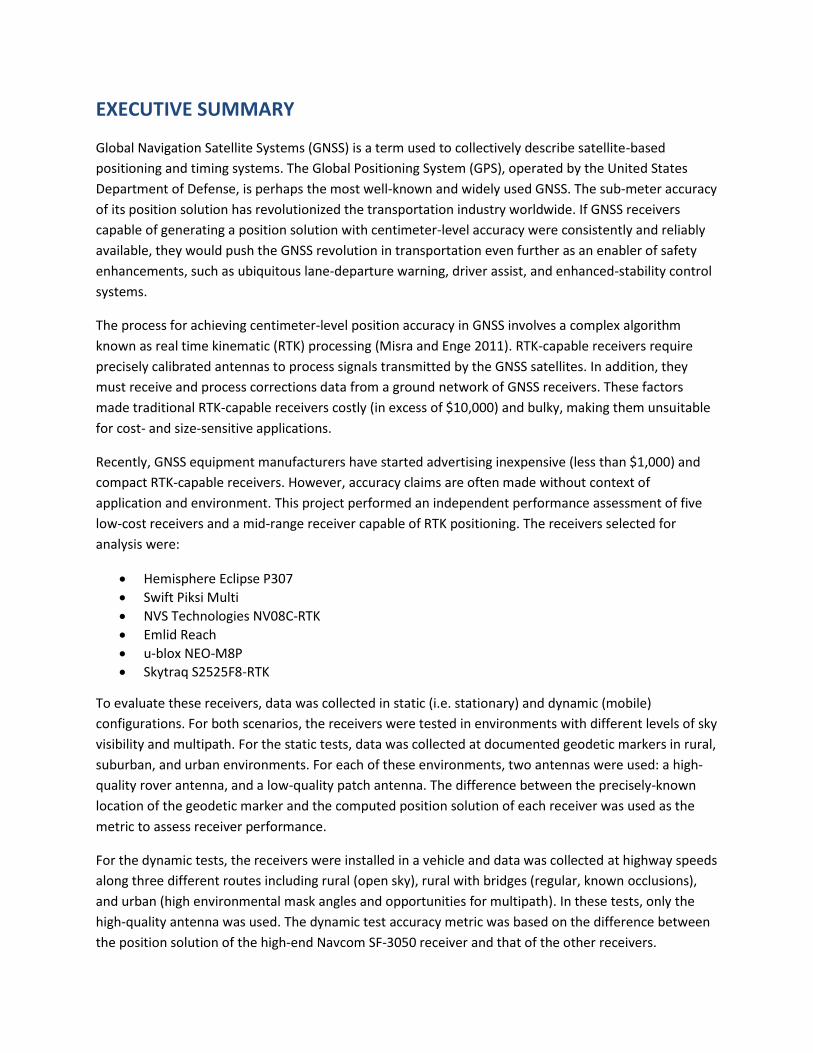
Global Navigation Satellite Systems (GNSS) is a term used to collectively describe satellite-based
positioning and timing systems. The Global Positioning System (GPS), operated by the United States
Department of Defense, is perhaps the most well-known and widely used GNSS. The sub-meter accuracy
of its position solution has revolutionized the transportation industry worldwide. If GNSS receivers
capable of generating a position solution with centimeter-level accuracy were consistently and reliably
available, they would push the GNSS revolution in transportation even further as an enabler of safety
enhancements, such as ubiquitous lane-departure warning, driver assist, and enhanced-stability control
systems.
The process for achieving centimeter-level position accuracy in GNSS involves a complex algorithm
known as real time kinematic (RTK) processing (Misra and Enge 2011). RTK-capable receivers require
precisely calibrated antennas to process signals transmitted by the GNSS satellites. In addition, they
must receive and process corrections data from a ground network of GNSS receivers. These factors
made traditional RTK-capable receivers costly (in excess of $10,000) and bulky, making them unsuitable
for cost- and size-sensitive applications.
Recently, GNSS equipment manufacturers have started advertising inexpensive (less than $1,000) and
compact RTK-capable receivers. However, accuracy claims are often made without context of
application and environment. This project performed an independent performance assessment of five
low-cost receivers and a mid-range receiver capable of RTK positioning. The receivers selected for
analysis were:
Hemisphere Eclipse P307
Swift Piksi Multi
NVS Technologies NV08C-RTK
Emlid Reach
u-blox NEO-M8P
Skytraq S2525F8-RTK
To evaluate these receivers, data was collected in static (i.e. stationary) and dynamic (mobile)
configurations. For both scenarios, the receivers were tested in environments with different levels of sky
visibility and multipath. For the static tests, data was collected at documented geodetic markers in rural,
suburban, and urban environments. For each of these environments, two antennas were used: a high-
quality rover antenna, and a low-quality patch antenna. The difference between the precisely-known
location of the geodetic marker and the computed position solution of each receiver was used as the
metric to assess receiver performance.
For the dynamic tests, the receivers were installed in a vehicle and data was collected at highway speeds
along three different routes including rural (open sky), rural with bridges (regular, known occlusions),
and urban (high environmental mask angles and opportunities for multipath). In these tests, only the
high-quality antenna was used. The dynamic test accuracy metric was based on the difference between
the position solution of the high-end Navcom SF-3050 receiver and that of the other receivers.

The static tests showed that the low-cost receivers have 10 cm (95%) or better RTK fixed-integer
horizontal accuracy in the rural, low-multipath environment using the high-quality antenna. In the
suburban and urban environments with moderate to high multipath, low-cost receiver accuracies
degraded to over 1 meter in some cases. The RTK fixed-integer availability ranged from 1.4% to 75.5%
using the low-cost antenna, and 10.9% to 95.5% using the high-quality antenna. However, all low-cost
receivers had a minimum RTK floating-point or fixed integer availability of 84% and 53.1% using the
high-quality and low-quality antenna, respectively. This suggests that the high-quality antenna is
favorable for RTK availability.
The results of the dynamic tests suggest that the single frequency receivers are not well suited for
dynamic applications. The best single-frequency RTK fixed-integer availability was 25.5%. The
multifrequency receivers had RTK fixed-integer availabilities with values ranging from 29.6% to 57.4%.
The RTK fixed-integer integer horizontal position accuracies of the low-cost receivers with respect to the
SF-3050 range from 1.5 cm to 1.8 m (95%). The RTK floating-point horizontal position accuracies ranged
from 1.7 m to 10 m in general, though spurious behavior was observed, which had extreme accuracy
values up to 5 km (95%). The bridges route revealed that only two receivers being tested – the Piksi
Multi and Eclipse P307 – had an RTK fixed-integer solution consistent enough to warrant RTK fix loss
study. The Piksi Multi took twice as long as the Eclipse P307 and more than four times longer than the
SF-3050 to reacquire an RTK fixed-integer solution after passing under a bridge.
The cumulative results suggest that L1-only RTK receivers face challenges related to positioning
robustness and continuity when applied in more varied environments. However, they have potential in
applications that have low-dynamics and open skies. The Piksi Multi receiver showed better
performance in continuity in the dynamic scenarios and is recommended for future study for on-vehicle
applications. However, it is still susceptible to degraded accuracy in more obstructed and multipath-
prone environments.
Considering it is not a low-cost receiver, the Eclipse P307 performed well in static and dynamic tests in
all environments. It was versatile in that it used both the low-quality and high-quality antennas for RTK
positioning, while the reference receiver could not. However, its cost is an order of magnitude higher
than the low-cost receivers.
The results in this report give an idea of the accuracy and continuity of low-cost GNSS receivers relative
to established reference receivers. Future studies could examine the effects of future firmware releases
on receiver performance, a focused study on better-performing low-cost receivers, or application-
specific experiments.

1
CHAPTER 1: INTRODUCTION
Global Navigation Satellite Systems (GNSS) is a term used to collectively describe satellite-based
positioning and timing systems. The Global Positioning System (GPS), operated by the United States
Department of Defense, is perhaps the most well-known and widely used GNSS. The sub-meter accuracy
of its position solution has revolutionized road, rail, air, and marine transportation systems worldwide.
Its timing function is the de-facto heartbeat for clocks around the globe in support of operations such as
time stamping of banking transactions and synchronizing electrical frequency on interconnected power
grids (GPS.gov 2014).
In general, GPS can deliver a position solution with accuracy on the order of several meters. Sub-meter
accuracy can be achieved but requires additional processing and external data. For example, centimeter-
level accuracy in GNSS is achieved using a complex algorithm known as real-time kinematic (RTK)
processing (Misra and Enge 2011). RTK-capable receivers require precisely calibrated antennas that
process signals transmitted by the GNSS satellites. In addition, they must receive and process
corrections data from a ground network of GNSS receivers. This makes RTK-capable receivers costly (in
excess of $10,000) and bulky, making them unsuitable for cost- and size-sensitive automotive
applications. If inexpensive GNSS receivers capable of generating a position solution with centimeter-
level accuracy were widely available, they would push the GNSS revolution in ground transportation
even further as an enabler of safety enhancements such as ubiquitous lane-departure warnings systems,
driver assist systems, and enhanced stability control systems.
Recently, GNSS equipment manufacturers have started advertising inexpensive (less than $1,000) and
compact RTK-capable receivers. However, data supporting these accuracy claims is not publicly
available. The work performed in this project aims to provide an independent performance assessment
of six low-cost, RTK-capable receivers. The motivation was to determine the performance of these
receivers in a number of realistic scenarios to assess their suitability for intelligent transportation
applications. More precisely, the project goal was to answer the following question: Are the new,
purportedly RTK-capable, inexpensive receivers able to perform at the same level as high-end, survey-
grade receivers such as the Navcom SF-3050, Novatel OEM7700 or Trimble BX982?
A major benefit of and motivation for the work is to aid in the development and evolution of the
Minnesota Continuously Operating Reference Station (MnCORS) network. Generating an RTK solution
requires processing GNSS satellite signals alongside the information received from a network of
stationary base stations. In Minnesota, the primary users of the MnCORS network are land and
construction surveyors. If the new RTK-capable receivers can provide centimeter-level accuracy
inexpensively, it may lead to a surge in the user base demanding access to the MnCORS network. In
order to better understand and predict demand, the MnCORS operators were interested in an

2
evaluation of currently available technology. Interest was in low-cost hardware, which if reliable
enough, would be more likely to see rapid adoption.
This report documents the work performed to answer the above question. Chapter 2 introduces the
performance metrics used for this study. Chapter 3 describes the experiments performed to collect the
receiver evaluation data including the hardware used and the experimental methods used to collect the
data. Chapter 4 summarizes the results of the static and dynamic testing performed on the receivers.
Chapter 5 discusses the implications of the receivers’ performance noted in this study and offers
suggestions for future evaluations.
3
CHAPTER 2: PERFORMANCE METRICS
This chapter describes the metrics used to compare the receivers to one another. The following four
metrics were used: Accuracy, Continuity, Availability, and Time to First Fix. These are loosely based off
metrics defined in the GPS Standard Positioning Solution Performance Standard (U.S Department of
Defense, 2008).
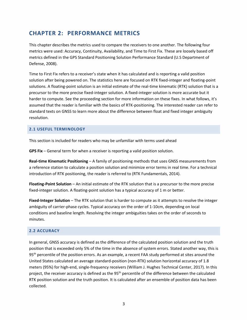
Time to First Fix refers to a receiver’s state when it has calculated and is reporting a valid position
solution after being powered on. The statistics here are focused on RTK fixed-integer and floating-point
solutions. A floating-point solution is an initial estimate of the real-time kinematic (RTK) solution that is a
precursor to the more precise fixed-integer solution. A fixed-integer solution is more accurate but it
harder to compute. See the proceeding section for more information on these fixes. In what follows, it’s
assumed that the reader is familiar with the basics of RTK-positioning. The interested reader can refer to
standard texts on GNSS to learn more about the difference between float and fixed integer ambiguity
resolution.
2.1 USEFUL TERMINOLOGY
This section is included for readers who may be unfamiliar with terms used ahead
GPS Fix – General term for when a receiver is reporting a valid position solution.
Real-time Kinematic Positioning – A family of positioning methods that uses GNSS measurements from
a reference station to calculate a position solution and minimize error terms in real time. For a technical
introduction of RTK positioning, the reader is referred to (RTK Fundamentals, 2014).
Floating-Point Solution – An initial estimate of the RTK solution that is a precursor to the more precise
fixed-integer solution. A floating-point solution has a typical accuracy of 1 m or better.
Fixed-Integer Solution – The RTK solution that is harder to compute as it attempts to resolve the integer
ambiguity of carrier-phase cycles. Typical accuracy on the order of 1-10cm, depending on local
conditions and baseline length. Resolving the integer ambiguities takes on the order of seconds to
minutes.
2.2 ACCURACY
In general, GNSS accuracy is defined as the difference of the calculated position solution and the truth
position that is exceeded only 5% of the time in the absence of system errors. Stated another way, this is
95th percentile of the position errors. As an example, a recent FAA study performed at sites around the
United States calculated an average standard-position (non-RTK) solution horizontal accuracy of 1.8
meters (95%) for high-end, single-frequency receivers (William J. Hughes Technical Center, 2017). In this
project, the receiver accuracy is defined as the 95th percentile of the difference between the calculated
RTK position solution and the truth position. It is calculated after an ensemble of position data has been
collected.

4
2.3 CONTINUITY
The formal definition of continuity is the likelihood of a detected but unscheduled navigation function
interruption after an operation has been initiated. As shown later, the RTK solution is not always
available. Once a receiver has computed an RTK fixed-integer solution, there are situations that may
cause the receiver to lose the fixed-integer solution and revert to a floating-point solution. This loss of
RTK lock is a loss of continuity. The work here used two additional metrics to characterize continuity:
Loss of Lock Frequency – The number of loss of RTK fixed-integer locks per RTK minute
Average Time to Reacquire – The average time to reacquire the RTK fixed-integer solution after
it is lost
The loss of lock frequency is normalized by the amount of time a receiver spent in RTK fixed-integer
mode. This was done to make comparisons between receivers that have different RTK availability values.
2.4 AVAILABILITY
The definition of availability used here is not the same as the standard definition of the term used in the
navigation community. The RTK availability is defined as the total amount of time as a percentage that a
receiver spends in an RTK position solution. An ideal receiver will have an RTK availability close to 100%.
RTK availability statistics are reported in two ways:
RTK Fixed-Integer Availability – Total percentage of experimental time spent in a fixed-integer
solution
RTK Floating-Point and Fixed-Integer Availability – Total percentage of experimental time spent
in a fixed-integer and floating-point solution
2.5 TIME TO FIRST FIX
The time to fist fix (TTFF) is a performance metric of receiver initialization. It is the amount of time that it
takes to report a solution from a cold start (no knowledge left over from its previous operational state).
A hold-condition of 10 seconds was imposed on the RTK fixed-integer solution. Two TTFF metrics are
considered here:
TTFF RTK Floating-Point - Time to compute the initial floating-point solution
TTFF RTK Fixed-Integer - Time to compute the initial fixed-integer solution and subsequently
hold the solution for 10 seconds
The requirement of holding the TTFF RTK fixed-integer position for 10 seconds was imposed because it
was common for receivers to report a fixed-integer solution initially, then then report it lost the next
timestep.
5
CHAPTER 3: EXPERIMENTAL METHODS
3.1 RECEIVER OVERVIEW
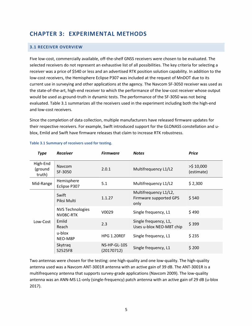
Five low-cost, commercially available, off-the-shelf GNSS receivers were chosen to be evaluated. The
selected receivers do not represent an exhaustive list of all possibilities. The key criteria for selecting a
receiver was a price of $540 or less and an advertised RTK position solution capability. In addition to the
low-cost receivers, the Hemisphere Eclipse P307 was included at the request of MnDOT due to its
current use in surveying and other applications at the agency. The Navcom SF-3050 receiver was used as
the state-of-the-art, high-end receiver to which the performance of the low-cost receiver whose output
would be used as ground-truth in dynamic tests. The performance of the SF-3050 was not being
evaluated. Table 3.1 summarizes all the receivers used in the experiment including both the high-end
and low-cost receivers.
Since the completion of data collection, multiple manufacturers have released firmware updates for
their respective receivers. For example, Swift introduced support for the GLONASS constellation and u-
blox, Emlid and Swift have firmware releases that claim to increase RTK robustness.
Table 3.1 Summary of receivers used for testing.
Type Receiver Firmware Notes Price
High-End (ground truth)
Navcom SF-3050
2.0.1 Multifrequency L1/L2 >$ 10,000 (estimate)
Mid-Range Hemisphere Eclipse P307
5.1 Multifrequency L1/L2 $ 2,300
Low-Cost
Swift Piksi Multi
1.1.27 Multifrequency L1/L2, Firmware supported GPS only
$ 540
NVS Technologies NV08C-RTK
V0029 Single frequency, L1 $ 490
Emlid Reach
2.3 Single frequency, L1, Uses u-blox NEO-M8T chip
$ 399
u-blox NEO-M8P
HPG 1.20REF Single frequency, L1 $ 235
Skytraq S2525F8
NS-HP-GL-10S (20170712)
Single frequency, L1 $ 200
Two antennas were chosen for the testing: one high-quality and one low-quality. The high-quality
antenna used was a Navcom ANT-3001R antenna with an active gain of 39 dB. The ANT-3001R is a
multifrequency antenna that supports survey-grade applications (Navcom 2009). The low-quality
antenna was an ANN-MS L1-only (single-frequency) patch antenna with an active gain of 29 dB (u-blox
2017).

6
3.2 EXPERIMENTAL SETUP
The receivers were connected to a single antenna through a GPS Technologies ALDCV1x8 signal splitter.
They were connected to the laptop computer via USB that ran the data collection software. The data
collection software is a custom application built in Python. RTK corrections data was provided by the
Minnesota Continually Operating Reference Station (MnCORS) Network (MnDOT, 2018a). This service
was accessed over the internet by connecting the laptop to a cellular modem. Error! Reference source
not found. shows a diagram of the experimental setup and Error! Reference source not found. shows a
diagram of the experimental setup and Error! Reference source not found.Error! Reference source not
found. shows the experimental setup with low-cost receivers enclosed in a protective container.
Figure 3.1 Illustration of experimental setup.
Figure 3.2 Experimental setup enclosed in protective container.
The receiver output was in the form on National Marine Electronics Association (NMEA) strings, a
common ASCII format used for reporting calculated positioning products. The GGA string contains the

7
latitude, longitude, position-fix type and other relevant information about the GPS fix of the receiver. An
example NMEA string is:
$GNGGA,205450.00,4458.86243,N,09314.77762,W,4,12,0.70,250.8,M,-30.9,M,2.0,0527*59
Which contains latitude, longitude, GPS fix status, number of satellites and other information. For more
information regarding the NMEA standard, refer to the NMEA 0183 V 4.10 standards document.
3.3 STATIC TESTING METHODOLOGY
Static testing was conducted in three different environments using test points found using MnDOT’s
interactive geodetic monument viewer (MnDOT, 2018b). An example of a survey marker used is shown
in Figure 3.3. The three environments were chosen to best reflect the qualitative characteristics of rural,
suburban and urban settings. Rural areas have a clear view of the sky with no obstructions or nearby
metal structures. Urban areas have tall, metal structures and a narrower view of the sky from the
antenna’s point-of-view. Suburban areas fall somewhere in-between. The chosen markers were a
compromise in the availability of markers and desired environmental features.
Table 3.2 Geodetic markers used for static tests.
Environment Marker ID Horizontal Accuracy Vertical Accuracy
Urban SCHREIBER 2.13 mm 4.88 mm
Suburban UNIVERSITY1934 1.01 cm 2.13 mm
Rural TURKEY MN037 4.88 mm 4.88 mm
Static data was collected in 25-minute-long sessions on 17 days over 4 months. Each antenna-
environment combination was repeated a minimum of 6 times to establish significance in the TTFF
statistics.
Figure 3.3 SCHREIBER geodetic marker north of the University of Minnesota.

8
Figure 3.4 Rural Test Site (TURKEY MN037)
Figure 3.5 Suburban Test Site (UNIVERSITY1934)
9
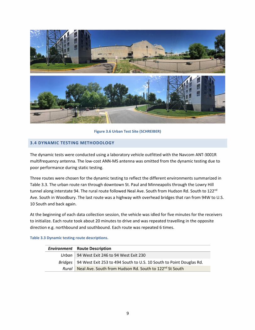
Figure 3.6 Urban Test Site (SCHREIBER)
3.4 DYNAMIC TESTING METHODOLOGY
The dynamic tests were conducted using a laboratory vehicle outfitted with the Navcom ANT-3001R
multifrequency antenna. The low-cost ANN-MS antenna was omitted from the dynamic testing due to
poor performance during static testing.
Three routes were chosen for the dynamic testing to reflect the different environments summarized in
Table 3.3. The urban route ran through downtown St. Paul and Minneapolis through the Lowry Hill
tunnel along interstate 94. The rural route followed Neal Ave. South from Hudson Rd. South to 122nd
Ave. South in Woodbury. The last route was a highway with overhead bridges that ran from 94W to U.S.
10 South and back again.
At the beginning of each data collection session, the vehicle was idled for five minutes for the receivers
to initialize. Each route took about 20 minutes to drive and was repeated travelling in the opposite
direction e.g. northbound and southbound. Each route was repeated 6 times.
Table 3.3 Dynamic testing route descriptions.
Environment Route Description
Urban 94 West Exit 246 to 94 West Exit 230
Bridges 94 West Exit 253 to 494 South to U.S. 10 South to Point Douglas Rd.
Rural Neal Ave. South from Hudson Rd. South to 122nd St South
10
CHAPTER 4: EXPERIMENTAL RESULTS
4.1 STATIC TESTING RESULTS
In this section the results of the static tests are presented. Recall that for the static tests the position
error that was used to calculate the accuracy metric came from taking the difference between the
respective receivers’ position solution and the known position of the survey monument where the
antennas were located. The values used to populate each figure are found in Appendix A.
4.1.1 Accuracy
Figure 4.1, Figure 4.2 and Figure 4.3 illustrate the horizontal accuracy of each receiver in each
environment. In the figures that follow, each bar color represents an antenna type (left to right): blue
for the Navcom ANT3001R and orange for the u-blox ANN-MS Patch antenna. The SF-3050 (the ground-
truth source for the dynamic tests) requires a specifically designed, multifrequency antenna to operate.
As such, for the SF-3050 the only results shown are those using the high-end antenna and are for
comparison purposes only.
The most pertinent results are those taken in the rural environment and shown in Figure 4.1 as this can
be considered the best-case scenario. Examination of the results indicates that the Eclipse P307 and the
NEO-MP8 have performance that is close to the SF-3050 using either antenna.
To get a better picture of RTK fixed-integer errors in the rural environment, an accuracy spread is shown
in Figure 4.4 and Error! Reference source not found. for the high-quality and patch antennas,
respectively. Some receivers exhibit a steep accuracy degradation as its threshold approaches 95%. For
the high-end antenna, the Reach and S2525F8-RTK exhibit the degradation around the 75th percentile.
For the NEO-M8P and NV08C-RTK, the degradation occurs above the 90th percentile when their spikes
occur. For the patch antenna, the NV08C-RTK has poor accuracy from the 50th percentile, while the Piksi
Multi degrades after the 70th percentile. This means that the error distribution from these receivers is
heavy-tailed relative to a Gaussian distribution. It highlights the fact that receiver manufacturers report
their RTK fixed-integer accuracies using different methodologies, such as Circular Error Probability (50th
percentile) or 1σ (~68th percentile).
As expected, the suburban and urban environments had a negative impact on the RTK fixed-integer
accuracy of the low-cost receivers. Observation of Figure 4.2 and Figure 4.3 show no clear relationship
between accuracy in antenna quality. These are environments replete with multipath sources that
introduce error into the measured signals, as expected. These challenges are minimized in the open-sky,
rural environment. Methods exist for multipath detection and mitigation (Braasch 1995) and are
employed by some receivers such as the Eclipse P307, which maintained centimeter-level accuracies
across all testing environments. The effects are evident in Figure 4.6 and Figure 4.10, which show the
accuracy spread in the urban environment. Using the high-end antenna, most receivers maintain 5 cm
accuracy up to the 60th percentile until errors become more pronounced. Using the patch antenna, most
receivers have accuracy values worse than 10 cm at the 50th percentile.

11
Figure 4.8 illustrates the RTK floating-point solution accuracies in the rural environment. While less
accurate than the RTK fixed-integer solution, a receiver will return to the floating-point solution if it
loses its fixed-integer lock. What is apparent from this figure is that there is no clear relationship
between antenna quality and the accuracy of the RTK floating-point solution.
Figure 4.1 Horizontal accuracy for RTK fixed-integer position solutions, rural location.
Figure 4.2 Horizontal accuracy for RTK fixed-integer position solutions, suburban location.

12
Figure 4.3 Horizontal accuracy for RTK fixed-integer position solutions, urban location.
Figure 4.4 Accuracy spread in the rural environment using the Navcom antenna. Black line indicates 5 cm.

13
Figure 4.5 Accuracy spread in the rural environment using the patch antenna. Black line indicates 5 cm accuracy.
Figure 4.6 Accuracy spread in the urban environment using the Navcom antenna. Black line indicates 5 cm
accuracy.

14
Figure 4.7 Accuracy spread in the urban environment using the patch antenna. Black line indicates 5 cm
accuracy.
Figure 4.8 Horizontal accuracy for RTK floating-point position solutions, rural location.
4.1.2 Continuity
As noted in Chapter 2, continuity performance was assessed as two metrics. First, the frequency of loss-
of-lock was assessed. This metric was computed by observing how often the receivers self-reported a

15
loss of lock over a minute of RTK fixed-integer operation. The receivers’ performance in each
environment relative to this metric are shown in Figure 4.9, Figure 4.10 and Figure 4.11. Except for the
NV08C-RTK and S2525F8-RTK, there was a correlation between environment and the average number of
losses where in a rural environment it is less likely to lose an RTK lock. Except for the NV08C-RTK and
S2525F8-RTK again, using the high-quality antenna was less likely to result in a loss of lock. The S2525F8-
RTK and NV08C-RTK were prone to RTK fixed-integer lock losses in all environments.
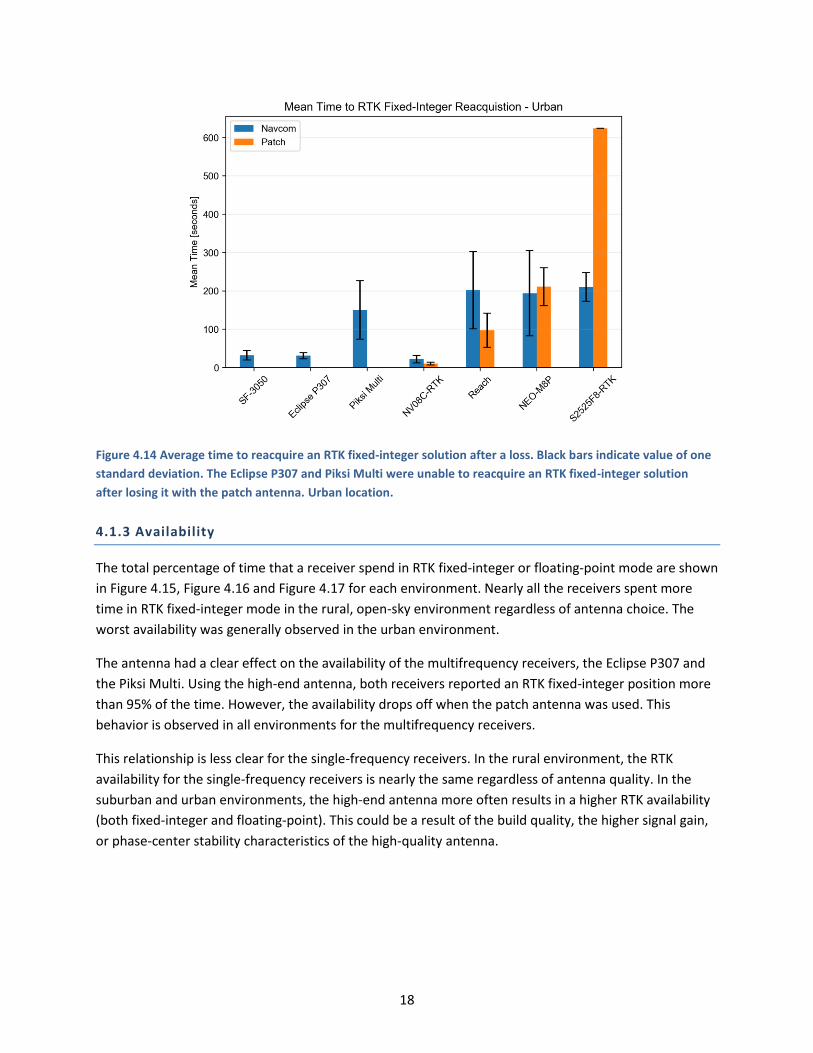
The second metric is the average time taken by the receiver to reacquire the RTK fixed-integer solution
shown in Figure 4.12, Figure 4.13 and Figure 4.14 for each environment. Using the patch antenna
resulted in cases where RTK fixed-integer reacquisition did not take place within the experimental time,
such as the Eclipse P307 in the rural and urban environments. This isn’t to say it would not reacquire the
RTK fixed-integer solution ever, but that it may have taken longer than the data run to do so. In the rural
environment, the high-quality antenna usually led to quicker RTK reacquisition times. In the other
environments, there is no clear relationship between antenna quality and the RTK reacquisition time.
Curiously, the Piksi Multi reported a reacquisition time greater than 800 seconds in the suburban
environment using the high-quality antenna.
The reacquisition times reported here are generally well below the RTK fixed-integer initialization times
reported later, as the requirement for this statistic was defined less stringent than the RTK initialization
time. However, care should be taken in interpreting these results. Since it is not known what the criteria
each receiver uses for defining the quality of their RTK locks, it is difficult to say that the absolute
performance of one receiver is better than the other.
Figure 4.9 Average number of times an RTK fixed-integer solution was lost per RTK minute. Black bars indicate
value of one standard deviation. Rural location.

16
Figure 4.10 Average number of times an RTK fixed-integer solution was lost per RTK minute. Black bars indicate
value of one standard deviation. Suburban location.
Figure 4.11 Average number of times an RTK fixed-integer solution was lost per RTK minute. Black bars indicate
value of one standard deviation. Urban location.

17
Figure 4.12 Average time to reacquire an RTK fixed-integer solution after a loss. The Eclipse P307 was unable to
reacquire an RTK fixed-integer solution after losing it with the patch antenna. Black bars indicate value of one
standard deviation. Rural location.
Figure 4.13 Average time to reacquire an RTK fixed-integer solution after a loss. Black bars indicate value of one
standard deviation. Suburban location.
18
Figure 4.14 Average time to reacquire an RTK fixed-integer solution after a loss. Black bars indicate value of one
standard deviation. The Eclipse P307 and Piksi Multi were unable to reacquire an RTK fixed-integer solution
after losing it with the patch antenna. Urban location.
4.1.3 Availability
The total percentage of time that a receiver spend in RTK fixed-integer or floating-point mode are shown
in Figure 4.15, Figure 4.16 and Figure 4.17 for each environment. Nearly all the receivers spent more
time in RTK fixed-integer mode in the rural, open-sky environment regardless of antenna choice. The
worst availability was generally observed in the urban environment.
The antenna had a clear effect on the availability of the multifrequency receivers, the Eclipse P307 and
the Piksi Multi. Using the high-end antenna, both receivers reported an RTK fixed-integer position more
than 95% of the time. However, the availability drops off when the patch antenna was used. This
behavior is observed in all environments for the multifrequency receivers.
This relationship is less clear for the single-frequency receivers. In the rural environment, the RTK
availability for the single-frequency receivers is nearly the same regardless of antenna quality. In the
suburban and urban environments, the high-end antenna more often results in a higher RTK availability
(both fixed-integer and floating-point). This could be a result of the build quality, the higher signal gain,
or phase-center stability characteristics of the high-quality antenna.

19
Figure 4.15 Percent of time a receiver reported an RTK solution. Dark bars indicate RTK fixed-integer solution,
and light bars indicate RTK floating-point solution. Rural location.
Figure 4.16 Percent of time a receiver reported an RTK solution. Dark bars indicate RTK fixed-integer solution,
and light bars indicate RTK floating-point solution. Suburban location.

20
Figure 4.17 Percent of time a receiver reported an RTK solution. Dark bars indicate RTK fixed-integer solution,
and light bars indicate RTK floating-point solution. Urban location.
4.1.4 Time to First RTK Solution
The average time to first RTK fixed-integer solution held for 10 seconds are shown in Figure 4.18, Figure
4.19 and Figure 4.20 for each environment. The time to acquire an RTK solution is dependent on the
quality of the received GNSS signals (which is affected by propagation errors as well as antenna phase
center motion) and the algorithm built into its firmware. Calculating an RTK floating-point solution is
relatively simple once a receiver computes its initial position solution and begins to receive corrections
data from MnCORS. Thus, the focus is on the fixed-integer solution performance only.
Examining the RTK initialization in the rural environment in Figure 4.18, there is a clear benefit to using
the high-quality, multifrequency antenna with the multifrequency receivers. By using two or more
frequencies, a receiver essentially has double or more information at hand which will make RTK
initialization quicker. This benefit is lost when using the single-frequency patch antenna. Observing the
single-frequencies suggest that the initialization process is slightly worsened with the high-quality antenna
though the initialization times are nearly the same for the NEO-M8P.
RTK floating-point initialization for the rural environment is presented in Figure 4.21. All receivers had an
initialization time under one minute with no dependence on antenna quality. Rather, a receiver would
calculate its initial RTK floating-point solution as soon as it had its first valid 3D position fix and MnCORS
correction data available. RTK floating-point initialization times did not vary greatly between testing
environments.
21
Figure 4.18 Time to first RTK fixed-integer solution held for at least 10 seconds. Black bars indicate value of one
standard deviation. Rural location.
Figure 4.19 Time to first RTK fixed-integer solution held for at least 10 seconds. Black bars indicate value of one
standard deviation. Suburban location.

22
Figure 4.20 Time to first RTK fixed-integer solution held for at least 10 seconds. Black bars indicate value of one
standard deviation. Urban location.
Figure 4.21 Time to first RTK floating-point solution. Black bars indicate value of one standard deviation. Urban
location.

23
4.2 DYNAMIC TESTING RESULTS
The dynamic test metrics are broken down in the same manner as the static test metrics. Time to first
RTK solutions have been omitted as they don’t contribute to the analysis of the dynamic test cases. The
values used to populate each figure are found in Appendix B.
4.2.1 Accuracy
The calculated position output of the Navcom SF-3050 receiver was used as the truth position to calculate
the low-cost receiver accuracies. The horizontal accuracies of the fixed-integer solutions are shown in
Error! Reference source not found.. In the figures that follow each bar color represents a different
location (left to right): red for the rural route, brown for the bridges route, and purple for the urban route.
The multifrequency receivers maintained an accuracy of 16 cm or better on all routes, whereas the others
did not. The Reach maintained accuracies of 2 cm on the suburban and urban routes and NEO-M8P had
an accuracy of 15 cm on the bridges route, but worse accuracies on the other routes.
To resolve the poor accuracy characteristics in dynamic testing, a range of accuracies was illustrated.
Many receiver manufacturers report 50% or 1σ (~68%) accuracy rather than 95% accuracy. Accuracy
spread plots that range from the 50th to 95th percentile are shown in Figure 4.23 and Figure 4.24 for the
rural and urban environments. At the 50th and 68th percentiles, accuracies for most receivers is still 10 cm
or better. However, once the 90th percentile is reached, many receivers accuracies diverge towards 1+
meters.
The accuracy of the RTK floating-point solutions was within expected ranges, save for the Reach and NEO-
M8P. An accuracy spread plot is shown in Figure 4.25. Whereas most receivers maintain floating-point
accuracies on the order of 1 meter, anomalies occurred with the Reach and NEO-M8P that resulted in
divergent position solutions. The worst of these divergent errors was on the order of 1 kilometer.

24
Figure 4.22 Horizontal accuracy for dynamic RTK fixed-integer position solutions.
Figure 4.23 Fixed-integer dynamic accuracy spread in the rural environment. Black line indicates 5 cm accuracy.

25
Figure 4.24 Fixed-integer dynamic accuracy spread in the urban environment. Black line indicates 5 cm accuracy.
Figure 4.25 Floating-point dynamic accuracy spread in the rural environment.

26
4.2.2 Continuity
The dynamic route with bridges was chosen specifically to explore the explicit RTK fixed-integer loss of
lock frequency and reacquisition time when travelling under bridges. The only receivers that had an RTK
fixed-integer lock consistent enough to evaluate the effects of bridges were the Piksi Multi and Eclipse
P307. Error! Reference source not found. contains information about the mean number of RTK fix
losses. These three receivers have the same mean loss of RTK instances in the bridges route.
There was no distinction made in the data between a loss of RTK due to bridges or a different cause e.g.
a hauling truck or a retaining wall. However, Figure 4.28 and Figure 4.29 show a portion of the bridge
route with colors corresponding to RTK-position fix type. The Eclipse P307 fell into an RTK floating-point
solution almost immediately, then reacquired the RTK fixed-integer solution 19 seconds later. The Piksi
Multi completely lost its RTK solution after travelling under a bridge and takes about 41 seconds to
reacquire an RTK fixed-integer solution. The SF-3050 reacquired its RTK lock in 7 seconds.
Figure 4.26 Mean Number of RTK Fixed-Integer Lock Losses

27
Figure 4.27 Mean Time to RTK Fixed-Integer Reacquisition

28
Figure 4.28 RTK losses and reacquisitions on the southbound bridges route.
A: Piksi Multi
B: Eclipse P307
C: SF-3050
Green are fixed-integer solutions, orange are floating-point solutions, and red is any other fix type.

29
Figure 4.29 RTK losses and reacquisitions on the northbound bridges route.
A: Piksi Multi
B: Eclipse P307
C: SF-3050
Green are fixed-integer solutions, orange are floating-point solutions, and red is any other fix type.

30
4.2.3 Availability
The RTK availability for each receiver is shown in Figure 4.30. The availability of the RTK fixed-integer
solution was much lower for all receivers in the dynamic case than the static case. The single-frequency
receivers had a best-case fixed-integer availability of 27% (the NEO-M8P on the rural route). When both
RTK fixed-integer and floating-point solutions were considered, all the receivers perform similarly. The
Piksi Multi and Eclipse P307 had similar RTK fixed-integer availability on all routes. The multifrequency
receivers overall had a higher availability, with the worst-case of the Piksi Multi in the urban environment
outperforming all of the single-frequency receivers.
Overall, these availability numbers are poorer than anticipated and short follow-up tests are being
completed to discern any effects the apparatus may have had on the results.
Figure 4.30 Mean Time in RTK Fixed-Integer Solution

31
CHAPTER 5: CONCLUSIONS
5.1 DISCUSSION AND RECOMMENDATIONS
This work evaluated a set of low-cost (costing less than $540 USD), RTK-capable receivers to determine
whether their performance was comparable to that of existing, high-end (and expensive) receivers. The
receivers evaluated were the Swift Piksi Multi, NVS Technologies NV08C-RTK, Emlid Reach, u-blox NEO-
MP8 and Skytraq S2525F8. In addition, one mid-grade ($1,000 - $2,000 USD) receiver, the Hemisphere
Eclipse P307, was evaluated. The receivers were tested in static and dynamic use-cases. The
performance was measured relative to the metrics of 95th percentile accuracy, continuity (frequency of
loss of a fixed-integer RTK solution and the time required to reacquire it), availability (fraction of the
time receiver is generating a fixed-integer RTK solution and float RTK solution) and time to first fix or
TTFF (time to acquire a fixed-integer RTK solution and remain in it for at least 10 seconds). For static
tests, the receivers were placed at a known survey marker. For the dynamic tests, the position output of
the receivers was compared to the output of the Navcom SF-3050, a high-quality, survey-grade receiver.
The results of this evaluation showed that the low-cost receivers, in general, do not perform at a level of
existing high-end receivers. It is difficult to rank the receivers from best to worst because different
receivers excelled with respect to one metric but performed poorly relative to another one. Despite this
ambiguity, the following observations can be made about all of the L1-only, low-cost receivers evaluated
in this work:
1. They can achieve centimeter-level accuracy in static applications in rural environments.
2. They perform better when using a high-quality antenna versus a low-quality antenna.
3. They cannot hold an RTK fixed-integer solution for any significant time in dynamic applications.
4. They spend most of their time in an RTK floating-point solution.
The multifrequency Swift Piksi performed better than the L1-only, low-cost receivers but displayed the
same shortcomings (degraded accuracy, worse availability) in the suburban and urban environments
during static testing. It had consistent performance across all metrics during the dynamic testing, having
better metrics across the board than the single-frequency receivers. However, it did take longer than the
reference receiver and the Eclipse P307 to reacquire an RTK fixed-integer lock after travelling under a
bridge.
The mid-range receiver's (Hemisphere Eclipse P307) performance during static testing compared
favorably to the high-end, survey-grade receiver. It maintained consistent accuracy, availability and
continuity statistics in all environments using the high-quality antenna. During the dynamic testing, its
performance was on-par with the other multifrequency receivers including the SF-3050, and it
outperformed all of the single-frequency receivers.
While the data collected considered performance in urban, suburban and rural settings, extended
discussions are limited to the rural environment performance only. This is valid because the rural

32
environment represents the most benign GNSS operational scenario and thus represents the upper
bound (or best) performance that can be expected from these receivers.
5.1.1 Static Applications
The best-case static statistics for each receiver operating in the rural environment are shown in Table
5.1. Except for the NV08C-RTK and S2525F8-RTK, all the receivers had an RTK fixed-integer accuracy of
3.6 cm or better. For some receivers, the low-quality patch antenna provided better performance in
some metrics, including total RTK availability and the time to first RTK fixed-integer solution (held for 10
seconds). However, RTK fixed-integer availability is better with the high-quality antenna except for the
NEO-M8P and S2525F8-RTK, which had a slightly better (though still low) availability with the patch
antenna.
While the RTK fixed-integer position is the most-desired output, many of the low-cost receivers spent
more time in RTK floating-point mode than fixed-integer mode. While the SF-3050 and Eclipse P307
maintained a floating-point accuracy of 1 meter or better, all the low-cost receivers had cases where
accuracies were 1 meter or worse.
Table 5.1 Best-case statistics for each receiver from static testing in the rural environment.
Receiver Accuracy
[centimeters]
Loss of Lock
[losses / min]
Reacquisition
Time [seconds]
Fixed-Integer
Availability
Total RTK
Availability
TTF RTK Fix (10
second hold)
Eclipse P307 3.6 0.09 4 96.2% 97.3% 52
Piksi Multi 2.4 0.03 8 95.5% 97% 76
NV08C-RTK 30.2 0.73 13 39.4% 97.7% 294*
Reach 2.0* 0.07 74 69.2% 90.1%* 393*
NEO-M8P 2.5* 0.03 66 75.5%* 97.6%* 294*
S2525F8-RTK 65.7 0.72* 262* 11.6%* 90.4%* 684*
* - using the patch antenna.

33
5.1.2 Dynamic Applications
For dynamic applications, the statistics for each receiver are contained in Table 5.2 for the rural route, as
it should be considered the ideal setting. The low-cost receivers exhibited poor performance for most
metrics. The only single-frequency receiver with decent 95% accuracy was the Reach, though it was
marred with a fixed-integer availability of 16%. Considering again Figure 4.23, the accuracies are
centimeter-level at low percentiles, but outlier position errors worsen the accuracy at higher
percentiles. Among the multifrequency receivers, the Piksi Multi had an accuracy of 4.8 cm and the
Eclipse P307 had an accuracy of 6.9 cm. Their continuity and availability statistics were similar, though
the total RTK availability of the Eclipse P307 was less.
Table 5.2 Statistics for each receiver from dynamic testing on the rural route.
Receiver Accuracy
[centimeters]
Loss of Lock
[losses / min]
Reacquisition
Time [seconds]
Fixed-Integer
Availability
Total RTK
Availability
Eclipse P307 6.9 1.24 41 48.9% 97.3%
Piksi Multi 4.3 2.53 58 52.4% 76.9%
NV08C-RTK 173.1 0.62 63 7.2% 87.4%
Reach 46.0 11.89 16 16% 93.6%
NEO-M8P 106.9 3.48 21 25.5% 65.8%
S2525F8-RTK 116.2 3.85 30 0.8% 65.1%
5.2 ERROR SOURCES
For completion, a brief discussion will be had on possible sources of error in this study. There were some
unexpected inconsistencies in the results whose sources can only be inferred at this point. One unknown
systematic factor is the effect of using an active 8-way signal-splitter with a gain of 13dB to share GNSS
signals (GPS Networking, 2015). A gain of 13dB gain with the high-end antenna’s gain of 39db results in
an effective signal gain of 52dB, which may cause gain saturation. Other effects may involve group or
phase delay, though the splitter was designed to minimize these. Follow-on testing is being conducted
to determine if the splitter had a significant effect.

34
The tests were conducted over different days, though it was not coordinated to take place at the same
times. Thus, there may be unintended consequence of satellite constellations with geometries that are
worse than others affecting the final accuracy values.
For dynamic testing, event-based signal interference was not considered. These events include driving
past a large semitruck, retaining wall or other obstruction that would block the antenna. In addition,
there were points where the cell-phone signal could have been weaker or lost completely, meaning
corrections data from MnCORS was delayed or unavailable. There was no method in place to record this
loss for analysis.
5.3 FUTURE RESEARCH
Future studies of low-cost GNSS receivers could focus on fewer receivers. A smaller, more in-depth
study of the highest-performing low-cost receivers may be warranted. These could be tested rigorously
alongside a high-end receiver like the SF-3050, or even a mid-range receiver like the Hemisphere Eclipse
P307. In addition, mid-range quality antennas are recommended for further study.
A trove of position output data has been collected from this project, and a more detailed analysis could
be performed that incorporates other position and quality of solution outputs not discussed here
(dilution of precision, age of differential corrections, etc.).
The program developed for interfacing with receivers and collecting data could be greatly expanded to
become a robust, useful research tool for GNSS studies. Future features that could be incorporated
include:
Automatic software cold-start of receivers between testing
Manual event logging for correlation studies, e.g., a large semi-truck driving by
Graphical, real-time plotting of positions
Built-in tools for precision post-processing using custom or existing tools, e.g., RTKLIB
5.4 CONCLUSION
A comprehensive study of low-cost RTK capable receivers was performed. The study included three
environments (rural, suburban and urban) with static and dynamic test regimes to gauge the effects of
multipath on the performance of the receivers. The low-cost receivers were compared with a high-end
receiver and found to have a less consistent performance across the different testing environments.
For static applications, low-cost receivers may be a viable option depending on the accuracy and
continuity requirements. Not surprisingly, the low-cost receivers had nominal performance in the rural
environment where there was minimal multipath interference. Three of the five low-cost receivers had a
horizontal RTK fixed-integer position accuracy of 2.6 cm (95%) or better while the other two had sub-
meter accuracy. In the rural environment, the single-frequency receivers had poorer RTK availability and
time to first RTK fix compared to the multifrequency receivers.

35
For dynamic applications, none of the L1-only receivers performed at a level that warrants future study
due primarily to their low RTK fixed-integer availability and continuity. In addition, some single frequency
receivers had large position errors relative to the reference receiver’s position solution. Rather, only
multifrequency receivers are recommended for future studies of dynamic applications as the exhibited
sub-10 cm RTK fixed-integer accuracy (with respect to the reference receiver’s position solution) and had
better continuity and availability statistics.

36
REFERENCES
Braasch, M. (Ohio University). (1995). Multipath Effects. In B. W. Parkinson & J. J. S. Jr. (Eds.), Global Positioning System: Theory and Applications (pp. 547–568). Washington, DC: AIAA.
GPS.gov Applications - Timing. (2014). Retrieved December 28, 2017, from https://www.gps.gov/applications/timing/
GPS Networking. (2015). Amplified 1x8 GPS Splitter datasheet. Retrieved from https://www.gpsnetworking.com/system/datasheets/47/original/ALDCBS1X8%20ProdSpec2015.pdf
Misra, P., & Enge, P. (2011). Global Positioning System - Signals, Measurements, and Performance (Revised Se). Lincoln, Massachusetts: Ganga-Jamuna Press.
MnDOT. (2018a). MnCORS GNSS Network. Retrieved from http://www.dot.state.mn.us/surveying/cors/
MnDOT. (2018b). Interactive Geodetic Monument Viewer. Retrieved from https://www.dot.state.mn.us/maps/geodetic/
Navcom. (2009). ANT-3001R, ANT-3001A, ANT-3001BR datasheet. Retrieved from https://www.navtechgps.com/assets/1/7/Navcom_Antennas_DS.pdf
RTK Fundamentals. (2014, September 18). Navipedia. Retrieved January 4, 2018 from http://www.navipedia.net/index.php?title=RTK_Fundamentals&oldid=13324.
u-blox. (2017). ANN-MS Active GPS antenna datasheet. Retrieved from https://www.u-blox.com/sites/default/files/ANN_DataSheet_%28UBX-15025046%29.pdf
U.S. Department of Defense. (2008). Global Positioning System Standard Positioning Service. Retrieved from http://www.gps.gov/technical/ps/2008-SPS-performance-standard.pdf
William J. Hughes Technical Center. (2017). Global Positioning System (GPS) Standard Positioning Service (SPS) Performance Analysis Report. Atlantic City International Airport, NJ. Retrieved from http://www.nstb.tc.faa.gov/reports/PAN85_0414.pdf

APPENDIX A
STATIC TESTING TABLES

A-1
Table A.1 Horizontal accuracy for RTK fixed-integer positions.
Fix Horizontal Accuracy [m]
High-Quality Antenna Low-Quality Antenna
Receiver All Data Rural Suburban Urban Rural Suburban Urban
SF-3050 0.037 0.025 0.034 0.045 -- -- --
Eclipse P307 0.048 0.036 0.041 0.054 0.036 0.069 0.058
Piksi Multi 0.968 0.024 1.050 1.108 0.757 1.603 1.853
NV08C-RTK 1.663 0.302 1.427 2.637 0.688 1.741 2.437
Reach 0.392 0.310 0.438 0.033 0.020 0.029 1.773
NEO-M8P 1.484 0.027 3.536 0.808 0.025 1.488 1.400
S2525F8 1.325 0.656 1.156 2.054 0.875 4.008 1.220
Table A.2 Horizontal accuracy for RTK floating-point positions.
Float Horizontal Accuracy [m]
High-Quality Antenna Low-Quality Antenna
Receiver All Data Rural Suburban Urban Rural Suburban Urban
SF-3050 0.950 0.967 0.687 1.016 -- -- --
Eclipse P307 1.265 0.082 0.804 1.364 0.935 1.040 1.835
Piksi Multi 13.885 1.183 3.134 19.68 1.379 4.033 23.007
NV08C-RTK 2.795 1.544 1.726 3.593 1.445 3.814 4.131
Reach 16.972 4.305 2.970 2.522 3.509 34.324 10.434
NEO-M8P 3.323 2.130 3.445 1.366 0.757 1.216 0.781
S2525F8 7.074 3.771 6.858 8.397 5.850 6.585 10.045
Table A.3 Mean number of RTK fix losses per RTK minute.
RTK Losses [loss/min] High-Quality Antenna Low-Quality Antenna
Receiver All Data
Rural Suburban Urban Rural Suburban Urban
SF-3050 0.29 0.20 0.37 0.28 -- -- --
Eclipse P307 0.05 0.09 0.03 0.03 0.02 0.11 0.04
Piksi Multi 0.21 0.03 0.03 0.11 0.04 0.93 0.86
NV08C-RTK 7.91 0.73 11.04 11.66 13.74 1.95 2.27
Reach 2.81 0.07 4.43 1.55 0.13 10.53 2.18
NEO-M8P 1.02 0.03 0.86 0.48 0.09 1.02 3.79
S2525F8 5.73 8.24 7.40 9.22 0.72 4.68 0.16
A-2
Table A.4 Mean time to reacquire an RTK fixed-integer lock.
RTK Reacq. Time [s] High-Quality Antenna Low-Quality Antenna
Receiver All Data
Rural Suburban Urban Rural Suburban Urban
SF-3050 36 38 46 32 -- -- --
Eclipse P307 98 4 18 31 -- 812 --
Piksi Multi 299 8 853 150 410 110 -- NV08C-RTK 17 13 19 22 18 29 10
Reach 132 74 84 202 161 20 97
NEO-M8P 195 66 233 194 74 351 211
S2525F8 253 299 172 210 262 197 624
Table A.5 RTK fixed-integer availability.
Time in RTK Fix [%] High-Quality Antenna Low-Quality Antenna
Receiver All Data
Rural Suburban Urban Rural Suburban Urban
SF-3050 50.8 84.4 81.7 81.2 -- -- --
Eclipse P307 72.2 96.2 96.3 95.6 44.3 45.7 20.0
Piksi Multi 51.3 95.5 71.7 54.0 57.5 10.2 2.1
NV08C-RTK 26.9 39.4 32.2 12.4 41.3 16.3 19.3
Reach 43.4 69.2 56.0 27.3 63.8 28.5 13.8
NEO-M8P 55.0 71.8 44.6 53.4 75.5 52.6 34.3
S2525F8 12.6 10.9 23.5 13.9 11.6 1.4 5.8
Table A.6 RTK floating-point and fixed-integer availability.
Time in Any RTK [%] High-Quality Antenna Low-Quality Antenna
Receiver All Data
Rural Suburban Urban Rural Suburban Urban
SF-3050 58.0 94.6 93.4 95.4 -- -- --
Eclipse P307 95.6 97.3 98.5 97.9 96.9 94.1 83.0
Piksi Multi 93.5 97.0 98.1 97.5 95.1 96.4 71.4
NV08C-RTK 97.8 97.7 98.2 98.3 97.1 97.8 97.0
Reach 88.3 85.4 90.8 91.9 90.1 65.2 99.5
NEO-M8P 93.6 92.4 92.4 96.5 97.6 82.4 97.2
S2525F8 81.6 87.2 84.0 88.6 90.4 78.3 53.1
A-3
Table A.7 Mean time to first RTK fixed-integer solution.
Time to RTK Fix [s] High-Quality Antenna Low-Quality Antenna
Receiver All Data
Rural Suburban Urban Rural Suburban Urban
SF-3050 173 92 84 157 -- -- --
Eclipse P307 319 50 61 62 607 749 818
Piksi Multi 350 76 260 491 411 281 827
NV08C-RTK 52 60 76 65 35 28 37
Reach 263 440 95 204 206 605 160
NEO-M8P 273 307 247 357 293 139 218
S2525F8 831 842 1153 918 558 507 910
Table A.8 Mean time to first RTK fixed-integer solution, held for 10 seconds.
Time to RTK Held [s] High-Quality Antenna Low-Quality Antenna
Receiver All Data
Rural Suburban Urban Rural Suburban Urban
SF-3050 256 220 86 287 -- -- --
Eclipse P307 319 52 61 62 607 749 818
Piksi Multi 353 76 260 491 411 311 827
NV08C-RTK 376 551 290 445 294 697 170
Reach 432 465 332 643 393 226 366
NEO-M8P 360 307 337 407 294 537 356
S2525F8 1073 901 1887 936 684 913 1528
Table A.9 Mean time to first RTK floating-point solution.
Time to RTK Float [s] High-Quality Antenna Low-Quality Antenna
Receiver All Data
Rural Suburban Urban Rural Suburban Urban
SF-3050 126 45 66 76 -- -- --
Eclipse P307 56 49 46 50 41 74 89
Piksi Multi 61 50 53 54 52 62 107
NV08C-RTK 20 19 21 18 19 22 22
Reach 2 2 2 2 2 2 2
NEO-M8P 36 29 34 34 31 51 44
S2525F8 41 29 33 42 20 50 94

APPENDIX B
DYNAMIC TESTING TABLES
B-1
Table B.1 Horizontal accuracy for RTK fixed-integer positions.
Fix Horizontal Accuracy [m]
Receiver All Data Rural Bridges Urban
Eclipse P307 0.088 0.069 0.162 0.046
Piksi Multi 0.038 0.043 0.036 0.039
NV08C-RTK 1.696 1.731 1.676 0.993
Reach 0.076 0.460 0.022 0.024
NEO-M8P 0.969 1.063 0.150 1.992
S2525F8 1.828 1.162 1.094 1.830
Table B.2 Horizontal accuracy for RTK floating-point positions.
Float Horizontal Accuracy [m]
Receiver All Data Rural Bridges Urban
Eclipse P307 2.448 1.815 2.576 2.776
Piksi Multi 1.747 1.615 1.92 1.805
NV08C-RTK 2.152 1.839 2.127 2.885
Reach 99.493 192.831 5000.717 37.748
NEO-M8P 4998.053 1.692 4999.902 5001.144
S2525F8 8.078 6.064 7.526 10.079
Table B.3 Mean number of RTK fix losses per RTK minute.
RTK Losses [num/min] High-Quality Antenna
Receiver All Data Rural Bridges Urban
SF-3050 1.50 1.24 1.05 2.15
Eclipse P307 2.14 2.53 2.02 1.93
Piksi Multi 0.89 0.62 0.97 1.10
NV08C-RTK 9.81 11.89 7.45 10.09
Reach 2.01 3.48 1.01 1.21
NEO-M8P 4.10 3.85 6.03 2.33
S2525F8 15.59 4.36 12.41 30.0

B-2
Table B.4 Mean time to reacquire an RTK fixed-integer lock.
RTK Reacq. Time[s] High-Quality Antenna
Receiver All Data
Rural Suburban Urban
SF-3050 49 41 45 59
Eclipse P307 50 58 50 41
Piksi Multi 65 63 37 90
NV08C-RTK 17 16 8 25
Reach 27 21 15 41
NEO-M8P 36 30 51 26
S2525F8 456 678 616 74
Table B.5 RTK fixed-integer availability.
Time in RTK Fix [%] High-Quality Antenna
Receiver All Data Rural Bridges Urban
SF-3050 44.9 48.4 53.2 32.2
Eclipse P307 43.2 48.9 45.0 35.5
Piksi Multi 46.8 52.4 57.4 29.6
NV08C-RTK 7.1 7.2 6.3 7.9
Reach 18.7 16.0 19.4 20.7
NEO-M8P 22.4 25.5 20.4 21.8
S2525F8 1.0 0.8 0.2 1.9
Table B.6 RTK floating-point and fixed-integer availability.
Time in any RTK [%] High-Quality Antenna
Receiver All Data Rural Bridges Urban
SF-3050 77.2 79.8 83.2 67.9
Eclipse P307 91.2 97.3 96.5 79.3
Piksi Multi 68.6 76.9 74.4 53.9
NV08C-RTK 80.9 87.4 85.5 69.5
Reach 84.3 93.6 84.6 74.6
NEO-M8P 58.6 65.8 61.6 49.5
S2525F8 71.2 65.1 81.6 65.3

![Indoor global Positioning System with centimeter accuracy ...sig.umd.edu/publications/Chen_SPM_201611.pdf · The answer is yes as evi-denced by the recent works in [6]–[8]. The](https://img.dokumen.tips/doc/110x75/5f7be663b51c284f973443c8/indoor-global-positioning-system-with-centimeter-accuracy-sigumdedupublicationschenspm.jpg)
![Laser Ranging to GPS Satellites with Centimeter Accuracy - · PDF filewell known is satellite laser ranging. In this ... radio-frequency [RF] carriers), ... reflected by a retroreflector](https://img.dokumen.tips/doc/110x75/5a9f58657f8b9a8e178c9dd9/laser-ranging-to-gps-satellites-with-centimeter-accuracy-known-is-satellite.jpg)