Embed Size (px)
Citation preview
EVALUATION OF INVENTORY REDUCTION STRATEGIES:
BALAD AIR BASE SIMULATION CASE STUDY
THESIS
Aaron V. Glassburner, AFIT/ENS
AFIT-LSCM-ENS-12-05
DEPARTMENT OF THE AIR FORCE AIR UNIVERSITY
AIR FORCE INSTITUTE OF TECHNOLOGY
Wright-Patterson Air Force Base, Ohio
DISTRIBUTION STATEMENT A
APPROVED FOR PUBLIC RELEASE; DISTRIBUTION UNLIMITED
The views expressed in this thesis are those of the author and do not reflect the official policy or position of the United States Air Force, Department of Defense, or the United States Government.
AFIT-LSCM-ENS-12-05
EVALUATION OF INVENTORY REDUCTION STRATEGIES: BALAD AIR BASE SIMULATION CASE STUDY
THESIS
Presented to the Faculty
Department of Operational Sciences
Graduate School of Engineering and Management
Air Force Institute of Technology
Air University
Air Education and Training Command
In Partial Fulfillment of the Requirements for the
Degree of Master of Science in Logistics and Supply Chain Management
Aaron V. Glassburner, BS
AFIT/ENS
March 2012
DISTRIBUTION STATEMENT A APPROVED FOR PUBLIC RELEASE; DISTRIBUTION UNLIMITED
AFIT-LSCM-ENS-12-05
EVALUATION OF INVENTORY REDUCTION STRATEGIES: BALAD AIR BASE SIMULATION CASE STUDY
Aaron V. Glassburner, BS
Captain, USAF
Approved:
________//signed//___________ _6-March-2012_ Dr. John O. Miller (Chairman) Date
________//signed//___________ _6-March-2012_ Dr. Alan Johnson (Member) Date
iv
AFIT-LSCM-ENS-12-05
Abstract
The end of military operations in Iraq brought a new set of challenges for Air
Force supply professionals as they responsibly reduced levels of assets within the country
while supporting on-going missions. This research evaluates two separate supply
reduction plans that were implemented at Balad Air Base during the Air Force’s final
months in the area of operations. The logic of Air Force consumable inventory
computations are modeled in detail and historical data from supply records are utilized to
evaluate each plan’s supportability to different notional fleet sizes. Each plan is
evaluated under measures of backorders, backorder quantities, and customer wait time.
Furthermore, this research combines these measures with a commercial business measure
to ascertain which plan is better suited to reducing supply levels while maintaining
adequate levels of support to on-going operations.
An agent-based model simulation is developed as the analysis technique for this
study. Simulation models are excellent tools to evaluate alternative scenarios that are
otherwise too costly or impractical to evaluate on a live system. Agent-based modeling
provides a unique bottom-up approach where analysis is permissible not only at a system
level but also at the process level. The model developed for this study allows for the
differentiation and evaluation of the supply reduction plans implemented at Balad Air
Base under dynamic conditions. Additionally, it provides insight for consideration by Air
Force senior leaders into which plan is better suited to support supply drawdowns in
future contingency base closings.

v
Dedication
To my wife and best friend whose love and encouragement kept me looking forward each day and has made everything in my life possible.
Also, my children, whose unconditional devotion and support make me realize the important issues in life and provide the reason for my being.
Finally, to my parents, whose hard work and dedication throughout my childhood set the example for me in adulthood.

vi
Acknowledgments
I want to thank my advisor, Dr. John O. Miller. His willingness to take on “one
of those other guys” as a student and his flexibility in allowing this research to take its
course will always be remember and greatly appreciated. Additionally, I thank my
reader, Dr. Alan Johnson, for giving me a foundation in logistics and modeling – how
little did I know that I knew so little.
I owe thanks to Dr. Douglas Blazer and Ms. Gale Bowman of HQ AFLMA, Dr.
David Fulk of LMI, Greg Gehret and Todd Burnworth of GLSC for being a continuous
source of knowledge and feedback. Every one of your inputs has shed a little more light
on Air Force supply doctrine and theory.
Aaron V. Glassburner

vii
Table of Contents
Page
Abstract .............................................................................................................................. iv
Dedication ........................................................................................................................... v
Acknowledgments.............................................................................................................. vi
List of Figures ..................................................................................................................... x
List of Tables .................................................................................................................... xii
1. Introduction ................................................................................................................ 1
1.1 Background ........................................................................................................... 1 1.2 Basic Inventory Policy Theory ............................................................................. 3 1.3 Estimation Methods of Demand ........................................................................... 4
1.3.1 Demand Variability Effects ............................................................................ 5 1.3.2 Negative Binomial Distribution ...................................................................... 6
1.4 Air Force Stockage Policy .................................................................................... 8 1.5 Problem Statement .............................................................................................. 13 1.6 Research Questions ............................................................................................. 13 1.7 Scope and Limitations ......................................................................................... 14 1.8 Outline ................................................................................................................. 14
2. Simulation of Base Stock Level Reduction for an Overseas Contingency Operating Base ............................................................................................................................... 15
2.1 Introduction ......................................................................................................... 15 2.2 Overview ............................................................................................................. 17 2.3 Model Development ............................................................................................ 18
2.3.1 Model Initialization ...................................................................................... 19 2.3.2 Demand Generation ...................................................................................... 20 2.3.3 Demand Receipt and Stock Issue Process .................................................... 23 2.3.4 Computation of Consumable Stock Levels .................................................. 24 2.3.5 Backorder Processing .................................................................................. 25 2.3.6 Replenishment Process ................................................................................ 26 2.3.7 Excess Stock Shipment Process ................................................................... 26 2.3.8 Inventory Reduction Methods ..................................................................... 27 2.3.9 Assumptions ................................................................................................. 29
2.4 Supporting Data .................................................................................................. 30 2.4.1 Resulting Data Set ....................................................................................... 31 2.4.2 Assignment of High, Mid-High, Mid-Low and Low Categories ................ 32 2.4.3 Categorical Assignment of Demand Frequency Rates ................................ 33

viii
2.4.4 Categorical Assignment of Demand Size ..................................................... 34 2.4.5 Categorical Assignment of Unit Price .......................................................... 35 2.4.6 Part Mix ........................................................................................................ 36 2.4.7 Modeling Demand Size ................................................................................ 37 2.4.8 Fleet Sizes ..................................................................................................... 37 2.4.9 Period of Study ............................................................................................. 38 2.4.10 Data Generation .......................................................................................... 39
2.5 Verification and Validation ................................................................................. 39 2.6 Experimental Design and Methodology ............................................................. 40
2.6.1 Responses of Interest .................................................................................... 41 2.6.2 Proposed Statistical Measures ..................................................................... 42
2.7 Results and Analysis .......................................................................................... 43 2.7.1 Verification of ANOVA Assumptions ........................................................ 43 2.7.2 Proposal of New Statistical Measures ......................................................... 44 2.7.3 Results for Fleet Size of 12 .......................................................................... 45 2.7.4 Results for Fleet Size of 24 and 36 .............................................................. 48
2.8 Conclusions ........................................................................................................ 49
3. Case Study ............................................................................................................... 51
3.1 Introduction ......................................................................................................... 51 3.3 Supply Chain Inventory Reduction Simulation .................................................. 54
3.3.1 Model Development ..................................................................................... 54 3.3.2 Model Validation and Verification ............................................................... 58 3.3.3 Model Execution ........................................................................................... 58
3.4 Analysis ............................................................................................................... 60 3.4.1 Experimental Design ..................................................................................... 60 3.4.2 Results .......................................................................................................... 61
3.5 Conclusions ........................................................................................................ 65
4. Conclusion ............................................................................................................... 66
4.1 Introduction ......................................................................................................... 66 4.2 Research Summary ............................................................................................. 66 4.3 Summary of Findings .......................................................................................... 67 4.4 Future Work ........................................................................................................ 70
Appendix A. Model Descriptions and Default Values .................................................... 72
Appendix B. ELRS Receive Demand Process Flow and Java Code ............................... 74
Appendix C. ELRS Stock Issue Process Flow and Java Code ........................................ 76
Appendix D. ELRS Receive Shipment Process Flow and Java Code ............................. 80
Appendix E. ELRS Stock Replenishment Process Flow and Java Code ......................... 83
ix
Appendix F. ELRS Ship Excess Stock Process Flow and Java Code ............................. 86
Appendix G. SoS Receive ELRS Demand Process Flow and Java Code ....................... 89
Appendix H. SoS Stock Issue Process Flow and Java Code ........................................... 90
Appendix I. SoS Stock Replenishment Process Flow and Java Code ............................. 93
Appendix J. Java Code for Base Computations of Consumable Item Stock Levels ....... 95
Appendix K. COLT Parameters Computation Java Code ............................................. 102
Appendix L. Negative Binomial Formula for Expected Backorders Java Code ........... 103
Appendix M. COLT Marginal Analysis Process Java Code ......................................... 106
Appendix N. Initial Inventory Update Process Flow and Java ...................................... 111
Appendix O. Item Demand Level Changes Update Process Flow and Java Code ........ 114
Appendix P. Quarterly Inventory Update Process Flow and Java Code ....................... 117
Appendix Q. Closure Plan Update Process Flow and Java Code .................................. 120
Appendix R. CRD, CDQ, CDQ2, and DOFD Calculation Flow and Java Code ........... 124
Appendix S. Post-hoc Tests for Fleet Sizes of 24 and 36 .............................................. 126
Appendix T. Summary Chart ......................................................................................... 128
Bibliography ................................................................................................................... 129
x
List of Figures
Page
Figure 1. General Model Flow ......................................................................................... 19
Figure 2. Demand Behavior of Developed Model over Time ......................................... 20
Figure 3. Agent State Chart ............................................................................................. 22
Figure 4. Timeline of Drawdown Plans ........................................................................... 39
Figure 5. Box Plots for 12 Aircraft .................................................................................. 48
Figure 6. Core Inventory Management Processes ........................................................... 55
Figure 7. Model Behavior of Inventory Level over Time ............................................... 59
Figure 8. Summary of Tukey’s HSD Analysis of Customer Wait Time ......................... 63
Figure 9. ELRS Receive Demand Processing Logic ....................................................... 74
Figure 10. ELRS Flowchart of Stock Issue Logic ........................................................... 76
Figure 11. Flowchart of ELRS Receive Shipment Logic ................................................ 80
Figure 12. Flowchart of ELRS Stock Replenishment Logic ........................................... 83
Figure 13. Flowchart of ELRS Ship Excess Stock Logic ................................................ 86
Figure 14. Flowchart of SoS Receive ELRS Demand Logic........................................... 89
Figure 15. Flowchart of SoS Stock Issue Logic .............................................................. 90
Figure 16. Flowchart of SoS Stock Replenishment Logic ............................................... 93
Figure 17. Flowchart of Initial Inventory Update Logic ................................................ 111
Figure 18. Flowchart of Item Demand Level Change Update Logic ............................ 114
Figure 19. Flowchart of Quarterly Inventory Update Logic .......................................... 117
Figure 20. Flowchart of Closure Plan Update Logic ..................................................... 120
Figure 21. Flowchart of CRD, CDQ, CDQ2 and DOFD Calculation Logic ................. 124
xi
Figure 22. Box Plots for 24 Aircraft .............................................................................. 126
Figure 23. Box Plots for 36 Aircraft .............................................................................. 127
xii
List of Tables
Page
Table 1. USAF Range Criteria ......................................................................................... 10
Table 2. Quartile boundaries for data categorization ....................................................... 32
Table 3. Quartile, Categorical Assignment and Descriptive Statistics for DDFR ........... 34
Table 4. Quartile, Categorical Assignment and Descriptive Statistics for DDR ............. 35
Table 5. Quartile, Categorical Assignment and Descriptive Statistics for Unit Price ..... 35
Table 6. Listing of Selected Parts .................................................................................... 36
Table 7. Treatment Levels for 12 Aircraft ....................................................................... 41
Table 8. Shapiro-Wilk Test Results for Responses of Interest ........................................ 44
Table 9. Mann-Whitney U Test Results for 12 Aircraft .................................................. 47
Table 10. Listing of Selected Parts .................................................................................. 56
Table 11. Shapiro-Wilk Test for Normality of CWT Response ...................................... 62
Table 12. Mann-Whitney U Test Results for Percentage of Returnable Inventory ......... 64
Table 13. Mann-Whitney U Test Results for 24 Aircraft .............................................. 126
Table 14. Mann-Whitney U Test Results for 36 Aircraft .............................................. 127
1
EVALUATION OF INVENTORY REDUCTION STRATEGIES: BALAD AIR
BASE SIMULATION CASE STUDY
1. Introduction
1.1 Background
When U.S. troops pulled out of Iraq in December 2011 it marked over 8 years of
U.S. presence in the country. During that time, the military services mobilized, sustained
operations, and demobilized both personnel and supporting equipment. The processes of
mobilization and demobilization are a set of synchronized phases of a military conflict
whose deliberate execution ensures the availability of resources for supported and
supporting commanders. Of the two phases, mobilization is given much more attention
as the achievement of military and national security objectives rely on the success of the
process. Demobilization, although not as time sensitive, is just as complex and detailed
as mobilization (Department of Defense (DOD), 2010:91). The planning of demobilizing
a military force from an operation commences for a variety of reasons to include
expiration of authorized service time, changes in the forces required, or political reasons
(DOD, 2010:91).
The process of planning for the demobilization of U.S. Forces in Iraq started in
2008 with the signing of the Security Agreement between the United States and Iraq.
Actual demobilization of personnel and equipment started in late 2009 and continued
throughout 2010. While combat missions concluded in 2010, military missions, under
the auspice of stability operations, continued through the year 2011. It’s during this
2
segment of time, when demobilization operations were at their height and the delicate
balancing act of redeploying equipment and sustaining capability was paramount to on-
going military missions.
The U.S. Air Force (USAF) started planning demobilization efforts of Balad Air
Base in February 2010. The planning process of drawing down supply inventories
initially started as a concerted effort between the Air Force Central Command
(AFCENT), 735th Supply Chain Operations Group (735 SCOG), Logistics Management
Institute (LMI) and Air Combat Command. As the 735 SCOG documented most of the
issues in a supply chain drawdown-closure plan, LMI developed a plan to gradually
drawdown authorized supply levels (Fulk, 2010:5). Gaining AFCENT’s agreement in
April of 2010, LMI began the execution of their plan against Balad Air Base’s stock
levels in August 2010. Their plan was projected to be a 14-month effort concluding in
October 2011. Although somewhat slower than expected, the execution of the plan was
gradually drawing down stock levels until an unexpected directive was received from the
Air Staff. In March 2011, Headquarters USAF, with AFCENT concurrence, directed the
735 SCOG to abandon plan of gradually drawing down stock levels and set all maximum
authorized stock levels to zero on base managed consumable items with the following
characteristics (Fulk, 2010:5).
• Items not having caused a mission capable event
• Items having caused mission capable event but with zero on-hand balance This decision imposed a degree of risk which would only be known after the
completion of the demobilization phase, but it also posed an interesting opportunity to
research inventory replenishment strategies during the demobilization phases of conflict
3
operations. The remainder of this chapter is dedicated to providing general background
material deemed relevant to understanding the problem statement and research
objectives.
1.2 Basic Inventory Policy Theory
Inventories have major influences on operational decisions and, as such, great
attention is imperative in their management. Peterson, Pike and Silver (1998) state that at
the core of any inventory management policy lay three fundamental questions.
• How often should inventory status be reviewed?
• When should order for replenishment be made?
• How much should be ordered?
Various factors and assumptions, both internal and external to an organization,
affect the answers to these questions. The optimal answers are ones that are, on average,
congruent with the operational objectives of an organization (Peterson and others,
1998:28). The optimal answers to these questions dictate what an organization’s
inventory management policy should be and in what form it exists.
The type of inventory management policy chosen by an organization is a decision
that balances the uncertain risk of not having materials when needed against the costs of
maintaining complete awareness of inventory levels. Inventory management policies are
commonly classified as either continuous or periodic. Continuous inventory policies are
ones where stock statuses are always known, thereby ensuring an organization’s complete
situational awareness of its inventory posture (Peterson and others, 1998:236). Periodic

4
inventory policies are those policies where stock statuses are reviewed at predetermined
time intervals and great uncertainty exists in knowledge of stock level values. The choice
between a continuous or periodic review inventory policy hinges upon the costs of not
having enough inventory when needed.
When a company has determined the type of inventory management system its
operations require, it must choose a form of inventory management policy. The form of
an inventory management system centers on whether an organization wants to order a
constant or variable amount of stock each time they place an order. Those organizations
choosing to order a constant amount of stock at each replenishment instance will choose a
policy of ordering the same quantity every time an order is placed, no matter their current
inventory position. While organizations choosing to order a variable amount of stock
each time will implement a policy of ordering up to a predefined level. One relevant,
exogenous factor that dictates a chosen inventory policy and its form is demand.
1.3 Estimation Methods of Demand
To determine the best inventory policy, it helps if an organization knows
something about the underlying demand pattern of the items in its inventory. The
demand for an item is influenced by certain economic factors. During an item’s useful
life span different estimation methods, or forecasting techniques, are required to
reasonably assess how much of an item will be requested by a prevailing market and its
customers. Additionally, demand is influenced by how an item is used (Peterson and
others, 1998:50). If an item is used independently of any other item, demand on that item
is said to be independent demand. If an item is required as the result of a demand on
5
another item, demand on that item is said to be dependent demand. The aforementioned
factors affect the patterns of demand witnessed for items. It is this patterning of an item’s
demand that plays a role in the development of inventory policies.
In deriving solutions for inventory management problems, demand patterns are
usually assumed to take one of two forms – deterministic or stochastic. Deterministic
demand essentially means that the organization will know what demand looks like over a
continuum of time. Little estimation or forecasting takes place in inventory management
policies assuming deterministic demand. Stochastic demand patterns are used for items
whose demand pattern changes over time. While this assumption complicates the
analysis of inventory solutions, it is more applicable to the behaviors of real life
inventory policies. Forecasting methods for stochastic demand patterns take on many
forms – from simple moving averages to robust probability distributions. The practicality
of the assumed underlying demand pattern is critical to the selection of the inventory
policy.
If demand is always deterministic, the selection of an inventory management
policy would be simple – match the policy to demand pattern that meets all requirements
all the time. The dilemma facing organizations is that demand patterns are usually
stochastic in that they have variance. In other words, stochastic demand patterns are
constantly lumpy or changing in amount and frequency. In a situation of lumpy demand,
trying to match the best inventory management policy to the recent changes in demand
can be detrimental to an organization in terms of pecuniary and human capital costs.
1.3.1 Demand Variability Effects
6
Unknown and non-constant demand creates uncertainty from which organizations must
shield themselves. Demand variation drives an organization to select the inventory
management policy that, on average, reasonably predicts the underlying demand pattern
and best protects the organization against uncertainty through the accumulation of
inventory.
In a situation with stochastic demand, various factors can be estimated to predict
average demand. The factors of the statistical mean and variance of demand are often
used to calculate a statistical distribution of demand. Two common distributions used are
the Poisson and negative binominal. Sherbrooke (1992) notes that the Poisson
distribution best exemplifies the case of simple demand with a constant mean and little to
small variation, while a generalized form of the Poisson distribution, the negative
binomial distribution, can be used to model stochastic demand by calculating the mean
and variation of demand separately. This use of the negative binomial distribution has
proven useful in the DOD’s current inventory management methods since witnessed
demand often has a variance greater than its mean. Referencing common statistical
notion and theory, Sherbrooke (1992) states the negative binomial distribution regularly
refers to the probability that it takes a+x trials to achieve exactly a successes where
each trial has a (1-b) probability of success. Sherbrooke’s mathematical notation
follows (Sherbrooke, Optimal Inventory Modeling of Systems: Mult-Echelon
Techniques, 1992):
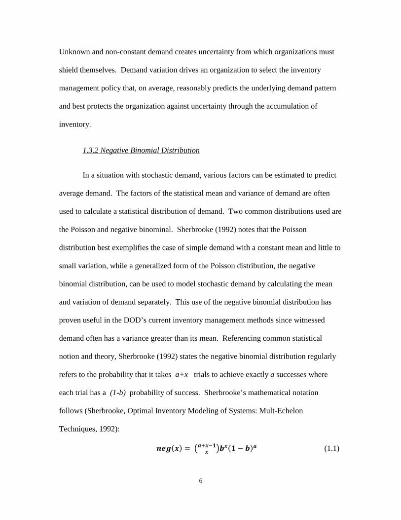
1.3.2 Negative Binomial Distribution
𝒏𝒆𝒈(𝒙) = �𝒂+𝒙−𝟏𝒙 �𝒃𝒙(𝟏 − 𝒃)𝒂 (1.1)
7
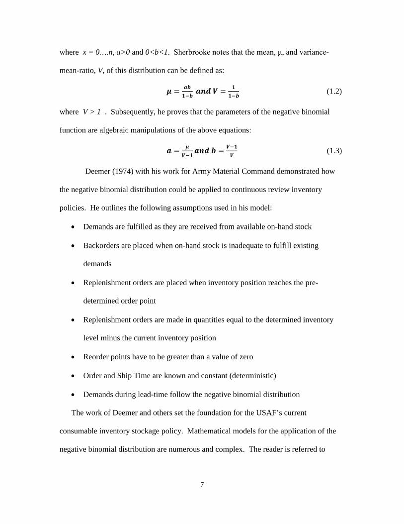
where x = 0….n, a>0 and 0<b<1. Sherbrooke notes that the mean, μ, and variance-
mean-ratio, V, of this distribution can be defined as:
𝝁 = 𝒂𝒃𝟏−𝒃
𝒂𝒏𝒅 𝑽 = 𝟏𝟏−𝒃
(1.2)
where V > 1 . Subsequently, he proves that the parameters of the negative binomial
function are algebraic manipulations of the above equations:
𝒂 = 𝝁𝑽−𝟏
𝒂𝒏𝒅 𝒃 = 𝑽−𝟏𝑽
(1.3)
Deemer (1974) with his work for Army Material Command demonstrated how
the negative binomial distribution could be applied to continuous review inventory
policies. He outlines the following assumptions used in his model:
• Demands are fulfilled as they are received from available on-hand stock
• Backorders are placed when on-hand stock is inadequate to fulfill existing
demands
• Replenishment orders are placed when inventory position reaches the pre-
determined order point
• Replenishment orders are made in quantities equal to the determined inventory
level minus the current inventory position
• Reorder points have to be greater than a value of zero
• Order and Ship Time are known and constant (deterministic)
• Demands during lead-time follow the negative binomial distribution
The work of Deemer and others set the foundation for the USAF’s current
consumable inventory stockage policy. Mathematical models for the application of the
negative binomial distribution are numerous and complex. The reader is referred to
8
Deemer’s work to see how the computational method of recursion applies in this
situation.
In combination, the type and form of an organization’s inventory policy dictates
frequency of inventory reviews, frequency of replenishment orders, and the size of
replenishment orders. These decisions affect how much protection an inventory affords
an organization and its operations from uncertainty. Due to its nature of operations, the
military is often faced with great uncertainty in the accomplishment of its mission. For
this reason, great lengths are taken by the DoD and military services in determining
relevant inventory management strategies.
1.4 Air Force Stockage Policy
The sustainment of USAF flying missions is greatly contingent upon adequate
levels of supporting stock. This supporting stock is made up of two types of stock –
consumables and recoverables. Consumables, as the name implies, are those items that
are consumed in use or cannot be economically repaired (Department of the Air Force
(DAF), 2011:15). Recoverables are those items, that upon failure, have the potential to
be economically repaired (DAF, 2011:15). As the USAF manages each category of items
differently, we will only be addressing its management of consumable items in this
research.
The goal of USAF Stockage Policy is to maximize customer support while
minimizing inventory costs (DAF, 2011:1). USAF stocking decisions are based on the
presence or absence of demand. The absence or presence of demand drives numerous
decision criteria when deciding the range and depth of item stock levels. In the absence
9
of demand, the USAF uses non-demand based stock leveling techniques rooted in the
judgment of subject matter experts to establish and manage stock levels of items. In the
presence of demand, the USAF uses stock leveling techniques whose theories have been
proven through numerous academic and analytical studies. In the context of studying
inventory replenishment strategies at the end of conflict, focus is given to demand-based
stock leveling techniques and their applicable inventory policies towards the management
of consumable items.
In setting stock levels for consumable items on which past demands have been
recorded, the USAF uses past demand data as a predictor of future demand. The USAF
conducts extensive demand and item consumption data collection to determine the most
appropriate stocking actions of an item. At the root of demand-based stocking decisions
lie two fundamental questions – what to stock and how much to stock. The USAF calls
these concepts range (what to stock) and depth (how much of an item to stock) (DAF,
2011:2). An item’s range has to be determined before its depth.
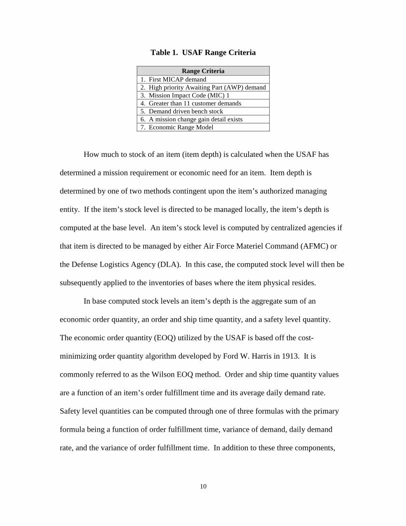
The USAF uses several criteria to determine the range of their inventory (see
Table 1). In keeping with DoD policy, the USAF’s range of inventory items is
determined by mission requirements and/or economic need (DAF, 2011:5). A stock level
will be computed for any item meeting one of seven range decision criteria as specified
by Air Force Manual (AFMAN) 23-110, the USAF Supply Manual.
10
Table 1. USAF Range Criteria
Range Criteria 1. First MICAP demand 2. High priority Awaiting Part (AWP) demand 3. Mission Impact Code (MIC) 1 4. Greater than 11 customer demands 5. Demand driven bench stock 6. A mission change gain detail exists 7. Economic Range Model
How much to stock of an item (item depth) is calculated when the USAF has
determined a mission requirement or economic need for an item. Item depth is
determined by one of two methods contingent upon the item’s authorized managing
entity. If the item’s stock level is directed to be managed locally, the item’s depth is
computed at the base level. An item’s stock level is computed by centralized agencies if
that item is directed to be managed by either Air Force Materiel Command (AFMC) or
the Defense Logistics Agency (DLA). In this case, the computed stock level will then be
subsequently applied to the inventories of bases where the item physical resides.
In base computed stock levels an item’s depth is the aggregate sum of an
economic order quantity, an order and ship time quantity, and a safety level quantity.
The economic order quantity (EOQ) utilized by the USAF is based off the cost-
minimizing order quantity algorithm developed by Ford W. Harris in 1913. It is
commonly referred to as the Wilson EOQ method. Order and ship time quantity values
are a function of an item’s order fulfillment time and its average daily demand rate.
Safety level quantities can be computed through one of three formulas with the primary
formula being a function of order fulfillment time, variance of demand, daily demand
rate, and the variance of order fulfillment time. In addition to these three components,
11
the USAF applies a truncation factor of 0.999 to the computation to upwardly round the
value to the next highest whole number. Base computed stock levels are implemented
through a continuous review inventory policy.
In centrally computed stock levels for items with a demand history, an item’s depth is
calculated using one of two methodologies: Readiness Base Leveling (RBL) or
Customer Oriented Leveling Technique (COLT). The RBL method is used for select
consumable items managed by AFMC, while COLT, the more common of the two
methods, is used to compute stock levels for DLA managed items. Both methodologies
have an objective function that seeks to minimize backorders and customer wait times.
Centrally computed stock levels are implemented through a periodic review inventory
policy implemented by centralized agencies.
First utilized in 2001 by AFMC at the Air Logistics Centers, COLT fundamentally
changed the way the USAF computed consumable stock levels. Before the invention of
COLT, the USAF strictly utilized Harris’s EOQ model to manage consumable items
procured through DLA (Gaudette and others, 2001:4). COLT relaxes the assumptions
made by EOQ model and seeks to minimize customer wait times under pecuniary
constraints. COLT overcomes the following common violations to the EOQ assumptions
through a multi-echelon systems approach that addresses the demand and lead-time
variability commonly observed in today’s supply chain.
• Known and constant lead-time
• Known and constant demand
• Demand independence
• Single echelon supply chains
12
• Known ordering and holding costs
Witnessing the benefits of COLT at the depot levels, AFMC worked with other
USAF major commanders late in the year 2003 to apply the COLT methodology to base
level inventories. The biggest advantage to using COLT at the base level is that it
computationally linked wholesale supply performance data to retail supply requirements
(DAF, 2004:43). COLT achieves this linkage with various factors and a fundamentally
different assumption regarding demand. First, COLT utilizes the percentage of time a
wholesale activity expects to have an item available when requested and the historical
average time a customer has had to wait for a backordered part (Vinson and Gaudette,
2002:19). Secondly, COLT assumes that demand during lead-time is distributed as a
negative binomial random variate (Vinson and Gaudette, 2002:19). This distributional
assumption is based in part on previous data showing that demand variance often exceeds
the mean of demand during lead-time (Deemer, 1974; Vinson and Gaudette, 2002:19).
As stated previously, COLT’s objective function seeks to reduce customer wait
time under fiscal constraints. The initial implementation of COLT was based strictly on
the achievement of a stock level within a fiscal constraint. Due to budgetary processes
and the tendency of the initial COLT model to optimize customer wait time as a function
of inventory investment, stock levels were computed noticeably lower in base level
inventories. Due to the impact of small stock levels at a base, the marginal analysis
method of the COLT method was matured to set stock levels under not only fiscal
constraints but also a predefined target performance objective (DAF, 2004:28). This
target performance objective, known as a sort value, was determined by AFMC to be the
13
most acceptable method in setting stock levels for base inventories. The COLT model is
now used for computing stock levels for DLA consumables at both deployed and home
station locations.
1.5 Problem Statement
As the USAF completes its withdraw from Iraq and sets its focus on the
remainder of operations in Afghanistan, the need for a synchronized plan that best
redeploys equipment while sustaining capabilities in a complex environment will re-
emerge for senior leadership. While variables and factors at the macro-level of
operations will play an enormous role in the demobilization effort, an understanding of
actions at the micro-level of operations will aid in the development of a successful plan.
The goal of this research project is to evaluate the recent supply reduction methods of the
Iraq withdrawal to gain an understanding of consumable inventory management policies
that can be used in future demobilization efforts. In addition, this research attempts to
provide an unbiased evaluation of inventory reduction plans and their impact to mission
accomplishment in contingency situations.
1.6 Research Questions
1. Should drawdowns, at the system level, of inventory at contingency locations be treated any differently than the redistribution of excess inventory at peacetime locations?
2. Is there a statistical and/or practical difference among policies for reducing
inventory levels in the final phases of a contingency operation?
14
3. What are appropriate measures to be used in evaluating policies for drawdown of inventory in a contingency environment?
4. What parameters should guide inventory drawdowns in future contingency
operations?
1.7 Scope and Limitations
The investigative questions posed above are only a subset of the range of
questions that can be addressed with the appropriate simulation model. Simulation
models are appropriately suited for this research as there is no simple analytical model
and the real world system has complex interactions and interdependences that make it
challenging to understand macro-level results (Carson, 2005: 17). The purpose of this
project is to evaluate past inventory management actions in the hopes of developing new
theories and guidelines of inventory management for use during the phases of
contingency operations.
1.8 Outline
Chapter 2 provides a detailed description of model development along with
pertinent information of input data modeling and output analysis. Chapter 3 is an
application of the model to the case study of the Balad AB drawdown plans along with
results. Chapter 4 concludes the thesis by discussing significant findings and providing
recommendations for future research. Chapters 2 and 3 are structured as an individual
journal paper and conference proceedings.

15
2. Simulation of Base Stock Level Reduction for an Overseas Contingency
Operating Base
2.1 Introduction
Outdated supply strategies and the USAF’s continued presence in Saudi Arabia
after the first Gulf War gave cause to the recommendation of new supply processes in
support of sustainment operations at contingency locations (Hunt, 2011). With the
conclusion of the Gulf War, the USAF again faced a situation where lagging supply
strategy caused the redeployment of equipment to be conducted hastily with an enormous
amount of work levied upon those stateside supply professionals who received the
equipment (Fulk D. A., 2011). During the war in Iraq, supply support strategies
developed after the conclusion of sustainment operations in Saudi Arabia were
implemented with success. Contrasting to this success was the fact that USAF supply
professionals were faced with the challenge of moving years’ worth of inventory out of a
war zone yet again.
To prevent the situation that occurred in Saudi Arabia, the Global Logistics
Support Center (GLSC) developed a plan that would gradually reduce supply levels and
systematically convert sustainment levels of inventory back to expeditionary levels. The
goals behind this plan were threefold: ensure the preservation of equipment
accountability, maximize weapon system availability to the very end of operations, and
support an efficient and effective base closure effort (Fulk, 2010). The computational
methods behind this planned drawdown assumed a linear decreasing trend in demand that
would require support up until a time where it would be feasible to support requirements
16
out of readiness spare kits (RSP). Upon gaining agreement on the plan with Air Force
Central Command (AFCENT), GLSC’s lead unit, the 735th Supply Chain Operations
Group (SCOG), implemented their plan against Balad AB’s inventory. The developed
plan performed within expectations up until a decision was made by the Air Staff, with
AFCENT concurrence, to immediately zero out stock levels on items that either had not
caused a non-mission-capable for supply (NMCS) event in the past or had previously
caused a NMCS event but maintained a zero on-hand balance as of the date of the
decision. These items are identified in the USAF’s supply system with a mission impact
code (MIC) of 1 and are commonly referred to as MIC-1 items.
The situation and decisions regarding the plan to reduce inventory at Balad AB
presents unique opportunity to study different facets of inventory management policy.
Analytically, the plan presents a situation in which USAF inventory management policies
could be evaluated under the assumption of a linear decreasing trend in demand. The
situation also brings up strategic considerations surrounding inventory management
policies and processes in the redeployment phase of contingency. The solutions are at
best estimations due to the fact that developed plans were not carried through to the
closure of Balad AB. It is the clarification and development of estimations and
assumptions into strategies and policies that will aid supply support strategies in future
redeployments. An agent-based model simulating Air Force inventory management
policies was developed to compare and contrast the planned and implemented inventory
reduction techniques.
17
2.2 Overview
This research develops an agent-based simulation model of the retail supply chain
supporting Balad AB during its closure. The success of a supply chain, especially one
which supports deployed warfighters, depends upon the interactions of many different
complex processes and systems. Abstractions of four inventory management processes
are used in this research to evaluate the inventory reduction plans used during Balad
AB’s closure and to broaden the understanding of feasible strategies that could be utilized
to reduce the inventory of a contingency operating base back to expeditionary levels.
The first process conceptualizes how demands are placed on the supply chain at the air
base. The second process of the model represents the processing and fulfilling of
customer demands by a supporting primary operating stock (POS) and deployed RSP
inventories. The third process abstracts the logic of USAF inventory management
computations. Finally, the fourth process generalizes the resupply of inventory levels at
the deployed operating base.
The use of agent-based modeling to study inventory reduction is an untested
approach. Many academic studies in the analytical fashion have attempted to determine
an optimal algorithm that would best reduce inventories under the assumption of linear
decreasing demand – see Barbosa and Friedman (1979); Ramani and Venkatraman
(1988); Hill, Omar and Smith (1999); and Zhao, Yang and Rand (2001). All of these
authors seek to determine the optimal point at which the stocking of inventory should be
suspended in order to minimize ordering and replenishment costs while still maintaining
an acceptable degree of service. The approach in this research is not to determine that
18
optimal point, but to understand the characteristics of decreasing demand in order to
increase the depth of knowledge regarding wartime supply strategies. The use of
simulation is very applicable to this topic since the application of different policies and
the study of their respective impact on the overall system cannot be achieved without
incurring great opportunity and pecuniary costs. Banks and others (2010) defend the use
of simulation in decision-making when the experimentation of new designs or policies
can take place before their implementation in order to investigate and gain insight into
potential outcomes. Hence the use of a simulation model for evaluating and studying the
differing inventory reduction plans at Balad AB.
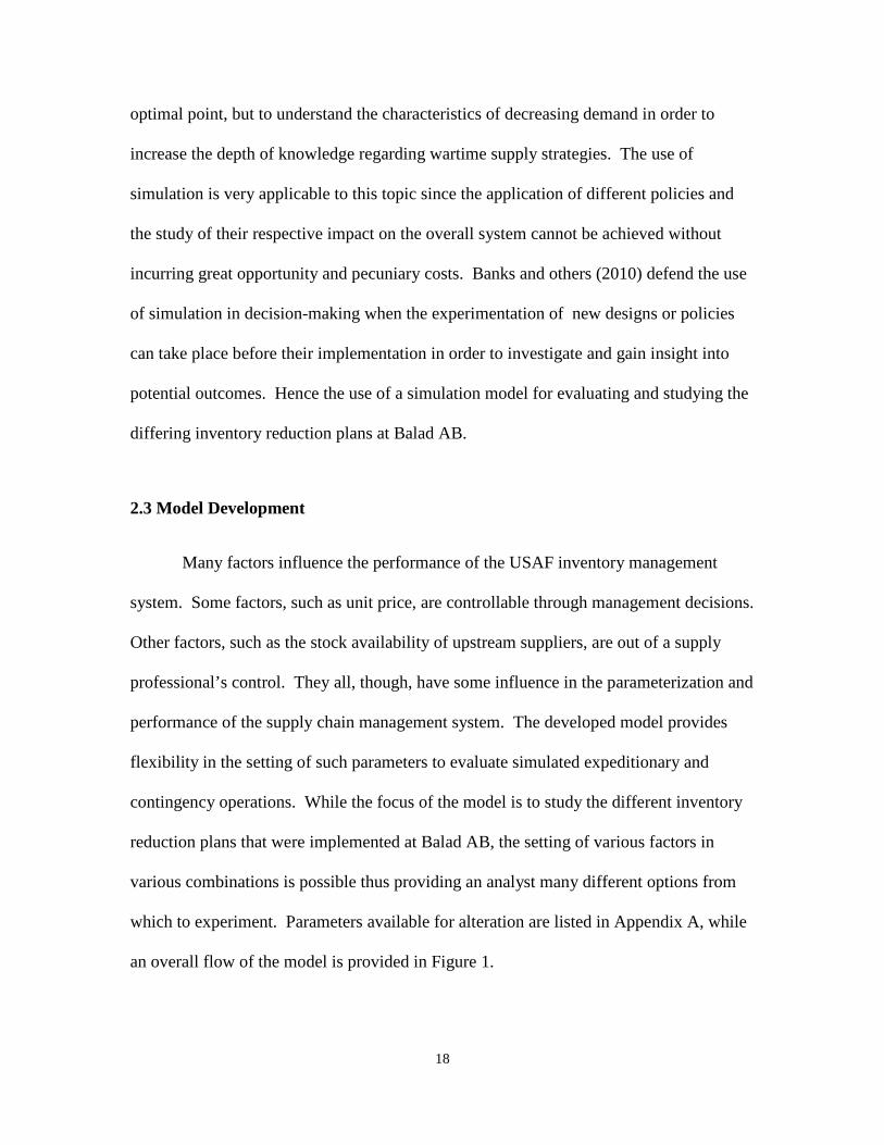
2.3 Model Development
Many factors influence the performance of the USAF inventory management
system. Some factors, such as unit price, are controllable through management decisions.
Other factors, such as the stock availability of upstream suppliers, are out of a supply
professional’s control. They all, though, have some influence in the parameterization and
performance of the supply chain management system. The developed model provides
flexibility in the setting of such parameters to evaluate simulated expeditionary and
contingency operations. While the focus of the model is to study the different inventory
reduction plans that were implemented at Balad AB, the setting of various factors in
various combinations is possible thus providing an analyst many different options from
which to experiment. Parameters available for alteration are listed in Appendix A, while
an overall flow of the model is provided in Figure 1.
19
Agents Generate DemandRate ~E(DDFR)
Size~NBD(DDR/DDFR,VOD)
Can ELRS Fulfill Demand?
Send Backorder to SoS
Can SoS fulfill ELRS Order
Fulfill Agent Demand
Fulfill ELRS Order
Send order to Tier 1 Supplier
Yes
Yes
No
No
Capture Demand and Order Statistics
Calculate/set levels using COLT
or EOQ depth methods
Closure Method Set?
No
Set levels by Max ASL or EDQ
methodYes
AcronymsASL – Adjusted Stock LevelDDFR – Daily Demand Frequency RateDDR – Daily Demand RateEDQ – Expected Demand QuantityELRS – Expeditionary Logistics Readiness SquadronE(DDFR) – Expected Value of DDFRNBD - Negative Binomial DistributionSoS – Source of SupplyVOD – Variance of Demand
Figure 1. General Model Flow
North and Macal (2007) state that a model’s execution time of a simulation can be
divided into two phases – the total time simulated (execution horizon) and the period
applicable to answering questions and assisting decision making (guidance horizon). The
period within the execution horizon, but outside the guidance horizon is commonly
referred to as the initialization period. The initialization period allows the model to
remove any bias from starting the system empty and idle. The developed model for this
thesis has a static execution horizon of 27 months and a dynamic guidance horizon that
can be set before the model’s execution. A simulation execution horizon of 27 months
was chosen to allow for an adequate initialization period that can be set by the analyst. A
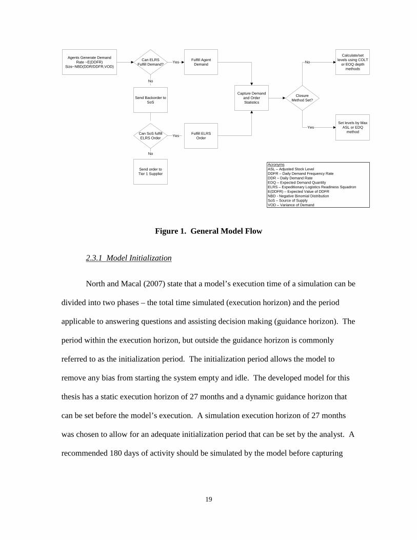
recommended 180 days of activity should be simulated by the model before capturing
2.3.1 Model Initialization
20
data for analysis to allow a substantial amount of demand to have been processed through
the system (see Figure 2).
Figure 2. Demand Behavior of Developed Model over Time
GLSC’s plan developed for Balad AB was a 14-month drawdown plan that would
remove all POS inventory from the base’s retail system two months before the base
closing (Fulk, 2010). Given the high variability of the simulation’s initial start-up period
and the fact that asset levels are updated quarterly (DAF, 2011), an initialization period of
no less than 400 days’ worth of simulated time is recommended (see Figure 2). This
initialization period allows a sufficient number of demands to be generated and the
accurate calculation of demand levels and reorder points when using either base or
central computation methods.
The occurrence of requirements on an inventory system, demand, has often been
modeled as discrete probability distribution in simulation models. This event is often
looked at holistically rather than from the perspective of the individual or entity
generating a demand. The developed model takes a scalable approach to generating
demand by allowing agents to place requirements on the inventory system independently
2.3.2 Demand Generation
21
of each other. Each agent generates a demand based on a statistical distribution. The
total demands placed on the system are a function of demands placed by all agents. The
use of agents in this manner deviates from some of the standard agent characteristics that
Macal and North consider such as:
• An agent interacts with other agents
• An agent is situated in an environment where it can interact with other
agents
• An agent can have goal-directed behaviors
• An agent has the ability to learn and adapt its behaviors based on its
experience with the external environment.
Macal and North (2008), though, state that agents do not necessarily need to
possess all of these characteristics to be considered an agent-based model. The
methodology by which agents are used in this model doesn’t necessary preclude the
model from being considered agent-based as Chan et al (2010) point out that agent-based
simulation is usually a hybrid model consisting of discrete events generated by
autonomous objects (agents). The ability of the agents to simultaneously and
independently place demands is what makes agent-based modeling and simulation a
powerful tool to understanding the research under question (Chan et al, 2010). The use
of a fleet size parameter in the model provides scalability to the model by allowing the
population of agents placing demands to be set between a value of one, a single aircraft,
and 36, a multiple of either a six or twelve aircraft unit type code tasking requirement.
Demands for two parts are generated at a frequency described by each part’s daily
demand frequency rate (DDFR) and at a random size based off the part’s daily demand
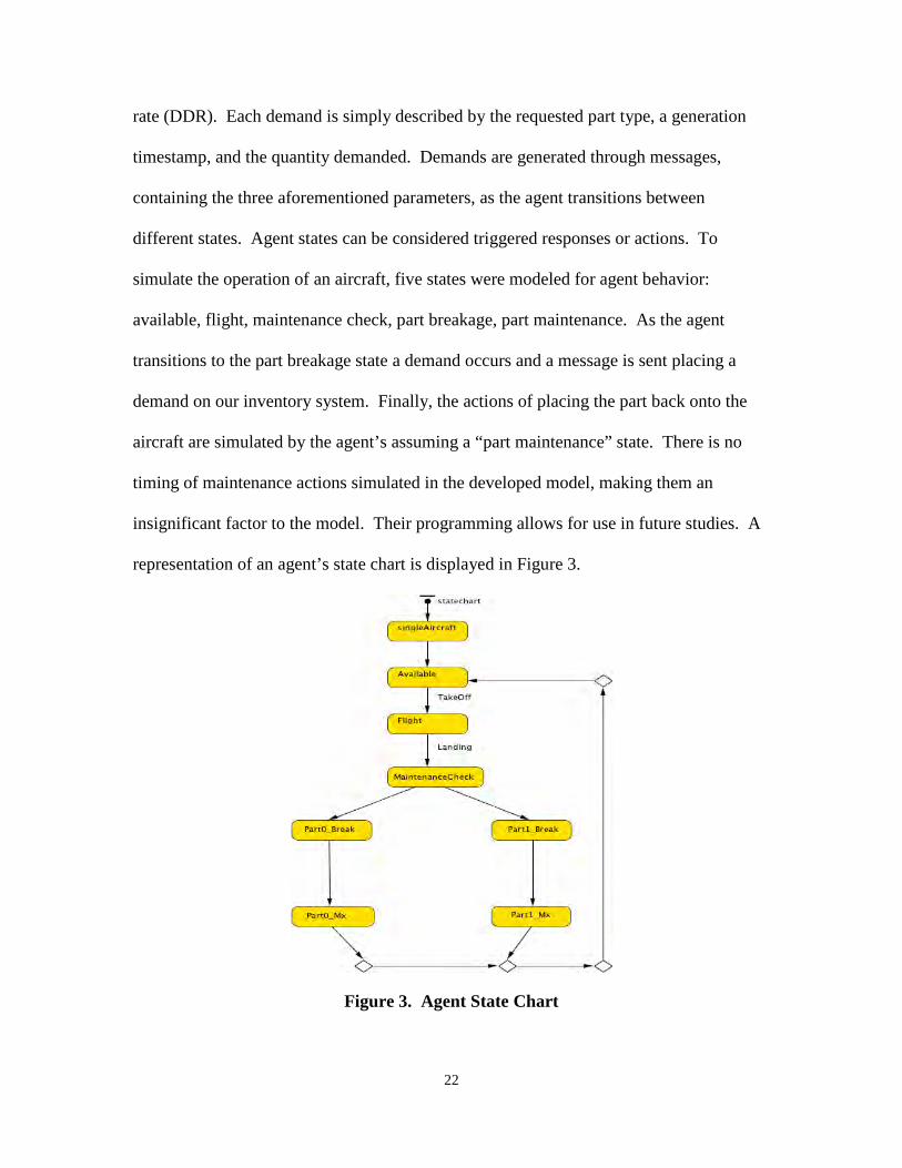
22
rate (DDR). Each demand is simply described by the requested part type, a generation
timestamp, and the quantity demanded. Demands are generated through messages,
containing the three aforementioned parameters, as the agent transitions between
different states. Agent states can be considered triggered responses or actions. To
simulate the operation of an aircraft, five states were modeled for agent behavior:
available, flight, maintenance check, part breakage, part maintenance. As the agent
transitions to the part breakage state a demand occurs and a message is sent placing a
demand on our inventory system. Finally, the actions of placing the part back onto the
aircraft are simulated by the agent’s assuming a “part maintenance” state. There is no
timing of maintenance actions simulated in the developed model, making them an
insignificant factor to the model. Their programming allows for use in future studies. A
representation of an agent’s state chart is displayed in Figure 3.
Figure 3. Agent State Chart
23
In the developed model, all demand fulfillment logic is executed by the entity
labeled ELRS (Expeditionary Logistics Readiness Squadron). The ELRS entity is a java
active object that receives messages from agents and either fulfills the agents’ demands
or queues the agents’ demands when insufficient stock is present in the inventory. Logic
within the ELRS object is constantly run on a simulated daily basis to process agent
demands. Demand fulfillment is executed through the utilization of two sources of stock
- the POS inventory and the RSP inventory. The POS inventory is always checked for
parts before the RSP inventory.
2.3.3 Demand Receipt and Stock Issue Process
Upon receiving an agent demand, the logic within the ELRS object will first
check the inventory levels of its POS. If enough stock is present in the POS, then the
demand is fulfilled completely from this source of parts. If the inventory levels of the
POS are insufficient in fulfilling the entire demand quantity, the stock issue logic satisfies
the demand by issuing then remaining on-hand stock in the POS inventory and then
fulfilling the delta of demand with on-hand stock from the RSP inventory. If unable to
issue any stock from POS, the RSP inventory is used to fulfill the agent demand.
Common to the issue logic for the POS, logic for issues from the RSP will fulfill as much
of the demand quantity as possible. If the inventory position of a part is at such a status
where current on hand stock in either the POS or RSP inventory cannot meet current and
future demands, then a backorder is queued for the demand. A flowchart for the receipt
of demand and stock issuing logic can be found in Appendices B and C.
24
The computation of consumable stock levels can occur through two different
methods, each executed by one of four events. In the initialization of the model, the
analyst selects either standard base computations for stock levels or the Customer
Oriented Leveling Technique (COLT) marginal analysis method utilized by AFMC in the
calculation of consumable stock levels. The model will use the selected technique to
compute consumable item stock levels at the following events.
2.3.4 Computation of Consumable Stock Levels
• Initial level computation executed on the 30th day of simulated time.
• Anytime the inventory position is less than or equal to the item’s reorder point
and the amount of change equals or exceeds thresholds defined by the “Square
Root” rule in AFMAN 23-110, Volume 2, Part 2, Chapter 19, Attachment 19B-
21.
• At the simulated times of 1 Jan, 1 Apr, 1 Jul and 1 Oct to represent the quarterly
update of stock levels.
• At monthly intervals when a closure method has been selected by the analyst
during the initialization of the model.
The standard base computations in the model involve traditional equations for
economic order quantity, order and ship time quantity and safety level quantities. The
variance equations for demand and order and ship time specified in AFMAN 23-110 have
been coded in the model as well. The coding for these equations can be found in
Appendix J.

25
The COLT method compares the calculation of expected backorders for each item
given the demand for the items and conducts a marginal analysis of the two items,
increasing the reorder point of the item that produces the largest marginal benefit in the
reduction of expected backorders. The coding for the COLT method assumes a negative
binomial distribution of expected backorders and conducts a marginal analysis method
with a sort value target equal to the one dated 25 Mar 2011 for Balad AB. For an in-
depth explanation of the application of the negative binomial distribution with respect to
backorders and the COLT methodology the reader is referred to articles by Deemer
(1974), Fulk et al (2006) and Vinson (2002). The coding for the negative binomial
distribution of backorders and the COLT marginal analysis method can be found in
Appendices L and M.
The simulated supply chain creates customer backorders as necessary when
requirements cannot be met with on-hand stock from either the POS or RSP inventory
(DAF, 2011). The developed model will only create a customer backorder when the
combined stock levels of the POS and RSP inventories are insufficient in meeting the
requirement. The model simulates backorders by replacing the demand quantity in the
original demand request with a quantity equal to the delta of unfilled demand. This
precludes the model from placing another demand on the system. If an agent’s demand is
partially filled, the original demand is replaced by a demand equal in size to what remains
to be fulfilled for the agent. An agent’s demand is only deleted from the model when it is
fulfilled in its entirety.
2.3.5 Backorder Processing
26
The replenishment process of the model replicates the described continuous
review inventory replenishment model in AFMAN 23-110, Volume 2, Part 2, Chapter 19,
Attachment 19D-1. On a daily basis, the model conducts a continuous review of its
inventory levels to determine each part’s inventory position. The inventory position of a
part is equal to the sum of on hand quantities in both the POS and RSP inventories and
any quantity of the part already on order minus any quantity of the part on backorder.
Whenever the inventory position for an item is less than or equal to the reorder point
calculated by the model, the logic in the ELRS active object generates a stock
replenishment order there by “pulling” inventory from the source of supply (DAF, 2011).
The amount required for replenishment is equal to the total base need minus the inventory
position (DAF, 2011). Stock replenishment orders take the form of messages passed
between the ELRS active object and the SoS (Source of Supply) active object. The SoS
could represent any source of supply for parts, but in this study it represents the Defense
Logistics Agency (DLA). Replenishment order messages contain a numerical identifier
for the part requested and the replenishment order quantity. Each time a replenishment
message is generated, the time and amount of the order are captured for statistical
measures of order and ship time. A flow chart for the stock replenishment logic and the
associated java code can be found in Appendix E.
2.3.6 Replenishment Process
When an inventory reduction method has been selected in the model and aircraft
are present, the ELRS object will initiate excess stock shipments anytime the on hand
2.3.7 Excess Stock Shipment Process
27
quantity of POS for a part exceeds a newly computed order up-to-level during the
specified drawdown period. This logic simulates the shipment of excess stock off the
base during redeployment operations at a contingency location. If aircraft remain in the
model when a newly computed POS level creates an excess shipment, the model logic
will “ship” the quantity of stock above the newly computed POS level. If no aircraft are
present in the model when a newly computed POS level creates an excess shipment, the
model logic will first fill any stock level deficiency in the RSP and then “ship” any
remaining excess POS inventory. These transactions are captured in the model’s output.
Logic for the creation of excess shipments and accompanying java code is presented in
Appendix F.
Two inventory reduction methods are presented in the model. One is based on the
setting of non-demand-based stock levels for POS inventory. AFMAN 23-110 describes
the policy of setting non-demand-based stock levels as a way of establishing sufficient
stock levels in situations where historical demand patterns are not reasonable estimations
of future demand patterns (DAF, 2011). The other method available for selection models
the formula developed by the 735th SCOG to linearly decrease stock levels. This
method, referred to as expected demand quantities, calculates stock levels as a function of
the item’s daily demand rate and the time left until base closure. For ease of reference,
this plan will be referred to as the “EDQ” plan. The developed model allows the analyst
to select the inventory reduction method and a start date for it to be implemented.
2.3.8 Inventory Reduction Methods
28
The settings of non-demand-based stock levels are a way to adjust stock levels
based on the assumption that past demand is not a predictor of future demand. The
method is referred to as adjusted stock levels (ASLs). The USAF has developed three
different types of ASLs to adjust supply support against changing levels of customer
demand: minimum, maximum, and fixed. Of the three, the setting of maximum ASLs
are used in this model as it was the decision by Air Staff to set maximum ASLs on non-
MIC-1 and MIC-1 assets with zero on-hand balances. Maximum ASLs act as stockage
ceilings in that they restrict computed stock levels to a specified level. In the case of
Balad AB’s closure, maximum ASLs on the POS inventories of non-MIC 1 and MIC-1
items with zero on-hand balances were set to a value of zero (Fulk D. A., Balad Levels
Drawdown Plan, 2011). This particular application of applying maximum ASLs on
Balad AB’s POS effectively zeroed out demand levels and reorder points on those items
identified under this plan. This policy is demonstrated in the model by zeroing out an
item’s level at the time specified during the initialization of the model. For future
reference, this plan will be referred to as the “Maximum ASL” plan. The flowchart and
java logic for this inventory reduction plan can be found in Appendix Q.
The EDQ plan developed by the 735th SCOG was based on a formula of expected
demand that calculated expected future demands as a function of an asset’s DDR and the
remaining time of base operations. The expected demand formula is similar to a mission
change DDR (MCDDR) that is used by stateside bases undergoing increases or decreases
in the inventory of an assigned weapon system, but it doesn’t utilize sortie information as
in the MCDDR calculations. The expected demand formula simply applies the remaining
time in a finite horizon to an item’s DDR under the assumption that demand on an asset
29
and thus its DDR would decrease in a linear fashion as operations scale back. It should
be noted that this plan assumed at least some correlation between past demand and future
demand. The parameters of the formula zero out POS levels two months prior to the
closure of the base or when aircraft no longer remain present in the model. It is at this
time when any further operations were assumed to be supported out of RSP inventories.
Special rounding rules were to have been applied to keep stock available as the time
horizon for Balad AB’s closure decreased. Model logic and implemented code can be
found in Appendix Q.
In order to maintain a focus on the research in question, various assumptions were
made that influenced model development. In addition to assumptions specified by
Deemer (1970) when studying continuous review inventory policies, the following key
assumptions were made:
2.3.9 Assumptions
• Data obtained through AFLMA, the GLSC, and LIMS-EV is accurate and
complete.
• Demand interarrival times are assumed to be an exponentially distributed function
of the item’s daily demand frequency rate (DDFR) divided by a denominator
equal to the average amount of aircraft flying sorties from Balad AB on 25 Mar
2011.
• Demand size is assumed to be distributed according to the negative binomial
function with a variance calculated using the variance of demand (VOD) formula
specified by AFMAN 23-110.
30
• RSP demand levels are non-demand based and POS levels are demand based.
The RSP levels do not represent the actual levels of the items in RSP kits at Balad
AB, but are modeled to provide a sense of realism in the model.
• Bench stock is not explicitly modeled and assumed part of the POS inventory.
• No cannibalization, lateral resupply or local sourcing of parts. All parts are
sourced from the designated source of supply.
• No commonality exists among parts for different weapon systems.
• Delays for inbound transportation of stock are modeled at two levels, but no delay
exists for transportation of stock off base.
• RSPs are filled with any excess items from the POS inventory during the
drawdown phase of the base.
• RSPs remain at the contingency location until the end of the drawdown.
• No gaps in time between deployment of like MDSs at the location.
• A finite planning horizon that ends with date specified for the withdrawal of U.S.
forces from Iraq.
2.4 Supporting Data
Key to structuring the experiment for this research was being able to categorically
define differing levels of demand and unit price, in addition to obtaining relative
consumption and leveling information for all consumable items stocked at Balad AB.
The following data sources were used to capture data pertinent to the model’s input
parameters.
31
• A COLT input file (n = 9,975), dated 25 Mar 2011, obtained from the 735th
SCOG by way of the 402nd SCMS at Wright Patterson AFB
• A LIMS-EV download of the item records for all inventory stock at Balad AB on
25 Mar 2011 (n = 33,257)
• An RSP detail listing for items in High Priority Mission Support Kits at Balad AB
on 25 Mar 2011(n = 19,968)
• An inventory transaction history report, obtained from LIMS-EV, of all issues and
due-outs at Balad AB between the dates of 25 Sept 2009 and 25 Mar 2011
(n=23,071)
Total records from all combined data sets equaled 86,271, but not all records were
pertinent to the research. Records had to be categorized, filtered, and linked to obtain a
final data set that represented currently demanded DLA-managed consumable items
supported by RSP inventories. To provide insight on how the final data set was obtained,
a brief description of how data was categorized, filtered and linked is provided.
The data filtering and consolidation of information was made possible by using
the Microsoft Access software program to the link the different data sources and querying
for specific data points. Of the 33,257 item records captured for Balad AB, only 25,580
were items with a expendability-recoverability-reparability code of XB3 and a budget
code of 9 (consumable item). Of those items identified as a consumable items, 91% (n =
23,192) had a routing identifier code classifying DLA as the source of supply and of
those items only 8,318 had some type of demand registered in the previous 18 months.
2.4.1 Resulting Data Set
32
When linking these 8,318 records to the 735th SCOG’s COLT input file and to the RSP
detail listing, the resulting dataset numbered 4,842 item records. Filtering was applied to
this data to narrow our final data set to a predetermined supported mission design series,
F-16 aircraft. The resulting data set numbered 1,166 records. These item records were
then divided between MIC-1 and non-MIC 1 records to achieve a commonality to the
inventory drawdown situation at Balad AB.
Being able to categorically assign items to different categories of demand
frequency, demand size and unit price was necessary to the research’s experiments.
Categorical assignment of data was conducted on the 8,318 records identified as DLA-
managed consumable items possessing some type of registered demand in the previous
18 months. Categories for demand frequency, demand size and unit price were
determined by ranking that relative factor in relation to every other item and then
dividing items based on quartile boundaries as shown in Table 2. For example with this
methodology all items with a relative factor ranking between and including a value 1 and
2080 were put in the “Low” category.
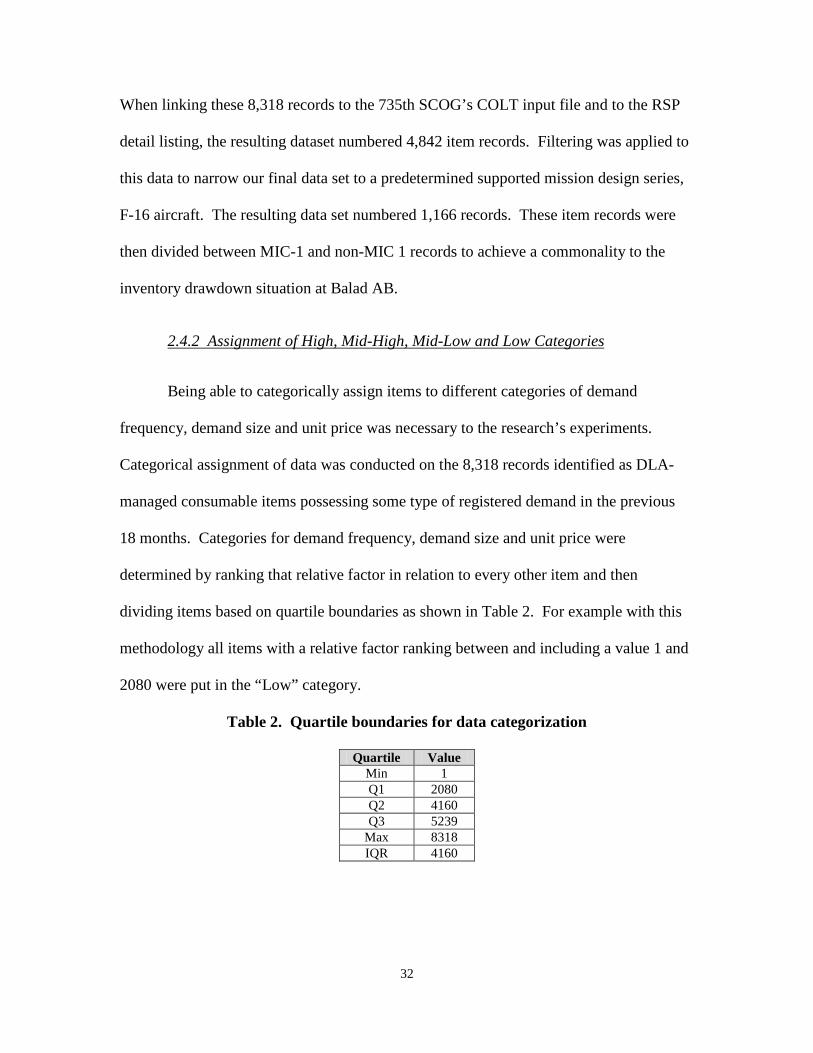
2.4.2 Assignment of High, Mid-High, Mid-Low and Low Categories
Table 2. Quartile boundaries for data categorization
Quartile Value Min 1 Q1 2080 Q2 4160 Q3 5239
Max 8318 IQR 4160

33
The categorical assignment of demand frequency was made possible by
computing an item’s DDFR from data provided in an item’s record. DDFR is a
quantitative calculation that captures the daily average of requests for a certain item
(DAF, 2011). The use of DDFR allows for the determination of how fast demands arrive
into the supply system. Essentially, it is an 18-month moving average, but its formula
involves the use of three moving windows of time. It is calculated by dividing the
aggregate sum of demands occurring in three rolling window periods –the current six
month period, ND(CP); seven and 12 months ago, ND(1PSM); 13 and 18 months ago,
ND(2PSM) – by a time period defined by as the difference between the current date (CD)
and the item’s date of first demand (DOFD). The denominator of this formula has a
minimum value of 365, to ensure that at least 2 customer demands register a significant
value, and a maximum value of 540. The formula for DDFR is (ND(2PSM) +
ND(1PSM) + ND(CP))/(CD – DOFD) .
2.4.3 Categorical Assignment of Demand Frequency Rates
The number of demands in each period and the DOFD were obtained using data
provided in an item’s record. The date of 25 Mar 2011 was used as the current date since
the item record was pulled for that date. Using these pieces of information, a DDFR was
computed for all consumable items. Using categories based off of the previously
described quartile computations, all consumable items were divided into four categories –
high, mid-high, mid-low, and low. These four categories provided a simple, yet
effective, way to categorically assign the frequency of demands for an item. The

34
quartiles, categorical assignments, and simple descriptive statistics for demand frequency
rates for the 8,138 demanded DLA-managed consumable items are provided in Table 3.
Table 3. Quartile, Categorical Assignment and Descriptive Statistics for DDFR
Categorical Assignment Daily Demand Frequency Quantile Item Count Grouping Max μ Min σ
Min <= x <= 2080 2080 Low 0.0019 0.0019 0.0018 0.0000 2081 <= x <= 4160 2080 Mid-Low 0.0027 0.0024 0.0019 0.0003 4161 <= x <= 6239 2079 Mid-High 0.0051 0.0034 0.0027 0.0006 6240 <= x <= 8318 2079 High 0.1238 0.0103 0.0051 0.0092
The categorical assignment of demand size was made possible by computing an
items’ DDR from data provided in an item’s record. DDR is a quantitative calculation
that computes the average quantity of an item demanded daily. It allows for the
determination of the size of each arriving demand into the supply system. DDR is
calculated by dividing the total quantity of an item requested, known as the cumulative
recurring demand (CRD) factor, over a time defined by subtracting an item’s DOFD from
the current date. The minimum amount of time used in the DDR computation is
constrained to 180 days, while the maximum time is set to 540 days. Due to an
annualization process conducted in the months of September and March, the CRD
quantity of an item is always based on the most recent 365-day period. In addition, an
item’s DOFD is also annualized at the same time by resetting it to a date 365 days before
the date of the annualization process. The formula calculating an item’s DDR is
CRD/(CD-DOFD) .
2.4.4 Categorical Assignment of Demand Size
35
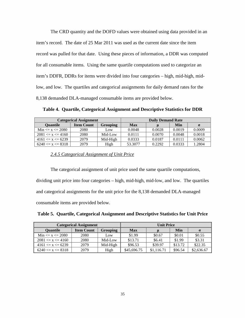
The CRD quantity and the DOFD values were obtained using data provided in an
item’s record. The date of 25 Mar 2011 was used as the current date since the item
record was pulled for that date. Using these pieces of information, a DDR was computed
for all consumable items. Using the same quartile computations used to categorize an
item’s DDFR, DDRs for items were divided into four categories – high, mid-high, mid-
low, and low. The quartiles and categorical assignments for daily demand rates for the
8,138 demanded DLA-managed consumable items are provided below.
Table 4. Quartile, Categorical Assignment and Descriptive Statistics for DDR
Categorical Assignment Daily Demand Rate Quantile Item Count Grouping Max μ Min σ
Min <= x <= 2080 2080 Low 0.0048 0.0028 0.0019 0.0009 2081 <= x <= 4160 2080 Mid-Low 0.0111 0.0070 0.0048 0.0018 4161 <= x <= 6239 2079 Mid-High 0.0333 0.0187 0.0111 0.0062 6240 <= x <= 8318 2079 High 53.3077 0.2292 0.0333 1.2804
The categorical assignment of unit price used the same quartile computations,
dividing unit price into four categories – high, mid-high, mid-low, and low. The quartiles
and categorical assignments for the unit price for the 8,138 demanded DLA-managed
consumable items are provided below.
2.4.5 Categorical Assignment of Unit Price
Table 5. Quartile, Categorical Assignment and Descriptive Statistics for Unit Price
Categorical Assignment Unit Price Quantile Item Count Grouping Max μ Min σ
Min <= x <= 2080 2080 Low $1.99 $0.67 $0.01 $0.55 2081 <= x <= 4160 2080 Mid-Low $13.71 $6.41 $1.99 $3.31 4161 <= x <= 6239 2079 Mid-High $96.53 $39.97 $13.72 $22.35 6240 <= x <= 8318 2079 High $45,696.75 $1,116.71 $96.54 $2,636.67
36
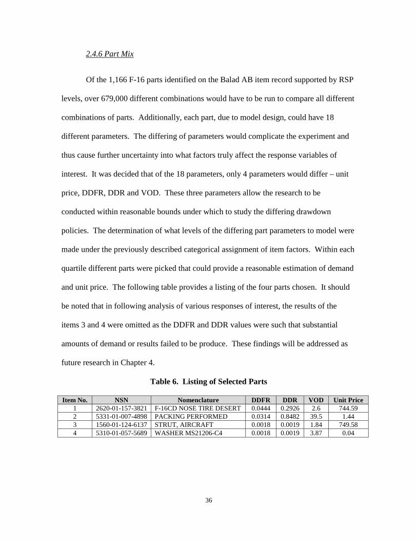
Of the 1,166 F-16 parts identified on the Balad AB item record supported by RSP
levels, over 679,000 different combinations would have to be run to compare all different
combinations of parts. Additionally, each part, due to model design, could have 18
different parameters. The differing of parameters would complicate the experiment and
thus cause further uncertainty into what factors truly affect the response variables of
interest. It was decided that of the 18 parameters, only 4 parameters would differ – unit
price, DDFR, DDR and VOD. These three parameters allow the research to be
conducted within reasonable bounds under which to study the differing drawdown
policies. The determination of what levels of the differing part parameters to model were
made under the previously described categorical assignment of item factors. Within each
quartile different parts were picked that could provide a reasonable estimation of demand
and unit price. The following table provides a listing of the four parts chosen. It should
be noted that in following analysis of various responses of interest, the results of the
items 3 and 4 were omitted as the DDFR and DDR values were such that substantial
amounts of demand or results failed to be produce. These findings will be addressed as
future research in Chapter 4.
2.4.6 Part Mix
Table 6. Listing of Selected Parts
Item No. NSN Nomenclature DDFR DDR VOD Unit Price 1 2620-01-157-3821 F-16CD NOSE TIRE DESERT 0.0444 0.2926 2.6 744.59 2 5331-01-007-4898 PACKING PERFORMED 0.0314 0.8482 39.5 1.44 3 1560-01-124-6137 STRUT, AIRCRAFT 0.0018 0.0019 1.84 749.58 4 5310-01-057-5689 WASHER MS21206-C4 0.0018 0.0019 3.87 0.04
37
Individual demand sizes are assumed to follow a negative binomial distribution
whose mean is equal to a part’s DDR divided by its DDR and whose variance is equal to
the VOD value calculated from the 25 March 2011 item record. Since a part’s DDR is a
measure of the quantity of the item used daily dividing this by DDFR gives a reasonable
approximation of individual demand size. The VOD of an item is calculated using three
factors – an item’s cumulative demand quantity (CDQ) , cumulative demand quantity
squared (CDQ2) and the number of days since the item’s DOFD. An item’s CDQ value
is number of item units ordered by a customer, while an item’s CDQ2 value is the sum of
all CDQ squared values (DAF, 2011). An item’s CDQ value is collected separately from
an item’s CRD value even though they both represent the same data due to a difference in
the date at which CDQ data collection started (DAF, 2011). Representative examples of
these calculations are represented equations 2.1 and 2.2.
2.4.7 Modeling Demand Size
𝑬(𝑫𝒆𝒎𝒂𝒏𝒅 𝑺𝒊𝒛𝒆) = .𝟖𝟒𝟖𝟐 𝒖𝒏𝒊𝒕𝒔 𝒅𝒆𝒎𝒂𝒏𝒅𝒆𝒅𝟏 𝒅𝒂𝒚
÷ .𝟎𝟑𝟏𝟒 𝒅𝒆𝒎𝒂𝒏𝒅𝒔𝟏 𝒅𝒂𝒚
≅ 𝟐𝟕 𝒖𝒏𝒊𝒕𝒔/𝒅𝒆𝒎𝒂𝒏𝒅 (2.1)
𝑽(𝑫𝒆𝒎𝒂𝒏𝒅 𝑺𝒊𝒛𝒆) = 𝑪𝑫𝑸𝟐−𝑪𝑫𝑸
𝟐
𝒏𝒏
=𝟐𝟏,𝟕𝟔𝟒−𝟒𝟓𝟖
𝟐
𝟓𝟒𝟎𝟓𝟒𝟎
≅ 𝟑𝟗.𝟓 (2.2)
The model was run over different sizes of supported aircraft fleets – 12, 24, 36.
Multiples of twelve were used to represent differing numbers of standard six-ship
deployment packages. Historical sortie data for Balad AB identifies an average of 24
aircraft flying sorties into and out of Balad AB from Jan 2009 to October 2010. Using
2.4.8 Fleet Sizes
38
this data, fleet sizes of 12, 24, and 36 were selected to provide a representative number of
aircraft supported during the drawdown phase of a base.
The two drawdown policies were implemented at differing times as demonstrated
in Figure 5. Within the context of this experiment, the commonality of time between the
two plans is important to the understanding of which drawdown plan performs better
under similar circumstances. Comparing EDQ plan 14 months out from base closure
against the Maximum ASL plan 9 months out from Balad AB’s closure would constitute
an unacceptable level of comparison. To gain commonality over measures of
performance, data was only captured during the simulation time representing the period
from March 2011 to December 2011. Capturing data earlier than this period could
possibly skew the results towards a favoring of the maximum adjusted stock level plan
even though it wasn’t implemented until March 2011.
2.4.9 Period of Study
Additionally, the period of study covers different drawdown timelines of aircraft.
Aircraft in the model redeploy according to one of two timelines, 6 or 12 months, and at a
whole integer factor that would result in zero aircraft remaining the end of a model
replication. For example, a fleet size of 24 aircraft under 12-month drawdown timeline
would be taken out of the model at a rate of 2 aircraft every month.
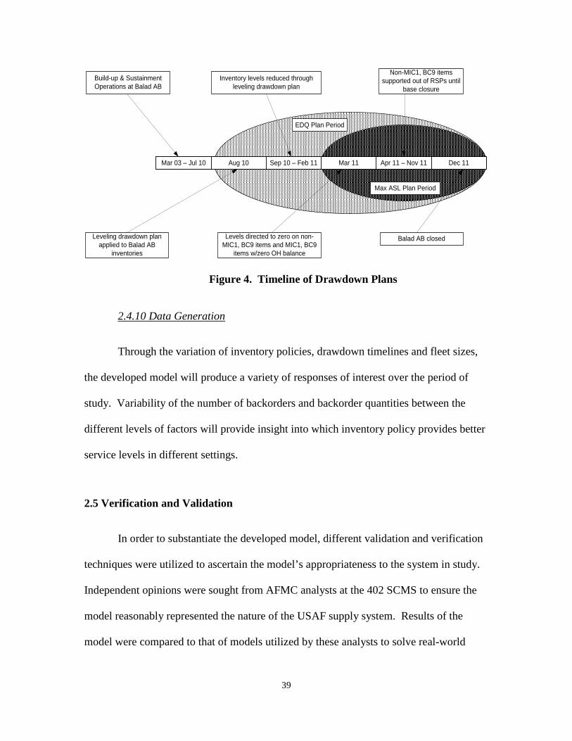
39
Mar 03 – Jul 10 Aug 10 Sep 10 – Feb 11 Mar 11 Apr 11 – Nov 11 Dec 11
EDQ Plan Period
Max ASL Plan Period
Build-up & Sustainment Operations at Balad AB
Leveling drawdown plan applied to Balad AB
inventories
Inventory levels reduced through leveling drawdown plan
Non-MIC1, BC9 items supported out of RSPs until
base closure
Levels directed to zero on non-MIC1, BC9 items and MIC1, BC9
items w/zero OH balance
Balad AB closed
Figure 4. Timeline of Drawdown Plans
Through the variation of inventory policies, drawdown timelines and fleet sizes,
the developed model will produce a variety of responses of interest over the period of
study. Variability of the number of backorders and backorder quantities between the
different levels of factors will provide insight into which inventory policy provides better
service levels in different settings.
2.4.10 Data Generation
2.5 Verification and Validation
In order to substantiate the developed model, different validation and verification
techniques were utilized to ascertain the model’s appropriateness to the system in study.
Independent opinions were sought from AFMC analysts at the 402 SCMS to ensure the
model reasonably represented the nature of the USAF supply system. Results of the
model were compared to that of models utilized by these analysts to solve real-world
40
consumable supply calculations. The feedback, suggestions and comments of these
analysts were key in making sure the coding in the model was implemented correctly.
Since the developed model simulated two inventory policies, of which one was never
enacted, the validation and verification of the model against historical data proved
impractical. Nonetheless, the output of the model’s COLT logic was compared to
outputs from spreadsheet tool used by AFMC analysts to provide a degree of validity.
2.6 Experimental Design and Methodology
The focus of this study is to measure the supply service levels over time of
different inventory reduction policies which could be utilized to support the final months
of a contingency. Based on this goal, the response variables of total number of backorder
occurrences and total quantity of backorders will be studied under different levels of the
independent factors of inventory policy and aircraft redeployment rates for three different
sizes of aircraft fleets. In this research, we only consider customer-related backorders
resulting from insufficient on-hand levels of stock, not backorders resulting from internal
supply system actions.
The factor of inventory policy is varied at two levels – one level representing the
Maximum ASL plan and the other level representing the EDQ plan. The factor of
drawdown timeline is varied at two levels - 6 and 12 months, while aircraft fleet sizes are
varied at three levels (12, 24, and 36) for 3 different experiments each with 4 treatments.
An example of the treatment levels for the fleet of 12 aircraft is presented in Table 7
below.
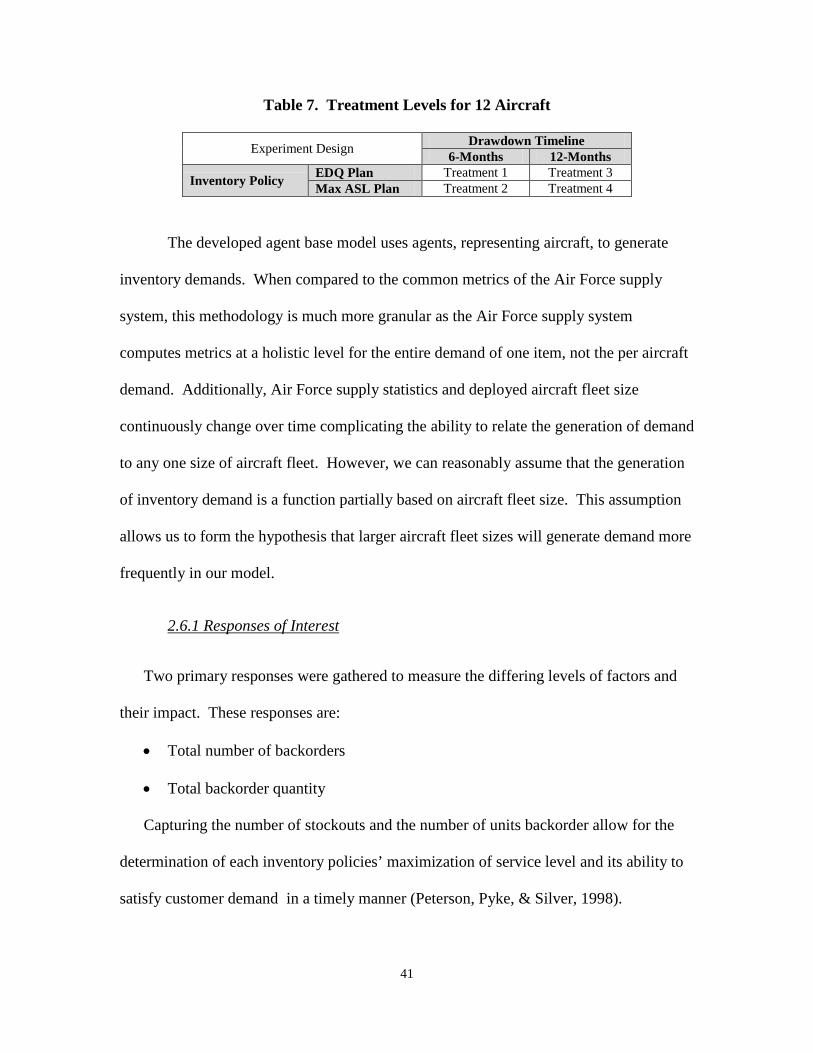
41
Table 7. Treatment Levels for 12 Aircraft
Experiment Design Drawdown Timeline 6-Months 12-Months
Inventory Policy EDQ Plan Treatment 1 Treatment 3 Max ASL Plan Treatment 2 Treatment 4
The developed agent base model uses agents, representing aircraft, to generate
inventory demands. When compared to the common metrics of the Air Force supply
system, this methodology is much more granular as the Air Force supply system
computes metrics at a holistic level for the entire demand of one item, not the per aircraft
demand. Additionally, Air Force supply statistics and deployed aircraft fleet size
continuously change over time complicating the ability to relate the generation of demand
to any one size of aircraft fleet. However, we can reasonably assume that the generation
of inventory demand is a function partially based on aircraft fleet size. This assumption
allows us to form the hypothesis that larger aircraft fleet sizes will generate demand more
frequently in our model.
Two primary responses were gathered to measure the differing levels of factors and
their impact. These responses are:
2.6.1 Responses of Interest
• Total number of backorders
• Total backorder quantity
Capturing the number of stockouts and the number of units backorder allow for the
determination of each inventory policies’ maximization of service level and its ability to
satisfy customer demand in a timely manner (Peterson, Pyke, & Silver, 1998).
42
The differentiation in the mean response values of the differing treatments for
each fleet size is analyzed with an Analysis of Variance (ANOVA) technique. The
ANOVA technique allows for the analysis and testing of the statistical significance
between the mean response values of each of the twelve treatments. Additionally, it
allows for the effects of the individual factors and the interaction between factors to be
investigated. The ANOVA techniques provide insight on how the differing inventory
policies perform for different fleet sizes redeploying at different rates. It is assumed that
the responses of interest will decrease in the treatments whose factors include an
inventory policy of EDQs and a drawdown timeline of 12 months. The ultimate goal of
using the ANOVA method is to determine if a preferred plan exists for differing fleet
sizes undergoing different drawdown rates.
2.6.2 Proposed Statistical Measures
An ANOVA for three two-factor factorial experiments will be utilized. The
validity of the ANOVA method results is predicated by the following three assumptions.
• The responses of each treatment level must be normal.
• The variance of the responses between treatment levels must be equal.
• Each treatment must be a random and independent sample.
The verification of these assumptions is required through statistical measurements to
substantiate the study’s results. The homogeneity of variances between treatment levels
is tested by the Levene’s test for equality of variances, while the normality of responses is
determined by fitting each treatment’s responses to a normal distribution curve and
testing for a goodness of fit (GoF) with the Wilk-Shapiro test statistic calculated by the
43
software package JMP. Both the test for homogeneity of variance and normality will be
conducted using a significance level of 0.05. The independence of each treatment is
assumed valid as each treatment is run independently with a unique random number
stream.
2.7 Results and Analysis
Responses for each design point were produced by conducting individual
simulations using a unique random seed generated by the default Anylogic© random
number generator. The simulation was run at each design point as an individual Monte
Carlo experiment of 31 replications to satisfy the assumptions of independence and
normality. The use of Monte Carlo experiments ensure the generation of random
numbers, while the number of replications satisfies the sample size requirements of the
Central Limit Thereom (Vogt, 2005).
The use of the ANOVA technique requires the satisficing of the three previously
mentioned assumptions. The Shapiro-Wilk goodness-of-fit test was used to evaluate to
distribution of responses for each treatment. Table 8 provides the results of each
treatment’s test as generated by the JMP software package. A p-value of less than 0.05
indicates that the test’s null hypothesis of the distribution being normal must be rejected.
2.7.1 Verification of ANOVA Assumptions

44
Table 8. Shapiro-Wilk Test Results for Responses of Interest
Treatment Total DUOs Total DUO Qty No. Inventory Policy Drawdown Timeline Fleet Size p-value p-value 1 Max ASL = 0 6 months 12 acft 0.01 0.0001 2 Max ASL = 0 6 months 24 acft 0.0005 0.0022 3 Max ASL = 0 6 months 36 acft 0.07* 0.0014 4 EDQ 6 months 12 acft 0.0001 0.0001 5 EDQ 6 months 24 acft 0.001 0.0001 6 EDQ 6 months 36 acft 0.0001 0.0001 7 Max ASL = 0 12 months 12 acft 0.0001 0.0001 8 Max ASL = 0 12 months 24 acft 0.0141 0.0001 9 Max ASL = 0 12 months 36 acft 0.0264 0.0006 10 EDQ 12 months 12 acft 0.0001 0.0001 11 EDQ 12 months 24 acft 0.0001 0.0001 12 EDQ 12 months 36 acft 0.0001 0.0001
* - Meets the assumption of normality at α=0.05
As indicated in Table 8, the assumption of normality does not hold in a majority
of the treatments. Additionally, the assumption of variance homogeneity across the
treatments must be verified. Since the proposed experiment design called for using
ANOVA to measure the difference in treatments within each fleet size, the variance of
the treatments is considered at this level. Using the Levene’ s test for equality of
variances in the JMP software package, it was determined that there was sufficient
evidence to conclude that the variances among the treatments were not equal (p-value <
0.0001). These violations of ANOVA assumptions requires the use of statistical
measures that do not rely on normality or the equality of variances.
The violations of ANOVA assumptions complicate the statistical analysis of the
developed model. These violations are probably caused by the use of discrete counts of
the response variables, rather than ensemble (moving) averages, to conduct the
2.7.2 Proposal of New Statistical Measures
45
comparisons. The preferred alternative to the proposed ANOVA technique would a non-
parametric method of multiple comparisons. A Kruskal-Wallis (K-W) test followed with
the Mann-Whitney U test for pairwise comparisons was chosen to evaluate differences
between the two inventory policies under the conditions of non-normality and unequal
variances. The K-W test is a non-parametric, or distribution free, test based on ranks of
sample observations that tests a null hypothesis for equality of population means
(Newbold, Carlson, & Thorne, 2010). As a non-parametric test, it’s only assumption is
that the sample’s observations be independent which has been previously proven. The
Mann-Whitney U Test compares two independent random samples to detect differences
in the central location of two population distributions (Newbold, Carlson, & Thorne,
2010).
A single K-W test on a categorical grouping of inventory policy and drawdown
timeline factors was conducted to evaluate differences among the policy and timeline
factors for an aircraft fleet size of 12 on median change in the number of total backorders
and total backorder quantities. The testing for the response variable of total backorders
was statistically significant with 𝑝 < 0.0001 as was the test for total backorder
quantities with 𝑝 < 0.000. These results indicate there is a statistically significant effect
on both response variables due to the changes in the inventory policy and/or the
drawdown timelines. Further testing is required to quantify specific differences.
2.7.3 Results for Fleet Size of 12
Post hoc testing was conducted using the Mann-Whitney U test with a Bonferroni
approach at a family-wise Type 1 error rate of 0.05 and individual Type 1 error rate of
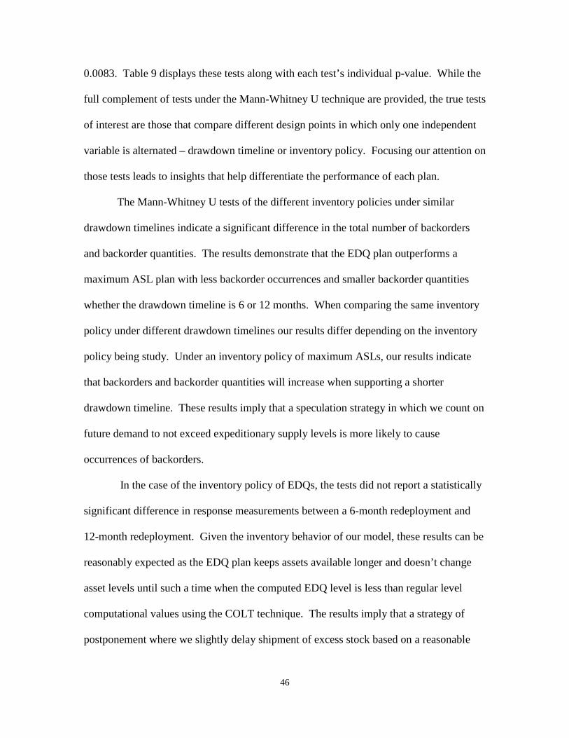
46
0.0083. Table 9 displays these tests along with each test’s individual p-value. While the
full complement of tests under the Mann-Whitney U technique are provided, the true tests
of interest are those that compare different design points in which only one independent
variable is alternated – drawdown timeline or inventory policy. Focusing our attention on
those tests leads to insights that help differentiate the performance of each plan.
The Mann-Whitney U tests of the different inventory policies under similar
drawdown timelines indicate a significant difference in the total number of backorders
and backorder quantities. The results demonstrate that the EDQ plan outperforms a
maximum ASL plan with less backorder occurrences and smaller backorder quantities
whether the drawdown timeline is 6 or 12 months. When comparing the same inventory
policy under different drawdown timelines our results differ depending on the inventory
policy being study. Under an inventory policy of maximum ASLs, our results indicate
that backorders and backorder quantities will increase when supporting a shorter
drawdown timeline. These results imply that a speculation strategy in which we count on
future demand to not exceed expeditionary supply levels is more likely to cause
occurrences of backorders.
In the case of the inventory policy of EDQs, the tests did not report a statistically
significant difference in response measurements between a 6-month redeployment and
12-month redeployment. Given the inventory behavior of our model, these results can be
reasonably expected as the EDQ plan keeps assets available longer and doesn’t change
asset levels until such a time when the computed EDQ level is less than regular level
computational values using the COLT technique. The results imply that a strategy of
postponement where we slightly delay shipment of excess stock based on a reasonable
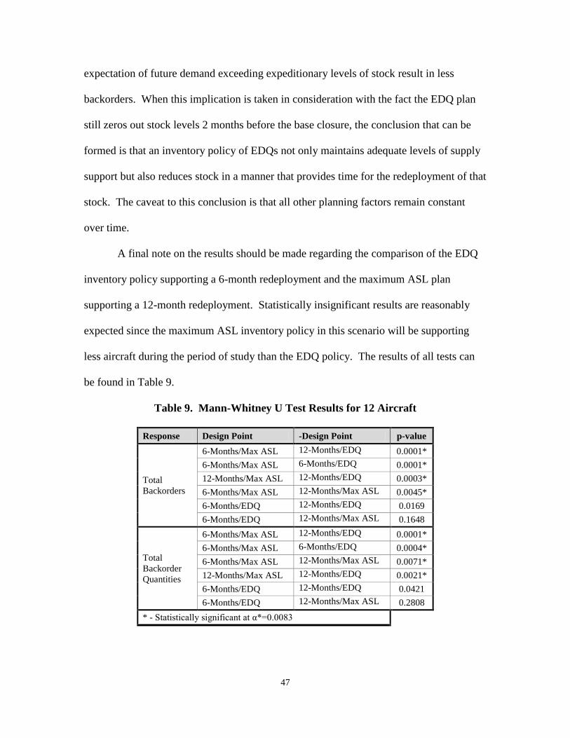
47
expectation of future demand exceeding expeditionary levels of stock result in less
backorders. When this implication is taken in consideration with the fact the EDQ plan
still zeros out stock levels 2 months before the base closure, the conclusion that can be
formed is that an inventory policy of EDQs not only maintains adequate levels of supply
support but also reduces stock in a manner that provides time for the redeployment of that
stock. The caveat to this conclusion is that all other planning factors remain constant
over time.
A final note on the results should be made regarding the comparison of the EDQ
inventory policy supporting a 6-month redeployment and the maximum ASL plan
supporting a 12-month redeployment. Statistically insignificant results are reasonably
expected since the maximum ASL inventory policy in this scenario will be supporting
less aircraft during the period of study than the EDQ policy. The results of all tests can
be found in Table 9.
Table 9. Mann-Whitney U Test Results for 12 Aircraft
Response Design Point -Design Point p-value
Total Backorders
6-Months/Max ASL 12-Months/EDQ 0.0001* 6-Months/Max ASL 6-Months/EDQ 0.0001* 12-Months/Max ASL 12-Months/EDQ 0.0003* 6-Months/Max ASL 12-Months/Max ASL 0.0045* 6-Months/EDQ 12-Months/EDQ 0.0169 6-Months/EDQ 12-Months/Max ASL 0.1648
Total Backorder Quantities
6-Months/Max ASL 12-Months/EDQ 0.0001* 6-Months/Max ASL 6-Months/EDQ 0.0004* 6-Months/Max ASL 12-Months/Max ASL 0.0071* 12-Months/Max ASL 12-Months/EDQ 0.0021* 6-Months/EDQ 12-Months/EDQ 0.0421 6-Months/EDQ 12-Months/Max ASL 0.2808
* - Statistically significant at α*=0.0083
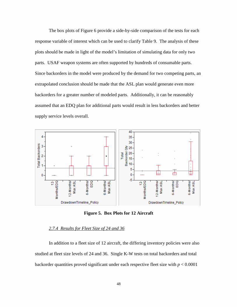
48
The box plots of Figure 6 provide a side-by-side comparison of the tests for each
response variable of interest which can be used to clarify Table 9. The analysis of these
plots should be made in light of the model’s limitation of simulating data for only two
parts. USAF weapon systems are often supported by hundreds of consumable parts.
Since backorders in the model were produced by the demand for two competing parts, an
extrapolated conclusion should be made that the ASL plan would generate even more
backorders for a greater number of modeled parts. Additionally, it can be reasonably
assumed that an EDQ plan for additional parts would result in less backorders and better
supply service levels overall.
Figure 5. Box Plots for 12 Aircraft
In addition to a fleet size of 12 aircraft, the differing inventory policies were also
studied at fleet size levels of 24 and 36. Single K-W tests on total backorders and total
backorder quantities proved significant under each respective fleet size with p < 0.0001
2.7.4 Results for Fleet Size of 24 and 36
49
for both levels of fleet sizes. Post hoc testing with a family-wise error rate of 0.05
revealed that similar results to those achieved for a fleet size of 12. The typical number
of experienced backorders and sizes of backorder quantities increase with an inventory
policy of maximum ASLs supporting a shorter drawdown timeline (6-months). These
results indicate that supply service levels, based solely on the merit of backorder
occurrences and size, increase with a linear drawdown of levels. Additionally, the results
provide insight that an EDQ plan will perform comparably over both shorter and longer
drawdown timelines. The results of the pairwise testing for each respective fleet size can
be found in Appendix S.
2.8 Conclusions
Simulation models allow for both statistical inferences and generalizations of
overall system performance. The results presented provide a generalization of how
differing inventory reduction plans would perform under representative demand trends
and differing rates of aircraft redeployments. Analysis among the different inventory
reduction policies proved statistical significant differences which lend credibility to their
relevance. The analysis, under the stated assumptions, indicates that the plan developed
by the GLSC would have created minimal backorder occurrences compared to a plan of
maximum ASLs. The developed model and subsequent analysis also indicate that
backorder occurrences in this situation are magnified under shorter redeployment
timelines. The statistical results may prove beneficial to USAF supply and senior leaders
in helping understand how to better reduce the service’s logistical footprint while
maintaining high levels of operational capability. More importantly, it is hoped that the

50
results form a foundation and provide validity towards inventory reduction policies in
future contingencies.
51
3. Case Study
Evaluation of Inventory Drawdown Policies for Balad AB
3.1 Introduction
“Our biggest challenge was getting the mission done – defending the base, providing top cover for U.S. Forces-Iraq and assisting our Iraqi hosts – while simultaneously drawing down our Airmen and equipment.”
Brigadier General Kurt Neubauer 332 Air Expeditionary Wing Commander
The year of 2011 marked significant changes in the operations of the United
States Air Force. On August 1, 2011, the United States Congress passed the Budget
Control Act of 2011, mandating $487 billion dollars in defense budgetary cuts. On
December 16, 2011 the United States Air Force (USAF) flew its final sortie over the
country of Iraq. While the budgetary cuts didn’t immediately impact operations in Iraq, it
strengthened the USAF’s resolve to maintain readiness while becoming fiscally
responsible. The quandary of maintaining the highest levels of support within tight
budgets is a constant burden under which today’s supply chains operate. It is also an
issue that the Department of Defense, and subsequently the USAF, will surely face within
the coming years as military forces are withdrawn from Afghanistan. While a majority of
the operational Air Force is still engaged in combat operations over Afghanistan, the Air
Force Logistics Management Agency (AFLMA) was tasked by the commander of the
USAF’s Global Logistics Center (GLSC) to study how well the supporting supply chain
performed in sustaining operations while decreasing inventories at the conclusion of its
mission in Iraq. Specifically, AFLMA was asked to document the process and measure
the success of the current drawdown effort at Balad Air Base AB. These lessons learned

52
would then be used for subsequent drawdown efforts. To gain a baseline for what
AFLMA was tasked to study, some background must be given on the methodologies
implemented at Balad AB to reduce its inventory before the closing of the base.
In the years 2010-2011, Balad AB underwent a transition from a contingency base
operating on sustainment stock levels to an expeditionary base operating out of RSPs
until it was ultimately transferred back to the nation of Iraq. Balad AB had been
operating with normal peacetime levels of stock, to include inventory in both a primary
operating stock (POS) and in readiness spares kits (RSPs), as studies in the past had
shown that aircraft supportability at contingency base locations improved when
additional levels of stock were applied over and above stock levels contained in RSPs
(Hunt, 2011). A plan to reduce stock over 14 months was developed by the GLSC that
aimed at gradually reducing stock levels by applying a scaling factor to an item’s daily
demand rate (DDR) (Fulk D. A., Balad Levels Drawdown Plan, 2011). The goals behind
this plan were threefold: ensure the preservation of equipment accountability, maximize
weapon system availability to the very end of operations, and support an efficient and
effective base closure effort (Fulk D. A., Balad Levels Drawdown Plan, 2011). As the
plan progressed, on hand stock and item stock levels decreased as an item’s DDR
decreased.
In early 2011, Air Force Central Command (AFCENT), with Air Staff
concurrence, issued a directive a change to the inventory drawdown plan on non-mission
capable (MIC) 1 consumable items and MIC 1 consumable items with zero on-hand
balances (Fulk D. A., Balad Levels Drawdown Plan, 2011). The directive zeroed out
stock levels in the warehouse by overriding the items’ computed stock levels with the
53
establishment of maximum adjusted stock levels (ASLs). Maximum ASLs act as a
ceiling on item stock levels by restricting stock to no more than a specified amount
(DAF, 2011). The establishment of a maximum ASL with a value of zero caused the
USAF supply system to not stock any additional quantities of the item above what was
stocked in the RSP.
Ample research exists on how to maintain inventory levels under increasing
demand over infinite time horizons. In contrast to maintaining inventory support over an
infinite horizon, a small number of studies in the past have been conducted focusing on
inventory replenishment under the conditions of decreasing demand and finite horizons.
These studies have focused on achieving optimal levels of inventory with mathematical
models on products whose market demand has diminished due to obsolescence or whose
product life cycle is fixed and experiences deterioration. Barbosa and Friedman (1979)
were a few of the first authors to explore this topic as they addressed the phasing out of
electronic products in technology markets under the assumptions of a finite time horizon
and demand function of time that eventually reaches zero. Other studies explore differing
demand trends such as exponentially declining demand (Ramani and Venkatraman, 1988;
Hill, Smith and Omar, 1998;) and linear decrease in demand (Zhao, Yang and Rand,
2000). Although very applicable to increasing our knowledge of how to address
inventory replenishment under decreasing demand, these studies can prove complicated
for decision makers. Little (2004) suggests that for a model to be of any use to a decision
maker it should be simple, robust, easy to control and adaptable to different situations.
The inventory situation experienced during Balad AB’s closure provides a unique
opportunity to investigate inventory reduction methods. It also provides an opportunity
54
to apply simulation methods as the USAF supply system is complex and alternative
designs of inventory reduction policies require analysis (Carson II, Introduction to
Modeling and Simulation, 2005). This research develops an agent-based simulation
model that can be used to study the differing inventory policies under differing factors.
Moreover, this research aims at providing a foundation for inventory reduction for future
closings of existing contingency locations.
3.3 Supply Chain Inventory Reduction Simulation
This research develops an agent-based simulation model of the sustainment
supply chain supporting Balad AB during its closure using the software AnyLogic®. The
developed simulation models inventory within both a POS and RSP source of stock.
Within the model, four inventory management processes are patterned over time
to gain an overall understanding of what factors significantly affect the topic of interest –
the manner in which the inventory of a contingency operating base should be reduced
back to expeditionary levels. The first process conceptualizes how demands are placed
on the supply chain at the air base. The second process of the model represents the
processing and fulfilling of customer demands by supporting POS and RSP inventories.
The third process abstracts the logic of inventory management computations which
underpin the management of USAF inventory. Finally, the fourth process generalizes the
resupply of inventory levels at the deployed operating base. Figure 7 provides a
graphical depiction of the four processes.
3.3.1 Model Development

55
Figure 6. Core Inventory Management Processes
To simulate demand generation at a contingency base, various demand
measurements for certain items were gathered from Balad AB’s item record through the
Logistics Installations and Mission Support-Enterprise View (LIMS-EV) as well as
historical supply transaction data obtained from the AFLMA. Rather than generalizing
demand parameters for multiple stock units, the demand factors of daily demand
frequency rate (DDFR), DDR, and variance of demand (VOD) are used as inputs to an
exponential and negative binomial distribution. The exponential distribution is used to
model demand interarrival times, while the negative binomial distribution is used to
model demand sizes.
Previous research has focused on non-MIC 1 items, but in this research focus is
given on MIC-1 items. The management of backorders in the USAF supply system
amounts to basic ABC inventory management methods in that backorders are managed in
a fashion where certain parts are given more attention than others. Those parts that
receive a majority of attention in the USAF inventory are those parts that cause aircraft to
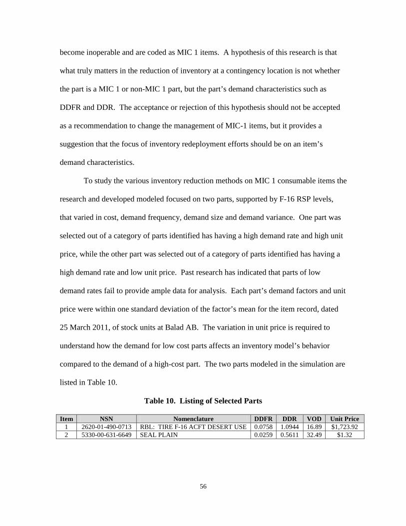
56
become inoperable and are coded as MIC 1 items. A hypothesis of this research is that
what truly matters in the reduction of inventory at a contingency location is not whether
the part is a MIC 1 or non-MIC 1 part, but the part’s demand characteristics such as
DDFR and DDR. The acceptance or rejection of this hypothesis should not be accepted
as a recommendation to change the management of MIC-1 items, but it provides a
suggestion that the focus of inventory redeployment efforts should be on an item’s
demand characteristics.
To study the various inventory reduction methods on MIC 1 consumable items the
research and developed modeled focused on two parts, supported by F-16 RSP levels,
that varied in cost, demand frequency, demand size and demand variance. One part was
selected out of a category of parts identified has having a high demand rate and high unit
price, while the other part was selected out of a category of parts identified has having a
high demand rate and low unit price. Past research has indicated that parts of low
demand rates fail to provide ample data for analysis. Each part’s demand factors and unit
price were within one standard deviation of the factor’s mean for the item record, dated
25 March 2011, of stock units at Balad AB. The variation in unit price is required to
understand how the demand for low cost parts affects an inventory model’s behavior
compared to the demand of a high-cost part. The two parts modeled in the simulation are
listed in Table 10.
Table 10. Listing of Selected Parts
Item NSN Nomenclature DDFR DDR VOD Unit Price 1 2620-01-490-0713 RBL: TIRE F-16 ACFT DESERT USE 0.0758 1.0944 16.89 $1,723.92 2 5330-00-631-6649 SEAL PLAIN 0.0259 0.5611 32.49 $1.32
57
To provide a reasonable context under which to model drawdowns of inventory at
a contingency location, the following assumptions were made:
• Data obtained through AFLMA, the GLSC, and LIMS-EV is accurate and
complete.
• Demand interarrival times are assumed to be an exponentially distributed function
of the item’s DDFR divided by a denominator equal to the average amount of
aircraft flying sorties from Balad AB on 25 Mar 2011.
• Demand size is assumed to be distributed according to the negative binomial
function with a variance calculated using the VOD formula specified by AFMAN
23-110.
• RSP demand levels are non-demand based and POS levels are demand based.
The RSP levels do not represent the actual levels of the items in RSP kits at Balad
AB, but are modeled to provide a sense of realism in the model.
• Bench stock is not modeled and assumed part of the POS inventory.
• No cannibalization, lateral resupply or local sourcing of parts. All parts are
sourced from the designated source of supply.
• No commonality exists among parts for different weapon systems.
• Delays for inbound transportation of stock are modeled at two levels, but no delay
exists for transportation of stock off base.
• RSPs are filled with any excess items from the POS inventory during the
drawdown phase of the base.
• RSPs remain at the contingency location until the end of the drawdown.
58
• No gaps in time between deployment of like MDSs at the location.
• A finite planning horizon that ends with date specified for the withdrawal of U.S.
forces from Iraq.
To substantiate a model within its domain of applicability and provide a high degree
of accuracy in its results, validation and verification of the model has to be performed
(Sargent, 2007). Since the simulation attempted to understand general inventory policy
behavior under different conditions and the policies under study had varying life spans,
validation and verification took the form of discussion with AFMC supply analysts and
output comparisons of model results to real-world analytical tools. Additionally, certain
replication outputs were compared to the stock unit’s item record to ensure that the model
reasonably produced demand at a frequency and rate comparable to the actual situation
faced at Balad AB.
3.3.2 Model Validation and Verification
Twenty-four aircraft are modeled as agents who generate demand based on a negative
binomial distribution using the inputs of an item’s DDFR, DDR, VOD and unit price.
Previous study results indicate comparable trends of supply support among varying fleet
sizes. Generation of demands for two modeled parts drive the system’s underlying
demand leveling methodologies of Economic Order Quantity (EOQ) depth or Customer
Oriented Leveling Technique (COLT) leveling. The EOQ depth model is based on
Wilson’s EOQ methods of achieving the lowest total cost in inventory, while the COLT
3.3.3 Model Execution
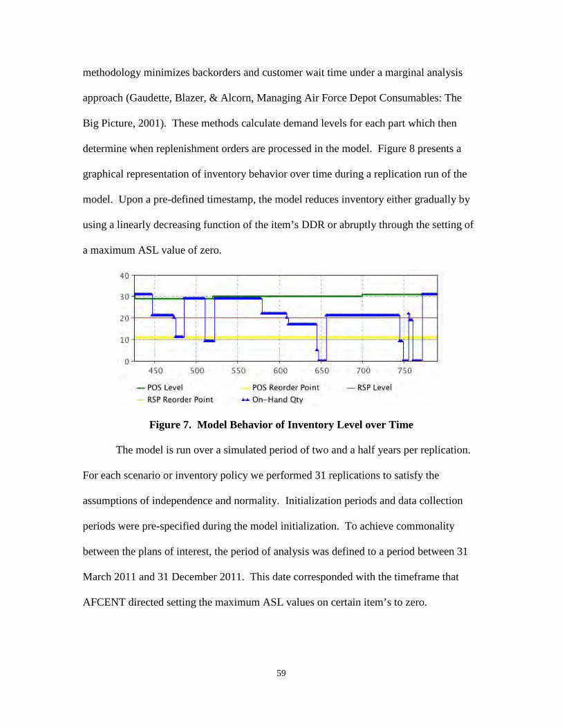
59
methodology minimizes backorders and customer wait time under a marginal analysis
approach (Gaudette, Blazer, & Alcorn, Managing Air Force Depot Consumables: The
Big Picture, 2001). These methods calculate demand levels for each part which then
determine when replenishment orders are processed in the model. Figure 8 presents a
graphical representation of inventory behavior over time during a replication run of the
model. Upon a pre-defined timestamp, the model reduces inventory either gradually by
using a linearly decreasing function of the item’s DDR or abruptly through the setting of
a maximum ASL value of zero.
Figure 7. Model Behavior of Inventory Level over Time
The model is run over a simulated period of two and a half years per replication.
For each scenario or inventory policy we performed 31 replications to satisfy the
assumptions of independence and normality. Initialization periods and data collection
periods were pre-specified during the model initialization. To achieve commonality
between the plans of interest, the period of analysis was defined to a period between 31
March 2011 and 31 December 2011. This date corresponded with the timeframe that
AFCENT directed setting the maximum ASL values on certain item’s to zero.
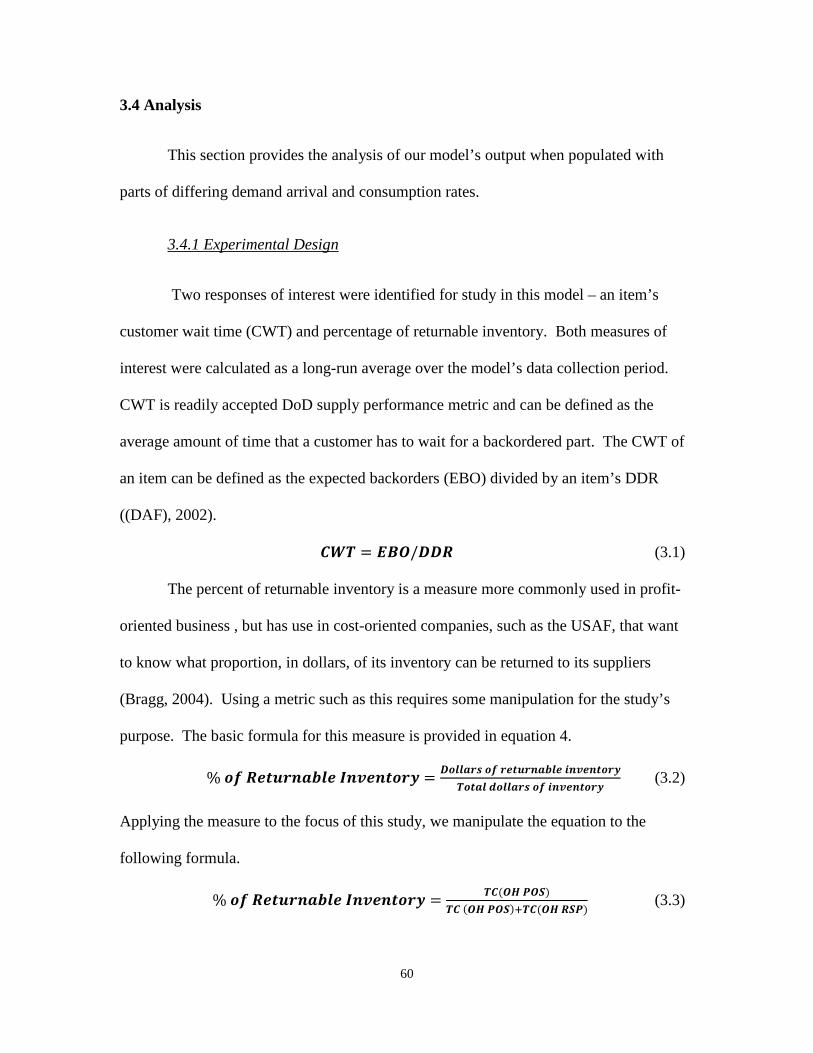
60
3.4 Analysis
This section provides the analysis of our model’s output when populated with
parts of differing demand arrival and consumption rates.
Two responses of interest were identified for study in this model – an item’s
customer wait time (CWT) and percentage of returnable inventory. Both measures of
interest were calculated as a long-run average over the model’s data collection period.
CWT is readily accepted DoD supply performance metric and can be defined as the
average amount of time that a customer has to wait for a backordered part. The CWT of
an item can be defined as the expected backorders (EBO) divided by an item’s DDR
((DAF), 2002).
3.4.1 Experimental Design
𝑪𝑾𝑻 = 𝑬𝑩𝑶/𝑫𝑫𝑹 (3.1)
The percent of returnable inventory is a measure more commonly used in profit-
oriented business , but has use in cost-oriented companies, such as the USAF, that want
to know what proportion, in dollars, of its inventory can be returned to its suppliers
(Bragg, 2004). Using a metric such as this requires some manipulation for the study’s
purpose. The basic formula for this measure is provided in equation 4.
% 𝒐𝒇 𝑹𝒆𝒕𝒖𝒓𝒏𝒂𝒃𝒍𝒆 𝑰𝒏𝒗𝒆𝒏𝒕𝒐𝒓𝒚 = 𝑫𝒐𝒍𝒍𝒂𝒓𝒔 𝒐𝒇 𝒓𝒆𝒕𝒖𝒓𝒏𝒂𝒃𝒍𝒆 𝒊𝒏𝒗𝒆𝒏𝒕𝒐𝒓𝒚𝑻𝒐𝒕𝒂𝒍 𝒅𝒐𝒍𝒍𝒂𝒓𝒔 𝒐𝒇 𝒊𝒏𝒗𝒆𝒏𝒕𝒐𝒓𝒚
(3.2)
Applying the measure to the focus of this study, we manipulate the equation to the
following formula.
% 𝒐𝒇 𝑹𝒆𝒕𝒖𝒓𝒏𝒂𝒃𝒍𝒆 𝑰𝒏𝒗𝒆𝒏𝒕𝒐𝒓𝒚 = 𝑻𝑪(𝑶𝑯 𝑷𝑶𝑺)𝑻𝑪 (𝑶𝑯 𝑷𝑶𝑺)+𝑻𝑪(𝑶𝑯 𝑹𝑺𝑷)
(3.3)

61
where TC(OH POS) is the total cost of on-hand stock in the primary operating stock and
TC(OH RSP) is the total cost of on-hand stock in the RSP. The total cost of on-hand
stock is defined as the unit price of each item plus its holding cost and ordering cost.
The measures of interest were analyzed under the effect of different inventory
policies and aircraft redeployment timeline and rates. Inventory policy factors include
ordinal factors that identify the two plans used at Balad AB – setting a maximum ASL
value to zero or the reduction of stock as a linear function of the item’s DDR. Aircraft
redeployment timelines were the ordinal factors of 6 and 12 months. It is during this
timeline that the 24-ship fleet would be deleted from the model in whole integers (4 ships
per month for a 6 month redeployment and 2 ships per month for a 12 month
redeployment). CWT analysis is provided in the form of a full-factorial 22 experiment
while the percentage of returnable inventory analysis, due to violations of normality and
equal variances, was conducted using the non-parametric Kurskal-Wallis (K-W) test with
post-hoc analysis generated by the Mann-Whitney U test.
Responses for each treatment level were based on the outputs of individual Monte
Carlo experiments run over 31 replications. The use of Monte Carlo experiments ensured
the generation of independent samples, while the number of replications satisfies the
sample size requirements of the Central Limit Theorem (Vogt, 2005). Each replication
was run for 2 and 1/2 years of simulated operations time with the first 21 months of data
deleted. The lengthy initialization period is required to stabilize the long-run average
calculations of the simulated USAF supply system. A data collection period of 9 months
3.4.2 Results
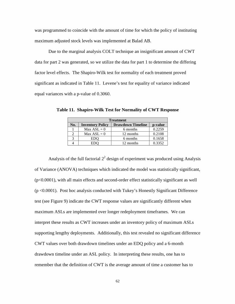
62
was programmed to coincide with the amount of time for which the policy of instituting
maximum adjusted stock levels was implemented at Balad AB.
Due to the marginal analysis COLT technique an insignificant amount of CWT
data for part 2 was generated, so we utilize the data for part 1 to determine the differing
factor level effects. The Shapiro-Wilk test for normality of each treatment proved
significant as indicated in Table 11. Levene’s test for equality of variance indicated
equal variances with a p-value of 0.3060.
Table 11. Shapiro-Wilk Test for Normality of CWT Response
Treatment No. Inventory Policy Drawdown Timeline p-value 1 Max ASL = 0 6 months 0.2259 2 Max ASL = 0 12 months 0.2108 3 EDQ 6 months 0.1658 4 EDQ 12 months 0.3352
Analysis of the full factorial 22 design of experiment was produced using Analysis
of Variance (ANOVA) techniques which indicated the model was statistically significant,
(p<0.0001), with all main effects and second-order effect statistically significant as well
(p <0.0001). Post hoc analysis conducted with Tukey’s Honestly Significant Difference
test (see Figure 9) indicate the CWT response values are significantly different when
maximum ASLs are implemented over longer redeployment timeframes. We can
interpret these results as CWT increases under an inventory policy of maximum ASLs
supporting lengthy deployments. Additionally, this test revealed no significant difference
CWT values over both drawdown timelines under an EDQ policy and a 6-month
drawdown timeline under an ASL policy. In interpreting these results, one has to
remember that the definition of CWT is the average amount of time a customer has to
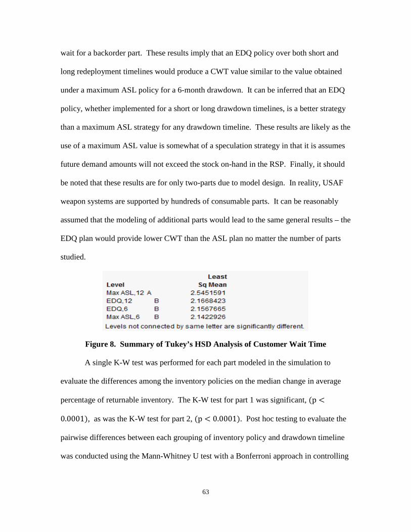
63
wait for a backorder part. These results imply that an EDQ policy over both short and
long redeployment timelines would produce a CWT value similar to the value obtained
under a maximum ASL policy for a 6-month drawdown. It can be inferred that an EDQ
policy, whether implemented for a short or long drawdown timelines, is a better strategy
than a maximum ASL strategy for any drawdown timeline. These results are likely as the
use of a maximum ASL value is somewhat of a speculation strategy in that it is assumes
future demand amounts will not exceed the stock on-hand in the RSP. Finally, it should
be noted that these results are for only two-parts due to model design. In reality, USAF
weapon systems are supported by hundreds of consumable parts. It can be reasonably
assumed that the modeling of additional parts would lead to the same general results – the
EDQ plan would provide lower CWT than the ASL plan no matter the number of parts
studied.
Figure 8. Summary of Tukey’s HSD Analysis of Customer Wait Time
A single K-W test was performed for each part modeled in the simulation to
evaluate the differences among the inventory policies on the median change in average
percentage of returnable inventory. The K-W test for part 1 was significant, (p <
0.0001), as was the K-W test for part 2, (p < 0.0001). Post hoc testing to evaluate the
pairwise differences between each grouping of inventory policy and drawdown timeline
was conducted using the Mann-Whitney U test with a Bonferroni approach in controlling
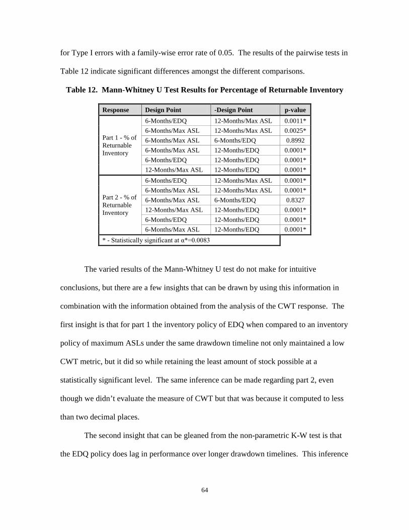
64
for Type I errors with a family-wise error rate of 0.05. The results of the pairwise tests in
Table 12 indicate significant differences amongst the different comparisons.
Table 12. Mann-Whitney U Test Results for Percentage of Returnable Inventory
Response Design Point -Design Point p-value
Part 1 - % of Returnable Inventory
6-Months/EDQ 12-Months/Max ASL 0.0011* 6-Months/Max ASL 12-Months/Max ASL 0.0025* 6-Months/Max ASL 6-Months/EDQ 0.8992 6-Months/Max ASL 12-Months/EDQ 0.0001* 6-Months/EDQ 12-Months/EDQ 0.0001* 12-Months/Max ASL 12-Months/EDQ 0.0001*
Part 2 - % of Returnable Inventory
6-Months/EDQ 12-Months/Max ASL 0.0001* 6-Months/Max ASL 12-Months/Max ASL 0.0001* 6-Months/Max ASL 6-Months/EDQ 0.8327 12-Months/Max ASL 12-Months/EDQ 0.0001* 6-Months/EDQ 12-Months/EDQ 0.0001* 6-Months/Max ASL 12-Months/EDQ 0.0001*
* - Statistically significant at α*=0.0083
The varied results of the Mann-Whitney U test do not make for intuitive
conclusions, but there are a few insights that can be drawn by using this information in
combination with the information obtained from the analysis of the CWT response. The
first insight is that for part 1 the inventory policy of EDQ when compared to an inventory
policy of maximum ASLs under the same drawdown timeline not only maintained a low
CWT metric, but it did so while retaining the least amount of stock possible at a
statistically significant level. The same inference can be made regarding part 2, even
though we didn’t evaluate the measure of CWT but that was because it computed to less
than two decimal places.
The second insight that can be gleaned from the non-parametric K-W test is that
the EDQ policy does lag in performance over longer drawdown timelines. This inference
65
can be made when viewing the results of those tests that compare the EDQ inventory
policy over different drawdown timelines. This result is consistent with the logic
programmed in the model since the EDQ plan is a function of an item’s DDR which is
equivalent to an 18-month moving average. The EDQ plan supporting a 12-month
drawdown would not begin to bring levels down until the final months of the drawdown
as indicated by the higher mean in the K-W test. A feasible suggestion regarding this
insight is to compute an item’s DDR over a smaller window as the contingency’s
conclusion becomes more imminent. This suggestion, though, has to be weighed with the
costs associated with managing such a plan under changing conditions.
3.5 Conclusions
This model and analysis explored the impacts of the differing inventory policies
supporting various redeployment rates of supported aircraft. Two inventory policies were
studied – setting of a maximum adjusted stock level to a value of zero or the linear
reduction of stock as a function of an item’s DDR. The intent of this study was to gain
further insight on which plan may better support the closure of contingency base while
maintaining adequate levels of supply support to the warfighter. The results provided
significant differences and insights between the two plans. The further examination of
these two plans will aid in a conclusive strategy for future contingency base closures.
66
4. Conclusion
4.1 Introduction
This chapter provides a summary of the research performed during the course of
examining the performance of different inventory policies supporting different fleet sizes
undergoing varying rates of redeployment. The chapter begins with a general overview
of the thesis, followed by the findings and conclusions derived from the analysis of our
simulation model’s output data. The chapter concludes by providing a list of topics
encountered during the course of this research that would be suitable for future study.
4.2 Research Summary
This focus of this study was to develop an agent-based simulation to evaluate
different inventory reduction plans that could be used to decrease inventory at bases
operating in a contingency location. The fundamental inventory management processes
of USAF consumables were programmed and historical data was used to generate
stochastic demands. Constraining assumptions were made to bind the model and
programming logic in a fashion suitable for analysis. While agent-based modeling has
been available for use during the past two decades, this model provides a novel approach
and a broader understanding of factors affecting supply support in wartime environments
not previously researched.
Furthermore, an additional examination was provided on how support to MIC 1
coded items could be affected with various inventory reduction plans. This analysis was
67
conducted using customer wait time as a measurement. As this research addresses only a
few approaches to studying supply support at contingency locations, many other
approaches and factors should be studied to ascertain a higher degree of fidelity on
different supply support plans and inventory management policies for future contingency
base closures.
4.3 Summary of Findings
In this section, the basic research questions posed in Chapter 1 will be addressed
based on the analysis of data provided in Chapters 2 and 3. The questions from Chapter 1
are:
1. Should drawdowns, at the system level, of inventory at contingency locations be treated any differently than the redistribution of excess inventory at peacetime locations? This question simply asks if basing an inventory drawdown plan off of an item or
group of item’s DDR is better suited to drawing down assets and asset levels versus using
the MCDDR technique described in AFMAN 23-110, Volume 2, Part 2, Chapter 19.
There exists an inherit difference between the plan developed by GLSC and the formula
for MCDDRs and MCDDFRs – the use of sortie information. While the developed
model did not explicitly utilize sortie information as an input or output parameter, the
long-run behavior of each replication did provide some insight into the reduction of stock
as a function of the DDR. Long-run behavior indicated that reducing stock as a function
of the DDR suffers from performance lags when the basic DDR formula from AFMAN
23-110 is utilized. Since the basic formula is an essentially an 18-month moving average
this behavior should be expected. In contrast, using the DDR to drive the decrease of
68
inventory levels creates a flexible plan that not only reduces stock but also maintains high
customer support levels. This point was alluded to by the GLSC when their plan for the
Balad AB closure was developed (Fulk D. A., Balad Levels Drawdown Plan, 2011).
Further testing is required to determine if the reduction of stock as a function of the DDR
would perform any better than using the basic MCDDR and MCDDFR formulas in
AFMAN 23-110.
2. Is there a statistical and/or practical difference among policies for reducing inventory levels in the final phases of a contingency operation? The results of Chapter 2 and 3 indicate that there is a statistical difference
between the two policies enacted at Balad AB. According to statistical tests, the use of
maximum ASLs is more likely to increase the median and mean number of backorders
and backorder quantities. Also, these tests indicate that the plan developed by the GLSC
would minimize total backorders and backorder amounts over both 6-month and 12-
month redeployment timelines. The model’s behavior indicates a practical significance
among the differing policies in that use of maximum ASL, no matter the type of item, is
somewhat of a speculation strategy in that we expect future demands to be no more than
on-hand asset quantities contained within the RSPs. According to the model’s behavior
and output, this strategy is found lacking in support to aircraft fleets undergoing shorter
redeployments.
3. What are appropriate measures to be used in evaluating policies for drawdown of inventory in a contingency environment? The results of the study indicate that the answer to this question is a mix of
metrics. The use of CWT throughout the redeployment is still a requirement as

69
operations may have to be maintained up until the final day. The study has found that a
formula based on unused inventory remaining may provide a leading indicator of how
well the USAF is achieving its objective of closing the base down in a reasonable
fashion. These are only two metrics and their use should be in conjunction with other
supply metrics to form a better picture of the drawdown effort.
4. What parameters should guide inventory drawdowns in future contingency operations?
This study focused on four parameters – DDFR, DDR, VOD, and unit price. Of
the four, an item’s DDR, VOD and unit price affected inventory behavior the most. DDR
and VOD accounted for the variation in demand sizes generated by the model. Items
with low DDRs and VODs failed to produce any substantial results for this study, while
items with higher DDRs and VODs produced more backorders. Also of interesting note
was that items with lower unit prices performed reasonably better than those with higher
unit prices. This behavior should have been expected as the marginal analysis
methodology used in COLT would rather prevent backorders for a cheaper part than an
expensive part, but the extent to which unit price played a factor was somewhat
astounding. Unit price was the driving factor in the model failing to produce CWT
values for low cost items. In future contingencies, the use of an item’s DDR, VOD and
unit price should be taken into consideration as these three parameters exhibited the
tendency to affect the model’s performance the most.

70
4.4 Future Work
The developed model has been programmed in such a manner that it provides
flexibility for future studies. The number of parameters available for modification
provides opportunities for future studies to explore the impacts of various factors such as
transportation, up-stream supplier stock availability and pertinent pecuniary costs that
affect supply decisions. The capabilities that have already been programmed thus
decrease the time required to adapt the model to other studies. As this model addresses
only a certain type of part – consumables – there are additional areas of expansions that
should be considered. We suggest the following topics:
• The modeling of sorties within the aircraft agent and the subsequent capture of
sorties information generated by the agent.
• The implementation of MCDDR and MCDDFRs based on sortie information.
• The modeling of maintenance information to provide a more realistic picture of
demand interarrival time.
• The parameterization of differing RSP and DLA support levels within the model
could allow for a more representative picture of a contingency supply chain.
• The modeling or more than two parts within the model. The marginal analysis
technique performed by the COLT methodology compares a multitude of parts to
derive levels of stock that minimize the over number of backorders and customer
wait time.
• The modification of the model to include better time-based averages such as
average number of daily backorders.
71
Substantial opportunities exist for the expansion of this study and future
operations may necessitate an extension of a similar model. The limitations in this model
are solely of the author’s doing, not the methodology or software. Few academic studies
exist that explore inventory replenishment under decreasing demand with even fewer
studies evaluating this topic utilizing agent-based modeling. Additionally, the use of
agent-based models in military research has still not matured to a level of common use.
It is hoped that this simulation model and the subsequent analysis has provided insight
into future inventory reduction plans and the applicability of an agent-based modeling
simulation approach to understanding problems facing the Air Force.
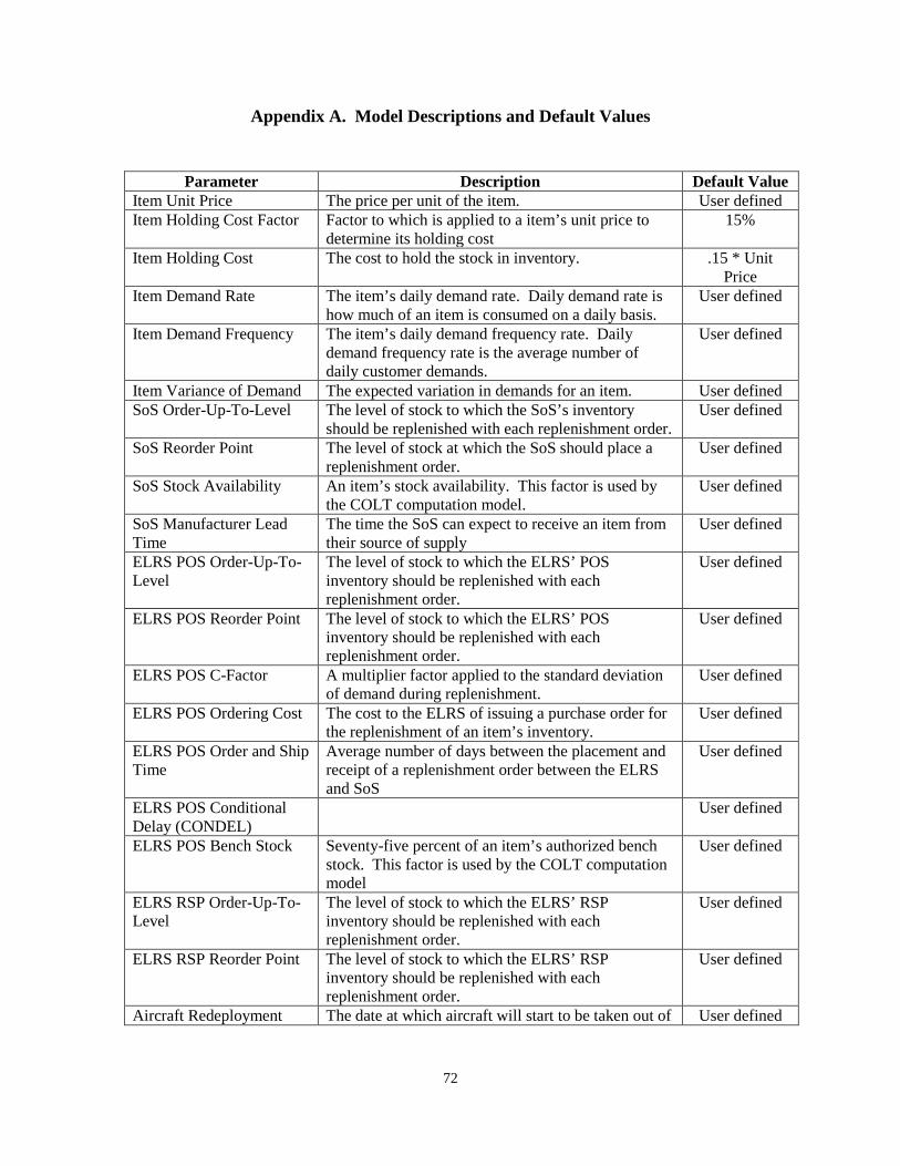
72
Appendix A. Model Descriptions and Default Values
Parameter Description Default Value
Item Unit Price The price per unit of the item. User defined Item Holding Cost Factor Factor to which is applied to a item’s unit price to
determine its holding cost 15%
Item Holding Cost The cost to hold the stock in inventory. .15 * Unit Price
Item Demand Rate The item’s daily demand rate. Daily demand rate is how much of an item is consumed on a daily basis.
User defined
Item Demand Frequency The item’s daily demand frequency rate. Daily demand frequency rate is the average number of daily customer demands.
User defined
Item Variance of Demand The expected variation in demands for an item. User defined SoS Order-Up-To-Level The level of stock to which the SoS’s inventory
should be replenished with each replenishment order. User defined
SoS Reorder Point The level of stock at which the SoS should place a replenishment order.
User defined
SoS Stock Availability An item’s stock availability. This factor is used by the COLT computation model.
User defined
SoS Manufacturer Lead Time
The time the SoS can expect to receive an item from their source of supply
User defined
ELRS POS Order-Up-To-Level
The level of stock to which the ELRS’ POS inventory should be replenished with each replenishment order.
User defined
ELRS POS Reorder Point The level of stock to which the ELRS’ POS inventory should be replenished with each replenishment order.
User defined
ELRS POS C-Factor A multiplier factor applied to the standard deviation of demand during replenishment.
User defined
ELRS POS Ordering Cost The cost to the ELRS of issuing a purchase order for the replenishment of an item’s inventory.
User defined
ELRS POS Order and Ship Time
Average number of days between the placement and receipt of a replenishment order between the ELRS and SoS
User defined
ELRS POS Conditional Delay (CONDEL)
User defined
ELRS POS Bench Stock Seventy-five percent of an item’s authorized bench stock. This factor is used by the COLT computation model
User defined
ELRS RSP Order-Up-To-Level
The level of stock to which the ELRS’ RSP inventory should be replenished with each replenishment order.
User defined
ELRS RSP Reorder Point The level of stock to which the ELRS’ RSP inventory should be replenished with each replenishment order.
User defined
Aircraft Redeployment The date at which aircraft will start to be taken out of User defined
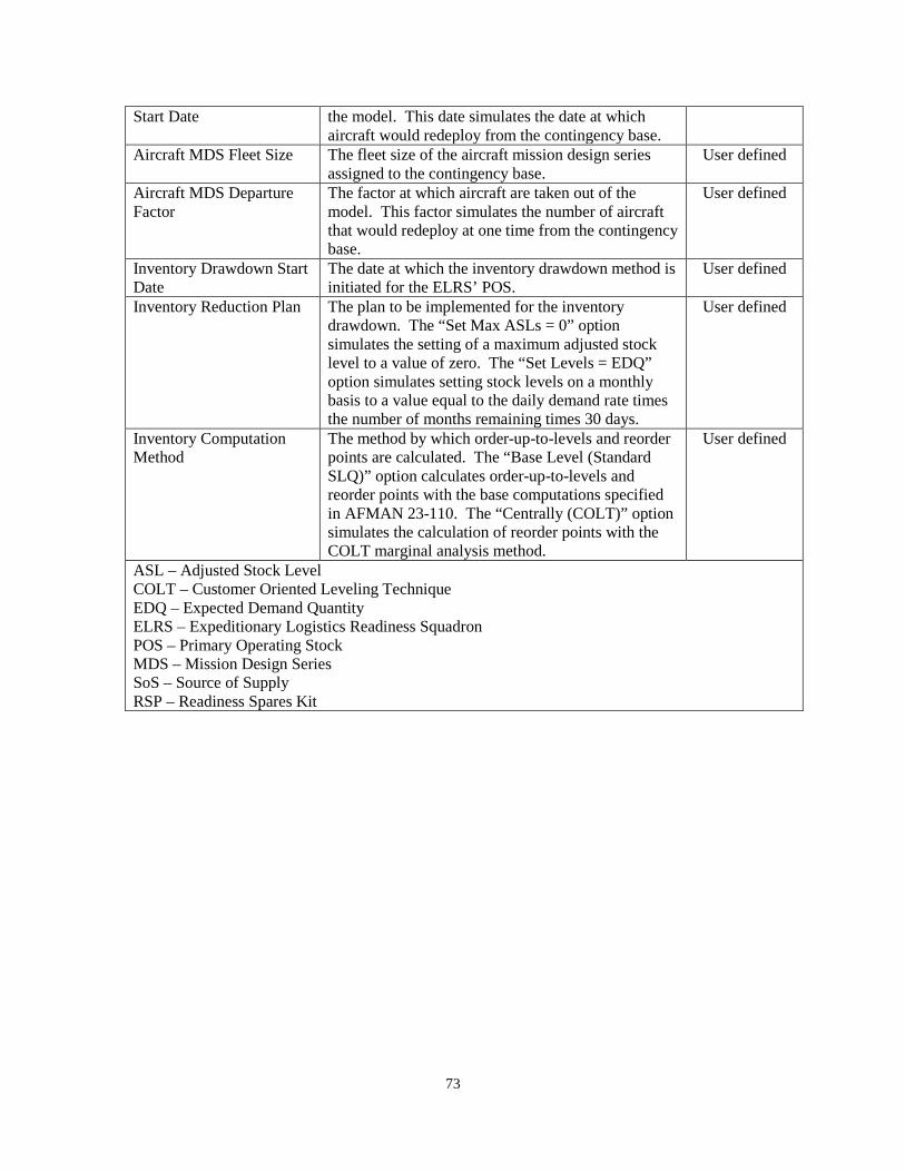
73
Start Date the model. This date simulates the date at which aircraft would redeploy from the contingency base.
Aircraft MDS Fleet Size The fleet size of the aircraft mission design series assigned to the contingency base.
User defined
Aircraft MDS Departure Factor
The factor at which aircraft are taken out of the model. This factor simulates the number of aircraft that would redeploy at one time from the contingency base.
User defined
Inventory Drawdown Start Date
The date at which the inventory drawdown method is initiated for the ELRS’ POS.
User defined
Inventory Reduction Plan The plan to be implemented for the inventory drawdown. The “Set Max ASLs = 0” option simulates the setting of a maximum adjusted stock level to a value of zero. The “Set Levels = EDQ” option simulates setting stock levels on a monthly basis to a value equal to the daily demand rate times the number of months remaining times 30 days.
User defined
Inventory Computation Method
The method by which order-up-to-levels and reorder points are calculated. The “Base Level (Standard SLQ)” option calculates order-up-to-levels and reorder points with the base computations specified in AFMAN 23-110. The “Centrally (COLT)” option simulates the calculation of reorder points with the COLT marginal analysis method.
User defined
ASL – Adjusted Stock Level COLT – Customer Oriented Leveling Technique EDQ – Expected Demand Quantity ELRS – Expeditionary Logistics Readiness Squadron POS – Primary Operating Stock MDS – Mission Design Series SoS – Source of Supply RSP – Readiness Spares Kit
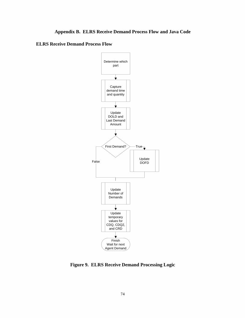
74
Appendix B. ELRS Receive Demand Process Flow and Java Code
ELRS Receive Demand Process Flow
Capture demand time and quantity
Update DOLD and
Last Demand Amount
First Demand?
Update DOFD
Update Number of Demands
Update temporary values for
CDQ, CDQ2, and CRD
True
False
FinishWait for next
Agent Demand
Determine which part
Figure 9. ELRS Receive Demand Processing Logic
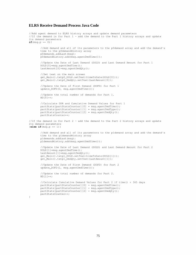
75
ELRS Receive Demand Process Java Code //Add agent demand to ELRS history arrays and update demand parameters //If the demand is for Part 1 - add the demand to the Part 1 history arrays and update its demand parameters if(msg.p == 0){
//Add demand and all of its parameters to the p0demand array and add the demand's time to the p0demandHistory array
p0demands.addLast(msg); p0demandHistory.add(msg.agentDmdTime());
//Update the Date of Last Demand (DOLD) and Last Demand Amount for Part 1 DOLD[0]=msg.agentDmdTime(); LastAmount[0]=msg.agentDmdQty(); //Set text on the main screen get_Main().txtp0_DOLD.setText(timeToDate(DOLD[0])); get_Main().txtp0_DmdQty.setText(LastAmount[0]); //Update the Date of First Demand (DOFD) for Part 1 update_DOFD(0, msg.agentDmdTime()); //Update the total number of demands for Part 1. ND[0]++; //Calculate DDR and Cumulative Demand Values for Part 1 partStats[partStatsCounter][0] = msg.agentDmdTime(); partStats[partStatsCounter][1] = msg.agentDmdType(); partStats[partStatsCounter][2] = msg.agentDmdQty(); partStatsCounter++; //If the demand is for Part 2 - add the demand to the Part 2 history arrays and update its demand parameters }else if(msg.p == 1){
//Add demand and all of its parameters to the p1demand array and add the demand's time to the p1demandHistory array
p1demands.addLast(msg); p1demandHistory.add(msg.agentDmdTime());
//Update the Date of Last Demand (DOLD) and Last Demand Amount for Part 2 DOLD[1]=msg.agentDmdTime(); LastAmount[1]=msg.agentDmdQty(); get_Main().txtp1_DOLD.setText(timeToDate(DOLD[1])); get_Main().txtp1_DmdQty.setText(LastAmount[1]); //Update the Date of First Demand (DOFD) for Part 2 update_DOFD(1, msg.agentDmdTime()); //Update the total number of demands for Part 2. ND[1]++;
//Calculate Cumulative Demand Values for Part 2 if time() < 365 days partStats[partStatsCounter][0] = msg.agentDmdTime(); partStats[partStatsCounter][1] = msg.agentDmdType(); partStats[partStatsCounter][2] = msg.agentDmdQty(); partStatsCounter++; }
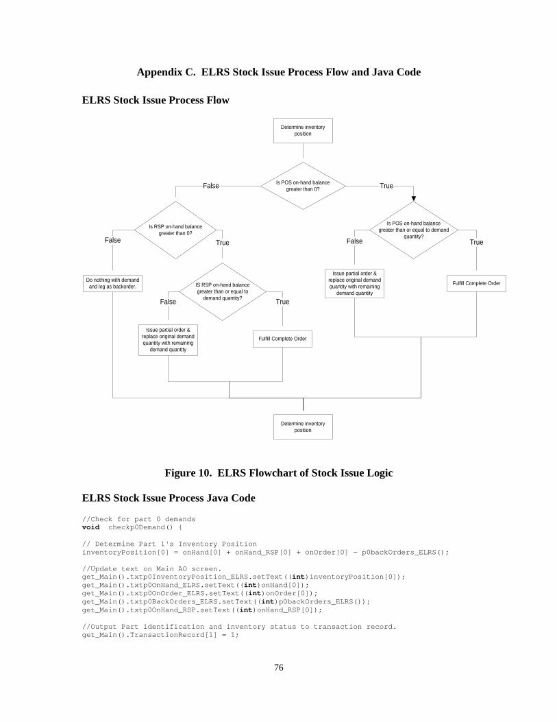
76
Appendix C. ELRS Stock Issue Process Flow and Java Code
ELRS Stock Issue Process Flow
Determine inventory position
Is POS on-hand balance greater than 0?
Is POS on-hand balance greater than or equal to demand
quantity?
Fulfill Complete Order
Issue partial order & replace original demand quantity with remaining
demand quantity
Is RSP on-hand balance greater than 0?
IS RSP on-hand balance greater than or equal to
demand quantity?
Do nothing with demand and log as backorder.
Fulfill Complete OrderIssue partial order &
replace original demand quantity with remaining
demand quantity
Determine inventory position
TrueFalse
False TrueTrueFalse
False True
Figure 10. ELRS Flowchart of Stock Issue Logic
ELRS Stock Issue Process Java Code
//Check for part 0 demands void checkp0Demand() { // Determine Part 1's Inventory Position inventoryPosition[0] = onHand[0] + onHand_RSP[0] + onOrder[0] - p0backOrders_ELRS(); //Update text on Main AO screen. get_Main().txtp0InventoryPosition_ELRS.setText((int)inventoryPosition[0]); get_Main().txtp0OnHand_ELRS.setText((int)onHand[0]); get_Main().txtp0OnOrder_ELRS.setText((int)onOrder[0]); get_Main().txtp0BackOrders_ELRS.setText((int)p0backOrders_ELRS()); get_Main().txtp0OnHand_RSP.setText((int)onHand_RSP[0]); //Output Part identification and inventory status to transaction record. get_Main().TransactionRecord[1] = 1;
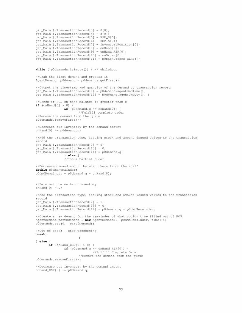
77
get_Main().TransactionRecord[3] = S[0]; get_Main().TransactionRecord[4] = s[0]; get_Main().TransactionRecord[5] = RSP_S[0]; get_Main().TransactionRecord[6] = RSP_s[0]; get_Main().TransactionRecord[7] = inventoryPosition[0]; get_Main().TransactionRecord[8] = onHand[0]; get_Main().TransactionRecord[9] = onHand_RSP[0]; get_Main().TransactionRecord[10] = onOrder[0]; get_Main().TransactionRecord[11] = p0backOrders_ELRS(); while (!p0demands.isEmpty()) { // whileLoop //Grab the first demand and process it AgentDemand p0demand = p0demands.getFirst(); //Output the timestamp and quantity of the demand to transaction record get_Main().TransactionRecord[0] = p0demand.agentDmdTime(); get_Main().TransactionRecord[12] = p0demand.agentDmdQty(); ; //Check if POS on-hand balance is greater than 0 if (onHand[0] > 0) { if (p0demand.q <= onHand[0]) { //Fulfill complete order //Remove the demand from the queue p0demands.removeFirst(); //Decrease our inventory by the demand amount onHand[0] -= p0demand.q; //Add the transaction type, issuing stock and amount issued values to the transaction record get_Main().TransactionRecord[2] = 0; get_Main().TransactionRecord[13] = 0; get_Main().TransactionRecord[14] = p0demand.q; } else { //Issue Partial Order //Decrease demand amount by what there is on the shelf double p0dmdRemainder; p0dmdRemainder = p0demand.q - onHand[0]; //Zero out the on-hand inventory onHand[0] = 0; //Add the transaction type, issuing stock and amount issued values to the transaction record get_Main().TransactionRecord[2] = 1; get_Main().TransactionRecord[13] = 0; get_Main().TransactionRecord[14] = p0demand.q - p0dmdRemainder; //Create a new demand for the remainder of what couldn't be filled out of POS AgentDemand part0Demand = new AgentDemand(0, p0dmdRemainder, time()); p0demands.set(0, part0Demand); //Out of stock - stop processing break; } } else { if (onHand_RSP[0] > 0) { if (p0demand.q <= onHand_RSP[0]) { //Fulfill Complete Order //Remove the demand from the queue p0demands.removeFirst(); //Decrease our inventory by the demand amount onHand_RSP[0] -= p0demand.q;

78
//Add the transaction type, issuing stock and amount issued values to the transaction record get_Main().TransactionRecord[2] = 0; get_Main().TransactionRecord[13] = 1; get_Main().TransactionRecord[14] = p0demand.q; } else { //Issue Partial Order //Decrease demand amount by what there is on the shelf double p0dmdRemainder2; p0dmdRemainder2 = p0demand.q - onHand_RSP[0]; AgentDemand part0Demand2 = new AgentDemand(0, p0dmdRemainder2, time()); p0demands.set(0, part0Demand2); //Zero out the on-hand RSP inventory onHand_RSP[0] = 0; //Add the transaction type, issuing stock and amount issued values to the transaction record get_Main().TransactionRecord[2] = 1; get_Main().TransactionRecord[13] = 1; get_Main().TransactionRecord[14] = p0demand.q - p0dmdRemainder2; //Out of stock - stop-processing. break; } } else { //Tally BOs //Increase the count of backorders for this part ieBOs[0]++; //Add the transaction type, issuing stock and amount issued values to the transaction record get_Main().TransactionRecord[2] = 2; get_Main().TransactionRecord[13] = 99; get_Main().TransactionRecord[14] = 0; //Out of stock - stop processing break; } } // UpdateVisualControls if(onHand[0] > 0){ p0onHand_Replicator = onHand[0]; }else if(onHand[0] <= 0){ p0onHand_Replicator = 0; } if(onHand_RSP[0] > 0){ p0RSPOH_Replicator = onHand_RSP[0]; }else if(onHand[0] <= 0){ p0RSPOH_Replicator = 0; } } // whileLoop // Determine Part 1's Inventory Position inventoryPosition[0] = onHand[0] + onHand_RSP[0] + onOrder[0] - p0backOrders_ELRS(); //Update text on main screen get_Main().txtp0InventoryPosition_ELRS.setText((int)inventoryPosition[0]); get_Main().txtp0OnHand_ELRS.setText((int)onHand[0]); get_Main().txtp0OnOrder_ELRS.setText((int)onOrder[0]); get_Main().txtp0BackOrders_ELRS.setText((int)p0backOrders_ELRS()); get_Main().txtp0OnHand_RSP.setText((int)onHand_RSP[0]);
79
//Set order amount value and time to default values since this isn’t a replenishment order get_Main().TransactionRecord[15] = 9999; get_Main().TransactionRecord[16] = 9999; get_Main().TransactionRecord[17] = 9999; get_Main().TransactionRecord[18] = 9999; get_Main().TransactionRecord[19] = 9999; get_Main().TransactionRecord[20] = 9999; String transaction = ""; transaction = format(timeToDate(get_Main().TransactionRecord[0])); //Capture data on date specified by user if(time() >= Simulation_MC.CaptureDataStart){ for(int a = 1; a<= 20; a++){ transaction += "\\" + get_Main().TransactionRecord[a]; } Collections.addAll(Simulation_MC.TransactionHistory, transaction); } for(int j = 0; j <= 20; j++){ get_Main().TransactionRecord[j] = 0; } transaction = ""; return; }
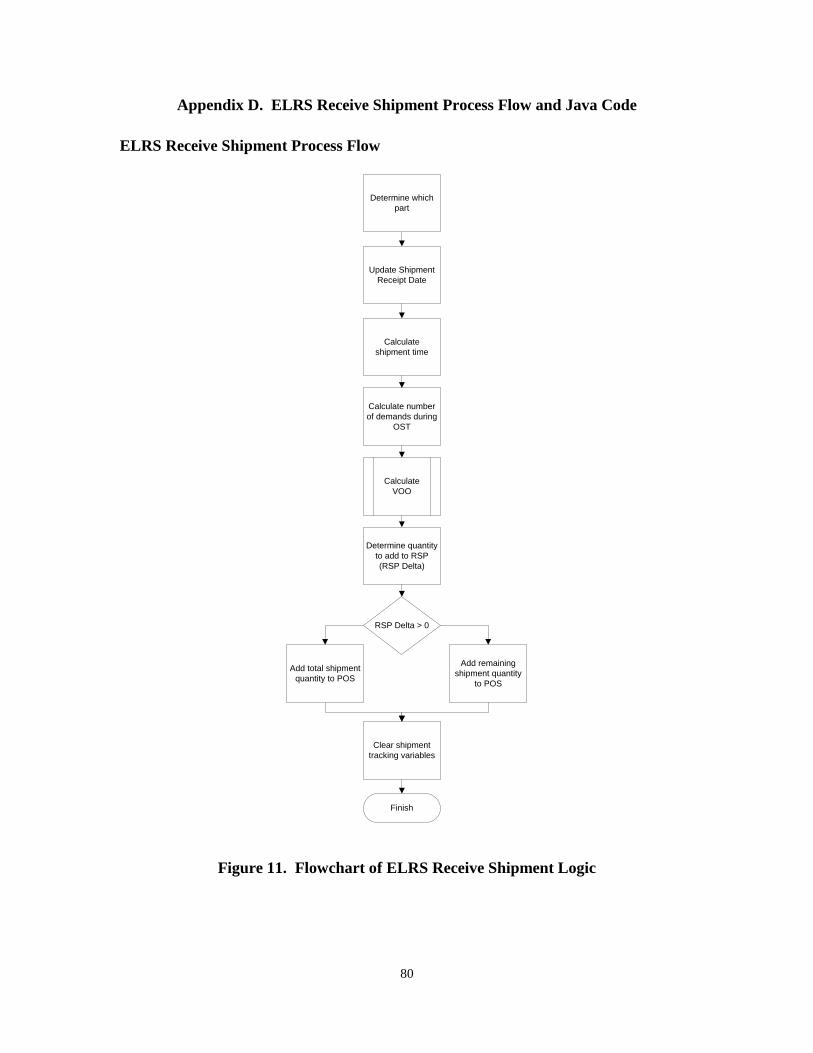
80
Appendix D. ELRS Receive Shipment Process Flow and Java Code
ELRS Receive Shipment Process Flow
Update Shipment Receipt Date
Calculate shipment time
Calculate number of demands during
OST
Clear shipment tracking variables
Calculate VOO
Determine which part
Determine quantity to add to RSP (RSP Delta)
RSP Delta > 0
Add remaining shipment quantity
to POS
Add total shipment quantity to POS
Finish
Figure 11. Flowchart of ELRS Receive Shipment Logic
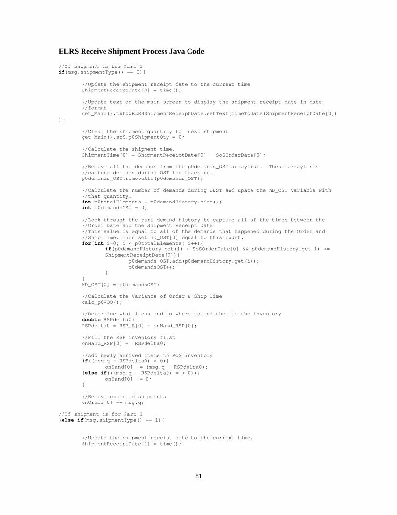
81
ELRS Receive Shipment Process Java Code
//If shipment is for Part 1 if(msg.shipmentType() == 0){ //Update the shipment receipt date to the current time ShipmentReceiptDate[0] = time();
//Update text on the main screen to display the shipment receipt date in date //format
get_Main().txtp0ELRSShipmentReceiptDate.setText(timeToDate(ShipmentReceiptDate[0])); //Clear the shipment quantity for next shipment get_Main().soS.p0ShipmentQty = 0; //Calculate the shipment time. ShipmentTime[0] = ShipmentReceiptDate[0] - SoSOrderDate[0];
//Remove all the demands from the p0demands_OST arraylist. These arraylists //capture demands during OST for tracking.
p0demands_OST.removeAll(p0demands_OST);
//Calculate the number of demands during O&ST and upate the nD_OST variable with //that quantity.
int p0totalElements = p0demandHistory.size(); int p0demandsOST = 0;
//Look through the part demand history to capture all of the times between the //Order Date and the Shipment Receipt Date //This value is equal to all of the demands that happened during the Order and //Ship Time. Then set nD_OST[0] equal to this count.
for(int i=0; i < p0totalElements; i++){ if(p0demandHistory.get(i) > SoSOrderDate[0] && p0demandHistory.get(i) <= ShipmentReceiptDate[0]){
p0demands_OST.add(p0demandHistory.get(i)); p0demandsOST++; } } ND_OST[0] = p0demandsOST; //Calculate the Variance of Order & Ship Time calc_p0VOO(); //Determine what items and to where to add them to the inventory double RSPdelta0; RSPdelta0 = RSP_S[0] - onHand_RSP[0]; //Fill the RSP inventory first onHand_RSP[0] += RSPdelta0; //Add newly arrived items to POS inventory if((msg.q - RSPdelta0) > 0){ onHand[0] += (msg.q - RSPdelta0); }else if(((msg.q - RSPdelta0) = < 0)){ onHand[0] += 0; } //Remove expected shipments onOrder[0] -= msg.q; //If shipment is for Part 1 }else if(msg.shipmentType() == 1){ //Update the shipment receipt date to the current time. ShipmentReceiptDate[1] = time();
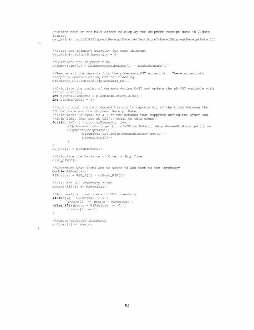
82
//Update text on the main screen to display the shipment receipt date in //date format.
get_Main().txtp1ELRSShipmentReceiptDate.setText(timeToDate(ShipmentReceiptDate[1])); //Clear the shipment quantity for next shipment get_Main().soS.p1ShipmentQty = 0; //Calculate the shipment time. ShipmentTime[1] = ShipmentReceiptDate[1] - SoSOrderDate[1];
//Remove all the demands from the p1demands_OST arraylist. These arraylists //capture demands during OST for tracking.
p1demands_OST.removeAll(p1demands_OST);
//Calculate the number of demands during O&ST and update the nD_OST variable with //that quantity.
int p1totalElements = p1demandHistory.size(); int p1demandsOST = 0;
//Look through the part demand history to capture all of the times between the //Order Date and the Shipment Receipt Date //This value is equal to all of the demands that happened during the Order and //Ship Time. Then set nD_OST[1] equal to this count.
for(int i=0; i < p1totalElements; i++){ if(p1demandHistory.get(i) > SoSOrderDate[1] && p1demandHistory.get(i) <= ShipmentReceiptDate[1]){
p1demands_OST.add(p1demandHistory.get(i)); p1demandsOST++; } } ND_OST[1] = p1demandsOST; //Calculate the Variance of Order & Ship Time. calc_p1VOO(); //Determine what items and to where to add them to the inventory double RSPdelta1; RSPdelta1 = RSP_S[1] - onHand_RSP[1]; //Fill the RSP inventory first onHand_RSP[1] += RSPdelta1; //Add newly arrived items to POS inventory if((msg.q - RSPdelta1) > 0){ onHand[1] += (msg.q - RSPdelta1); }else if(((msg.q - RSPdelta1) =< 0)){ onHand[1] += 0; } //Remove expected shipments onOrder[1] -= msg.q; }
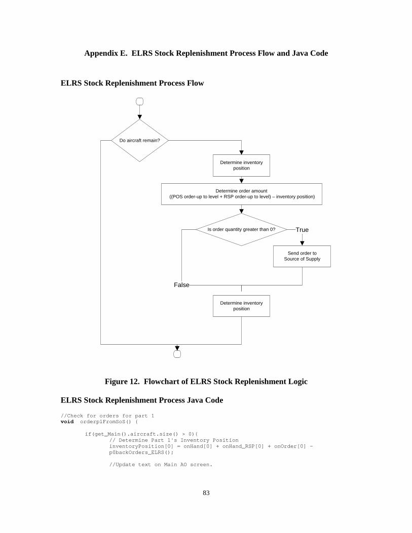
83
Appendix E. ELRS Stock Replenishment Process Flow and Java Code
ELRS Stock Replenishment Process Flow
Determine inventory position
Determine order amount ((POS order-up to level + RSP order-up to level) – inventory position)
Is order quantity greater than 0?
Send order toSource of Supply
Determine inventory position
True
False
Do aircraft remain?
Figure 12. Flowchart of ELRS Stock Replenishment Logic
ELRS Stock Replenishment Process Java Code
//Check for orders for part 1 void orderp1FromSoS() {
if(get_Main().aircraft.size() > 0){ // Determine Part 1's Inventory Position inventoryPosition[0] = onHand[0] + onHand_RSP[0] + onOrder[0] – p0backOrders_ELRS(); //Update text on Main AO screen.
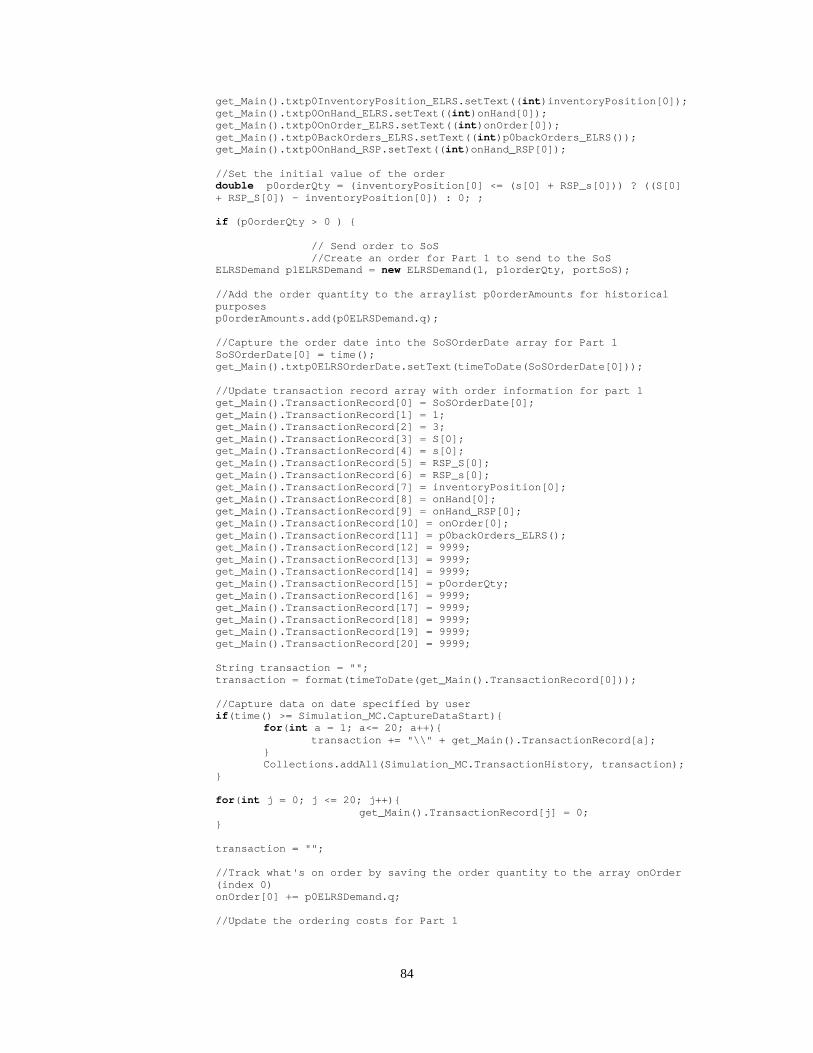
84
get_Main().txtp0InventoryPosition_ELRS.setText((int)inventoryPosition[0]); get_Main().txtp0OnHand_ELRS.setText((int)onHand[0]); get_Main().txtp0OnOrder_ELRS.setText((int)onOrder[0]); get_Main().txtp0BackOrders_ELRS.setText((int)p0backOrders_ELRS()); get_Main().txtp0OnHand_RSP.setText((int)onHand_RSP[0]); //Set the initial value of the order double p0orderQty = (inventoryPosition[0] <= (s[0] + RSP_s[0])) ? ((S[0] + RSP_S[0]) - inventoryPosition[0]) : 0; ; if (p0orderQty > 0 ) { // Send order to SoS //Create an order for Part 1 to send to the SoS ELRSDemand p1ELRSDemand = new ELRSDemand(1, p1orderQty, portSoS); //Add the order quantity to the arraylist p0orderAmounts for historical purposes p0orderAmounts.add(p0ELRSDemand.q); //Capture the order date into the SoSOrderDate array for Part 1 SoSOrderDate[0] = time(); get_Main().txtp0ELRSOrderDate.setText(timeToDate(SoSOrderDate[0])); //Update transaction record array with order information for part 1 get_Main().TransactionRecord[0] = SoSOrderDate[0]; get_Main().TransactionRecord[1] = 1; get_Main().TransactionRecord[2] = 3; get_Main().TransactionRecord[3] = S[0]; get_Main().TransactionRecord[4] = s[0]; get_Main().TransactionRecord[5] = RSP_S[0]; get_Main().TransactionRecord[6] = RSP_s[0]; get_Main().TransactionRecord[7] = inventoryPosition[0]; get_Main().TransactionRecord[8] = onHand[0]; get_Main().TransactionRecord[9] = onHand_RSP[0]; get_Main().TransactionRecord[10] = onOrder[0]; get_Main().TransactionRecord[11] = p0backOrders_ELRS(); get_Main().TransactionRecord[12] = 9999; get_Main().TransactionRecord[13] = 9999; get_Main().TransactionRecord[14] = 9999; get_Main().TransactionRecord[15] = p0orderQty; get_Main().TransactionRecord[16] = 9999; get_Main().TransactionRecord[17] = 9999; get_Main().TransactionRecord[18] = 9999; get_Main().TransactionRecord[19] = 9999; get_Main().TransactionRecord[20] = 9999; String transaction = ""; transaction = format(timeToDate(get_Main().TransactionRecord[0])); //Capture data on date specified by user if(time() >= Simulation_MC.CaptureDataStart){ for(int a = 1; a<= 20; a++){ transaction += "\\" + get_Main().TransactionRecord[a]; } Collections.addAll(Simulation_MC.TransactionHistory, transaction); } for(int j = 0; j <= 20; j++){ get_Main().TransactionRecord[j] = 0; } transaction = ""; //Track what's on order by saving the order quantity to the array onOrder (index 0) onOrder[0] += p0ELRSDemand.q; //Update the ordering costs for Part 1

85
orderCosts[0] += OrderingCost[0]; //Track the total number of orders for Part 1 numberOfOrders[0]++; //Track what's on order by saving the order quantity to array onOrder (index 0) onOrder[0] += p0ELRSDemand.q; //Send the order to the SoS portSoS.send(p0ELRSDemand); //Clear the order quantity value from the variable p0orderQty for the next order p0orderQty = 0; //Update the ordering costs for Part 1 orderCosts[0] += OrderingCost[0]; //Track the total number of orders for Part 1 numberOfOrders[0]++; } // Determine Part 1's Inventory Position inventoryPosition[0] = onHand[0] + onHand_RSP[0] + onOrder[0] – p0backOrders_ELRS(); //Update text on main screen. get_Main().txtp0InventoryPosition_ELRS.setText((int)inventoryPosition[0]); get_Main().txtp0OnHand_ELRS.setText((int)onHand[0]); get_Main().txtp0OnOrder_ELRS.setText((int)onOrder[0]); get_Main().txtp0BackOrders_ELRS.setText((int)p0backOrders_ELRS()); get_Main().txtp0OnHand_RSP.setText((int)onHand_RSP[0]);
}
return; }
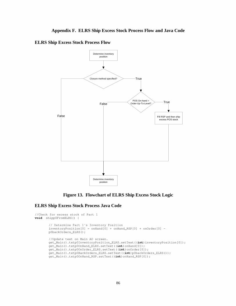
86
Appendix F. ELRS Ship Excess Stock Process Flow and Java Code
ELRS Ship Excess Stock Process Flow
Determine inventory position
Closure method specified?
Determine inventory position
True
False
POS On-hand > Order-Up-To-Level? TrueFalse
Fill RSP and then ship excess POS stock
Figure 13. Flowchart of ELRS Ship Excess Stock Logic
ELRS Ship Excess Stock Process Java Code
//Check for excess stock of Part 1 void shipp0FromELRS() { // Determine Part 1's Inventory Position
inventoryPosition[0] = onHand[0] + onHand_RSP[0] + onOrder[0] - p0backOrders_ELRS();
//Update text on Main AO screen. get_Main().txtp0InventoryPosition_ELRS.setText((int)inventoryPosition[0]); get_Main().txtp0OnHand_ELRS.setText((int)onHand[0]); get_Main().txtp0OnOrder_ELRS.setText((int)onOrder[0]); get_Main().txtp0BackOrders_ELRS.setText((int)p0backOrders_ELRS()); get_Main().txtp0OnHand_RSP.setText((int)onHand_RSP[0]);
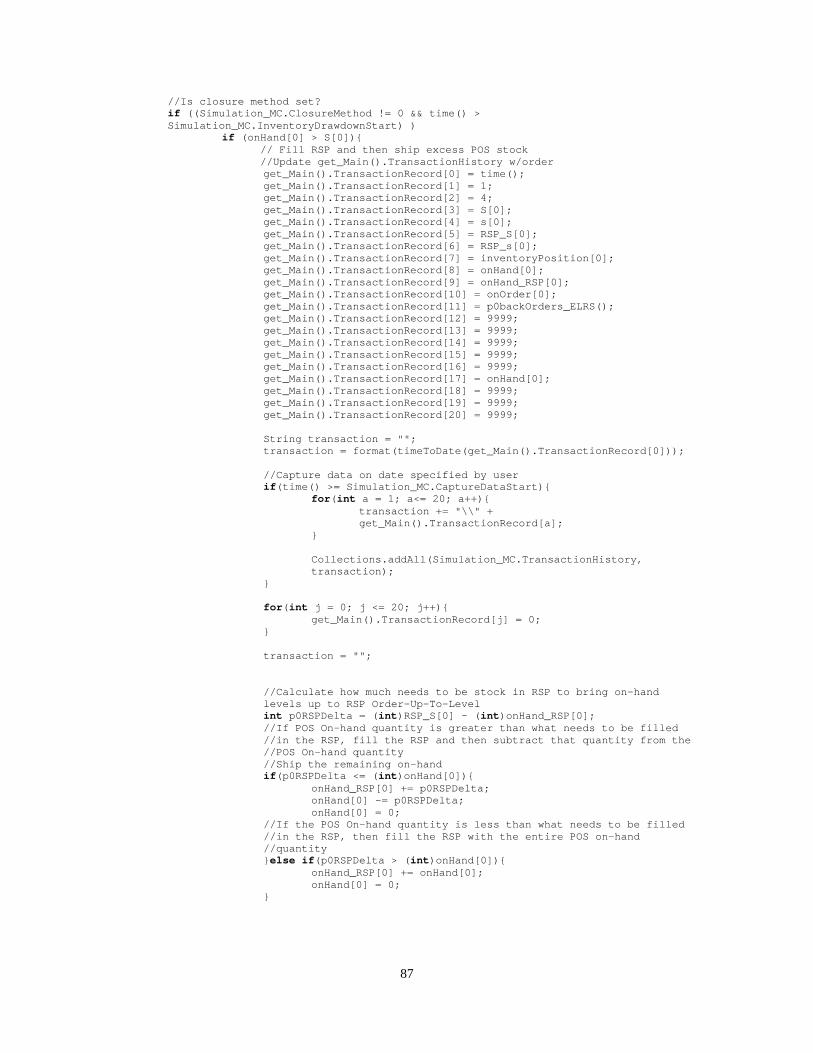
87
//Is closure method set? if ((Simulation_MC.ClosureMethod != 0 && time() > Simulation_MC.InventoryDrawdownStart) )
if (onHand[0] > S[0]){ // Fill RSP and then ship excess POS stock //Update get_Main().TransactionHistory w/order
get_Main().TransactionRecord[0] = time(); get_Main().TransactionRecord[1] = 1; get_Main().TransactionRecord[2] = 4; get_Main().TransactionRecord[3] = S[0]; get_Main().TransactionRecord[4] = s[0]; get_Main().TransactionRecord[5] = RSP_S[0]; get_Main().TransactionRecord[6] = RSP_s[0]; get_Main().TransactionRecord[7] = inventoryPosition[0]; get_Main().TransactionRecord[8] = onHand[0]; get_Main().TransactionRecord[9] = onHand_RSP[0]; get_Main().TransactionRecord[10] = onOrder[0]; get_Main().TransactionRecord[11] = p0backOrders_ELRS(); get_Main().TransactionRecord[12] = 9999; get_Main().TransactionRecord[13] = 9999; get_Main().TransactionRecord[14] = 9999; get_Main().TransactionRecord[15] = 9999; get_Main().TransactionRecord[16] = 9999; get_Main().TransactionRecord[17] = onHand[0]; get_Main().TransactionRecord[18] = 9999; get_Main().TransactionRecord[19] = 9999; get_Main().TransactionRecord[20] = 9999;
String transaction = ""; transaction = format(timeToDate(get_Main().TransactionRecord[0]));
//Capture data on date specified by user if(time() >= Simulation_MC.CaptureDataStart){
for(int a = 1; a<= 20; a++){ transaction += "\\" + get_Main().TransactionRecord[a];
} Collections.addAll(Simulation_MC.TransactionHistory, transaction);
}
for(int j = 0; j <= 20; j++){ get_Main().TransactionRecord[j] = 0;
}
transaction = "";
//Calculate how much needs to be stock in RSP to bring on-hand levels up to RSP Order-Up-To-Level int p0RSPDelta = (int)RSP_S[0] - (int)onHand_RSP[0]; //If POS On-hand quantity is greater than what needs to be filled //in the RSP, fill the RSP and then subtract that quantity from the //POS On-hand quantity //Ship the remaining on-hand if(p0RSPDelta <= (int)onHand[0]){
onHand_RSP[0] += p0RSPDelta; onHand[0] -= p0RSPDelta; onHand[0] = 0;
//If the POS On-hand quantity is less than what needs to be filled //in the RSP, then fill the RSP with the entire POS on-hand //quantity }else if(p0RSPDelta > (int)onHand[0]){
onHand_RSP[0] += onHand[0]; onHand[0] = 0;
}
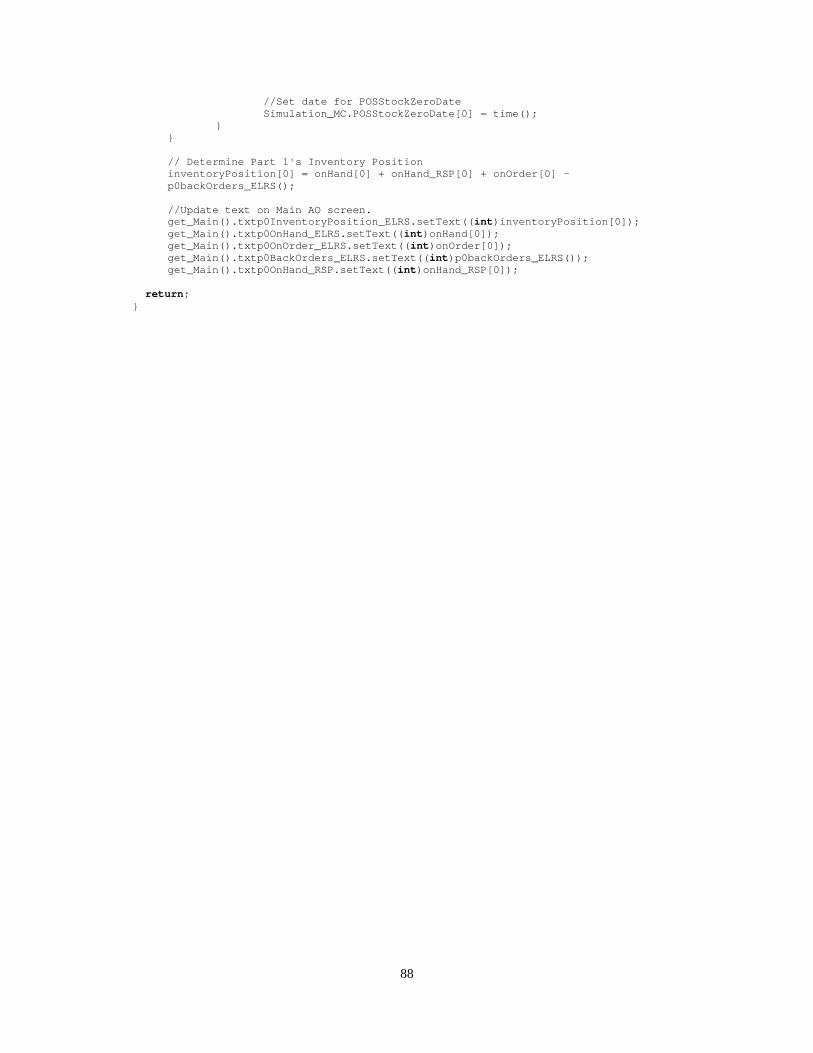
88
//Set date for POSStockZeroDate Simulation_MC.POSStockZeroDate[0] = time();
} } // Determine Part 1's Inventory Position
inventoryPosition[0] = onHand[0] + onHand_RSP[0] + onOrder[0] - p0backOrders_ELRS();
//Update text on Main AO screen. get_Main().txtp0InventoryPosition_ELRS.setText((int)inventoryPosition[0]); get_Main().txtp0OnHand_ELRS.setText((int)onHand[0]); get_Main().txtp0OnOrder_ELRS.setText((int)onOrder[0]); get_Main().txtp0BackOrders_ELRS.setText((int)p0backOrders_ELRS()); get_Main().txtp0OnHand_RSP.setText((int)onHand_RSP[0]);
return; }
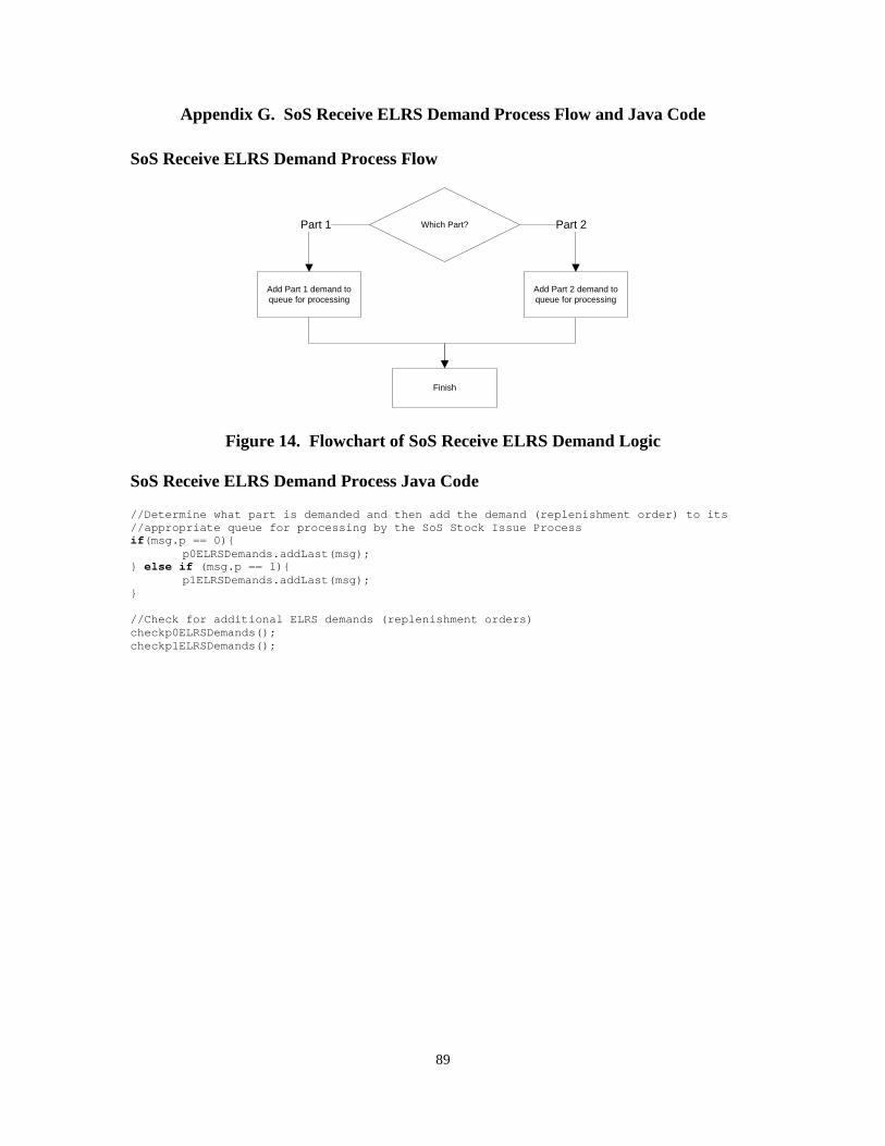
89
Appendix G. SoS Receive ELRS Demand Process Flow and Java Code
SoS Receive ELRS Demand Process Flow
Which Part?
Finish
Add Part 1 demand to queue for processing
Part 1
Add Part 2 demand to queue for processing
Part 2
Figure 14. Flowchart of SoS Receive ELRS Demand Logic
SoS Receive ELRS Demand Process Java Code
//Determine what part is demanded and then add the demand (replenishment order) to its //appropriate queue for processing by the SoS Stock Issue Process if(msg.p == 0){ p0ELRSDemands.addLast(msg); } else if (msg.p == 1){ p1ELRSDemands.addLast(msg); } //Check for additional ELRS demands (replenishment orders) checkp0ELRSDemands(); checkp1ELRSDemands();
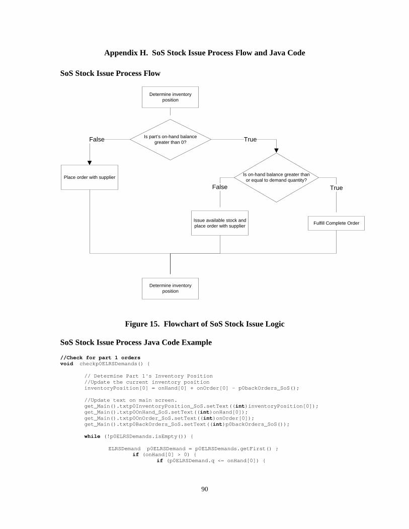
90
Appendix H. SoS Stock Issue Process Flow and Java Code
SoS Stock Issue Process Flow
Determine inventory position
Is part’s on-hand balance greater than 0?
Is on-hand balance greater than or equal to demand quantity?
Fulfill Complete OrderIssue available stock and place order with supplier
Determine inventory position
True
False True
Place order with supplier
False
Figure 15. Flowchart of SoS Stock Issue Logic
SoS Stock Issue Process Java Code Example
//Check for part 1 orders void checkp0ELRSDemands() {
// Determine Part 1's Inventory Position //Update the current inventory position inventoryPosition[0] = onHand[0] + onOrder[0] - p0backOrders_SoS(); //Update text on main screen. get_Main().txtp0InventoryPosition_SoS.setText((int)inventoryPosition[0]); get_Main().txtp0OnHand_SoS.setText((int)onHand[0]); get_Main().txtp0OnOrder_SoS.setText((int)onOrder[0]); get_Main().txtp0BackOrders_SoS.setText((int)p0backOrders_SoS()); while (!p0ELRSDemands.isEmpty()) {
ELRSDemand p0ELRSDemand = p0ELRSDemands.getFirst() ; if (onHand[0] > 0) {
if (p0ELRSDemand.q <= onHand[0]) {
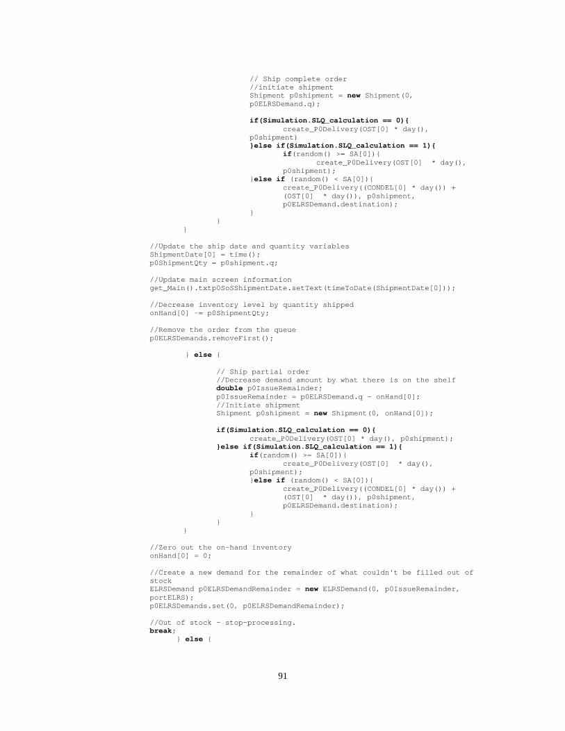
91
// Ship complete order //initiate shipment
Shipment p0shipment = new Shipment(0, p0ELRSDemand.q); if(Simulation.SLQ_calculation == 0){ create_P0Delivery(OST[0] * day(), p0shipment) }else if(Simulation.SLQ_calculation == 1){
if(random() >= SA[0]){ create_P0Delivery(OST[0] * day(),
p0shipment); }else if (random() < SA[0]){
create_P0Delivery((CONDEL[0] * day()) + (OST[0] * day()), p0shipment, p0ELRSDemand.destination);
} }
} //Update the ship date and quantity variables ShipmentDate[0] = time(); p0ShipmentQty = p0shipment.q; //Update main screen information get_Main().txtp0SoSShipmentDate.setText(timeToDate(ShipmentDate[0])); //Decrease inventory level by quantity shipped onHand[0] -= p0ShipmentQty; //Remove the order from the queue p0ELRSDemands.removeFirst(); } else { // Ship partial order //Decrease demand amount by what there is on the shelf
double p0IssueRemainder; p0IssueRemainder = p0ELRSDemand.q - onHand[0]; //Initiate shipment Shipment p0shipment = new Shipment(0, onHand[0]); if(Simulation.SLQ_calculation == 0){ create_P0Delivery(OST[0] * day(), p0shipment); }else if(Simulation.SLQ_calculation == 1){
if(random() >= SA[0]){ create_P0Delivery(OST[0] * day(),
p0shipment); }else if (random() < SA[0]){
create_P0Delivery((CONDEL[0] * day()) + (OST[0] * day()), p0shipment, p0ELRSDemand.destination);
} }
} //Zero out the on-hand inventory onHand[0] = 0; //Create a new demand for the remainder of what couldn't be filled out of stock ELRSDemand p0ELRSDemandRemainder = new ELRSDemand(0, p0IssueRemainder, portELRS); p0ELRSDemands.set(0, p0ELRSDemandRemainder); //Out of stock - stop-processing. break; } else {
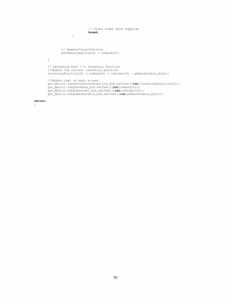
92
// Place order with supplier break; } // UpdateVisualControls p0OnHand_Replicator = onHand[0];
} // Determine Part 1's Inventory Position //Update the current inventory position inventoryPosition[0] = onHand[0] + onOrder[0] - p0backOrders_SoS(); //Update text on main screen get_Main().txtp0InventoryPosition_SoS.setText((int)inventoryPosition[0]); get_Main().txtp0OnHand_SoS.setText((int)onHand[0]); get_Main().txtp0OnOrder_SoS.setText((int)onOrder[0]); get_Main().txtp0BackOrders_SoS.setText((int)p0backOrders_SoS());
return; }
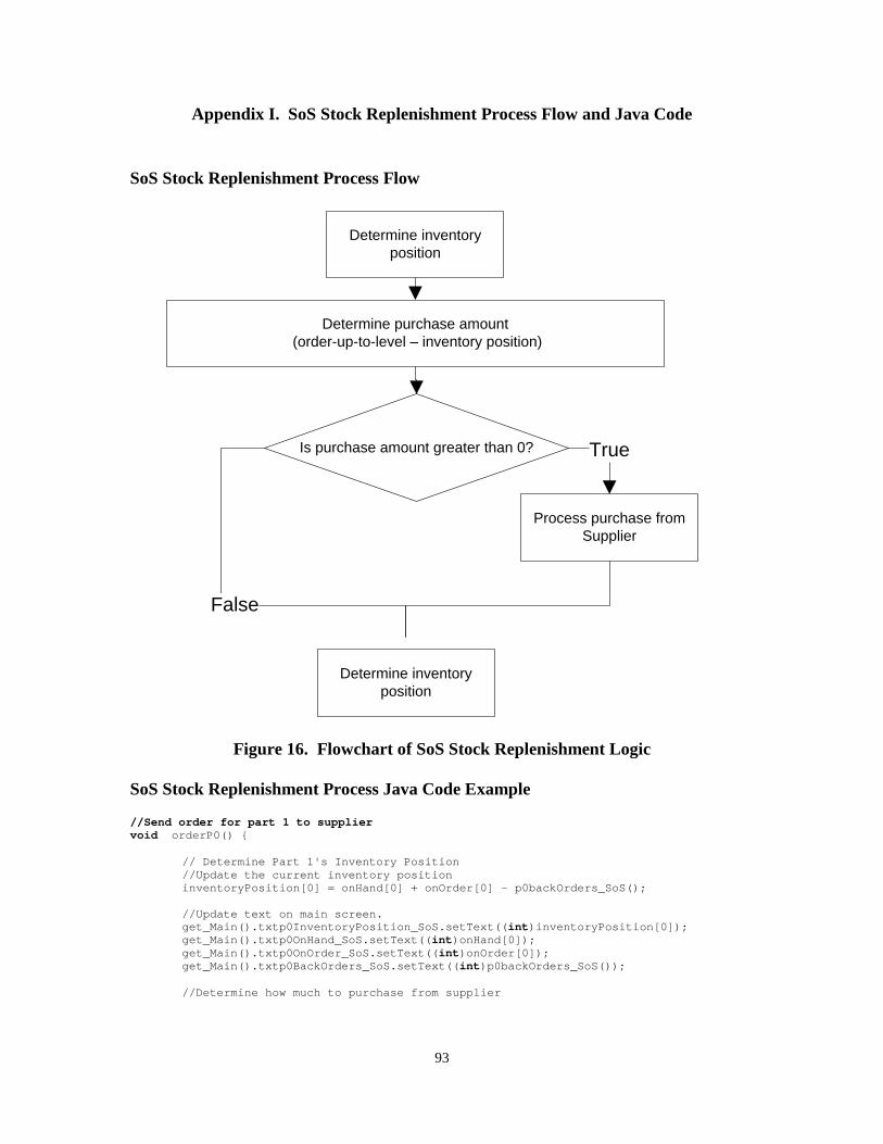
93
Appendix I. SoS Stock Replenishment Process Flow and Java Code
SoS Stock Replenishment Process Flow
Determine inventory position
Determine purchase amount (order-up-to-level – inventory position)
Is purchase amount greater than 0?
Process purchase from Supplier
Determine inventory position
True
False
Figure 16. Flowchart of SoS Stock Replenishment Logic
SoS Stock Replenishment Process Java Code Example
//Send order for part 1 to supplier void orderP0() {
// Determine Part 1's Inventory Position //Update the current inventory position inventoryPosition[0] = onHand[0] + onOrder[0] - p0backOrders_SoS(); //Update text on main screen. get_Main().txtp0InventoryPosition_SoS.setText((int)inventoryPosition[0]); get_Main().txtp0OnHand_SoS.setText((int)onHand[0]); get_Main().txtp0OnOrder_SoS.setText((int)onOrder[0]); get_Main().txtp0BackOrders_SoS.setText((int)p0backOrders_SoS()); //Determine how much to purchase from supplier
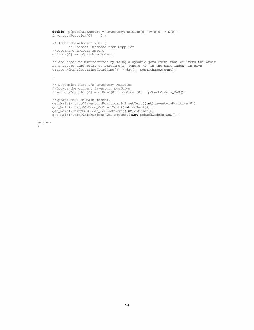
94
double p0purchaseAmount = inventoryPosition[0] <= s[0] ? S[0] - inventoryPosition[0] : 0 ; if (p0purchaseAmount > 0) { // Process Purchase from Supplier //Determine onOrder amount onOrder[0] += p0purchaseAmount; //Send order to manufacturer by using a dynamic java event that delivers the order at a future time equal to leadTime[i] (where “I” is the part index) in days create_P0Manufacturing(leadTime[0] * day(), p0purchaseAmount); } // Determine Part 1's Inventory Position //Update the current inventory position inventoryPosition[0] = onHand[0] + onOrder[0] - p0backOrders_SoS(); //Update text on main screen. get_Main().txtp0InventoryPosition_SoS.setText((int)inventoryPosition[0]); get_Main().txtp0OnHand_SoS.setText((int)onHand[0]); get_Main().txtp0OnOrder_SoS.setText((int)onOrder[0]); get_Main().txtp0BackOrders_SoS.setText((int)p0backOrders_SoS());
return; }
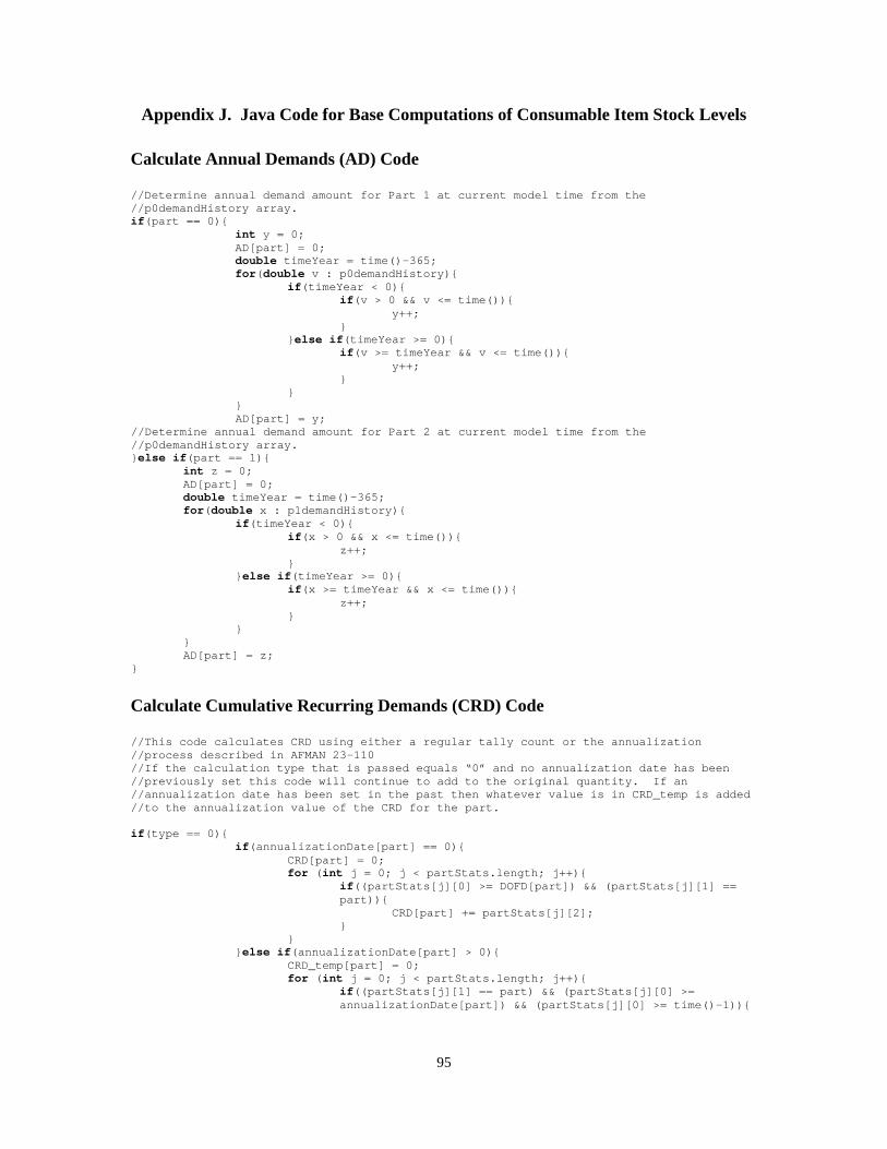
95
Appendix J. Java Code for Base Computations of Consumable Item Stock Levels
Calculate Annual Demands (AD) Code //Determine annual demand amount for Part 1 at current model time from the //p0demandHistory array. if(part == 0){ int y = 0; AD[part] = 0; double timeYear = time()-365; for(double v : p0demandHistory){ if(timeYear < 0){ if(v > 0 && v <= time()){ y++; } }else if(timeYear >= 0){ if(v >= timeYear && v <= time()){ y++; } } } AD[part] = y; //Determine annual demand amount for Part 2 at current model time from the //p0demandHistory array. }else if(part == 1){ int z = 0; AD[part] = 0; double timeYear = time()-365; for(double x : p1demandHistory){ if(timeYear < 0){ if(x > 0 && x <= time()){ z++; } }else if(timeYear >= 0){ if(x >= timeYear && x <= time()){ z++; } } } AD[part] = z; }
Calculate Cumulative Recurring Demands (CRD) Code //This code calculates CRD using either a regular tally count or the annualization //process described in AFMAN 23-110 //If the calculation type that is passed equals “0” and no annualization date has been //previously set this code will continue to add to the original quantity. If an //annualization date has been set in the past then whatever value is in CRD_temp is added //to the annualization value of the CRD for the part. if(type == 0){ if(annualizationDate[part] == 0){ CRD[part] = 0; for (int j = 0; j < partStats.length; j++){
if((partStats[j][0] >= DOFD[part]) && (partStats[j][1] == part)){
CRD[part] += partStats[j][2]; } } }else if(annualizationDate[part] > 0){ CRD_temp[part] = 0; for (int j = 0; j < partStats.length; j++){
if((partStats[j][1] == part) && (partStats[j][0] >= annualizationDate[part]) && (partStats[j][0] >= time()-1)){

96
CRD_temp[part] += partStats[j][2]; } } CRD[part] += CRD_temp[part]; } //If the calculation type passed is equal to “1” then an annualized value of the CRD is //calculated. }else if(type == 1){ calcDDR(part); CRD[part] = (int)(DDR[part] * 365); }
Calculate Cumulative Demand Quantity (CDQ) and Cumulative Demand Quantity Squared (CDQ2) //This code calculates CDQ and CDQ2 using either a regular tally counts or the //annualization process described in AFMAN 23-110. If the calculation type that is //passed equals “0” and no annualization date has been previously set this code will //continue to add to the original quantity. If an annualization date has been set in the //past then whatever value is in CDQ_temp is added to the annualization value of the CDQ //value for the part. CDQ2 is then calculated off of the CDQ value for the respective /part.
if(type == 0){ if(annualizationDate[part] == 0){ CDQ[part] = 0; for (int j = 0; j < partStats.length; j++){
if((partStats[j][0] >= DOFD[part]) && (partStats[j][1] == part)){
CDQ[part] += partStats[j][2]; } } CDQ2[part] = (int)(pow(CDQ[part],2)); }else if(annualizationDate[part] > 0){ CDQ_temp[part] = 0; for (int j = 0; j < partStats.length; j++){
if((partStats[j][1] == part) && (partStats[j][0] >= annualizationDate[part]) && (partStats[j][0] >= time()-1)){
CDQ_temp[part] += partStats[j][2]; } } CDQ[part] += CDQ_temp[part]; CDQ2[part] = (int)(pow(CDQ[part],2)); } //If the calculation type passed is equal to “1” then an annualized value of the CDQ and CDQ2 is calculated for the part. }else if(type == 1){ CDQ[part] = CDQ[part]/(time()-DOFD[part]); CDQ[part] = (int)(CDQ[part] * 365); calcVOD(part); CDQ2[part] = (int)((365 * VOD[part]) + pow(CDQ[part],2)/365); }
Daily Demand Rate (DDR) Code //DDR formula as specified in AFMAN 23-110, Volume 2, Part 2, Chapter 19, Paragraph //19.2.1.1.1. //DDR is the average quantity of an item that is used daily. It’s simply the cumulative //recurring demands (CRD) divided by the number of days between the current date and the //date of first demand (DOFD)

97
//As specified in the AFMAN, if the difference, in days, between the current date and the //DOFD is less than 180 or greater than 540, then value of 180 and 540, respectively, are //used as the denominator value if(time()-DOFD[i] < 180){ DDR[i] = (CRD[i] / 180); }else if(time()-DOFD[i] >= 180 && time() - DOFD[i] < 540){ DDR[i] = (CRD[i] / (time() - DOFD[i])); }else if(time()-DOFD[i] >= 180 && time()-DOFD[i] >=540){ DDR[i] = (CRD[i] / 540); }
Daily Demand Frequency Rate (DDFR) Code //DDFR formula as specified in AFMAN 23-110, Volume 2, Part 2, Chapter 19, Paragraph //19.2.1.1.4. DDFR is the average daily number of customer demands for a part. DDFR is //also known as the demand arrival rate. DDFR is calculated by dividing the sum of the //number of demands in the current period (ND_CP), number of demands occurring between 6 //to 12 months in the past (ND_PSM1), and the number of demands that occurred between 12 //to 18 months in the past (ND_PSM2) by the difference, in days, between the current date //and the DOFD. This code does essentially the same process, but just with a moving 18-//month window. int DemandCount0 = 0; int DemandCount1 = 0; double DateDiff0 = time() - DOFD[0]; double DateDiff1 = time() - DOFD[1]; double denominator = 365; double denominator1 = 540; if(part == 0){ for(double v : p0demandHistory){ if(v > DOFD[0] && v <= time()){ DemandCount0++; } } if(DemandCount0 >= 1){ if(DateDiff0 <= 365){ DDFR[0] = (DemandCount0/denominator); }else if(DateDiff0 > 365 && DateDiff0 < 540){ DDFR[0] = (DemandCount0/(time()-DOFD[0])); }else if(DateDiff0 >= 540){ DDFR[0] = (DemandCount0/denominator1); } } }if(part == 1){ for(double v : p1demandHistory){ if(v > DOFD[1] && v <= time()){ DemandCount1++; } } if(DateDiff1 <= 365){ DDFR[1] = (DemandCount1/denominator); }else if(DateDiff1 > 365 && DateDiff1 < 540){ DDFR[1] = (DemandCount1/(time()-DOFD[1])); }else if(DateDiff1 >= 540){ DDFR[1] = (DemandCount1/denominator1); } }
General Economic Order Quantity (EOQ) Model Code //EOQ formula as specified in AFMAN 23-110, Volume 2, Part 2, Chapter 19, Attachment 19B-//4, Figure 19B4.1 EOQ[i] = (int)pow((2*AD[i]*OrderingCost[i])/HoldingCost[i],.5);
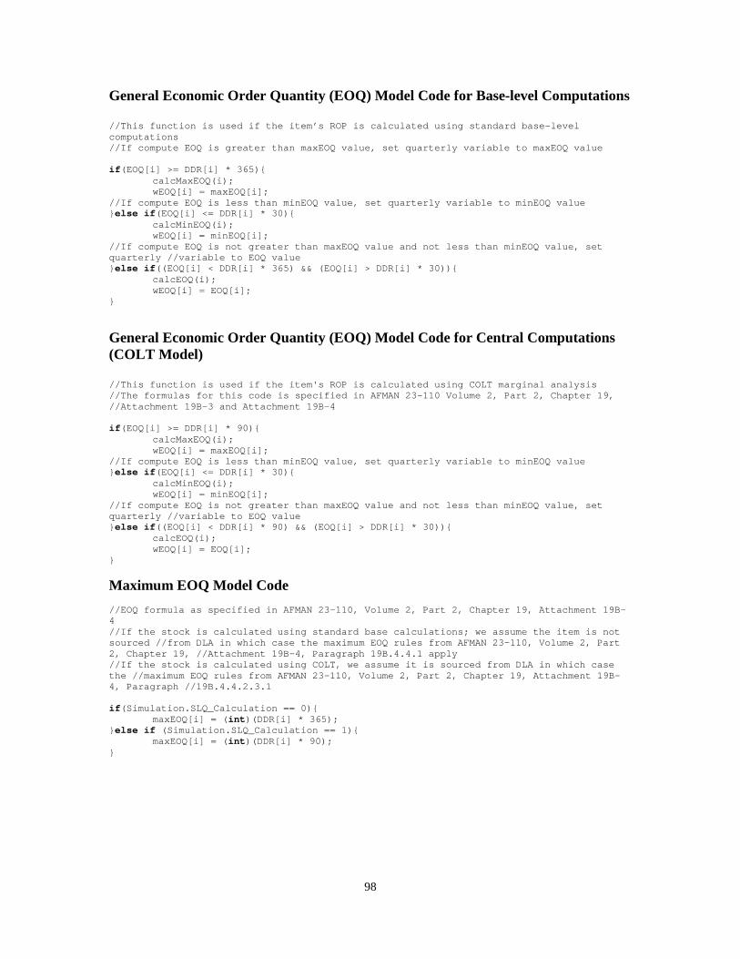
98
General Economic Order Quantity (EOQ) Model Code for Base-level Computations //This function is used if the item’s ROP is calculated using standard base-level computations //If compute EOQ is greater than maxEOQ value, set quarterly variable to maxEOQ value if(EOQ[i] >= DDR[i] * 365){ calcMaxEOQ(i); wEOQ[i] = maxEOQ[i]; //If compute EOQ is less than minEOQ value, set quarterly variable to minEOQ value }else if(EOQ[i] <= DDR[i] * 30){ calcMinEOQ(i); wEOQ[i] = minEOQ[i]; //If compute EOQ is not greater than maxEOQ value and not less than minEOQ value, set quarterly //variable to EOQ value }else if((EOQ[i] < DDR[i] * 365) && (EOQ[i] > DDR[i] * 30)){ calcEOQ(i); wEOQ[i] = EOQ[i]; }
General Economic Order Quantity (EOQ) Model Code for Central Computations (COLT Model) //This function is used if the item's ROP is calculated using COLT marginal analysis //The formulas for this code is specified in AFMAN 23-110 Volume 2, Part 2, Chapter 19, //Attachment 19B-3 and Attachment 19B-4 if(EOQ[i] >= DDR[i] * 90){ calcMaxEOQ(i); wEOQ[i] = maxEOQ[i]; //If compute EOQ is less than minEOQ value, set quarterly variable to minEOQ value }else if(EOQ[i] <= DDR[i] * 30){ calcMinEOQ(i); wEOQ[i] = minEOQ[i]; //If compute EOQ is not greater than maxEOQ value and not less than minEOQ value, set quarterly //variable to EOQ value }else if((EOQ[i] < DDR[i] * 90) && (EOQ[i] > DDR[i] * 30)){ calcEOQ(i); wEOQ[i] = EOQ[i]; }
Maximum EOQ Model Code //EOQ formula as specified in AFMAN 23-110, Volume 2, Part 2, Chapter 19, Attachment 19B-4 //If the stock is calculated using standard base calculations; we assume the item is not sourced //from DLA in which case the maximum EOQ rules from AFMAN 23-110, Volume 2, Part 2, Chapter 19, //Attachment 19B-4, Paragraph 19B.4.4.1 apply //If the stock is calculated using COLT, we assume it is sourced from DLA in which case the //maximum EOQ rules from AFMAN 23-110, Volume 2, Part 2, Chapter 19, Attachment 19B-4, Paragraph //19B.4.4.2.3.1 if(Simulation.SLQ_Calculation == 0){ maxEOQ[i] = (int)(DDR[i] * 365); }else if (Simulation.SLQ_Calculation == 1){ maxEOQ[i] = (int)(DDR[i] * 90); }
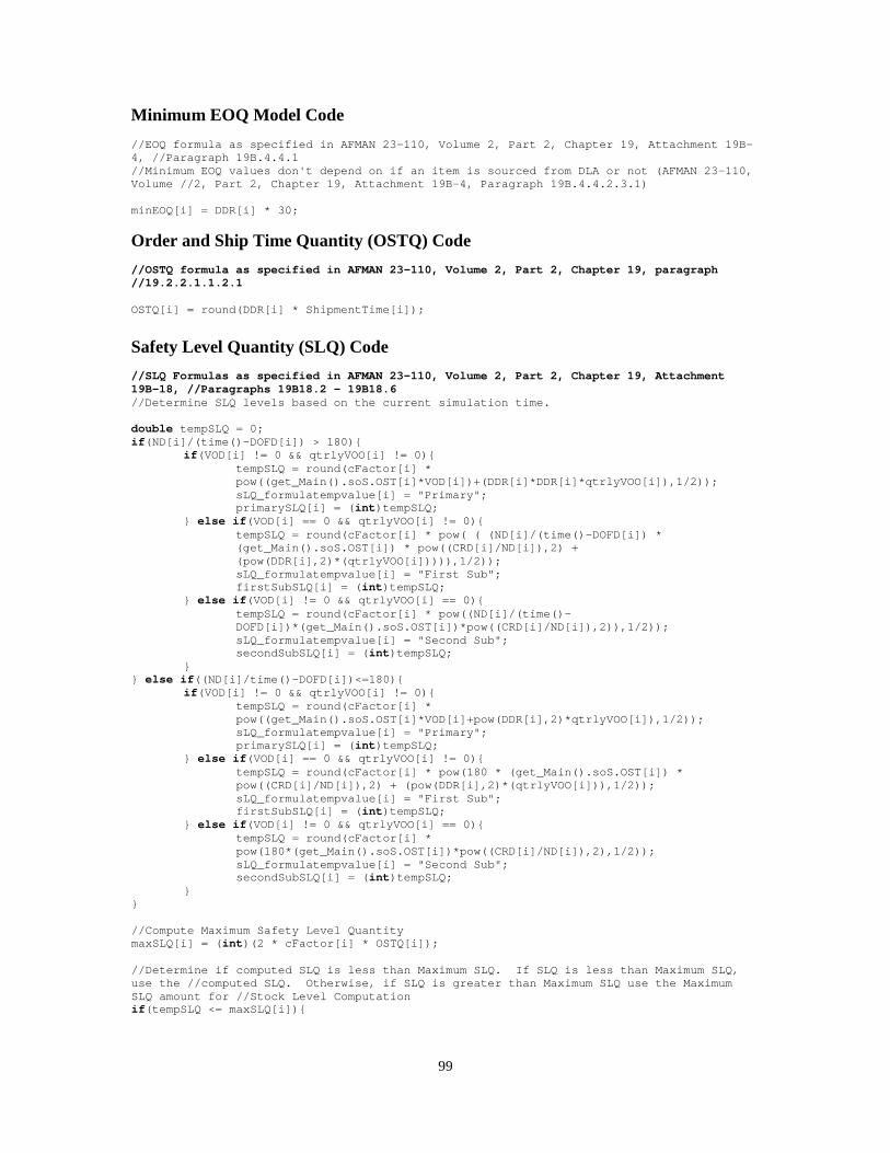
99
Minimum EOQ Model Code //EOQ formula as specified in AFMAN 23-110, Volume 2, Part 2, Chapter 19, Attachment 19B-4, //Paragraph 19B.4.4.1 //Minimum EOQ values don't depend on if an item is sourced from DLA or not (AFMAN 23-110, Volume //2, Part 2, Chapter 19, Attachment 19B-4, Paragraph 19B.4.4.2.3.1) minEOQ[i] = DDR[i] * 30;
Order and Ship Time Quantity (OSTQ) Code //OSTQ formula as specified in AFMAN 23-110, Volume 2, Part 2, Chapter 19, paragraph //19.2.2.1.1.2.1 OSTQ[i] = round(DDR[i] * ShipmentTime[i]);
Safety Level Quantity (SLQ) Code //SLQ Formulas as specified in AFMAN 23-110, Volume 2, Part 2, Chapter 19, Attachment 19B-18, //Paragraphs 19B18.2 – 19B18.6 //Determine SLQ levels based on the current simulation time. double tempSLQ = 0; if(ND[i]/(time()-DOFD[i]) > 180){ if(VOD[i] != 0 && qtrlyVOO[i] != 0){
tempSLQ = round(cFactor[i] * pow((get_Main().soS.OST[i]*VOD[i])+(DDR[i]*DDR[i]*qtrlyVOO[i]),1/2));
sLQ_formulatempvalue[i] = "Primary"; primarySLQ[i] = (int)tempSLQ; } else if(VOD[i] == 0 && qtrlyVOO[i] != 0){
tempSLQ = round(cFactor[i] * pow( ( (ND[i]/(time()-DOFD[i]) * (get_Main().soS.OST[i]) * pow((CRD[i]/ND[i]),2) + (pow(DDR[i],2)*(qtrlyVOO[i])))),1/2));
sLQ_formulatempvalue[i] = "First Sub"; firstSubSLQ[i] = (int)tempSLQ; } else if(VOD[i] != 0 && qtrlyVOO[i] == 0){
tempSLQ = round(cFactor[i] * pow((ND[i]/(time()-DOFD[i])*(get_Main().soS.OST[i])*pow((CRD[i]/ND[i]),2)),1/2));
sLQ_formulatempvalue[i] = "Second Sub"; secondSubSLQ[i] = (int)tempSLQ; } } else if((ND[i]/time()-DOFD[i])<=180){ if(VOD[i] != 0 && qtrlyVOO[i] != 0){
tempSLQ = round(cFactor[i] * pow((get_Main().soS.OST[i]*VOD[i]+pow(DDR[i],2)*qtrlyVOO[i]),1/2));
sLQ_formulatempvalue[i] = "Primary"; primarySLQ[i] = (int)tempSLQ; } else if(VOD[i] == 0 && qtrlyVOO[i] != 0){
tempSLQ = round(cFactor[i] * pow(180 * (get_Main().soS.OST[i]) * pow((CRD[i]/ND[i]),2) + (pow(DDR[i],2)*(qtrlyVOO[i])),1/2));
sLQ_formulatempvalue[i] = "First Sub"; firstSubSLQ[i] = (int)tempSLQ; } else if(VOD[i] != 0 && qtrlyVOO[i] == 0){
tempSLQ = round(cFactor[i] * pow(180*(get_Main().soS.OST[i])*pow((CRD[i]/ND[i]),2),1/2));
sLQ_formulatempvalue[i] = "Second Sub"; secondSubSLQ[i] = (int)tempSLQ; } } //Compute Maximum Safety Level Quantity maxSLQ[i] = (int)(2 * cFactor[i] * OSTQ[i]); //Determine if computed SLQ is less than Maximum SLQ. If SLQ is less than Maximum SLQ, use the //computed SLQ. Otherwise, if SLQ is greater than Maximum SLQ use the Maximum SLQ amount for //Stock Level Computation if(tempSLQ <= maxSLQ[i]){
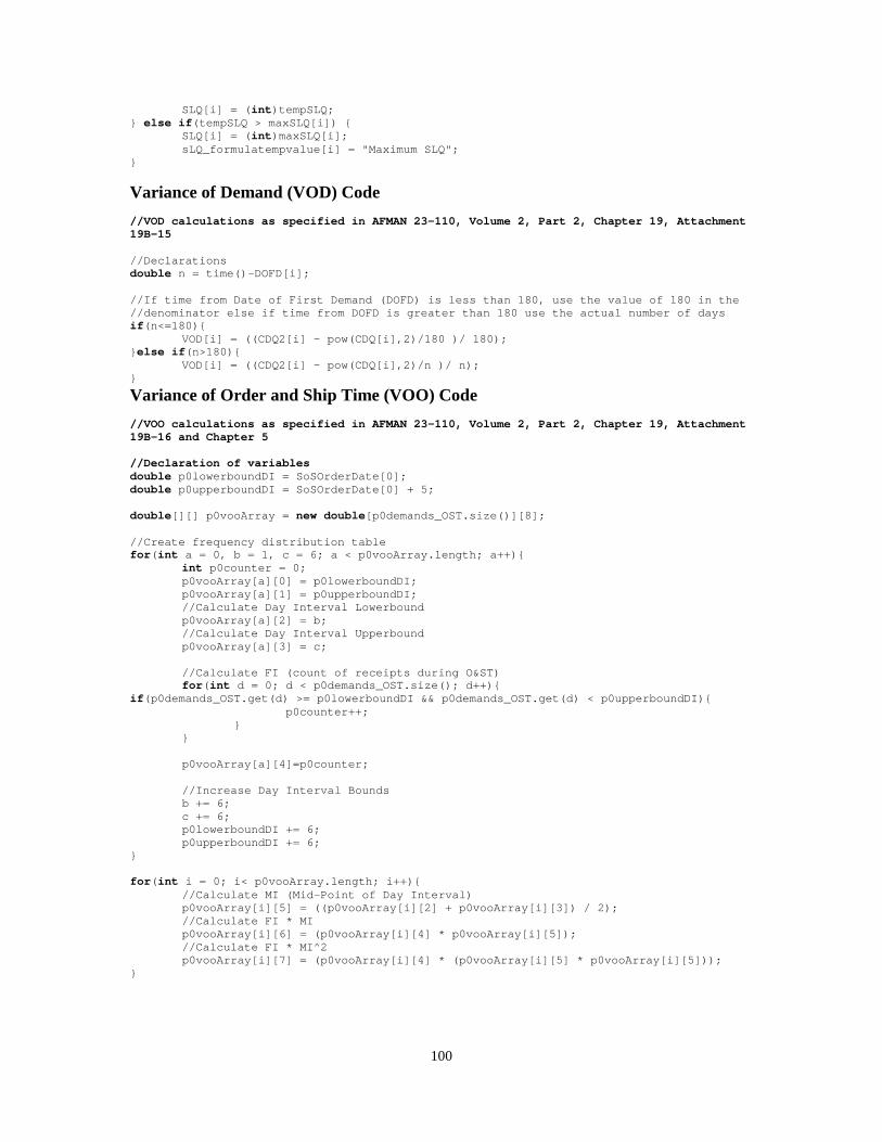
100
SLQ[i] = (int)tempSLQ; } else if(tempSLQ > maxSLQ[i]) { SLQ[i] = (int)maxSLQ[i]; sLQ_formulatempvalue[i] = "Maximum SLQ"; }
Variance of Demand (VOD) Code //VOD calculations as specified in AFMAN 23-110, Volume 2, Part 2, Chapter 19, Attachment 19B-15 //Declarations double n = time()-DOFD[i]; //If time from Date of First Demand (DOFD) is less than 180, use the value of 180 in the //denominator else if time from DOFD is greater than 180 use the actual number of days if(n<=180){ VOD[i] = ((CDQ2[i] - pow(CDQ[i],2)/180 )/ 180); }else if(n>180){ VOD[i] = ((CDQ2[i] - pow(CDQ[i],2)/n )/ n); }
Variance of Order and Ship Time (VOO) Code //VOO calculations as specified in AFMAN 23-110, Volume 2, Part 2, Chapter 19, Attachment 19B-16 and Chapter 5 //Declaration of variables double p0lowerboundDI = SoSOrderDate[0]; double p0upperboundDI = SoSOrderDate[0] + 5; double[][] p0vooArray = new double[p0demands_OST.size()][8]; //Create frequency distribution table for(int a = 0, b = 1, c = 6; a < p0vooArray.length; a++){ int p0counter = 0; p0vooArray[a][0] = p0lowerboundDI; p0vooArray[a][1] = p0upperboundDI; //Calculate Day Interval Lowerbound p0vooArray[a][2] = b; //Calculate Day Interval Upperbound p0vooArray[a][3] = c; //Calculate FI (count of receipts during O&ST) for(int d = 0; d < p0demands_OST.size(); d++){ if(p0demands_OST.get(d) >= p0lowerboundDI && p0demands_OST.get(d) < p0upperboundDI){ p0counter++; } } p0vooArray[a][4]=p0counter; //Increase Day Interval Bounds b += 6; c += 6; p0lowerboundDI += 6; p0upperboundDI += 6; } for(int i = 0; i< p0vooArray.length; i++){ //Calculate MI (Mid-Point of Day Interval) p0vooArray[i][5] = ((p0vooArray[i][2] + p0vooArray[i][3]) / 2); //Calculate FI * MI p0vooArray[i][6] = (p0vooArray[i][4] * p0vooArray[i][5]); //Calculate FI * MI^2 p0vooArray[i][7] = (p0vooArray[i][4] * (p0vooArray[i][5] * p0vooArray[i][5])); }
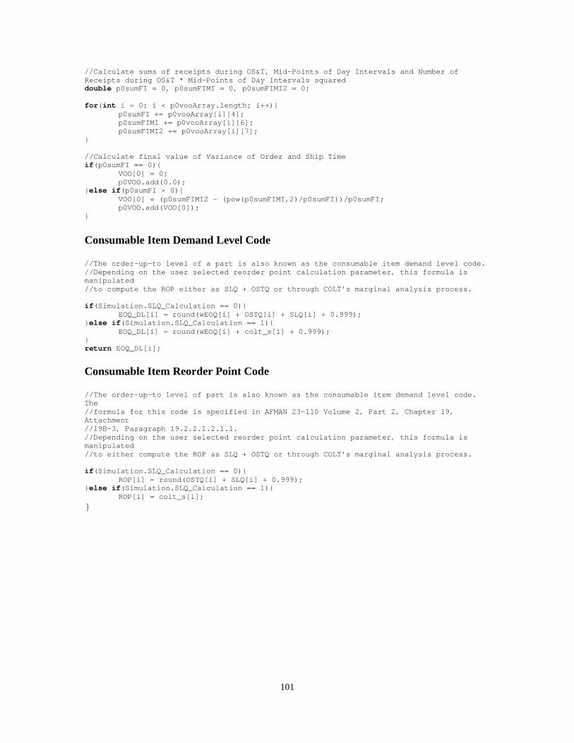
101
//Calculate sums of receipts during OS&T, Mid-Points of Day Intervals and Number of Receipts during OS&T * Mid-Points of Day Intervals squared double p0sumFI = 0, p0sumFIMI = 0, p0sumFIMI2 = 0; for(int i = 0; i < p0vooArray.length; i++){ p0sumFI += p0vooArray[i][4]; p0sumFIMI += p0vooArray[i][6]; p0sumFIMI2 += p0vooArray[i][7]; } //Calculate final value of Variance of Order and Ship Time if(p0sumFI == 0){ VOO[0] = 0; p0VOO.add(0.0); }else if(p0sumFI > 0){ VOO[0] = (p0sumFIMI2 - (pow(p0sumFIMI,2)/p0sumFI))/p0sumFI; p0VOO.add(VOO[0]); }
Consumable Item Demand Level Code //The order-up-to level of a part is also known as the consumable item demand level code. //Depending on the user selected reorder point calculation parameter, this formula is manipulated //to compute the ROP either as SLQ + OSTQ or through COLT’s marginal analysis process. if(Simulation.SLQ_Calculation == 0){ EOQ_DL[i] = round(wEOQ[i] + OSTQ[i] + SLQ[i] + 0.999); }else if(Simulation.SLQ_Calculation == 1){ EOQ_DL[i] = round(wEOQ[i] + colt_s[i] + 0.999); } return EOQ_DL[i]; Consumable Item Reorder Point Code //The order-up-to level of part is also known as the consumable item demand level code. The //formula for this code is specified in AFMAN 23-110 Volume 2, Part 2, Chapter 19, Attachment //19B-3, Paragraph 19.2.2.1.2.1.1. //Depending on the user selected reorder point calculation parameter, this formula is manipulated //to either compute the ROP as SLQ + OSTQ or through COLT’s marginal analysis process. if(Simulation.SLQ_Calculation == 0){ ROP[i] = round(OSTQ[i] + SLQ[i] + 0.999); }else if(Simulation.SLQ_Calculation == 1){ ROP[i] = colt_s[i];
}
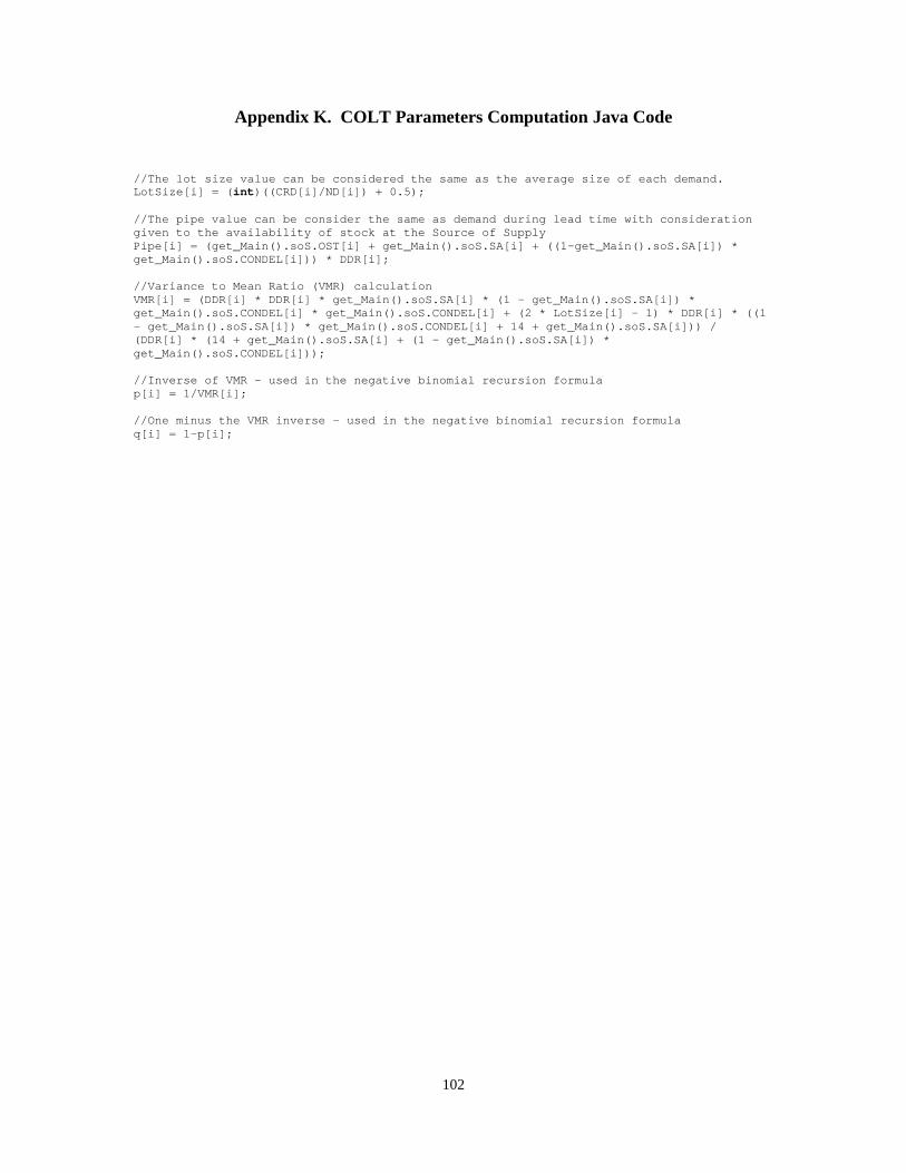
102
Appendix K. COLT Parameters Computation Java Code
//The lot size value can be considered the same as the average size of each demand. LotSize[i] = (int)((CRD[i]/ND[i]) + 0.5); //The pipe value can be consider the same as demand during lead time with consideration given to the availability of stock at the Source of Supply Pipe[i] = (get_Main().soS.OST[i] + get_Main().soS.SA[i] + ((1-get_Main().soS.SA[i]) * get_Main().soS.CONDEL[i])) * DDR[i]; //Variance to Mean Ratio (VMR) calculation VMR[i] = (DDR[i] * DDR[i] * get_Main().soS.SA[i] * (1 - get_Main().soS.SA[i]) * get_Main().soS.CONDEL[i] * get_Main().soS.CONDEL[i] + (2 * LotSize[i] - 1) * DDR[i] * ((1 - get_Main().soS.SA[i]) * get_Main().soS.CONDEL[i] + 14 + get_Main().soS.SA[i])) / (DDR[i] * (14 + get_Main().soS.SA[i] + (1 - get_Main().soS.SA[i]) * get_Main().soS.CONDEL[i])); //Inverse of VMR – used in the negative binomial recursion formula p[i] = 1/VMR[i]; //One minus the VMR inverse – used in the negative binomial recursion formula q[i] = 1-p[i];
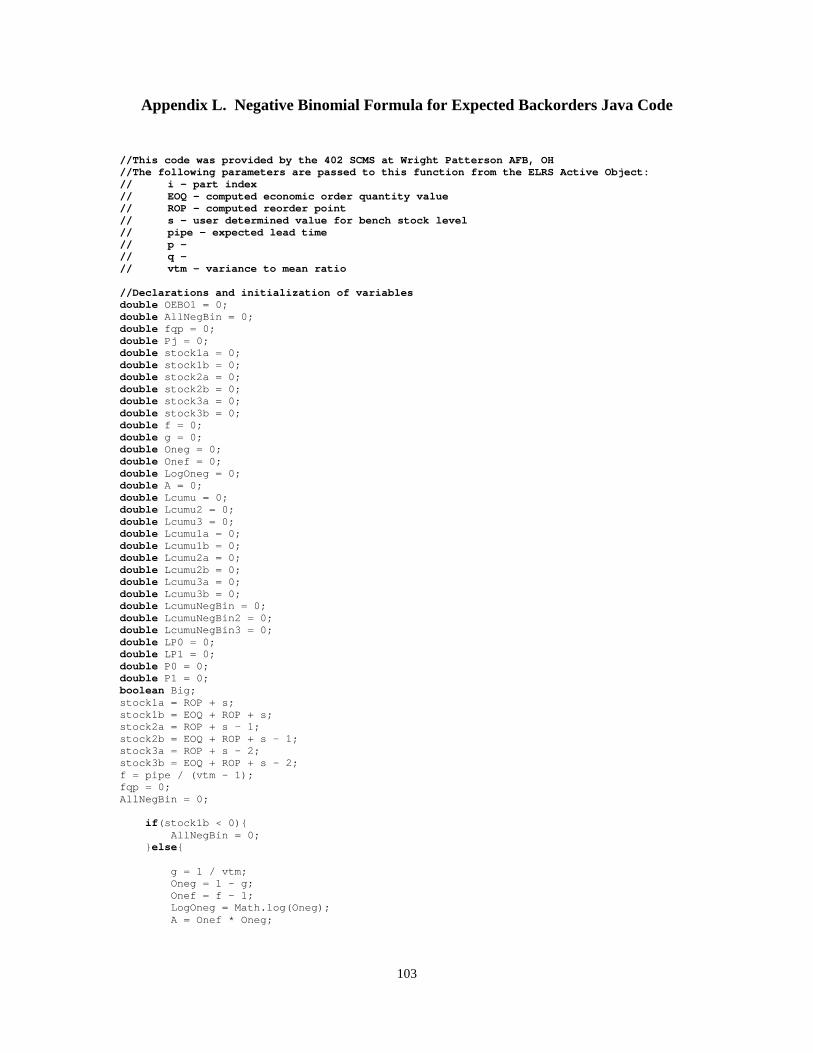
103
Appendix L. Negative Binomial Formula for Expected Backorders Java Code
//This code was provided by the 402 SCMS at Wright Patterson AFB, OH //The following parameters are passed to this function from the ELRS Active Object: // i – part index // EOQ – computed economic order quantity value // ROP – computed reorder point // s – user determined value for bench stock level // pipe – expected lead time // p – // q – // vtm – variance to mean ratio //Declarations and initialization of variables double OEBO1 = 0; double AllNegBin = 0; double fqp = 0; double Pj = 0; double stock1a = 0; double stock1b = 0; double stock2a = 0; double stock2b = 0; double stock3a = 0; double stock3b = 0; double f = 0; double g = 0; double Oneg = 0; double Onef = 0; double LogOneg = 0; double A = 0; double Lcumu = 0; double Lcumu2 = 0; double Lcumu3 = 0; double Lcumu1a = 0; double Lcumu1b = 0; double Lcumu2a = 0; double Lcumu2b = 0; double Lcumu3a = 0; double Lcumu3b = 0; double LcumuNegBin = 0; double LcumuNegBin2 = 0; double LcumuNegBin3 = 0; double LP0 = 0; double LP1 = 0; double P0 = 0; double P1 = 0; boolean Big; stock1a = ROP + s; stock1b = EOQ + ROP + s; stock2a = ROP + s - 1; stock2b = EOQ + ROP + s - 1; stock3a = ROP + s - 2; stock3b = EOQ + ROP + s - 2; f = pipe / (vtm - 1); fqp = 0; AllNegBin = 0; if(stock1b < 0){ AllNegBin = 0; }else{ g = 1 / vtm; Oneg = 1 - g; Onef = f - 1; LogOneg = Math.log(Oneg); A = Onef * Oneg;
104
if(pipe == 0){ if(stock1a < 0){ Lcumu1a = 0; }else{ Lcumu1a = 1; } Lcumu1b = 1; if(stock2b < 0){ Lcumu2a = 0; Lcumu2b = 0; }else if (stock2a < 0) { Lcumu2a = 0; Lcumu2b = 1; }else{ Lcumu2a = 1; Lcumu2b = 1; } if(stock3b < 0){ Lcumu3a = 0; Lcumu3b = 0; }else if (stock3a < 0){ Lcumu3a = 0; Lcumu3b = 1; }else{ Lcumu3a = 1; Lcumu3b = 1; } }else{ P0 = Math.pow(g,f); Lcumu = P0; Lcumu2 = 0; Lcumu3 = 0; LP0 = f * Math.log(g); if(LP0 < -30){ Big = true; }else{ Big = false; } if(stock1a < 0){ Lcumu1a = 0; }else{ Lcumu1a = P0; } Lcumu1b = P0; Lcumu2a = 0; Lcumu2b = 0; Lcumu3a = 0; Lcumu3b = 0; for(int j = 1; j <= stock1b; j++){ if(Big == true){ LP1 = LP0 + Math.log(Onef + j) + LogOneg - Math.log(j); P1 = exp(LP1); Lcumu = Lcumu + P1; Pj = P1 * j; Lcumu2 = Lcumu2 + Pj; Lcumu3 = Lcumu3 + Pj * (j - 1); LP0 = LP1; }else if(Big == false){ P1 = P0 * (A / j + Oneg);

105
Lcumu = Lcumu + P1; Pj = P1 * j; Lcumu2 = Lcumu2 + Pj; Lcumu3 = Lcumu3 + Pj * (j - 1); P0 = P1; } if(j == stock1a){ Lcumu1a = Lcumu; Lcumu2a = Lcumu2; Lcumu3a = Lcumu3; } } Lcumu1b = Lcumu; Lcumu2b = Lcumu2; Lcumu3b = Lcumu3; } fqp = f * q / p; LcumuNegBin = (stock1b * (stock1b + 1) * Lcumu1b) - (stock1a * (stock1a + 1) * Lcumu1a); if(pipe == 0){ LcumuNegBin2 = 0; LcumuNegBin3 = 0; } else { LcumuNegBin2 = 2 * fqp * ((stock2a + 1) * Lcumu2a - (stock2b + 1) * Lcumu2b) / pipe; LcumuNegBin3 = fqp * (fqp + q / p) * (Lcumu3b - Lcumu3a) / pipe / (pipe + vtm - 1); } AllNegBin = LcumuNegBin + LcumuNegBin2 + LcumuNegBin3; } OEBO1 = (0.5 / EOQ) * AllNegBin + fqp - (ROP + s) - 0.5 * (EOQ + 1); return OEBO1;

106
Appendix M. COLT Marginal Analysis Process Java Code
//Declarations double[][] coltMA_Array = new double[2000][18]; //Initialization of COLT Marginal Analysis array for(int a = 0; a <= 1999; a++){ for(int b = 0; b <= 16; b++){ coltMA_Array[a][b] = 0; } } //***************************Create COLT MA Workspace******************************** //Compute Index for(int a = 1, b = 22; a <= wEOQ[0]+2; a++, b++){ coltMA_Array[a-1][0] += a; } //********************Calculate Part 1's COLT MA Parameters*********************** //Compute Part 1 ROP for(int a = -1, b = 22; a <= (wEOQ[0]); a++, b++){ coltMA_Array[a + 1][1] += a; } //Compute Part 1’s EOQ values coltMA_Array[0][2] = 1; coltMA_Array[1][2] = 1; for(int a = 1, b = 22; a <= (wEOQ[0]); a++, b++){ coltMA_Array[a+1][2] = wEOQ[0]; } //Compute Part 1 Level for(int a = 0, b = 22; a <=(wEOQ[0]+1); a++, b++){ coltMA_Array[a][3] = coltMA_Array[a][1] + coltMA_Array[a][2]; } //Compute Part 1 Expected BackOrders (EBOs) for(int a = 0, b = 22; a <= (wEOQ[0]+1); a++, b++){ coltMA_Array[a][4] = calc_nbEBO(0, coltMA_Array[a][2], coltMA_Array[a][1], BenchStock[0], Pipe[0], p[0], q[0], VMR[0]); } //Compute Part 1 Customer Wait Time for(int a = 0, b = 22; a <= (wEOQ[0]+1); a++, b++){ coltMA_Array[a][5] = coltMA_Array[a][4]/get_Main().eLRS.DDR[0]; } //Compute Part 1 EBO Delta for(int a = 0, b = 22; a <= (wEOQ[0]+1); a++, b++){ if(coltMA_Array[a][1] == -1){ coltMA_Array[a][6] = 0; }else if(coltMA_Array[a][1] > -1){ coltMA_Array[a][6] = ((coltMA_Array[a-1][4]-coltMA_Array[a][4])/(coltMA_Array[a][3]-coltMA_Array[a-1][3])); } } //Compute Part 1 Marginal Benefit for(int a = 0, b = 22; a <= (wEOQ[0]+1); a++, b++){ coltMA_Array[a][7] = coltMA_Array[a][6]/get_Main().soS.UnitPrice[0]; } //********************Calculate Part 2's COLT MA Parameters*********************** //Compute Part 2 ROP for(int a = -1, b = 22; a <= (wEOQ[1]); a++, b++){
107
coltMA_Array[a + 1][8] += a; } //Compute Part 2’s EOQ values coltMA_Array[0][9] = 1; coltMA_Array[1][9] = 1; for(int a = 1, b = 22; a <= (wEOQ[1]); a++, b++){ coltMA_Array[a+1][9] = wEOQ[1]; } //Compute Part 2 Level for(int a = 0, b = 22; a <=(wEOQ[1]+1); a++, b++){ coltMA_Array[a][10] = coltMA_Array[a][8] + coltMA_Array[a][9]; } //Compute Part 2 Eexpected BackOrders (EBOs) for(int a = 0, b = 22; a <= (wEOQ[1]+1); a++, b++){ coltMA_Array[a][11] = calc_nbEBO(1, coltMA_Array[a][9], coltMA_Array[a][8], BenchStock[1], Pipe[1], p[1], q[1], VMR[1]); } //Compute Part 2 Customer Wait Time for(int a = 0, b = 22; a <= (wEOQ[1]+1); a++, b++){ coltMA_Array[a][12] = coltMA_Array[a][11]/get_Main().eLRS.DDR[1]; } //Compute Part 2 EBO Delta for(int a = 0, b = 22; a <= (wEOQ[1]+1); a++, b++){ if(coltMA_Array[a][8] == -1){ coltMA_Array[a][13] = 0; }else if(coltMA_Array[a][8] > -1){ coltMA_Array[a][13] = ((coltMA_Array[a-1][11]-coltMA_Array[a][11])/(coltMA_Array[a][10]-coltMA_Array[a-1][10])); } } //Compute Part 2 Marginal Benefit for(int a = 0, b = 22; a <= (wEOQ[1]+1); a++, b++){ coltMA_Array[a][14] = coltMA_Array[a][13]/get_Main().soS.UnitPrice[1]; } //********************Update COLT Sort Value Target*********************** if(wEOQ[0] > wEOQ[1]){ for(int a = 0, b = 22; a <= (wEOQ[0]+1); a++, b++){ coltMA_Array[a][15] = SVTgt; } }else if (wEOQ[0] <= wEOQ[1]){ for(int a = 0, b = 22; a <= (wEOQ[1]+1); a++, b++){ coltMA_Array[a][15] = SVTgt; } } //Initialize ROP variable computed by COLT colt_s[0] = 0; colt_s[1] = 0; //Compute Item to Stock //If Part 1's EOQ is bigger than Part 2's EOQ, Part 1's EOQ + 1 will be used as the stopping //point if(wEOQ[0] > wEOQ[1]){ //Loop through the arrays to run the marginal analysis //array1 initializes the array containing Part 1's information //array2 initializes the array containing Part 2's information //array3 initializes the array containing the Sort Value Target //All of the above arrays are created in order to output a Marginal Analysis table to //Excel
108
for(int a = 0, array1 = 1, array2 = 1, array3 = 1, row = 23; a <= (wEOQ[0] + 1); a++){ //If the marginal benefit of Part 1 and the marginal benefit of Part 2 are both bigger //than the Sort Value Target run this part of the if-else statement if((coltMA_Array[array1][7] > coltMA_Array[array3][15]) && (coltMA_Array[array2][14] > coltMA_Array[array3][15])){ //If the marginal benefit of Part 1 is bigger when compared to the //marginal benefit of //Part 2, increase the ROP of Part 1 by a value of 1 and then move to the next marginal //benefit value of Part 1 if((coltMA_Array[array1][7] > coltMA_Array[array2][14])){ coltMA_Array[array3][16] = 1; array1++; array3++; row++; colt_s[0]++; //If the marginal benefit of Part 2 is bigger when compared to the marginal benefit of //Part 1, increase the ROP of Part 2 by a value of 1 and then move to the next marginal //benefit value of Part 2 }else if((coltMA_Array[array1][7] < coltMA_Array[array2][14])){ coltMA_Array[array3][16] = 2; array2++; array3++; row++; colt_s[1]++; } //If only the marginal benefit of Part 1 is bigger than the Sort Value Target run this //part of the if-else statement }else if((coltMA_Array[array1][7] > coltMA_Array[array3][15]) && (coltMA_Array[array2][14] < coltMA_Array[array3][15])){ coltMA_Array[array3][16] = 1; array1++; array3++; row++; colt_s[0]++; //If only the marginal benefit of Part 2 is bigger than the Sort Value Target run this //part of the if-else statement }else if((coltMA_Array[array1][7] < coltMA_Array[array3][15]) && (coltMA_Array[array2][14] > coltMA_Array[array3][15])){ coltMA_Array[array3][16] = 2; array2++; array3++; row++; colt_s[1]++; } } //If Part 2's EOQ is bigger than Part 1's EOQ, Part 2's EOQ + 1 will be used as the //stopping point }else if(wEOQ[0] < wEOQ[1]){ //Loop through the arrays to run the marginal analysis //array1 initializes the array containing Part 1's information //array2 initializes the array containing Part 2's information //array3 initializes the array containing the Sort Value Target //All of the above arrays are created in order to output a Marginal Analysis table to //Excel for(int a = 0, array1 = 1, array2 = 1, array3 = 1, row = 23; a <= (wEOQ[1] + 1); a++){ //If the marginal benefit of Part 1 and the marginal benefit of Part 2 are both bigger //than the Sort Value Target run this part of the if-else statement if((coltMA_Array[array1][7] > coltMA_Array[array3][15]) && (coltMA_Array[array2][14] > coltMA_Array[array3][15])){ //If the marginal benefit of Part 1 is bigger when compared to the marginal benefit of //Part 2, increase the ROP of Part 1 by a value of 1and then move to the next marginal //benefit value of Part 1 if((coltMA_Array[array1][7] > coltMA_Array[array2][14])){ coltMA_Array[array3][16] = 1; array1++; array3++; row++;
109
colt_s[0]++; //If the marginal benefit of Part 2 is bigger when compared to the marginal benefit of //Part 1, increase the ROP of Part 2 by a value of 1 and then move to the next marginal //benefit value of Part 2 }else if((coltMA_Array[array1][7] < coltMA_Array[array2][14])){ coltMA_Array[array3][16] = 2; array2++; array3++; row++; colt_s[1]++; } //If only the marginal benefit of Part 1 is bigger than the Sort Value Target run this //part of the if-else statement }else if((coltMA_Array[array1][7] > coltMA_Array[array3][15]) && (coltMA_Array[array2][14] < coltMA_Array[array3][15])){ coltMA_Array[array3][16] = 1; array1++; array3++; row++; colt_s[0]++; //If only the marginal benefit of Part 2 is bigger than the Sort Value Target run this //part of the if-else statement }else if((coltMA_Array[array1][7] < coltMA_Array[array3][15]) && (coltMA_Array[array2][14] > coltMA_Array[array3][15])){ coltMA_Array[array3][16] = 2; array2++; array3++; row++; colt_s[1]++; } } //If Part 2's EOQ equal to Part 1's EOQ, Part 2's EOQ + 1 will be used as the stopping //point }else if(wEOQ[0] == wEOQ[1]){ //Loop through the arrays to run the marginal analysis //array1 initializes the array containing Part 1's information //array2 initializes the array containing Part 2's information //array3 initializes the array containing the Sort Value Target //All of the above arrays are created in order to output a Marginal Analysis table to //Excel for(int a = 0, array1 = 1, array2 = 1, array3 = 1, row = 23; a <= (wEOQ[1] + 1); a++){ //If the marginal benefit of Part 1 and the marginal benefit of Part 2 are both bigger than the Sort Value Target run this part of the if-else statement if((coltMA_Array[array1][7] > coltMA_Array[array3][15]) && (coltMA_Array[array2][14] > coltMA_Array[array3][15])){ //If the marginal benefit of Part 1 is bigger when compared to the marginal benefit of //Part 2, increase the ROP of Part 1 by a value of 1 and then move to the next marginal //benefit value of Part 1 if((coltMA_Array[array1][7] > coltMA_Array[array2][14])){ coltMA_Array[array3][16] = 1; array1++; array3++; row++; colt_s[0]++; //If the marginal benefit of Part 2 is bigger when compared to the marginal benefit of //Part 1, increase the ROP of Part 2 by a value of 1 and then move to the next marginal //benefit value of Part 2
}else if((coltMA_Array[array1][7] < coltMA_Array[array2][14])){
coltMA_Array[array3][16] = 2; array2++; array3++; row++; colt_s[1]++; } //If only the marginal benefit of Part 1 is bigger than the Sort Value Target run this //part of the if-else statement
110
}else if((coltMA_Array[array1][7] > coltMA_Array[array3][15]) && (coltMA_Array[array2][14] < coltMA_Array[array3][15])){ coltMA_Array[array3][16] = 1; array1++; array3++; row++; colt_s[0]++; //If only the marginal benefit of Part 2 is bigger than the Sort Value Target run this //part of the if-else statement }else if((coltMA_Array[array1][7] < coltMA_Array[array3][15]) && (coltMA_Array[array2][14] > coltMA_Array[array3][15])){ coltMA_Array[array3][16] = 2; array2++; array3++; row++; colt_s[1]++; } } }
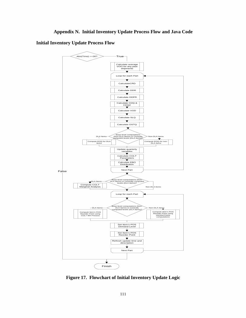
111
Appendix N. Initial Inventory Update Process Flow and Java Code
Initial Inventory Update Process Flow
Abs(Time) ==30?
Finish
False
True
Calculate DDR
Calculate DDFR
Calculate SLQ
Calculate COLT Parameters
Calculate EBO Distribution
Compute COLT Marginal Analysis
Set Item’s POS Demand Level
Set Item’s POS Reorder Point
Compute Item’s POS Reorder Point using COLT MA Process
Compute Item’s POS Reorder Point using
standard base computations
Base-level computations (Non-DLA Items) or Centrally
computed levels (DLA Items)?
Refresh update time and description
Non-DLA ItemsDLA Items
Calculate average VOO for any past
shipments
Update quarterly variables
Calculate OSTQ
Loop for each Part
Next Part
Calculate VOD
Base-level computations (Non-DLA Items) or Centrally computed levels (DLA Items)?
Compute EOQ for non-DLA items
Compute EOQ for DLA items
Non-DLA ItemsDLA Items
Next Part
Loop for each Part
Base-level computations (Non-DLA Items) or Centrally computed
levels (DLA Items)?DLA Items
Non-DLA Items
CalculateCRD
Calculate CDQ & CDQ2
Figure 17. Flowchart of Initial Inventory Update Logic
112
Initial Inventory Update Process Java Code //Calculate average Variance of Order and Ship Time (VOO) for any past shipments of Part 1 if(p0VOO.size() != 0){ double sump0VOO = 0; for (int j = 0; j < p0VOO.size(); j++){ sump0VOO += p0VOO.get(j); } qtrlyVOO[0] = sump0VOO/p0VOO.size(); }else if(p0VOO.size() == 0){ qtrlyVOO[0] = 0; } //Calculate average Variance of Order and Ship Time (VOO) for any past shipments of Part 2 if(p1VOO.size() != 0){ double sump1VOO = 0; for (int j = 0; j < p1VOO.size(); j++){ sump1VOO += p1VOO.get(j); } qtrlyVOO[1] = sump1VOO/p1VOO.size(); }else if(p1VOO.size() == 0){ qtrlyVOO[1] = 0; } //Clear VOO arrays p0VOO.clear(); p1VOO.clear(); //Calculate inventory management parameters for each part for(int i = 0; i <= 1; i++){ //Calculate Daily Demand Rate calcCRD(0,i);
//Calculate Daily Demand Rate
calcDDR(i); //Calculate Daily Demand Frequency Rate calcDDFR(i); //Calculate Daily Demand Rate calcCDQ_CDQ2(0,i); //Calculate Variance Of Demand calcVOD(i); //Calculate Safety Level Quantity calcSLQ(i); sLQ_formula[i] = sLQ_formulatempvalue[i]; //Calculate Order and Ship Time Quantity calcOSTQ(i); //Update EOQ Value based on how inventory calculations are computed: Base v. Centrally if(Simulation.SLQ_Calculation == 0){ Base_EOQ(i); }else if (Simulation.SLQ_Calculation == 1){ DLA_EOQ(i); } //Calculate COLT parameters calcCOLTParameters(i); //Calculate EBO Distribution
113
EBO[i] = calc_nbEBO(i, wEOQ[i], s[i], BenchStock[i], Pipe[i], p[i], q[i], VMR[i]); } //Compute COLT Marginal Analysis if(Simulation.SLQ_Calculation == 1){ calcCOLTMA(); } for(int i = 0; i <= 1; i++){ //Compute Primary Operating Stock Consumable Item Reorder Point calcROP(i); //Compute Primary Operating Stock Consumable Item Demand Level calcEOQDL(i); //Set Primary Operating Stock Consumable Item Demand Level S[i] = EOQ_DL[i]; //Set Primary Operating Stock Consumable Item Reorder Point s[i] = ROP[i]; //Update refresh time and description updatePeriod[i] = "Initial"; updateDate[i] = time(); }
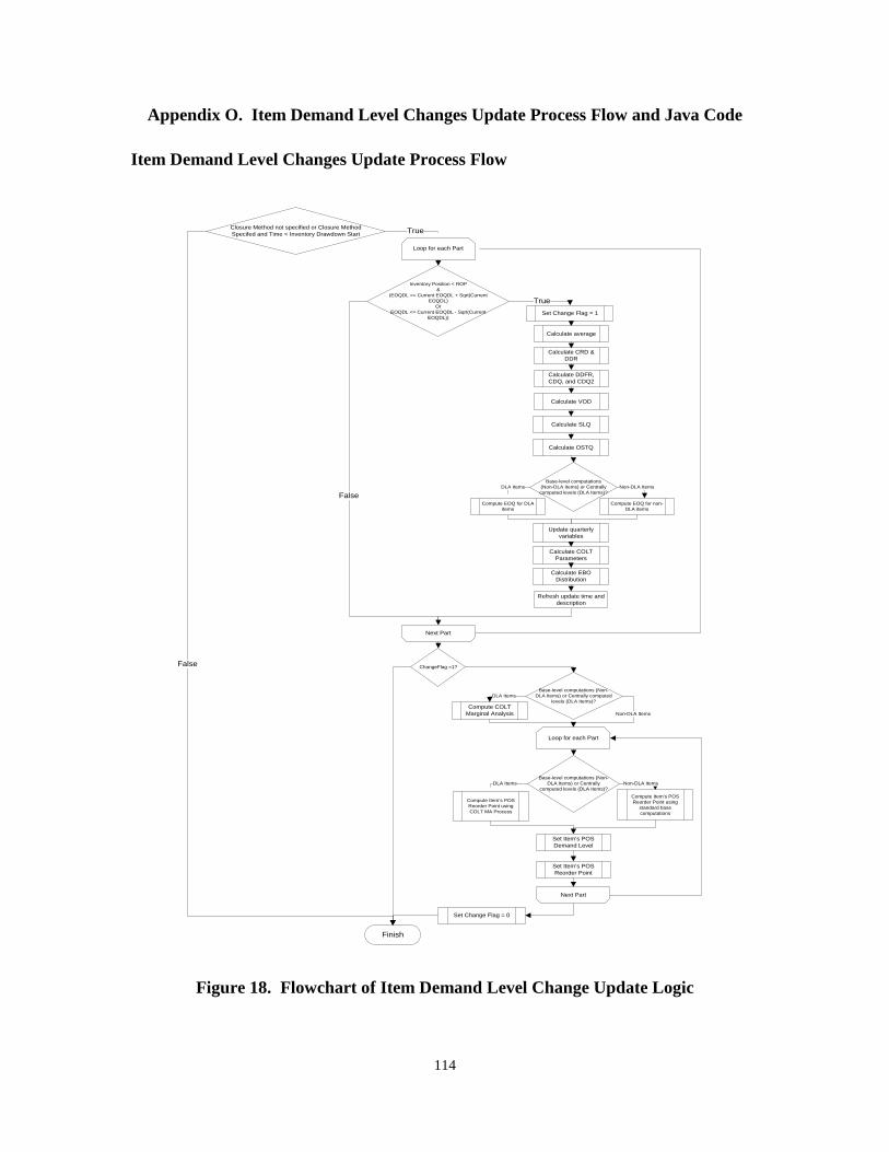
114
Appendix O. Item Demand Level Changes Update Process Flow and Java Code
Item Demand Level Changes Update Process Flow
Closure Method not specified or Closure Method Specifed and Time < Inventory Drawdown Start
Finish
False
True
Loop for each Part
Inventory Position < ROP&
(EOQDL >= Current EOQDL + Sqrt(Current EOQDL)
OrEOQDL <= Current EOQDL - Sqrt(Current
EOQDL))
True
False
Calculate CRD & DDR
Calculate DDFR, CDQ, and CDQ2
Calculate SLQ
Calculate COLT Parameters
Calculate EBO Distribution
Compute COLT Marginal Analysis
Set Item’s POS Demand Level
Set Item’s POS Reorder Point
Compute Item’s POS Reorder Point using COLT MA Process
Compute Item’s POS Reorder Point using
standard base computations
Base-level computations (Non-DLA Items) or Centrally
computed levels (DLA Items)?Non-DLA ItemsDLA Items
Calculate average
Update quarterly variables
Calculate OSTQ
Next Part
Calculate VOD
Base-level computations (Non-DLA Items) or Centrally computed levels (DLA Items)?
Compute EOQ for non-DLA items
Compute EOQ for DLA items
Non-DLA ItemsDLA Items
Next Part
Loop for each Part
Base-level computations (Non-DLA Items) or Centrally computed
levels (DLA Items)?DLA Items
Non-DLA Items
Set Change Flag = 1
ChangeFlag =1?
Refresh update time and description
Set Change Flag = 0
Figure 18. Flowchart of Item Demand Level Change Update Logic
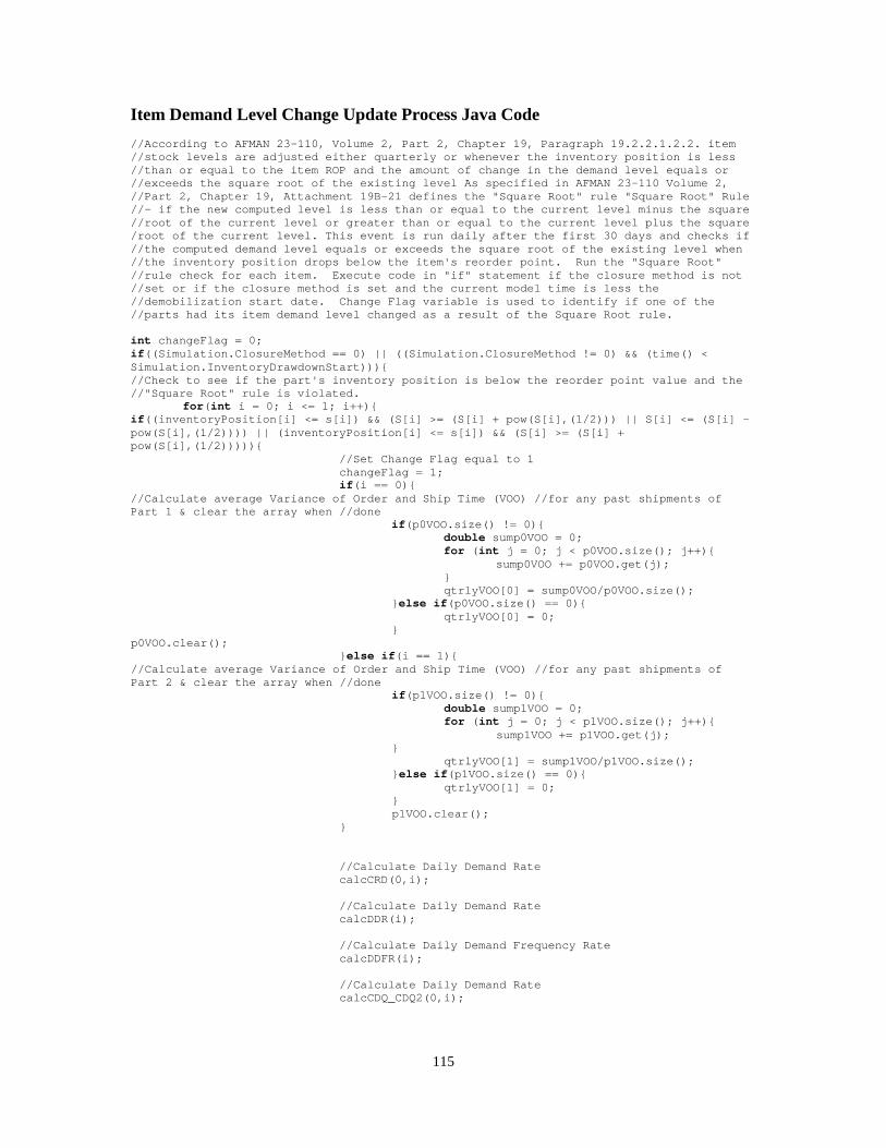
115
Item Demand Level Change Update Process Java Code
//According to AFMAN 23-110, Volume 2, Part 2, Chapter 19, Paragraph 19.2.2.1.2.2. item //stock levels are adjusted either quarterly or whenever the inventory position is less //than or equal to the item ROP and the amount of change in the demand level equals or //exceeds the square root of the existing level As specified in AFMAN 23-110 Volume 2, //Part 2, Chapter 19, Attachment 19B-21 defines the "Square Root" rule "Square Root" Rule //- if the new computed level is less than or equal to the current level minus the square //root of the current level or greater than or equal to the current level plus the square /root of the current level. This event is run daily after the first 30 days and checks if //the computed demand level equals or exceeds the square root of the existing level when //the inventory position drops below the item's reorder point. Run the "Square Root" //rule check for each item. Execute code in "if" statement if the closure method is not //set or if the closure method is set and the current model time is less the //demobilization start date. Change Flag variable is used to identify if one of the //parts had its item demand level changed as a result of the Square Root rule. int changeFlag = 0; if((Simulation.ClosureMethod == 0) || ((Simulation.ClosureMethod != 0) && (time() < Simulation.InventoryDrawdownStart))){ //Check to see if the part's inventory position is below the reorder point value and the //"Square Root" rule is violated. for(int i = 0; i <= 1; i++){ if((inventoryPosition[i] <= s[i]) && (S[i] >= (S[i] + pow(S[i],(1/2))) || S[i] <= (S[i] - pow(S[i],(1/2)))) || (inventoryPosition[i] <= s[i]) && (S[i] >= (S[i] + pow(S[i],(1/2))))){ //Set Change Flag equal to 1 changeFlag = 1; if(i == 0){ //Calculate average Variance of Order and Ship Time (VOO) //for any past shipments of Part 1 & clear the array when //done if(p0VOO.size() != 0){ double sump0VOO = 0; for (int j = 0; j < p0VOO.size(); j++){ sump0VOO += p0VOO.get(j); } qtrlyVOO[0] = sump0VOO/p0VOO.size(); }else if(p0VOO.size() == 0){ qtrlyVOO[0] = 0; } p0VOO.clear(); }else if(i == 1){ //Calculate average Variance of Order and Ship Time (VOO) //for any past shipments of Part 2 & clear the array when //done if(p1VOO.size() != 0){ double sump1VOO = 0; for (int j = 0; j < p1VOO.size(); j++){ sump1VOO += p1VOO.get(j); } qtrlyVOO[1] = sump1VOO/p1VOO.size(); }else if(p1VOO.size() == 0){ qtrlyVOO[1] = 0; } p1VOO.clear(); } //Calculate Daily Demand Rate calcCRD(0,i);
//Calculate Daily Demand Rate calcDDR(i); //Calculate Daily Demand Frequency Rate calcDDFR(i); //Calculate Daily Demand Rate calcCDQ_CDQ2(0,i);
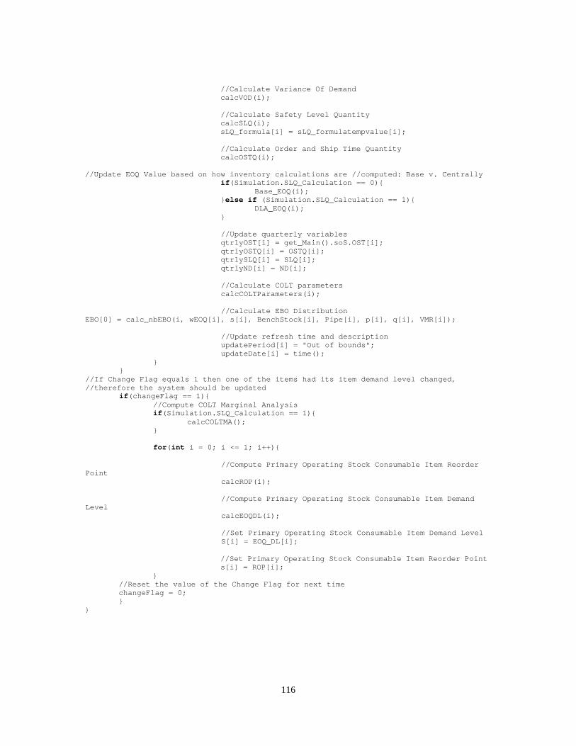
116
//Calculate Variance Of Demand calcVOD(i); //Calculate Safety Level Quantity calcSLQ(i); sLQ_formula[i] = sLQ_formulatempvalue[i]; //Calculate Order and Ship Time Quantity calcOSTQ(i); //Update EOQ Value based on how inventory calculations are //computed: Base v. Centrally if(Simulation.SLQ_Calculation == 0){ Base_EOQ(i); }else if (Simulation.SLQ_Calculation == 1){ DLA_EOQ(i); } //Update quarterly variables qtrlyOST[i] = get_Main().soS.OST[i]; qtrlyOSTQ[i] = OSTQ[i]; qtrlySLQ[i] = SLQ[i]; qtrlyND[i] = ND[i]; //Calculate COLT parameters calcCOLTParameters(i); //Calculate EBO Distribution EBO[0] = calc_nbEBO(i, wEOQ[i], s[i], BenchStock[i], Pipe[i], p[i], q[i], VMR[i]); //Update refresh time and description updatePeriod[i] = "Out of bounds"; updateDate[i] = time(); } } //If Change Flag equals 1 then one of the items had its item demand level changed, //therefore the system should be updated if(changeFlag == 1){ //Compute COLT Marginal Analysis if(Simulation.SLQ_Calculation == 1){ calcCOLTMA(); } for(int i = 0; i <= 1; i++){ //Compute Primary Operating Stock Consumable Item Reorder Point calcROP(i); //Compute Primary Operating Stock Consumable Item Demand Level calcEOQDL(i); //Set Primary Operating Stock Consumable Item Demand Level S[i] = EOQ_DL[i]; //Set Primary Operating Stock Consumable Item Reorder Point s[i] = ROP[i]; } //Reset the value of the Change Flag for next time changeFlag = 0; } }
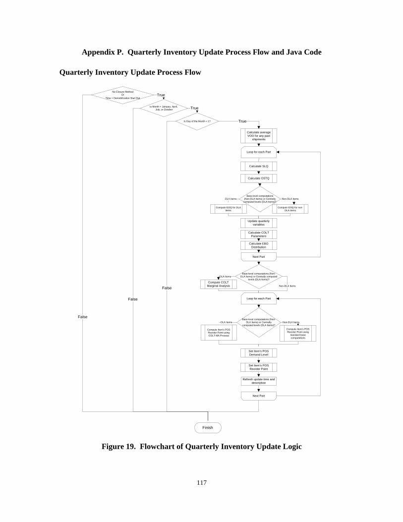
117
Appendix P. Quarterly Inventory Update Process Flow and Java Code
Quarterly Inventory Update Process Flow
No Closure MethodOr
Time < Demobilization Start Dat
Calculate SLQ
Calculate COLT Parameters
Calculate EBO Distribution
Compute COLT Marginal Analysis
Set Item’s POS Demand Level
Set Item’s POS Reorder Point
Compute Item’s POS Reorder Point using COLT MA Process
Compute Item’s POS Reorder Point using
standard base computations
Base-level computations (Non-DLA Items) or Centrally
computed levels (DLA Items)?
Refresh update time and description
Finish
Non-DLA ItemsDLA Items
False
Calculate average VOO for any past
shipments
True
Update quarterly variables
Calculate OSTQ
Loop for each Part
Next Part
Is Month = January, April, July, or October
True
False
Is Day of the Month = 1? True
False
Base-level computations (Non-DLA Items) or Centrally computed levels (DLA Items)?
Compute EOQ for non-DLA items
Compute EOQ for DLA items
Non-DLA ItemsDLA Items
Next Part
Loop for each Part
Base-level computations (Non-DLA Items) or Centrally computed
levels (DLA Items)?DLA Items
Non-DLA Items
Figure 19. Flowchart of Quarterly Inventory Update Logic

118
Quarterly Inventory Update Process Java Code
//Execute code in "if" statement if the closure method is not set or if the closure method is set //and the current model time is less the demobilization //start date if((Simulation.ClosureMethod == 0) || ((Simulation.ClosureMethod != 0) && (time() < Simulation.RedeploymentStart))){ //Is simulated month equal January, April, July or October? if(getMonth() == 0 || getMonth() == 3 || getMonth() == 6 || getMonth() == 9){ //Is simulated calendar day equal to 1? if(getDayOfMonth() == 1){ //Calculate average Variance of Order and Ship Time (VOO) for any past //shipments of Part 1 if(p0VOO.size() != 0){ double sump0VOO = 0; for (int j = 0; j < p0VOO.size(); j++){ sump0VOO += p0VOO.get(j); } qtrlyVOO[0] = sump0VOO/p0VOO.size(); }else if(p0VOO.size() == 0){ qtrlyVOO[0] = 0; } //Calculate average VOO for any past shipments of Part 2 if(p1VOO.size() != 0){ double sump1VOO = 0; for (int j = 0; j < p1VOO.size(); j++){ sump1VOO += p1VOO.get(j); } qtrlyVOO[1] = sump1VOO/p1VOO.size(); }else if(p1VOO.size() == 0){ qtrlyVOO[1] = 0; } //Clear VOO arrays p0VOO.clear(); p1VOO.clear(); for(int i = 0; i <= 1; i++){ //Calculate Safety Level Quantity calcSLQ(i); sLQ_formula[i] = sLQ_formulatempvalue[i];
//Calculate Order and Ship Time Quantity calcOSTQ(i);
//Update EOQ Value based on how inventory calculations are //computed: Base v. Centrally
if(Simulation.SLQ_Calculation == 0){ Base_EOQ(i); }else if (Simulation.SLQ_Calculation == 1){ DLA_EOQ(i); } //Calculate COLT parameters calcCOLTParameters(i); //Calculate EBO Distribution
EBO[i] = calc_nbEBO(i, wEOQ[i], s[i], BenchStock[i], Pipe[i], p[i], q[i], VMR[i]);
}
//Compute COLT Marginal Analysis if inventory calculations are centrally computed
if(Simulation.SLQ_Calculation == 1){ calcCOLTMA();
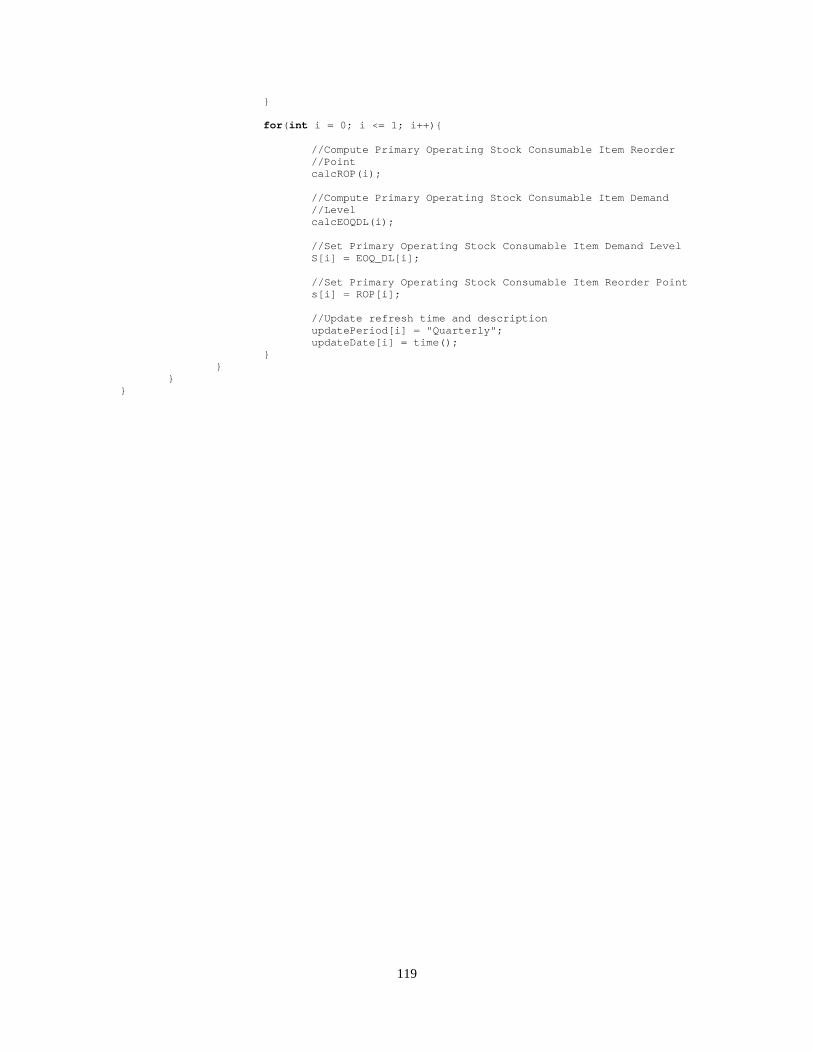
119
} for(int i = 0; i <= 1; i++){
//Compute Primary Operating Stock Consumable Item Reorder //Point
calcROP(i);
//Compute Primary Operating Stock Consumable Item Demand //Level
calcEOQDL(i); //Set Primary Operating Stock Consumable Item Demand Level S[i] = EOQ_DL[i]; //Set Primary Operating Stock Consumable Item Reorder Point s[i] = ROP[i]; //Update refresh time and description updatePeriod[i] = "Quarterly"; updateDate[i] = time(); } } } }
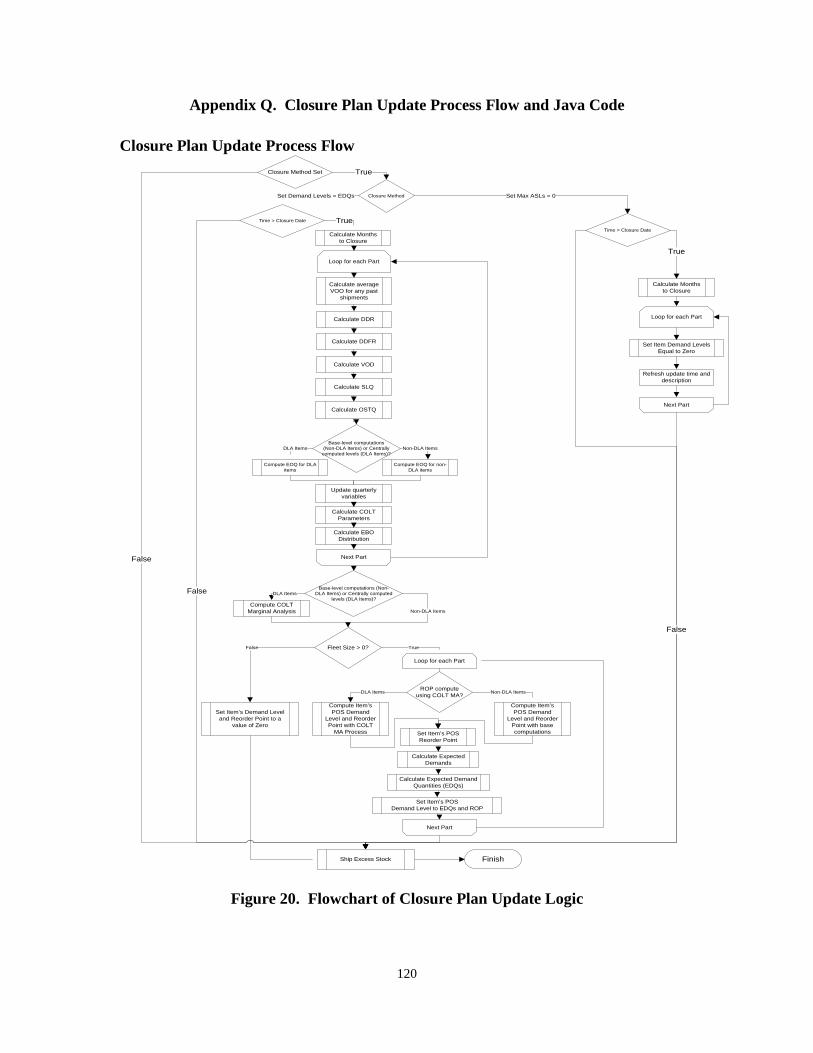
120
Appendix Q. Closure Plan Update Process Flow and Java Code
Closure Plan Update Process Flow Closure Method Set
Set Item Demand Levels Equal to Zero
Refresh update time and description
Finish
False
Calculate Months to Closure
Set Max ASLs = 0
Loop for each Part
Next Part
Closure Method
True
Set Demand Levels = EDQs
Time > Closure Date
True
Time > Closure Date
Calculate Months to Closure
Set Item’s POS Reorder Point
Calculate Expected Demands
Compute Item’s POS Demand
Level and Reorder Point with COLT
MA Process
ROP compute using COLT MA?
Calculate Expected Demand Quantities (EDQs)
Set Item’s POS Demand Level to EDQs and ROP
False
Next Part
False
True
Calculate DDR
Calculate DDFR
Calculate SLQ
Calculate COLT Parameters
Calculate EBO Distribution
Compute COLT Marginal Analysis
Calculate average VOO for any past
shipments
Update quarterly variables
Calculate OSTQ
Loop for each Part
Calculate VOD
Base-level computations (Non-DLA Items) or Centrally computed levels (DLA Items)?
Compute EOQ for non-DLA items
Compute EOQ for DLA items
Non-DLA ItemsDLA Items
Next Part
Base-level computations (Non-DLA Items) or Centrally computed
levels (DLA Items)?
Loop for each Part
DLA Items
Non-DLA Items
Fleet Size > 0?
DLA Items Non-DLA Items
True
Set Item’s Demand Level and Reorder Point to a
value of Zero
Compute Item’s POS Demand
Level and Reorder Point with base computations
False
Ship Excess Stock
Figure 20. Flowchart of Closure Plan Update Logic

121
Closure Plan Update Process Java Code //Execute the first part of this if-else statement if closure method is to set Maximum Adjusted //Stock levels to zero if(Simulation.ClosureMethod == 1){ //Calculate Months to Closure ClosureMonth = getMonth(timeToDate(getEngine().getStopTime())); ClosureYear = getYear(timeToDate(getEngine().getStopTime())); StartMonth = getMonth(timeToDate(Simulation.RedeploymentStart)); StartYear = getYear(timeToDate(Simulation.RedeploymentStart)); if(ClosureYear == getYear()){ MToC = ClosureMonth - getMonth(); }else if(ClosureYear > getYear() && ClosureMonth == getMonth()){ MToC = 12 * (ClosureYear-getYear()); }else if(ClosureYear > getYear() && ClosureMonth > getMonth()){ MToC = 12*(ClosureYear - getYear()) + (ClosureMonth - getMonth()); }else if(ClosureYear > getYear() && ClosureMonth < getMonth()){ MToC = 12*(ClosureYear - getYear()) - (getMonth()- ClosureMonth); } //Set stock levels to 0 and refresh update time and description for(int i = 0; i <= 1; i++){ S[i] = 0; s[i] = 0; updatePeriod[i] = "Closure - Max ASLs = 0"; updateDate[i] = time(); } //Execute the second part of this if-else statement if closure method is to utilized //Expected Demand Quantities as the item's new Demand Level }else if(Simulation.ClosureMethod == 2){ //Calculate Months to Closure ClosureMonth = getMonth(timeToDate(getEngine().getStopTime())); ClosureYear = getYear(timeToDate(getEngine().getStopTime())); StartMonth = getMonth(timeToDate(Simulation.RedeploymentStart)); StartYear = getYear(timeToDate(Simulation.RedeploymentStart)); if(ClosureYear == getYear()){ MToC = ClosureMonth - getMonth(); }else if(ClosureYear > getYear() && ClosureMonth == getMonth()){ MToC = 12 * (ClosureYear-getYear()); }else if(ClosureYear > getYear() && ClosureMonth > getMonth()){ MToC = 12*(ClosureYear - getYear()) + (ClosureMonth - getMonth()); }else if(ClosureYear > getYear() && ClosureMonth < getMonth()){ MToC = 12*(ClosureYear - getYear()) - (getMonth()- ClosureMonth); } for(int i = 0; i <= 1; i++){ if(i == 0){
//Calculate average Variance of Order and Ship Time (VOO) for any //past shipments of Part 1
if(p0VOO.size() != 0){ double sump0VOO = 0; for (int j = 0; j < p0VOO.size(); j++){ sump0VOO += p0VOO.get(j); } qtrlyVOO[0] = sump0VOO/p0VOO.size(); }else if(p0VOO.size() == 0){ qtrlyVOO[0] = 0; } //Clear VOO arrays p0VOO.clear(); }else if(i == 1){ //Calculate average VOO for any past shipments of Part 2
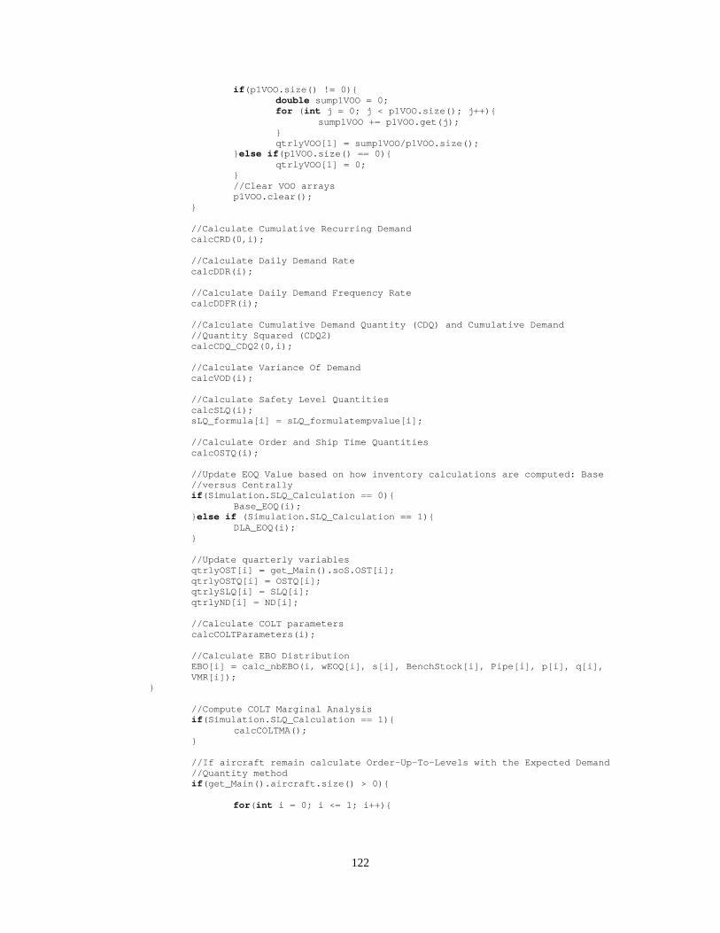
122
if(p1VOO.size() != 0){ double sump1VOO = 0; for (int j = 0; j < p1VOO.size(); j++){ sump1VOO += p1VOO.get(j); } qtrlyVOO[1] = sump1VOO/p1VOO.size(); }else if(p1VOO.size() == 0){ qtrlyVOO[1] = 0; } //Clear VOO arrays p1VOO.clear(); } //Calculate Cumulative Recurring Demand calcCRD(0,i);
//Calculate Daily Demand Rate calcDDR(i); //Calculate Daily Demand Frequency Rate calcDDFR(i);
//Calculate Cumulative Demand Quantity (CDQ) and Cumulative Demand //Quantity Squared (CDQ2)
calcCDQ_CDQ2(0,i); //Calculate Variance Of Demand calcVOD(i); //Calculate Safety Level Quantities calcSLQ(i); sLQ_formula[i] = sLQ_formulatempvalue[i]; //Calculate Order and Ship Time Quantities calcOSTQ(i);
//Update EOQ Value based on how inventory calculations are computed: Base //versus Centrally
if(Simulation.SLQ_Calculation == 0){ Base_EOQ(i); }else if (Simulation.SLQ_Calculation == 1){ DLA_EOQ(i); } //Update quarterly variables qtrlyOST[i] = get_Main().soS.OST[i]; qtrlyOSTQ[i] = OSTQ[i]; qtrlySLQ[i] = SLQ[i]; qtrlyND[i] = ND[i]; //Calculate COLT parameters calcCOLTParameters(i); //Calculate EBO Distribution
EBO[i] = calc_nbEBO(i, wEOQ[i], s[i], BenchStock[i], Pipe[i], p[i], q[i], VMR[i]);
} //Compute COLT Marginal Analysis if(Simulation.SLQ_Calculation == 1){ calcCOLTMA(); }
//If aircraft remain calculate Order-Up-To-Levels with the Expected Demand //Quantity method
if(get_Main().aircraft.size() > 0){ for(int i = 0; i <= 1; i++){
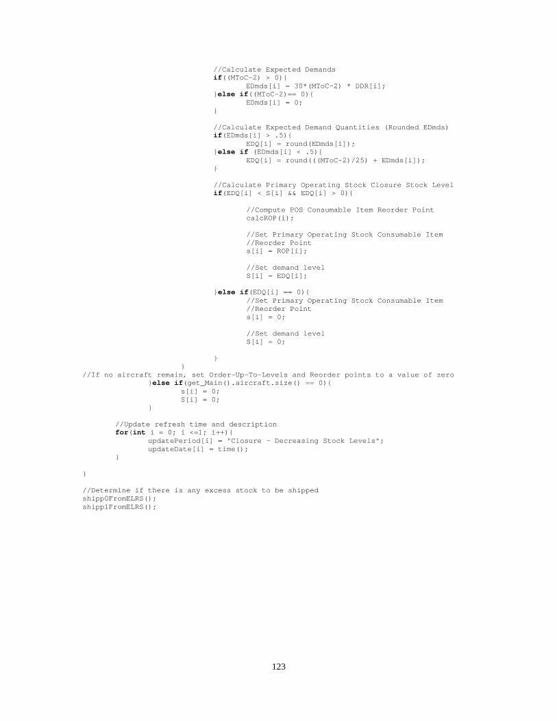
123
//Calculate Expected Demands if((MToC-2) > 0){ EDmds[i] = 30*(MToC-2) * DDR[i]; }else if((MToC-2)== 0){ EDmds[i] = 0; } //Calculate Expected Demand Quantities (Rounded EDmds) if(EDmds[i] > .5){ EDQ[i] = round(EDmds[i]); }else if (EDmds[i] < .5){ EDQ[i] = round(((MToC-2)/25) + EDmds[i]); } //Calculate Primary Operating Stock Closure Stock Level if(EDQ[i] < S[i] && EDQ[i] > 0){
//Compute POS Consumable Item Reorder Point calcROP(i); //Set Primary Operating Stock Consumable Item //Reorder Point
s[i] = ROP[i]; //Set demand level
S[i] = EDQ[i];
}else if(EDQ[i] == 0){ //Set Primary Operating Stock Consumable Item //Reorder Point
s[i] = 0; //Set demand level
S[i] = 0; } } //If no aircraft remain, set Order-Up-To-Levels and Reorder points to a value of zero }else if(get_Main().aircraft.size() == 0){ s[i] = 0; S[i] = 0; } //Update refresh time and description for(int i = 0; i <=1; i++){ updatePeriod[i] = "Closure - Decreasing Stock Levels"; updateDate[i] = time(); } } //Determine if there is any excess stock to be shipped shipp0FromELRS(); shipp1FromELRS();
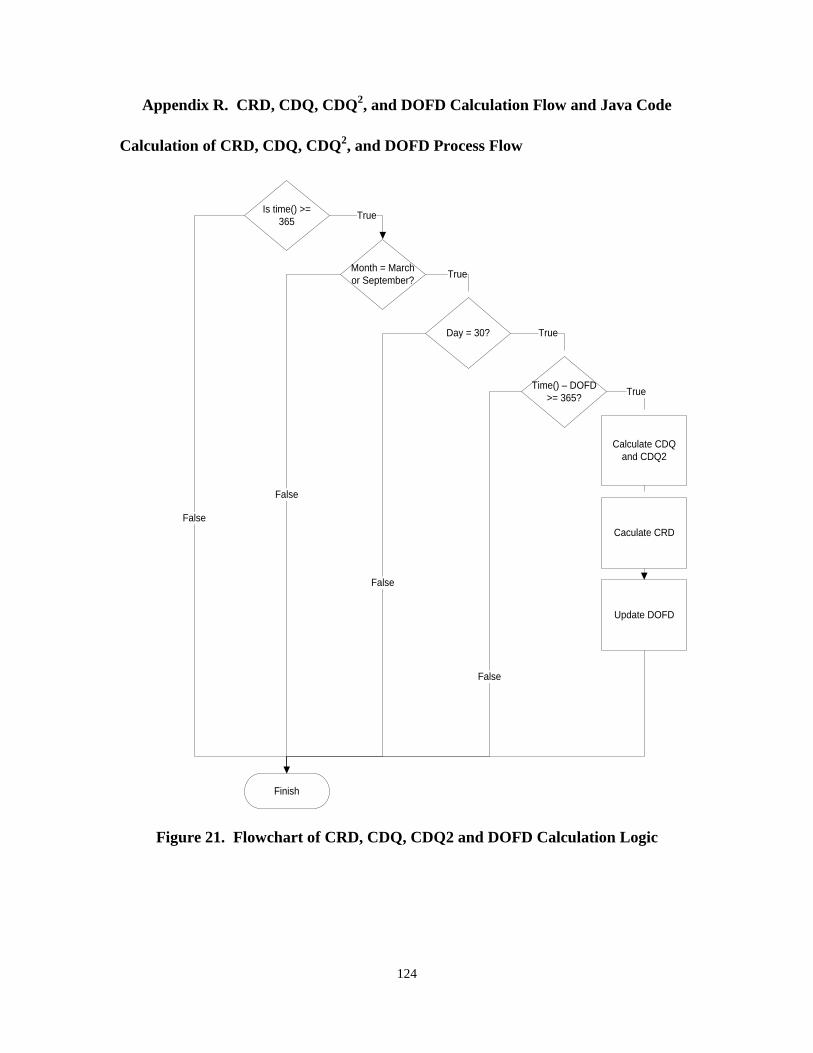
124
Appendix R. CRD, CDQ, CDQ2, and DOFD Calculation Flow and Java Code
Calculation of CRD, CDQ, CDQ2, and DOFD Process Flow
Is time() >= 365
Month = March or September?
Day = 30?
Calculate CDQ and CDQ2
Time() – DOFD >= 365?
True
False
True
True
True
Finish
False
False
False
Caculate CRD
Update DOFD
Figure 21. Flowchart of CRD, CDQ, CDQ2 and DOFD Calculation Logic
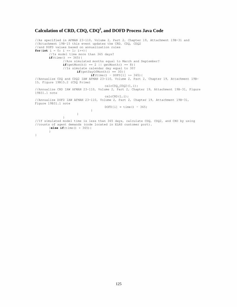
125
Calculation of CRD, CDQ, CDQ2, and DOFD Process Java Code //As specified in AFMAN 23-110, Volume 2, Part 2, Chapter 19, Attachment 19B-31 and //Attachment 19B-15 this event updates the CRD, CDQ, CDQ2 //and DOFD values based on annualization rules for(int i = 0; i <= 1; i++){ //Is model time more than 365 days? if(time() >= 365){ //Are simulated months equal to March and September? if(getMonth() == 2 || getMonth() == 8){ //Is simulate calendar day equal to 30? if(getDayOfMonth() == 30){ if(time() - DOFD[i] >= 365){ //Annualize CDQ and CDQ2 IAW AFMAN 23-110, Volume 2, Part 2, Chapter 19, Attachment 19B-15, Figure 19B15.2 (CDQ Prime) calcCDQ_CDQ2(1,i); //Annualize CRD IAW AFMAN 23-110, Volume 2, Part 2, Chapter 19, Attachment 19B-31, Figure 19B31.1 note calcCRD(1,i); //Annualize DOFD IAW AFMAN 23-110, Volume 2, Part 2, Chapter 19, Attachment 19B-31, Figure 19B31.1 note DOFD[i] = time() - 365; } } } //If simulated model time is less than 365 days, calculate CDQ, CDQ2, and CRD by using //counts of agent demands (code located in ELRS customer port). }else if(time() < 365){ } }
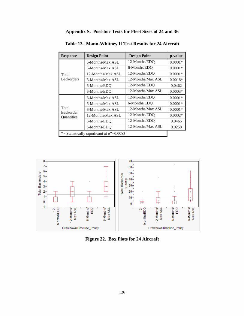
126
Appendix S. Post-hoc Tests for Fleet Sizes of 24 and 36
Table 13. Mann-Whitney U Test Results for 24 Aircraft
Response Design Point -Design Point p-value
Total Backorders
6-Months/Max ASL 12-Months/EDQ 0.0001* 6-Months/Max ASL 6-Months/EDQ 0.0001* 12-Months/Max ASL 12-Months/EDQ 0.0001* 6-Months/Max ASL 12-Months/Max ASL 0.0018* 6-Months/EDQ 12-Months/EDQ 0.0462 6-Months/EDQ 12-Months/Max ASL 0.0003*
Total Backorder Quantities
6-Months/Max ASL 12-Months/EDQ 0.0001* 6-Months/Max ASL 6-Months/EDQ 0.0001* 6-Months/Max ASL 12-Months/Max ASL 0.0001* 12-Months/Max ASL 12-Months/EDQ 0.0002* 6-Months/EDQ 12-Months/EDQ 0.0465 6-Months/EDQ 12-Months/Max ASL 0.0258
* - Statistically significant at α*=0.0083
Figure 22. Box Plots for 24 Aircraft

127
Table 14. Mann-Whitney U Test Results for 36 Aircraft
Response Design Point -Design Point p-value
Total Backorders
6-Months/Max ASL 12-Months/EDQ 0.0001* 6-Months/Max ASL 6-Months/EDQ 0.0001* 12-Months/Max ASL 12-Months/EDQ 0.0001* 6-Months/Max ASL 12-Months/Max ASL 0.0007* 6-Months/EDQ 12-Months/EDQ 0.9109 6-Months/EDQ 12-Months/Max ASL 0.0001*
Total Backorder Quantities
6-Months/Max ASL 12-Months/EDQ 0.0001* 6-Months/Max ASL 6-Months/EDQ 0.0001* 12-Months/Max ASL 12-Months/EDQ 0.0001* 6-Months/Max ASL 12-Months/Max ASL 0.0251 6-Months/EDQ 12-Months/EDQ 0.8626 6-Months/EDQ 12-Months/Max ASL 0.0001*
* - Statistically significant at α*=0.0083
Figure 23. Box Plots for 36 Aircraft
128
Appendix T. Summary Chart
129
Bibliography
Banks, J., Carson II, J. S., Nelson, B. L., & Nichol, D. M. (2010). Discrete-Event System Simulation (5th ed.). Upper Saddle River, NJ: Pearson Education, Inc.
Barbosa, L. C., & Friedman, M. (1989). Inventory Lot Size Models with Vanishing Market. Journal of Operational Research Society, 1129-1132.
Blazer, D., King, R., O'Malley, T. J., & Reynolds, S. (2002). Stockage Policy: A handbook for the Air Force Supply Professional. Maxwell AFB, AL: Air Force Logistics Management Agency.
Bragg, S. M. (2004). Inventory Best Practices. Hoboken, NJ: John Wiley & Sons, Inc.
Carson II, J. S. (2005). Introduction to Modeling and Simulation. Proceedings of the 2005 Winter Simulation Conference (pp. 16-23). New York, NY: IEEE.
Chan, W. V., Macal, C. M., & Son, Y.-J. (2010). Agent-Based Simulation Tutorial-Simulation of Emergent Behavior and Differences Between Agent-Based Simulation and Discrete-Event Simulations. Proceedings of the 2010 Winter Simulation Conference, (pp. 135-150).
Deemer, R. L., Kaplan, A. J., & Kruse, W. K. (1974). Application of Negative Binomial Probability to Inventory Control. Department of Commerce, National Technical Information Service. Alexandria, WA: National Technical Information Service.
Department of the Air Force (DAF). (2002). COLT-Reduce Customer Wait Time by 65% at No Extra Cost. 2002 Award for Excellence in Supply Chain Operations Submission to Supply Chain Council. Wright-Patterson AFB, OH: Headquarters Air Force Materiel Command/LGS/XPS.
-----. (2002). Purchasing Aircraft Availability for Pennies on the Dollar. 2003 Award for Excellence in Supply Chain Operations Submission to Supply Chain Council. Wright-Patterson AFB: Headquarters Air Force Material Command/LGI.
-----. (2011, October 1). USAF Supply Manual: Stockage Policy. AFMAN 23-110 Vol. 2, Part 2, Ch. 19. Washington DC: Headquarters USAF.
Fulk, D. A. (2011, April 6). Balad Levels Drawdown Plan. Langley AFB, VA: Logistics Management Institute.
-----. (1999). Demystifying RBL. Air Force Journal of Logistics, 23(2), 3, 36-40.
-----. (2011, December 5). RE: Balad AB Drawdown Assumptions.
-----. (2011, April 6). Sustainment Operations Base: COLT Leveling Changes. Langley AFB, VA: Logistics Management Institute.
130
Fulk, D. A., Blazer, D. J., Smith Jr., B. N., & Hileman, D. (2006). Improving Base Demand Levels Using COLT. Air Force Journal of Logistics, 30(2), 28-33.
Gaudette, K., Alcorn, H. K., & Mangan, M. (2001). Reparability Forecast Model. Air Force Journal of Logistics, 26(4), 6-11, 44.
Gaudette, K., Blazer, D. J., & Alcorn, H. K. (2001). Managing Air Force Depot Consumables: The Big Picture. Air Force Journal of Logistics, 26(4), 3-5, 43-44.
Hill, R. M., Omar, M., & Smith, D. K. (1999). Stock replenishment policies for stochastic exponentially-declining demand process. European Journal of Operational Research, 374-388.
Hunt, A. (2011). Effects of Using Standard Peacetime Supply Support Procedures at Prince Sultan Air Base. Maxwell AFB, AL: Air Force Logistics Management Agency.
Kelly-Herard, A. R. (2011, December). Last commander of Joint Base Balad departs. Air Force Print News Today. Retrieved January 30, 2012, from http://www.af.mil/news/story.asp?id=123282116
Kleijnen, J. P. (2008). Design of Experiments: Overview. Proceedings of the 2008 Winter Simulation Conference (pp. 479-488). New York, NY: IEEE.
Little, J. D. (2004). Models and Managers: The Concept of a Decision Calculus. Management Science, 50(12), 1841-1853.
Macal, C. M., & North, M. J. (2008). Agent-Based Modeling and Simulation: ABMS Examples. Proceedings of the 2008 Winter Simulation Conference (pp. 101-112). New York, NY: IEEE.
Macal, C. M., & North, M. J. (2007). Managing Business Complexity: Discovering Strategic Solutions with Agent-Based Modeling and Simulation. New York, NY: Oxford University Press.
Newbold, P., Carlson, W. L., & Thorne, B. (2010). Statistics for Business and Economics (7th ed.). Upper Saddle River, NJ: Pearson Education, Inc.
Parson, C. R. (2010, May). Simulation Modeling and Analysis of TNMCS for the B-1 Strategic Bomber. MS Thesis. Wright-Patterson AFB, OH: School of Engineering and Management, Air Force Institute of Technology (AU).
Peterson, R., Pyke, D. F., & Silver, E. A. (1998). Inventory Management and Production Planning and Scheduling (3rd ed.). New York, NY: John Wiley & Sons.
131
Ramani, S., & Venkatraman, R. (1988). Inventory Replenishment Policies for the Case of Decreasing Trend in Demand. Engineering Costs and Production Economics, 169-174.
Sargent, R. (2007). Verification and Validation of Simulation Models. Proceedings of the 2007 Winter Simulation Conference (pp. 162-176). New York, NY: IEEE Press.
Sherbrooke, C. C. (1992). Optimal Inventory Modeling of Systems: Mult-Echelon Techniques. New York, NY: John Wiley & Sons, Inc.
-----. (1997). Using Sorties vs. Flying Hours to Predict Aircraft Spares Demand. McLean, VA: Logistics Management Institute.
U.S. Department of Defense (DoD). (2010, March 22). Joint Mobilization Planning. Joint Publication 4-05. Washington DC: Government Printing Offoce.
Vinson, J., & Gaudette, K. (2002). Cusomter-Oriented Leveling Technique. Air Force Journal of Logistics, 27(1), 18-21.
Vogt, W. P. (2005). Dicitionary of Statistics and Methodology: A Non-Technical Guide For the Social Sciences (3rd ed.). Thousand Oaks, CA: Sage Publications, Inc.
Zhao, G. Q., Yang, J., & Rand, G. K. (2001). Heuristics for replenishment with linear decreasing demand. International Journal of Production Economics, 339-345.
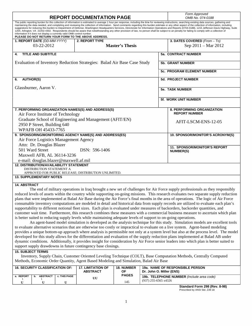
1
REPORT DOCUMENTATION PAGE Form Approved OMB No. 074-0188
The public reporting burden for this collection of information is estimated to average 1 hour per response, including the time for reviewing instructions, searching existing data sources, gathering and maintaining the data needed, and completing and reviewing the collection of information. Send comments regarding this burden estimate or any other aspect of the collection of information, including suggestions for reducing this burden to Department of Defense, Washington Headquarters Services, Directorate for Information Operations and Reports (0704-0188), 1215 Jefferson Davis Highway, Suite 1204, Arlington, VA 22202-4302. Respondents should be aware that notwithstanding any other provision of law, no person shall be subject to an penalty for failing to comply with a collection of information if it does not display a currently valid OMB control number. PLEASE DO NOT RETURN YOUR FORM TO THE ABOVE ADDRESS. 1. REPORT DATE (DD-MM-YYYY)
03-22-2012 2. REPORT TYPE
Master’s Thesis 3. DATES COVERED (From – To)
Sep 2011 – Mar 2012
4. TITLE AND SUBTITLE Evaluation of Inventory Reduction Strategies: Balad Air Base Case Study
5a. CONTRACT NUMBER
5b. GRANT NUMBER 5c. PROGRAM ELEMENT NUMBER
6. AUTHOR(S) Glassburner, Aaron V.
5d. PROJECT NUMBER 5e. TASK NUMBER
5f. WORK UNIT NUMBER
7. PERFORMING ORGANIZATION NAMES(S) AND ADDRESS(S) Air Force Institute of Technology Graduate School of Engineering and Management (AFIT/EN) 2950 P Street, Building 640 WPAFB OH 45433-7765
8. PERFORMING ORGANIZATION REPORT NUMBER AFIT-LSCM-ENS-12-05
9. SPONSORING/MONITORING AGENCY NAME(S) AND ADDRESS(ES) Air Force Logistics Management Agency Attn: Dr. Douglas Blazer 501 Ward Street DSN: 596-1406 Maxwell AFB, AL 36114-3236 e-mail: [email protected]
10. SPONSOR/MONITOR’S ACRONYM(S) 11. SPONSOR/MONITOR’S REPORT NUMBER(S)
12. DISTRIBUTION/AVAILABILITY STATEMENT DISTRIBUTION STATEMENT A APPROVED FOR PUBLIC RELEASE; DISTRIBUTION UNLIMITED. 13. SUPPLEMENTARY NOTES 14. ABSTRACT The end of military operations in Iraq brought a new set of challenges for Air Force supply professionals as they responsibly reduced levels of assets within the country while supporting on-going missions. This research evaluates two separate supply reduction plans that were implemented at Balad Air Base during the Air Force’s final months in the area of operations. The logic of Air Force consumable inventory computations are modeled in detail and historical data from supply records are utilized to evaluate each plan’s supportability to different notional fleet sizes. Each plan is evaluated under measures of backorders, backorder quantities, and customer wait time. Furthermore, this research combines these measures with a commercial business measure to ascertain which plan is better suited to reducing supply levels while maintaining adequate levels of support to on-going operations. An agent-based model simulation is developed as the analysis technique for this study. Simulation models are excellent tools to evaluate alternative scenarios that are otherwise too costly or impractical to evaluate on a live system. Agent-based modeling provides a unique bottom-up approach where analysis is permissible not only at a system level but also at the process level. The model developed for this study allows for the differentiation and evaluation of the supply reduction plans implemented at Balad AB under dynamic conditions. Additionally, it provides insight for consideration by Air Force senior leaders into which plan is better suited to support supply drawdowns in future contingency base closings. 15. SUBJECT TERMS Inventory, Supply Chain, Customer Oriented Leveling Technique (COLT), Base Computation Methods, Centrally Computed Methods, Economic Order Quantity, Agent Based Modeling and Simulation, Balad Air Base 16. SECURITY CLASSIFICATION OF: 17. LIMITATION OF
ABSTRACT
UU
18. NUMBER OF PAGES
145
19a. NAME OF RESPONSIBLE PERSON Dr. John O. Miller (ENS)
a. REPORT\
U
b. ABSTRACT\ U
c. THIS PAGE
U
19b. TELEPHONE NUMBER (Include area code) (937) 255-6565 x4326
Standard Form 298 (Rev. 8-98) Prescribed by ANSI Std. Z39-18