Embed Size (px)
Citation preview

EVALUATION OF INDEPENDENT MESH MODELING FOR
TEXTILE COMPOSITES
A Thesis
by
JEFFREY SCOTT MCQUIEN
Submitted to the Office of Graduate and Professional Studies ofTexas A&M University
in partial fulfillment of the requirements for the degree of
MASTER OF SCIENCE
Chair of Committee, John D. WhitcombCommittee Members, Mohammad Naraghi
Terry CreasyHead of Department, Rodney Bowersox
May 2017
Major Subject: Aerospace Engineering
Copyright 2017 Jeffrey Scott McQuien

ABSTRACT
The Independent Mesh Method (IMM) was used to analyze stress distributions
within a unit cell model for a symmetrically stacked plain weave textile composite.
Results from these analyses were compared to those of conventional finite element
analyses, which are well established. Preliminary comparisons showed extreme dis-
agreement between the two methodologies. Further investigation into the source of
these differences led to significant corrections to the IMM implementation. After
these updates, much better agreement between the two methodologies was observed;
however, noticeable differences were still present. The remaining differences were
characterized using a simple two-inclusion model upon which the impacts of the
penalty displacement method, which the IMM relies upon heavily, were more appar-
ent. It was shown that the implementation of the penalty displacement method for
maintaining approximate displacement continuity between two surfaces induces sig-
nificant error in stress distributions close to the interface. While these effects are less
noticeable in the plain weave model, they are still present and diminish the fidelity of
stress information in important tow-matrix interface regions, prohibiting the reliable
prediction of damage initiation and growth.
ii

DEDICATION
This thesis is dedicated to my father, without whom, it would have never been.
iii

ACKNOWLEDGEMENTS
I sincerely appreciate the guidance of my adviser Dr. John Whitcomb. It has been
a pleasure working under his leadership. I have ultimate respect for his capabilities as
a researcher and teacher, as well as for his unwavering standards. The opportunity
to work as his teaching assistant was a very enriching experience. In addition, I
would like to thank the members of my committee, Dr. Mohammad Naraghi and
Dr. Terry Creasy, for affording their time to see me through this education. I would
also like to thank Dr. Darren Hartl for supporting me through, and helping provide
the great experience of working on the morphing radiator research.
I greatly appreciate the help of the VTMS team at AFRL, Dr. David Mollen-
hauer, Dr. Endel Iarve, Eric Zhou, and Dr. Lauren Ferguson. I am thankful to have
had the opportunity to work closely with them over the summer, where the close
proximity allowed us to make significant progress.
My senior colleagues and fellow students Keith Ballard and Christopher Bertagne
did more than their fair share of answering my questions, and I give my thanks to
each. Keith has happily afforded himself as a resource, and I always know that if my
question ends up reaching him, it will get answered.
Lastly, I would like to thank my mother for her everlasting support.
iv

CONTRIBUTORS AND FUNDING SOURCES
This work was supported by a thesis committee consisting of Professors John
Whitcomb (advisor and chair of committee) and Mohammad Naraghi of the Depart-
ment of Aerospace Engineering, and Professor Terry Creasy of the Department of
Materials Science and Engineering.
All work conducted for this thesis was completed by the student under the over-
sight of the thesis committee and Dr. David Mollenhauer, Dr. Endel Iarve, and Eric
Zhou of the Air Force Research Laboratory.
v

TABLE OF CONTENTS
Page
ABSTRACT . . . . . . . . . . . . . . . . . . . . . . . . . . . . . . . . . . . . ii
DEDICATION . . . . . . . . . . . . . . . . . . . . . . . . . . . . . . . . . . . iii
ACKNOWLEDGEMENTS . . . . . . . . . . . . . . . . . . . . . . . . . . . . iv
CONTRIBUTORS AND FUNDING SOURCES . . . . . . . . . . . . . . . . . v
TABLE OF CONTENTS . . . . . . . . . . . . . . . . . . . . . . . . . . . . . vi
LIST OF FIGURES . . . . . . . . . . . . . . . . . . . . . . . . . . . . . . . . viii
LIST OF TABLES . . . . . . . . . . . . . . . . . . . . . . . . . . . . . . . . . xi
1. INTRODUCTION . . . . . . . . . . . . . . . . . . . . . . . . . . . . . . . 1
2. LITERATURE REVIEW . . . . . . . . . . . . . . . . . . . . . . . . . . . 10
2.1 Finite Element Analysis of Textile Composites . . . . . . . . . . . . . 102.1.1 Conventional finite element work . . . . . . . . . . . . . . . . 102.1.2 Non-conventional finite element work . . . . . . . . . . . . . . 13
2.2 Simulation of Textile Geometry . . . . . . . . . . . . . . . . . . . . . 162.2.1 Geometric based description . . . . . . . . . . . . . . . . . . . 162.2.2 Image enhanced geometric description . . . . . . . . . . . . . 182.2.3 Physics based simulation . . . . . . . . . . . . . . . . . . . . . 19
3. THEORY . . . . . . . . . . . . . . . . . . . . . . . . . . . . . . . . . . . . 23
3.1 Conventional Finite Element Formulation . . . . . . . . . . . . . . . . 233.1.1 Kinematic relationships . . . . . . . . . . . . . . . . . . . . . . 233.1.2 Constitutive relationships . . . . . . . . . . . . . . . . . . . . 253.1.3 Weak form derivation for elasticity . . . . . . . . . . . . . . . 283.1.4 Finite element model . . . . . . . . . . . . . . . . . . . . . . . 303.1.5 Element formulation . . . . . . . . . . . . . . . . . . . . . . . 33
3.2 Independent Mesh Method Adaptations . . . . . . . . . . . . . . . . . 383.2.1 Penalty displacement method . . . . . . . . . . . . . . . . . . 393.2.2 Approximation of resin domain . . . . . . . . . . . . . . . . . 40
vi

4. CONFIGURATIONS . . . . . . . . . . . . . . . . . . . . . . . . . . . . . . 43
4.1 Plain Weave . . . . . . . . . . . . . . . . . . . . . . . . . . . . . . . . 434.1.1 Geometry . . . . . . . . . . . . . . . . . . . . . . . . . . . . . 434.1.2 Mesh . . . . . . . . . . . . . . . . . . . . . . . . . . . . . . . . 444.1.3 Boundary conditions . . . . . . . . . . . . . . . . . . . . . . . 46
4.2 Two-Inclusion . . . . . . . . . . . . . . . . . . . . . . . . . . . . . . . 474.2.1 Geometry . . . . . . . . . . . . . . . . . . . . . . . . . . . . . 474.2.2 Mesh . . . . . . . . . . . . . . . . . . . . . . . . . . . . . . . . 494.2.3 Boundary conditions . . . . . . . . . . . . . . . . . . . . . . . 49
4.3 Material Properties . . . . . . . . . . . . . . . . . . . . . . . . . . . . 49
5. RESULTS . . . . . . . . . . . . . . . . . . . . . . . . . . . . . . . . . . . . 51
5.1 Plain Weave Model . . . . . . . . . . . . . . . . . . . . . . . . . . . . 515.1.1 Conventional plain weave analysis . . . . . . . . . . . . . . . . 525.1.2 Initial IMM plain weave analysis . . . . . . . . . . . . . . . . 565.1.3 Correction strategy . . . . . . . . . . . . . . . . . . . . . . . . 655.1.4 Final IMM plain weave analysis . . . . . . . . . . . . . . . . . 68
5.2 Two-Inclusion Model . . . . . . . . . . . . . . . . . . . . . . . . . . . 765.2.1 Conventional analysis . . . . . . . . . . . . . . . . . . . . . . . 765.2.2 IMM analysis . . . . . . . . . . . . . . . . . . . . . . . . . . . 785.2.3 Simplified case: single material property . . . . . . . . . . . . 835.2.4 Simplified case: rotated inclusion . . . . . . . . . . . . . . . . 85
6. CONCLUSIONS . . . . . . . . . . . . . . . . . . . . . . . . . . . . . . . . 92
REFERENCES . . . . . . . . . . . . . . . . . . . . . . . . . . . . . . . . . . . 94
vii

LIST OF FIGURES
FIGURE Page
1.1 Multi-scale analysis of textile composites . . . . . . . . . . . . . . . . 3
1.2 In plane photograph of a triaxial braided fabric, reprinted from [1] . . 4
1.3 Comparison of conventional and VTMS-IMM plain weave unit cellfinite element models . . . . . . . . . . . . . . . . . . . . . . . . . . . 6
3.1 8 node hexahedron master element . . . . . . . . . . . . . . . . . . . 34
3.2 Demonstration of X3D8 element construction showing a known geo-metric limitation . . . . . . . . . . . . . . . . . . . . . . . . . . . . . 42
4.1 Half-width tow cross section . . . . . . . . . . . . . . . . . . . . . . . 44
4.2 Full unit cell for symmetrically stacked plain weave . . . . . . . . . . 45
4.3 Eighth unit cell for symmetrically stacked plain weave . . . . . . . . . 45
4.4 Tow-matrix model configuration . . . . . . . . . . . . . . . . . . . . . 48
5.1 Meshes used in convergence study of conventional analysis . . . . . . 53
5.2 Mesh convergence of predicted effective modulus E11 for conventionalanalysis . . . . . . . . . . . . . . . . . . . . . . . . . . . . . . . . . . 54
5.3 Contour plots of σ11 for coarse conventional mesh . . . . . . . . . . . 57
5.4 Contour plots of σ13 for coarse conventional mesh . . . . . . . . . . . 58
5.5 Conventional model distribution of σ11 within transverse tow . . . . . 59
5.6 Conventional model distribution of σ13 within transverse tow . . . . . 59
5.7 Conventional model distribution of σ11 within axial tow . . . . . . . . 60
5.8 Conventional model distribution of σ13 within axial tow . . . . . . . . 60
5.9 Meshes used for initial IMM analysis . . . . . . . . . . . . . . . . . . 61
viii

5.10 IMM initial: comparison plots of σ11 for coarse mesh . . . . . . . . . 63
5.11 IMM initial: Comparison plots of σ13 for coarse mesh . . . . . . . . . 64
5.12 Initial IMM distribution of σ11 within transverse tow . . . . . . . . . 65
5.13 Initial IMM distribution of σ13 within transverse tow . . . . . . . . . 66
5.14 Initial IMM distribution of σ11 within axial tow . . . . . . . . . . . . 66
5.15 Initial IMM distribution of σ13 within axial tow . . . . . . . . . . . . 67
5.16 Meshes used in convergence study of IMM analysis . . . . . . . . . . 70
5.17 Mesh convergence of predicted effective modulus E11 for IMM anal-ysis, showing the converged result from the conventional analysis asthe horizontal . . . . . . . . . . . . . . . . . . . . . . . . . . . . . . . 71
5.18 IMM final: Comparison plots of σ11 for coarse mesh . . . . . . . . . . 72
5.19 IMM final: Comparison plots of σ13 for coarse mesh . . . . . . . . . . 73
5.20 Final IMM distribution of σ11 within transverse tow . . . . . . . . . . 74
5.21 Final IMM distribution of σ13 within transverse tow . . . . . . . . . . 74
5.22 Final IMM distribution of σ11 within axial tow . . . . . . . . . . . . . 75
5.23 Final IMM distribution of σ13 within axial tow . . . . . . . . . . . . . 75
5.24 Meshes used for conventional Two-Inclusion study . . . . . . . . . . . 77
5.25 Convergence of predicted elastic modulus for conventional Two-Inclusionstudy . . . . . . . . . . . . . . . . . . . . . . . . . . . . . . . . . . . . 78
5.26 Contour plots of σ11 for coarse conventional mesh . . . . . . . . . . . 79
5.27 Meshes used for IMM Two-Inclusion study . . . . . . . . . . . . . . . 81
5.28 Convergence of predicted modulus with respect to penalty parameterfor each mesh . . . . . . . . . . . . . . . . . . . . . . . . . . . . . . . 82
5.29 Convergence of predicted modulus with respect to mesh refinementfor each penalty parameter . . . . . . . . . . . . . . . . . . . . . . . . 82
5.30 Contour plots of σ11 for IMM using suggested penalty . . . . . . . . . 84
ix

5.31 Contour plots of σ11 for IMM using converged penalty . . . . . . . . . 84
5.32 Convergence of single property IMM Two-Inclusion model with re-spect to penalty parameter . . . . . . . . . . . . . . . . . . . . . . . . 85
5.33 Contour plots of σ11 for single property IMM two-inclusion models . . 86
5.34 IMM rotated two-inclusion mesh . . . . . . . . . . . . . . . . . . . . . 87
5.35 Convergence of predicted modulus with respect to penalty parameterfor IMM rotated two-inclusion model . . . . . . . . . . . . . . . . . . 88
5.36 Contour plots of σ11 for IMM rotated two-inclusion model using sug-gested penalty . . . . . . . . . . . . . . . . . . . . . . . . . . . . . . . 89
5.37 Contour plots of σ11 for IMM rotated two-inclusion model using con-verged penalty . . . . . . . . . . . . . . . . . . . . . . . . . . . . . . . 90
5.38 Volume distributions of σ11 within matrix . . . . . . . . . . . . . . . 91
5.39 Volume distributions of σ11 within inclusion . . . . . . . . . . . . . . 91
x

LIST OF TABLES
TABLE Page
3.1 Quadrature point locations and associated weights . . . . . . . . . . . 38
4.1 Material properties for tows and matrix . . . . . . . . . . . . . . . . . 50
5.1 Key metrics from conventional mesh convergence study . . . . . . . . 54
5.2 Facial displacements of fine mesh . . . . . . . . . . . . . . . . . . . . 55
5.3 Key metrics for initial IMM analysis . . . . . . . . . . . . . . . . . . 62
5.4 Key values from IMM mesh convergence study . . . . . . . . . . . . . 69
5.5 Tabulated results from conventional Two-Inclusion analyses . . . . . 77
5.6 Key metrics from IMM Two-Inclusion analyses . . . . . . . . . . . . . 82
5.7 Key metrics from IMM Rotated model . . . . . . . . . . . . . . . . . 88
xi
1. INTRODUCTION
Composite materials require additional analysis efforts than more conventional
engineering materials due to their inherently heterogeneous microstructures. Mul-
tiscale analysis methodologies have developed within the field of composites as one
approach to address this requirement. Since a composite material is defined by the
combination of one or more constituent materials, the resulting material usually has
at least two material scales. The smallest scale is defined by the length scale of the
smallest constituent, at which the material is heterogeneous, and the largest scale is
defined by the length scale at which the composite appears homogeneous. Multiscale
analysis is an approach in which results from analyses done at one scale are used to
model the behavior of the material at another scale. The end goal of the effort is
to understand the behavior of the composite enough such that it may be modeled
without representation of its constituents. It would not be practical to discretely
model every single reinforcement in a large concrete beam, or every carbon fiber
in an aircraft skin. At each particular scale there may be several analysis methods
available to choose from. These methods may be experimental, analytic, or numeri-
cal. Of course experimental methods, while the most realistic, are costly and require
the most time. Analytic methods can be very accurate but are difficult to apply to
complex structures. Numerical methods are the least expensive, and the least time
consuming given modern developments in computer technology. However, numerical
analyses are highly sensitive to the implementation of theory and to the parameters
involved in describing material behavior. Because of this, numerical methods are
developed and validated using experimental and analytic results. A validated nu-
merical analysis framework can be used to analyze a much higher volume of problems
1

than its counterparts. The finite element method is a powerful numerical analysis
framework capable of modeling at all material scales, and is the centerpiece of this
work.
Fiber reinforced composites are a popular engineering material on which multi-
scale analysis is often performed. Whether or not the fiber reinforced composite is
part of the unidirectional or textile class, the material scales can be defined by the
hierarchical breakdown of the composite material. Unidirectional composite laminae,
or mats, are made from the combination of fibers, that are all oriented in the same
direction, and resin. In classical composite nomenclature, the resin is referred to as
the matrix, and the fibers are referred to as the inclusions. These laminae are then
stacked into the resulting composite laminate. In order to understand the properties
of the laminate, the properties of the individual laminae must first be understood;
this establishes the basis for multiscale analysis. On the other hand, textile, or wo-
ven fabric, composites require an additional level of analysis. Figure 1.1 depicts the
hierarchical breakdown, or scales used in a multiscale approach, of a textile com-
posite component. A textile composite weaving tows, which are a combination of
fibers and resin, into a fabric mat. The resulting fabric mat can then be stacked
in a manner similar to the laminae of a unidirectional laminate. In this case the
lowest level of analysis is performed on the tow. Since the tow is a combination of
unidirectional fibers and resin, this analysis scale, Figure 1.1a, is identical to the
microscale analysis of the unidirectional fiber reinforced composites. The next scale,
Figure 1.1b, is defined by the length scale of the textile weave and is known as the
mesoscale. The mesoscale captures the effect of the weave morphology and contains
woven tows, whose properties are determined by the microscale analysis, and pockets
of pure resin. Mesoscale models are usually realized as unit cells, which capture all
of the geometry necessary to describe the fabric. Lastly the macroscale, Figure 1.1c,
2

(a) Microscale (b) Mesoscale (c) Macroscale
Figure 1.1: Multi-scale analysis of textile composites
is the scale at which the composite material is homogenized and is used to model
engineering parts. The present work is concerned with the geometric representation
of the textile at the mesoscale, and its analysis using the finite element method.
Mesoscale modeling is particularly challenging due to the complex geometries in-
herent in woven fabrics. In order to perform finite element analysis on a model at
this scale, the geometry must first be simulated and then discretized into a suitable
finite element mesh. Figure 1.2 shows an in-plane view of a triaxial braided com-
posite. Variability can be easily identified as tow widths change from tow-to-tow,
as well as along the length of an individual tow. Furthermore, each tow has unique
surface features which appear most frequently near the tow intersections. These
characteristics make it extremely difficult to realistically simulate textile geometry.
Consequentially, as geometry is more realistically simulated, its incorporation into a
finite element model becomes more difficult, particularly the formulation of the finite
element mesh.
Conventionally, the difficulty in accurately simulating mesoscale geometry is di-
minished by idealizing the tow architecture and weave pattern. This removes the
randomness present in the textile as discussed previously. By idealizing the tow ar-
chitecture it is possible to design a finite element mesh that fits each tow at every
3

Figure 1.2: In plane photograph of a triaxial braided fabric, reprinted from [1]
location. By idealizing the weave pattern it is possible to obtain mesh compati-
bility in a consistent manner throughout the finite element mesh. Idealizations of
these characteristics usually result in tow cross sections approximated as biconvex,
or elliptical, shapes, and sinusoidal tow paths. An early work based on this geo-
metric approach is outlined in [2]. The geometric representation, and its impacts, of
the analysis therein are thoroughly discussed in [3]. It is shown that the idealized
geometry can be completely characterized by the chosen tow path as well as the
cross sectional shape. All other model parameters are either directly or indirectly
determined by these two characteristics. Much of the work in analysis of textile com-
posites follows similarly. Obviously the idealization of textile geometric architecture
may have some impact on the results predicted by the analysis. A detailed investiga-
tion into the effect of including geometric randomness inherent in textile composites
has yet to be carried out. However, it has been shown in microscale analysis of fiber
composites that the consideration of geometric randomness has a significant impact
on results [4]. Mesoscale analyses lack a similar comparison due to the extreme diffi-
culty associated with first simulating a realistic geometry, and then performing finite
element analysis on it.
Recently a method was developed by Zhou et al. [5], which aims to simulate the
4

geometry of a textile composite at the mesoscale using a physics modeling technique
based on the multi chain digital element technique [6]. The resulting textile architec-
ture contains many features that are often observed in textiles, such as inconsistencies
in weave pattern, varying tow thicknesses across the width, and varying tow cross
sections along the tow path. The Virtual Textile Morphology Suite (VTMS), a tex-
tile analysis tool developed at the Air Force Research Laboratory (AFRL), is built
around an implementation of this digital element technique. As stated previously,
the difficulty in establishing a finite element mesh increases as the accuracy of geo-
metric simulation increases. VTMS is paired to AFRL’s B-Spline Analysis Method
(BSAM) finite element code, which makes use of a combination of unconventional
finite element techniques, referred to as the Independent Mesh Method (IMM), to
address this issue [7]1. First, each geometric entity is meshed independently and
compatibility between adjacent surfaces is imposed through a penalty displacement
method. A geometric entity is defined as a standalone body that is meshed inde-
pendently from all other entities. This is analogous to a part within an assembly in
many computer based design tools. In the context of textiles, each tow is an entity,
as well as the body of pure resin. Second, the mesh representing the body of pure
resin is generated using a technique similar to the extended finite element method
(XFEM). In the IMM approach, the resin is first represented as a background rectan-
gular structured grid mesh, with dimensions that encompass the volume of the tows.
The elements of the resin are then restructured based on the regions occupied by
tows. The shape functions of resin elements that are completely within the tows are
disregarded, and those belonging to elements that are intersected by the boundary
assume an adapted integration scheme. The portion of the element falling outside the
1The cited papers describe the original version of the IMM which makes use of a marching-cubeintegration mesh rather than tetrahedral
5

region occupied by the tow is supplemented with a set of integration points placed by
the insertion of tetrahedral integration elements. The IMM is more general than its
application to textiles, and as such may be described as choosing a set of geometric
entities which act as master surfaces, from which the other (background) entities
will be restructured as needed. In the case of the application to textiles, the tows
are defined as the master surfaces.
(a) Conventional plain weave unit cell using idealized geometry
(b) IMM plain weave unit cell mesh of VTMS simulated geometry
Figure 1.3: Comparison of conventional and VTMS-IMM plain weave unit cell finiteelement models
A comparison of side views of conventional and VTMS-IMM finite element models
6

is shown in Figure 1.3. Figure 1.3a shows a conventional finite element model using
idealized tow architectures. Each tow cross section is identical, and is constant along
the undulation of the tow. The specific geometry shown is produced using a sweeping
method rather than extruded, and has a relatively unrealistic waviness ratio [3].
There is perfect tow-to-tow and tow-to-resin mesh compatibility, as the entire domain
is discretized into a single finite element mesh. Figure 1.3b shows a comparable IMM
finite element model using tow architecture simulated by VTMS. Each tow cross
section is unique, and is not constant along the tow path. There is no tow-to-tow
or tow-to-resin nodal compatibility as each entity is meshed independently, and the
resin mesh is approximated using the IMM described above.
These additional finite element methods, while may be essential to analyzing
the realistic geometry produced by VTMS, may themselves introduce significant
errors on material behavior predictions. The objective of this work is to understand
what those impacts are, if any, and establish a method for minimizing them. The
systematic evaluation of these potential impacts will be carried out by implementing
the IMM on a model upon which a conventional finite element analysis may also be
used. The conventional analysis will serve as the benchmark. As discussed, there are
several factors that make the IMM approach different from that of a conventional
finite element approach. The IMM approach:
• Is able to consider complex geometries without burdening the meshing process.
• Uses an unconventional element formulation to model the volumes of pure resin
within the unit cell.
• Uses a penalty method to impose displacement continuity between separate,
independent mesh entities, which may or may not have compatible surface
meshes.
7

Regarding the above list, each item requires the use of the items below it given
the implementation of the IMM. Since the evaluation performed in this work requires
the use of a conventional analysis as benchmark, the first item can not be considered.
The production of a compatible mesh for the VTMS simulated geometry, suitable
for use with conventional finite elements, may in fact be possible, but the meshing
process would be cumbersome. In addition, the IMM would not be necessary given
a compatible mesh. As such, the current evaluation will focus on the implications
of the IMM characteristics outlined in the second and third bullets. It is possible
to invoke each of these IMM characteristics upon a textile model that is otherwise
suitable for use with conventional finite element methods. The evaluations herein
make use of identical geometries between conventional and IMM models. The meshes
for master entities in the IMM model are identical to the corresponding meshes in
the conventional model, save for the separation into standalone entity meshes. The
resin mesh in the IMM models, while having the same geometry as the corresponding
conventional models, will be constructed in the IMM manner described previously.
In this way, both of the characteristics of the second and third bullets are present in
the IMM models.
This thesis begins with a review of the literature relevant to the modeling and
analysis of textile composites. First, the body of work in three dimensional finite
element analysis of textile composites is discussed. Second, the existing methods for
simulation of textile geometry are presented, as well as some meshing related efforts.
A theory section then describes the finite element formulations relevant to both the
conventional and IMM approaches used herein. Next, the analysis configurations
used in evaluation of the IMM are detailed. The first configuration is a plain weave
textile unit cell as the chosen textile composite model for evaluation. The second
configuration discussed is a simplified two-inclusion model upon which all character-
8

istics of the IMM can be implemented in a manner where their impacts are more
readily observable than with the textile. Results of the two analysis configurations
are then presented. An investigation into the behavior of the penalty method under
various refinements and weights is given in the context of the two-inclusion configu-
ration. Solution convergences, as well as comparisons of the predicted stress fields,
are presented for both configurations using suitable refinements and penalty weight.
Lastly, a summary of the results, the conclusions drawn, and the direction of future
work is provided.
In an effort to more accurately model and analyze the behavior of textile com-
posites, new techniques are being developed. This work hopes to establish an un-
derstanding of one such new technique, to provide a foundation for it to be used in
analysis of complex textile architectures upon which other analysis methods can not
be readily used.
9

2. LITERATURE REVIEW
Mesoscale modeling is central to the analysis of textile composites. As such, there
is significant literature regarding analysis methods. This chapter presents a cursory
review of previous work and state of the art in mesoscale finite element analysis of
textile composite unit cells, as well as the methods by which the geometry in those
models was produced. First, the significant contributions to the finite element anal-
ysis are discussed. Second, the body of work pertaining to the creation or simulation
of textile geometry is presented.
2.1 Finite Element Analysis of Textile Composites
The works presented in this section focus on analyses intended to investigate
the distribution of local stresses within the unit cell for purposes of understanding
how the geometry affects stress distributions and ultimately damage. Many ana-
lytic methods, and many finite element analyses, have been developed for mesoscale
models with the sole purpose of stiffness prediction; these types of methods are not
discussed. The works presented first cover conventional finite element techniques
which use conventional element formulations and compatible meshes, and then non-
conventional methods.
2.1.1 Conventional finite element work
Perhaps the first finite element analysis of a textile composite, geared toward
stress analysis, was accomplished by Whitcomb in [2]. In this work, three dimen-
sional finite element analysis is performed on a plain woven composite unit cell. The
unit cell was modeled using idealized geometry and meshed with linear elastic el-
ements. Several different plain woven geometries were analyzed to determine the
10

effect of tow waviness on the effective material properties and internal stress and
strain distributions. It was shown that tow waviness and predicted effective moduli
were directly related. Although this work was limited to linear elastic analysis, such
that damage propagation could not be investigated, the work defines the basis for
three dimensional stress analysis of a textile unit cell. In a later work, Whitcomb
and Tang extend the study of the effect of waviness on effective stiffnesses to satin
and twill woven composites [8].
Blackketter et al. developed a three dimensional finite element model for the
plain weave composite for damage analysis in [9]. Effective constitutive properties
for the tows were evaluated using a lower scale micro-mechanical model of fibers
and matrix. The unit cell was modeled using idealized geometry, and damage was
modeled using a non-linear stiffness reduction scheme developed by the authors. In
the analyses, both tension and shear loadings were investigated, and results compared
well with experimental data. It was shown that non-linear behavior under shear was
principally due to damage propagation rather than plasticity in the matrix.
Chapman and Whitcomb investigated the effects of geometric approximations on
plain weaves in [3]. In this work the textile was modeled using idealized geometry
with lenticular shaped tow cross sections, full contact between tows, and sinusoidal
tow paths. The focus of the investigation was the effects of modeling the tow ge-
ometry by sweeping the tow cross section along the tow path, or simply translating
it. When a constant cross section is swept, it remains orthogonal to the tow path,
and when it is translated the constant cross section remains vertical, i.e. it does not
rotate. The difference in geometry is subtle at low tow waviness (the amplitude of
the sinusoidal tow path) and is amplified at high waviness. A translated constant
cross section distorts the volume of the tow at high waviness. The results of the
stress analysis for the two geometric representations follow the same trend.
11

Whitcomb and Srirengan carried the studies of geometric approximations and
mesh characteristics into failure analysis of plain weave composites in [10]. Several
model characteristics were studied including quadrature order, mesh refinement, the
chosen damage model, and tow waviness. Notably, the predicted strength was ob-
served to decrease significantly as tow waviness increased. Tow waviness was also
shown to affect the stress at which damage initiates, and the stress component re-
sponsible for furthering damage was shown to change as damage progressed.
Thom supplemented the investigation into the effects of certain geometric and
mesh related approximations on the stress analysis of plain weave composites in
[11]. While Chapman and Whitcomb explored the effects of tow waviness and the
methods by which the tow volume is geometrically constructed from the tow cross
section, Thom evaluated the influence of mesh refinement, the size of the unit cell
volume occupied by pure matrix, the shape function of the tow path, and linear
versus non-linear analysis. Thom concludes that the best way to model gaps in the
fabric, within a single ply, is to model the tow cross section with a blunt edge. This
allows pockets of pure resin to be modeled between the tows without the need for
a step in tow curvature, or for out of plane separation between the tows, as done
by Dasgupta et al. in [12], which eliminates the tow-to-tow contact. The proposed
elliptical tow path, as opposed to sinusoidal, is observed to have strong influence on
the stiffness and peak stress distributions. Linear analysis is determined sufficient
for laminates.
Carvelli and Poggi developed a two step homogenization procedure to predict
both the stiffness and strength of woven fabric laminates in [13]. A fiber matrix
representative volume element (RVE) is first analyzed to predict effective mechanical
properties for tows, given a specified fiber volume fraction. The fibers in the fiber
matrix RVE are modeled assuming periodic hexagonal packing. The effective tow
12

properties were then used to model a 3 harness satin unit cell in a three dimensional
finite element damage model. The goal of the work was to develop the framework
in a manner suitable for implementation in commercially available finite element
software.
Whitcomb et al. developed methods for obtaining boundary conditions for peri-
odic analysis of textile composites and for reducing domain size by exploiting mate-
rial symmetries in [8]. Periodic boundary conditions are developed for a 1/32 region
of a symmetrically stacked plain weave unit cell and for a 1/2 region of a simply
stacked 8-harness satin weave unit cell. These techniques are generalized by Tang
and Whitcomb in [14].
Goyal and Whitcomb analyzed the effects of braid angle, waviness, material prop-
erties, and cross sectional shapes in 2 x 2 biaxial braided composites in [15, 16]. In
these analyses it was shown that braided fabrics see higher stress concentrations
than other comparable fabrics. Stress concentrations were observed to be highly
influenced by braid angle, and increased nearly linearly with waviness.
2.1.2 Non-conventional finite element work
One of the limiting factors of all of the above mentioned work is the approximation
of geometry by idealization. As mentioned previously, even after this approximation,
creating a suitable finite element mesh still presents a difficult task. And as less
geometric idealizations are made the task of meshing becomes harder. This theme
has been addressed in the literature in several ways. One is to develop new algorithms
for producing conventional finite element meshes, sometimes referred to as conformal,
for models with complex geometry. Another is to adapt the finite element formulation
to use non-conventional element formulations, or a non-conformal mesh. Either way,
the issue being addressed is the same: generating a suitably detailed finite element
13

mesh for textile composites is challenging.
Woo and Whitcomb implemented a Global/Local finite element method for textile
composites using macro finite elements [17, 18]. This method was developed to
address issues in computing time and resources by removing the need for a highly
detailed finite element mesh for the entire domain. By the use of the so called
macro finite elements, a relatively coarse (global) mesh could be constructed for a
large domain using homogenized material properties, with subdomain (local) meshes
constructed for regions of interest to enhance the information at the global level. The
subdomain meshes would discretely model the heterogeneous constituents within the
domain. Results from the global analysis, namely displacements at nodes along the
global/local boundary, were used to define the boundary conditions on the subdomain
analyses. The results of the subdomain analyses would then be used to influence
the forces at the global level. Although this method is proven effective at reducing
computation time and resources, the stress-strain distributions were shown to contain
significant error near the global/local boundary.
Cox et al. developed the Binary Model for textile composites to circumvent the
need for generating complex meshes [19, 20]. In this model, one dimensional elements
are used to represent tow axial stiffness, and are arranged to follow a tow’s path in
a piecewise linear fashion. The one dimensional line elements are then fixed within
three dimensional elements through the use of multipoint constraints. The three
dimensional elements represent what the authors term the effective medium that is
dominated by the matrix constitutive properties. Because of this approximation, the
model is capable of predicting effective stiffnesses but lacks sufficient information
for predicting failure. To this end, the author’s supplemented the model with a
specialized strain averaging technique and a method for predicting strength [21, 22].
Belytschko et al. developed what is known as the Structured Extended Finite
14

Element Method (XFEM) as a means for modeling geometrically complex solids
without the need for constructing a mesh that conforms to the geometry. Although
not developed explicitly for textile composites, XFEM has found applications in the
field. Within the XFEM framework, characteristics such as material interfaces or
cracks are defined as implicit surfaces within elements, and represented using radial
basis functions. Because of this, the entire domain can be meshed using a structured
mesh, while the geometric complexities are transferred to the model by the implicit
surfaces defined by mathematical equations. The XFEM formulation is sufficiently
complex on its own and will not be discussed in detail herein.
Jiang et al. developed the Domain Superposition Technique (DST) for model-
ing textile composites [23]. In DST, the volumes of tows and matrix are meshed
separately, while the matrix occupies the entire volume of the textile unit cell, and
then the two meshes are superimposed to produce a combined model. The matrix
mesh is structured and has no need to conform elements to the tow-matrix mate-
rial interfaces. The elements of the matrix mesh are assigned material properties
corresponding to the actual matrix, and the elements of the tow mesh are assigned
material properties based on the difference between the matrix and tow properties.
Continuity between the matrix and tow meshes is handled using a constraint cou-
pling technique which requires the nodal displacements of the tow meshes to be equal
to that of the global matrix mesh. This method does not make use of an iterative
procedure, as opposed to the mesh superposition techniques developed by Fish et al.
[24], which have been adapted for use in textile composites.
Kumar et al. developed a method for performing finite element analysis using a
nonconforming mesh [25, 26]. In this method, the entire analysis domain, regardless
of internal and external geometry, is meshed using a structured grid. Any external or
internal geometric features are represented using implicit surfaces defined by math-
15

ematical equations, which take the form of approximate step functions and are used
to evaluate the volume integrals. This method has many characteristics of XFEM,
but uses a specialized method for imposing boundary conditions which the authors
refer to as the Implicit Boundary Method (IBM).
Tabatabaei et al. proposed an alternative method for meshing textile compos-
ites which they refer to as the Embedded Element (EE) technique [27, 28]. In the
EE technique, the matrix and tows are meshed separately, with the matrix volume
covering the entire domain, and then the tow mesh is embedded within the matrix
mesh. The degrees of freedom of the embedded mesh (the tow mesh) become slave
to interpolated values of corresponding degrees of freedom of the host mesh (the
matrix mesh). A description of the constitutive model for the overlapping region is
not supplied. The EE is geared toward implementation in commercial finite element
software.
2.2 Simulation of Textile Geometry
Much of the work done in textile geometry simulation is accomplished in tandem
with stress analysis, but this review will focus on the production of geometric descrip-
tions for purposes of finite element meshing. The methods of geometry simulation
fall into three camps: either the geometric architecture is solely based on geomet-
ric data, the architecture is enhanced using image based analysis, or it is produced
through physics based simulation. Work belonging to each camp will be discussed.
2.2.1 Geometric based description
Peirce proposed the first significant model of fabric geometry where tow (yarn or
thread) cross sections were circular [29]. In this model, tow paths were represented in
a series of straight lines and circular arcs. Thus the straight lines represent the undu-
lating portion of the tow path, and the circular arc represents the cross over region,
16

where the tow path arcs around the cross section of the adjacent tow maintaining
full tow-to-tow contact. The linear region of the tow path is the most significant
limitation of this model, because in reality the bending stiffness of the fibers would
not lead to such a linear path.
Kemp further developed the Peirce geometry with the proposition of the racetrack
tow cross section in [30]. This cross section takes the form of two circular arcs
attached to the opposing ends of a rectangular cross section. A fabric which maintains
tow-to-tow contact in the crossover regions would therefore have a linear section of
the tow path as it crosses over an adjacent tow. The tow path therein is still a
combination of linear sections and circular arcs. While the racetrack cross section is
certainly more representative of the true flattened cross sectional shape of tows, it is
still not very accurate.
Hearle and Shanahon proposed a new lenticular tow cross sectional shape in
[31, 32]. The lenticular cross section is created by two opposing circular arcs with an
offset between their center points. When the center points are coincident, the cross
section is circular. A fabric maintaining full tow-to-tow contact in cross over regions
will have its tow path predominantly defined by the cross section itself. When there
are no linear regions in the tow path, the cross section completely defines the tow
path. This cross sectional representation is widely accepted as a sufficient description
of the flattened fabric geometry.
Hivet and Boisse developed an automated CAD geometry based simulation of
fabrics [33]. In this framework, the cross sections of tows are formed using four
customizable line segments. Each line segment can take the form of a straight line
or parabola. Tow paths are driven by the cross sections of adjacent tows to maintain
tow-to-tow contact. When more than two tows are in contact, straight line segments
are used to simplify the tow cross section. Tow paths in contact free zones are straight
17

in light of minimal bending stiffness. In this way, tow cross sections vary along the
length of the tow. The method was implemented for two dimensional fabrics e.g.
plain, satin, and twill woven fabrics.
The works of Robitaille et al. [34, 35, 36, 37] formed the basis for the textile
geometry simulation and finite element meshing software TexGen. TexGen is an
integrated textile modeling and analysis software package built upon a generalized
textile geometry construction methodology. TexGen is capable of modeling two di-
mensional and three dimensional textile architectures. In TexGen, all geometries for
all types of textile reinforcements are simulated using a series of vectors representing
the tow centerlines. Tow paths are constructed from the vectors by adjoining vector
endpoints using circular arcs with first order continuity for smoothing. Tow cross
sections, either elliptical or lenticular, are then swept along the tow paths to create
solid bodies. In later versions, this smoothing process using vectors and circular arcs
was replaced with a series of control points defining the tow path and the use of
Bezier and Cubic interpolations for smoothing. TexGen uses input data obtained
from observations of real textiles to influence the tow paths, which are otherwise
arbitrarily placed. Tow cross sections are tailorable to remove interpenetrations and
do not necessarily remain constant along the tow length.
2.2.2 Image enhanced geometric description
Kim and Swan suggested a voxel based meshing method in [38]. This tech-
nique uses three dimensional pixels, or voxels, obtained from image processing com-
bined with an adaptive, automated meshing technique [39] to produce locally refined
meshes which describe the complex three dimensional textile architecture. Using
only the voxel based methodology, a structured hexahedral mesh is created that cov-
ers the entire textile unit cell domain. Each voxel (easily convertible to a hexahedral
18

element) is assigned a material or mixture of material depending on where it lies
in mathematically defined sub-domains which describe the shape of the tows and
matrix. The voxels which are assigned multiple materials are ultimately handled by
being prescribed a material property set that is based on a rule of mixtures. The
adaptive, automated refinement technique was therefore developed to refine these
mixed material voxels into tetrahedral elements with a single material property.
While these models produce accurate estimates of elastic stiffnesses, the character-
ization of material interface regions are limited due to the shape of voxels and the
subsequent artificial tetrahedral refinement. This limitation impedes accurate dam-
age modeling.
Potter et al. describe a further developed voxel based meshing method which bet-
ter captures the definition of material interfaces in [40]. The material interfaces are
improved by using a voxel smoothing technique borrowed from the biomedical field
[41]. The developed framework is capable of producing smooth surface hexahedral
meshes, directly from the initial voxel description which contains ”jagged” material
interfaces by nature. Support for the application of periodic boundary conditions is
available, and the meshing algorithm contains generality for handling architectural
deformity within the textile.
2.2.3 Physics based simulation
Sherburn et al. proposed an energy minimization technique for predicting textile
geometry in [42]. In the proposed method, a representation of geometry is initially
obtained (namely, from the authors’ modeling software TexGen) and then augmented
using a finite element based numerical procedure. The initial geometric representa-
tion is fitted with plate elements along tow midsurfaces, capturing the tow bending
and tensile properties. Contacts between materials are modeling using a penalty
19

function weighted proportionally to interpenetration distance. Displacements of the
tows are captured when solving for the minimum energy configuration and then used
to modify the initial geometric representation. The resulting geometry is shown to
compare more accurately to textile micrographs than the original.
Lomov et al. have developed a textile modeling and analysis software called
WiseTex [43, 44, 45, 46, 47, 48]. Like TexGen, WiseTex is an integrated geometric
modeling and analysis software package that supports many types of two dimensional
and three dimensional textile architectures. WiseTex uses a combination of several
analytic models, educated by physical properties of the fabric, to calculate the tex-
tile geometry in its relaxed state. In this way, the software starts with a general
description of a textile containing the weave pattern and initial tow cross sectional
shapes, and then employs an analytic energy minimization procedure to calculate
the relaxed configuration. This process requires input data describing the physical
properties of the fabric determined experimentally. For example, Desplentere et al.
studied variability in micro-ct scans of 3d warp knitted textile composites to build
geometric data sets for input into WiseTex in [49].
Perhaps the most general method for simulating the geometry of textile compos-
ites is the mechanical based simulation of the multi-chain digital element technique
[6, 5]. This method attempts to reproduce the entire weaving and relaxation process
by directly modeling the mechanical behavior of fibers, represented by multi-chain
digital elements, and bundles of fibers woven together in a specified pattern and
placed under tension. Due to computational expenses, tows are modeled as a bundle
of an arbitrary number of fibers, or multi-chain digital elements, usually between 15
and 80. The relaxation process is an iterative procedure that applies tension to the
ends of each fiber, calculates a displacement, and then the resulting interaction with
the other fibers. Multi-chain digital elements are essentially a series of spherical ele-
20

ments along a string; when these elements come into contact with eachother, contact
forces are generated to cause a reaction. After the fabric is sufficiently relaxed, geo-
metric calculations can be performed to form solid boundaries encasing each bundle
of fibers to form tow volumes. This modeling process is general and can be applied
to a number of different weave patterns, tow diameters, and spacings. Resulting
geometries closely resemble observed fabrics. Limitations of this methodology are
related to finite element meshing of the produced geometry, as discussed throughout
this thesis.
Drach et al. developed a finite element meshing framework in [50] for the purposes
of creating high quality, conformal finite element meshes for geometry produced by
an implementation of the multi-chain digital element technique [6] in DEA Fabric
Mechanics Analyzer (DFMA). It is important to note that the present thesis is
focused on the IMM, which was developed for obtaining, and utilizing, non-conformal
finite element meshes for geometry produced by a separate implementation of the
multi-chain digital element technique in VTMS.
Grail et al. attacked the problem of generating conforming finite element meshes
for complex geometries in [51]. Geometric models of textiles that result from model-
ing compaction and relaxation often contain complexities, such as interpenetrations,
that make traditional finite element meshing very difficult. These complexities can
be dealt with by adjusting the cross sections of tows such that they are not in contact,
but this introduces artificial matrix layers. The authors describe algorithms for en-
suring mesh compatibility between tows that have come into contact with eachother.
In practice, when geometric descriptions of two tows in contact are meshed, the re-
sulting mesh contains interpenetrations. This is due to the reduction in geometric
fidelity when fitting finite elements to the boundaries. The algorithms described
therein are capable of removing these interpenetrations, while maintaining smooth
21

tow surfaces, and producing conformal tow surface meshes.
To date, there has been substantial work in the modeling and analysis of textile
composites. While conventional approaches which make use of idealized geometries
are well established, novel approaches for simulating more realistic geometric descrip-
tions are just emerging. These newer approaches come along with modifications to
the finite element formulations which are used to analyze them. Little to no work
has been done to evaluate the significance of these more realistic textile geometries.
22

3. THEORY
This chapter details the theory behind the tools used to perform the analyses in
this work. The conventional formulation of elastic finite elements in three dimensions
is presented first. Then the IMM adaptations are discussed.
3.1 Conventional Finite Element Formulation
This section develops what is referred to herein as conventional finite element
analysis, which is an implementation of the three-dimensional elastic finite element
method. Finite element analysis is based on the discretization of the analysis domain
into elements, or a mesh. These elements are assigned various constitutive properties
corresponding to the material which occupies its volume. Element stiffnesses are
developed from these constitutive properties to satisfy the governing equilibrium
equations. Boundary conditions are formed through the specification of either force
or displacement over the entire boundary of the mesh. These boundary conditions,
together with the element stiffnesses, are used to form a system of linear equations
for equilibrium. The solution of this system is the collection of nodal forces and
displacements for equilibrium. Through the use of kinematic relationships, full field
strains can be calculated from these displacements. Stresses are then obtained using
the constitutive relationships. The following sections discuss these operations in
detail.
3.1.1 Kinematic relationships
3.1.1.1 Spatial description
There are two reference frames for describing the deformation of a material. The
Lagrangian, known as the material description, is formed in terms of the undeformed
23

configuration where a material point is denoted by reference coordinates Xi. The
second reference frame, the Eulerian frame, known as the spatial description, is
formed in terms of the deformed configuration where material points are defined by
the spatial coordinates xi. A mapping function exists relating a point in the deformed
material xi to its reference point Xi and is shown in Equation 3.1.
xi = χ(Xi, t) (3.1)
In the case where t = to, the above equation results in xi = Xi = χ(Xi, to).
3.1.1.2 Displacement
Given Equation 3.1, which provides the Eulerian description in terms of the Lan-
grangian, it is straightforward to form an expression for displacement. The definition
of displacement in Equation 3.2 is the change in position of a material point from
its reference configuration to its deformed configuration, and is written entirely in
terms of the Lagrangian description with the assistance of Equation 3.1.
ui = xi −Xi (3.2)
3.1.1.3 Infinitesimal strain
The deformation gradient, F , is defined in Equation 3.3 where the Kronecker
delta δij is used for simplicity.
Fij =∂xi∂Xj
=∂χ(Xi, t)
∂Xj
=∂ui∂Xj
+ δij (3.3)
From the deformation gradient the right stretch tensor, C, also known as the
24

right Cauchy-Green deformation tensor, is computed as in Equation 3.4.
Cij = FkiFkj (3.4)
The Green-Lagrange strain tensor is defined as, and obtained using, Equation 3.5.
Eij =1
2(Cij − δij)
=1
2
(∂ui∂Xj
+∂uj∂Xi
+∂uk∂Xi
∂uk∂Xj
) (3.5)
Lastly the linearized infinitesimal strain tensor, ε, is derived assuming that the
second order term in Equation 3.5 is negligible given the linearizing assumption, and
that ∂ui∂Xj≈ ∂ui
∂xjgiven that strains are small. This results in Equation 3.6.
εij =1
2
(∂ui∂Xj
+∂uj∂Xi
)≈ 1
2
(∂ui∂xj
+∂uj∂xi
) (3.6)
Given this description, the difference between the Eulerian and Langrange de-
scriptions becomes negligible, and all spatial coordinates can be given in the form
xi. The infinitesimal strain tensor is also shown to be symmetric by definition since
it contains the addition of a matrix and its transpose.
3.1.2 Constitutive relationships
The constitutive rule provides a relationship between stress and strain, and ul-
timately between loads and deformation. The linear elastic constitutive model is
based on Hooke’s law, which proposes a linear relationship between stress and strain
described by a fourth order tensor Cijkl, known as the stiffness tensor. The stress
25

strain relationship, in the absence of thermal strains, is shown in Equation 3.7.
σij = Cijklεkl (3.7)
The fourth order tensor, Cijkl, is Cartesian based such that it contains 81 unique
entries, or independent constants. However, due to the noted symmetry in the strain
tensor, as well as similar symmetry in the stress tensor required for equilibrium of
angular momentum, the number of unique entries can be reduced by the relations
Cijkl = Cjikl = Cijlk. This is known as the minor symmetry and results in the
following matrix-expanded relationship.
σ1
σ2
σ3
σ4
σ5
σ6
=
C11 C12 C13 C14 C15 C16
C21 C22 C23 C24 C25 C26
C31 C32 C33 C34 C35 C36
C41 C42 C43 C44 C45 C46
C51 C52 C53 C54 C55 C56
C61 C62 C63 C64 C65 C66
·
ε1
ε2
ε3
ε4
ε5
ε6
(3.8)
Equation 3.8 uses contracted notation such that the subscripts (1, 2, 3, 4, 5, 6)
correspond to the expanded subscripts (11, 22, 33, 23, 31, 12). Also, the shearing
strains equal twice their tensorial values. A further reduction in independent con-
stants can be made through the major symmetry of the stiffness matrix observed
through the strain energy function, Equation 3.9, which should be insensitive to the
order of ij and kl indices.
U = Cijklεijεkl = Cklijεijεkl (3.9)
26

With the major symmetry stating that Cijkl = Cklij, the constitutive relationship
shown in Equation 3.8 simplifies to Equation 3.10, where there remain 21 nonzero
independent constants.
σ1
σ2
σ3
σ4
σ5
σ6
=
C11 C12 C13 C14 C15 C16
C12 C22 C23 C24 C25 C26
C13 C23 C33 C34 C35 C36
C14 C24 C34 C44 C45 C46
C15 C25 C35 C45 C55 C56
C16 C26 C36 C46 C56 C66
·
ε1
ε2
ε3
ε4
ε5
ε6
(3.10)
This is the general stiffness tensor for an anisotropic material, and can be sim-
plified further by appealing to a particular material symmetry. This is done by
transforming the stiffness tensor according to the material symmetries, and impos-
ing invariance. The analysis tools used in this thesis make use of material files ca-
pable of describing a material with orthotropic symmetry. An orthotropic material
has three orthogonal plains of symmetry and after simplification its stiffness tensor
contains 12 nonzero entries with only 9 independent constants. These constants are
most conveniently described through the compliance tensor, S, which is the inverse
of the stiffness tensor. The compliance tensor for an orthotropic material is shown
in Equation 3.11, relating strain to stress using engineering properties. Recall the
major symmetry of the stiffness tensor such that the relations ν12E1
= ν21E2
, ν13E1
= ν31E3
,
and ν23E2
= ν32E3
exist, meaning that only 9 of the 12 total engineering constants are
27

independent.
ε11
ε22
ε33
2ε23
2ε31
2ε12
=
1E1
−ν21E2−ν31
E30 0 0
−ν12E1
1E2
−ν32E3
0 0 0
−ν13E1−ν23
E2
1E3
0 0 0
0 0 0 1G23
0 0
0 0 0 0 1G31
0
0 0 0 0 0 1G12
·
σ11
σ22
σ33
σ23
σ31
σ12
(3.11)
The meanings of the engineering constants used in Equation 3.11 are as follows:
the Ei are the Young’s moduli in the i directions, the Gij are the shear moduli in
the ij planes, and the νij are the Poisson ratios for transverse strain in the j direc-
tion when stressed in the i direction. In this work, materials will either be assigned
transversely isotropic material properties, or isotropic material properties. Trans-
verse isotropy is a material symmetry that, in addition to orthotropic symmetry,
contains a rotational symmetry about one axis, usually the first. The transverse
isotropic stiffness matrix contains 12 nonzero entries that can be characterized using
5 independent constants. Isotropy is a material symmetry that, in addition to trans-
verse isotropy, contains rotational symmetry about the remaining two axes. The
isotropic stiffness matrix contains 12 nonzero entries that can be characterized using
only 2 independent constants.
3.1.3 Weak form derivation for elasticity
The finite element formulation for elasticity begins with the equation for equilib-
rium of a deformable body given by Equation 3.12.
∂σij∂xj
+ fi = 0 (3.12)
28

Following the principle of virtual work, Equation 3.12 is then multiplied by virtual
displacements, δui, and then integrated over the domain V to produce the weighted
residual. ∫V
δui
(∂σij∂xj
+ fi
)dV =
∫V
(δui
∂σij∂xj
+ δuifi
)dV = 0 (3.13)
Integrating the first term in Equation 3.13 by parts results in Equation 3.14.
∫V
(∂(δuiσij)
∂xj− σij
∂δui∂xj
+ δuifi
)dV = 0 (3.14)
The divergence theorem can then be applied to the first term in Equation 3.14
to result in Equation 3.15 where S represents the boundary of the volume V .
∫S
(δuiσijnj) dA+
∫V
(δuifi − σij
∂δui∂xj
)= 0 (3.15)
Now, Cauchy’s stress formula which relate stress to tractions, T , at the boundary
is given by Equation 3.16. In addition, the implication of symmetry in the stress
tensor, as well as Equation 3.6, allow for the following product to be rewritten as in
Equation 3.17.
Ti = σijnj (3.16)
∂δui∂xj
σij = δεijσij (3.17)
Equation 3.16 together with Equation 3.17 can be substituted into Equation 3.15
to yield the following final weak form.
∫S
(δuiTi) dS +
∫V
(δuifi − σijδεij) dV = 0 (3.18)
29

3.1.4 Finite element model
The displacements within a finite element ui, which are governed by Equa-
tion 3.18, are approximated by a sum of interpolation functions multiplied by nodal
displacements. Within an element containing n nodes, each node has an associated
interpolation function ψm, where the superscript m denotes the node. The interpo-
lation functions are formed such that ψm has the value 1 at the mth node, and 0 at
all other nodes in the element. This leads to the approximations for displacement
and virtual displacement given by Equations 3.19 and 3.20.
ui =n∑
m=1
umi ψm (3.19)
δui =n∑
m=1
δumi ψm (3.20)
In the above expressions the umi denotes the nodal displacements at node m. It is
convenient to form the vector q containing all components of all nodal displacements,
or degrees of freedom, in a given element.
q =
[u11, u12, u13, . . . , um1 , um2 , um3 , . . . , un1 , un2 , un3
](3.21)
With this vector, q, the virtual displacement, Equation 3.20, and the virtual
strain, Equation 3.17, can be written as the following.
δui =∂ui∂qα
δqα (3.22)
δεij =∂εij∂qα
δqα (3.23)
Applying the weak form to the element and substituting in the above expressions
30

produces the following.
∫Se
(∂ui∂qα
δqαTi
)dSe +
∫Ve
(∂ui∂qα
δqαfi − σij∂εij∂qα
δqα
)dVe = 0 (3.24)
In Equation 3.24, the subscript, e, on the integral limits, signifies that the inte-
gration is done over a single element. The δqα can be factored out from the integrals,
and it can be observed that since Equation 3.24 must hold true for any arbitrary
value of δqα, the following must be true.
∫Se
(∂ui∂qα
Ti
)dSe +
∫Ve
(∂ui∂qα
fi − σij∂εij∂qα
)dVe = 0 (3.25)
After rearranging,
∫Ve
(σij∂εij∂qα
)dVe =
∫Se
(∂ui∂qα
Ti
)dSe +
∫Ve
(∂ui∂qα
fi
)dVe (3.26)
This expression is now rewritten in familiar finite element terms. The left hand
side of Equation 3.26 can be simplified by making the use of contracted notation
such that,
εi = [ε11, ε22, ε33, 2ε23, 2ε13, 2ε12]T (3.27)
σi = [σ11, σ22, σ33, σ23, σ13, σ12]T (3.28)
as well as the introduction of the the strain-displacement matrix, B, which contains
31

the partials of the interpolation functions used in calculating strains.
B =∂εk∂qα
=
∂ψ1
∂x10 0 . . . ∂ψn
∂x10 0
0 ∂ψ1
∂x20 . . . 0 ∂ψn
∂x20
0 0 ∂ψ1
∂x3. . . 0 0 ∂ψn
∂x3
∂ψ1
∂x1
∂ψ1
∂x20 . . . ∂ψn
∂x1
∂ψn
∂x20
∂ψ1
∂x10 ∂ψ1
∂x3. . . ∂ψn
∂x10 ∂ψn
∂x3
0 ∂ψ1
∂x2
∂ψ1
∂x3. . . 0 ∂ψn
∂x2
∂ψn
∂x3
(3.29)
Incorporating these expressions, the strains and stresses in the left hand side of
Equation 3.26 can be rewritten as Equation 3.30 and Equation 3.31 respectively.
εk = Bkαqα (3.30)
σk = Cklεl = CklBlβqβ (3.31)
This allows the entire left hand side to take the form Equation 3.32.
∫Ve
(σij∂εij∂qα
)dVe =
∫Ve
(BkαCklBlβqβ) dVe =
∫Ve
(BkαCklBlβ) dVeqβ = Keαβqβ
(3.32)
Turning to the right hand side of Equation 3.26, it is convenient to group the
integrals together into a single force vector, F e, shown in component and expanded
form in Equations 3.33 and 3.34 respectively.
F eα =
∫Se
(∂ui∂qα
Ti
)dSe +
∫Ve
(∂ui∂qα
fi
)dVe (3.33)
32

F e =
∫Se
(T1ψ1) dSe +
∫Ve
(f1ψ1) dVe∫
Se(T2ψ
1) dSe +∫Ve
(f2ψ1) dVe∫
Se(T3ψ
1) dSe +∫Ve
(f3ψ1) dVe
...∫Se
(T1ψm) dSe +
∫Ve
(f1ψm) dVe∫
Se(T2ψ
m) dSe +∫Ve
(f2ψm) dVe∫
Se(T3ψ
m) dSe +∫Ve
(f3ψm) dVe
...∫Se
(T1ψn) dSe +
∫Ve
(f1ψn) dVe∫
Se(T2ψ
n) dSe +∫Ve
(f2ψn) dVe∫
Se(T3ψ
n) dSe +∫Ve
(f3ψn) dVe
(3.34)
Finally, substituting Equation 3.32 and Equation 3.33 into Equation 3.26, the
final form of the finite element formulation can be written in the familiar linear
system of equations, where Ke and F e are the element stiffness and force vectors,
respectively.
Keijqj = F e
i (3.35)
3.1.5 Element formulation
3.1.5.1 Linear 8 node hexahedron interpolation functions
The approximation for the displacement field within an element is based on
the summation of all nodal displacements and corresponding interpolation functions
within the element. The interpolation functions are formulated such that they have
a value of 1 at their respective node, and are equal to 0 at all other nodes. This
type of formulation can be accomplished using polynomials, which in turn allows for
numerical integration using quadrature rules.
33

5
87
6
12
3 4
ζ
ξ
η
Figure 3.1: 8 node hexahedron master element
In addition, although each element of the physical domain may be unique, the
interpolation functions are formulated for a master element that has a domain which
ranges from -1 to 1 in its three coordinate directions (ξ, η, ζ), forming a cubic shape.
This allows a single set of interpolation functions to be formulated and used for
each element given appropriate coordinate transformations which will be discussed
in the next section. In addition, the domains over which these shape functions are
defined make them suitable for use with numerical integration approaches, discussed
later. The analyses in this work primarily make the use of 8 node, linear, hexahedron
elements. Figure 3.1 displays the master element for such an element with the nodal
connectivity and master coordinate axis labeled.
34

The interpolation functions for the linear 8 node hexahedron are provided below.
ψ1 =1
8(1 + ξ) (1 + η) (1 + ζ)
ψ2 =1
8(1− ξ) (1 + η) (1 + ζ)
ψ3 =1
8(1− ξ) (1− η) (1 + ζ)
ψ4 =1
8(1 + ξ) (1− η) (1 + ζ)
ψ5 =1
8(1 + ξ) (1 + η) (1− ζ)
ψ6 =1
8(1− ξ) (1 + η) (1− ζ)
ψ7 =1
8(1− ξ) (1− η) (1− ζ)
ψ8 =1
8(1 + ξ) (1− η) (1− ζ)
(3.36)
3.1.5.2 Spatial mapping
The integrations required to evaluate the terms in Equation 3.35 are performed
using Gaussain quadrature which requires the use of a specific master domain, Ve.
The coordinates of this master element, denoted by (ξ, η, ζ), are mapped to a physical
element’s coordinates by Equation 3.37.
xi(ξ, η, ζ) =n∑
m=1
xmi ψm (3.37)
Where in Equation 3.37, like before, the xmi are the components of the coor-
dinates of the mth node. The coordinates xi(ξ, η, ζ) are the physical coordinates
corresponding to the master coordinates (ξ, η, ζ). Although the integration must
be performed in the master domain, the partial derivatives required to compute
the strain displacement-matrix must be taken with respect to the physical domain.
Thus, the derivatives of the interpolation functions must be in respect to the physical
35

domain, but expressed in terms of the master coordinates. This transformation of
derivatives is accomplished through the chain rule as follows.
∂ψm
∂ξ
∂ψm
∂η
∂ψm
∂ζ
=
∂x∂ξ
∂y∂ξ
∂z∂ξ
∂x∂η
∂y∂η
∂z∂η
∂x∂ζ
∂y∂ζ
∂z∂ζ
∂ψm
∂x
∂ψm
∂y
∂ψm
∂z
= JJJ
∂ψm
∂x
∂ψm
∂y
∂ψm
∂z
(3.38)
In Equation 3.38, J denotes the Jacobian, which is computed by taking the
required derivatives of Equation 3.37. Note that Equation 3.38 is actually the inverse
transformation, and that the partials in the last column are those with respect to the
physical coordinates. In order to obtain these in terms of the master coordinates,
the Jacobian is first calculated and then inverted to compute the necessary partials
as follows. ∂ψm
∂x
∂ψm
∂y
∂ψm
∂z
= JJJ−1
∂ψm
∂ξ
∂ψm
∂η
∂ψm
∂ζ
(3.39)
Lastly, the limits of, and domain over which the integrations are performed can
be transformed to the master domain using the following equation, where |JJJ | is the
determinant of the Jacobian matrix.
dVe = |JJJ |dVe (3.40)
With Equations 3.39 and 3.40, the element stiffness and force vector integrations
can can be rewritten as follows, where the B′
denotes that the contained derivatives
have been transformed into the master coordinates using Equation 3.39.
Keij =
∫Ve
(BkiCklBlj) dVe =
∫Ve
(B
′
kiCklB′
lj
)|JJJ |dVe (3.41)
36

F ei =
∫Se
(∂uj∂qi
Tj
)dSe +
∫Ve
(∂uj∂qi
fj
)dVe
=
∫Se
(∂uj∂qi
Tj
)|JJJ |dSe +
∫Ve
(∂uj∂qi
fj
)|JJJ |dVe
(3.42)
3.1.5.3 Numerical integration
With the equations written in terms of the master domain, it is possible to proceed
with the integrations using Gaussian quadrature. Gaussian quadrature is based on
the ability to approximately evaluate the integral of a polynomial function, f(ξ),
of order (2N − 1) using the summation of values of the polynomial function at N
number sample points, ξi, times associated weights, wi.
I =
∫ 1
−1
f(ξ)dξ =n∑i=1
wif(ξi) (3.43)
The sample points, ξi, in Equation 3.43, are known as quadrature points. In
this work the approximation is repeated in the three dimensions, using the same
number of weights in each dimension as in Equation 3.44. The quadrature points
and associated weights are provided in Table 3.1.
∫Ve
f(ξξξ)dVe =
∫ 1
−1
∫ 1
−1
∫ 1
−1
f(ξξξ)dξ1dξ2dξ3
=N∑i=1
N∑j=1
N∑k=1
f(ξi1, ξj2, ξ
k3 )WiWjWk
(3.44)
3.1.5.4 Solution
After the preceding calculations are performed for each element in the solution
domain, the element stiffness matrices and force vectors are combined into global
arrays through the process of assembly, which is organized according to degrees of
freedom. The resulting equation of the form Equation 3.35 is then solved, using a
37

Table 3.1: Quadrature point locations and associated weights
Order Quad Point Locations Weights1 0 2
2 −√
13,√
13) 1, 1
3 −√
35, 0,√
35
59, 89, 59
linear systems of equations solver, for the nodal displacements of all nodes in the
domain. The approximation for displacement, Equation 3.19, is then used to obtain
the full displacement field, and likewise Equation 3.30 can be used to obtain the
strain field. Since the error in the full field results is minimized at the location of
the quadrature points, the strain is calculated there, and the constitutive expres-
sion Equation 3.10 is used to calculate stresses. For the purposes of viewing, these
quadrature point stresses are then extrapolated to the nodes of the element, where
they are averaged with any adjacent element of the same material containing the
same node. In this work, the nodal averaged stresses are what will be viewed and
compared. This is because access to the quadrature point stresses calculated for the
IMM models is not available, but the averaging techniques used to produce the nodal
stresses, which are output, are known.
3.2 Independent Mesh Method Adaptations
Documentation regarding the following characteristics of the IMM only discusses
the general procedures involved, with little to no mention of the implementation.
Because of this, only the governing principles of the two main characteristics of the
IMM will be discussed in this section.
38

3.2.1 Penalty displacement method
It has been stated earlier that the IMM makes use of separate, standalone meshes
for each entity in the model domain. This leads to a need to establish compatibility, or
displacement continuity between entities which are intended to be bonded together.
In the methods described above, all model entities share a continuous mesh. In this
way, even though there may be multiple different constitutive properties assigned
to various regions of the mesh (entities), compatibility is maintained through the
global assembly process because elements on either side of a material interface share
common degrees of freedom. In the case of the IMM, elements on opposing sides of
a material interface belong to separate mesh entities, which means that even if they
share a face with the exact same spatial distribution of nodes, degrees of freedom are
not shared. In most cases for which the IMM was developed, the spatial distribution
of nodes on faces of two entities in contact are not identical. In either case, the
IMM makes use of a penalty displacement method, based on the minimum-energy
variational formulation, to tie the degrees of freedom between boundaries of mesh
entities which are in contact.
The penalty term, denoted by δA, is based on the definition of master and back-
ground entities, denoted in the following by the symbolsˆfor master and˜for back-
ground, and is calculated through the following equation.
δA =
∫S
α (ui − ui) δ (ui − ui) dS (3.45)
Since this integration takes place between the surfaces of the master and back-
ground entities, only a small subset of interpolation functions is involved. Further-
more, the integration is performed using the quadrature points on the master surface.
In this way, the shape functions belonging to the background surface are evaluated
39

at the quadrature points belonging to the master surface, and nodal compatibility
is not required. The value of the penalty weight, denoted by α in Equation 3.45, is
suggested to be obtained by Equation 3.46, where W is a dimensional parameter,
and E11 is the elastic modulus of the material along the first axis.
α =E11
W(3.46)
In an IMM analysis, this penalty method for imposing displacement continuity
between two mesh entities may be used for any of the following situations:
• Between two compatible meshed surfaces with no interpenetrations. This is
the only case in which the penalty method does not have any effect on the
stresses, given that the penalty is a sufficient value.
• Between two incompatibly meshed surfaces with no interpenetrations.
• Between two incompatibly meshed surfaces with interpenetrations, without
using X3D8 elements. In this case the interpenetrations have been determined
to be sufficiently small, and are ignored.
• Between a master surface and an X3D8 element. In this case there is both
mesh incomaptibility and interpenetration.
3.2.2 Approximation of resin domain
For all background entities, the displacement field approximation, Equation 3.19,
is modified in the following manner. The nodes of each element are checked for
coordinates that fall within the volume occupied by a master entity. If an element
does not contain any of these nodes, then it is treated normally. If every node
of an element is determined to fall within the volume of a master entity, then the
40

element is discarded. This happens often, as a background entity is initially defined
to cover the entire problem domain. The remaining elements which are intersected
by the boundary of a master entity are assigned a modified set of quadrature points.
These modified quadrature points are placed by fitting tetrahedral elements in the
portion of the element which is determined to fall outside of the master volume.
The tetrahedral elements are used only for placing quadrature points. The result is
referred to by the IMM developers as an X3D8 element.
Figure 3.2 shows a visual representation of the formation of these X3D8 elements
for a sample two element configuration. In Figure 3.2a, a background element is
intersected by a master element. This particular configuration is shown because
this type of intersection is defined by more than one face on the master element, a
case in which the IMM algorithm mis-calculates the resulting overlap. In any case
where an intersection is defined by more than one face, the intersection is drawn by
a single plane connecting points where the boundaries of the background element
are intersected by master elements. This is shown in Figure 3.2b, and it results in
some integration points which fall inside the master entity. The quadrature points
shown in Figure 3.2b are the actual placements made by the IMM. Since some of
the quadrature points are placed inside of the overlapping region, some error will be
induced on the analysis results for this region.
41

Background
Master
(a) Background element intersected by master element beforeX3D8 conversion
Background
Master
Quadrature points
(b) Background element after conversion to X3D8, showing theplacement of quadrature points
Figure 3.2: Demonstration of X3D8 element construction showing a known geometriclimitation
42

4. CONFIGURATIONS
The analyses in this work are performed on two configurations. The two configu-
rations make use of the same set of material properties which will be presented at the
end of this chapter. First is a symmetrically stacked plain woven textile composite
unit cell. The specifics of the geometry and boundary conditions will be discussed
in the following section. Second is a simplified two-inclusion model consisting of
the cross section of two circular inclusions in close proximity to one another, sur-
rounded by matrix. This configuration was specifically designed to demonstrate the
characteristics of the IMM more explicitly than with the plain weave model.
4.1 Plain Weave
4.1.1 Geometry
The chosen plain weave model makes use of idealized geometry, with lenticular
tow cross sections and sinusoidal tow paths. Tows remain in full contact through
undulation without any gaps between adjacent tows at cross over regions. Because of
this, the tow path and tow cross sections are directly related, and the entire geometry
can be describe using the waviness ratio, WR, defined in Equation 4.1.
WR =t
λ(4.1)
In Equation 4.1, t designates the thickness of a single ply of the textile, related
to the amplitude of the sinusoidal tow path, and λ is the wavelength of the towpath.
These parameters are demonstrated on a half width tow cross section in Figure 4.1. It
can be seen that in order to maintain tow-to-tow contact, the tow path of an adjacent
tow must be equivalent to the boundary of the shown tow’s cross section, given that
43

12t
14λ
Figure 4.1: Half-width tow cross section
the three dimensional tow volume is created by translating the cross section along
the tow path. This, together with sinusoidal tow path form, is how the waviness
ratio alone defines the entirety of the weave geometry.
The geometry of the full unit cell for the symmetrically stacked plain weave is
shown in Figure 4.2. The geometry shown in Figure 4.2 has a waviness ratio of 1/3,
which is relatively high, but is used to amplify the stress gradients. By exploiting
material symmetries, with appropriate boundary conditions, the model domain can
be reduced to only a portion of the full unit cell with no loss of information [8]. The
analyses in this work are performed on a 1/8th portion of the full unit cell shown in
Figure 4.3.
4.1.2 Mesh
The compatible mesh was generated using a prescribed mesh which translates
a tow cross section along the tow path. Since the conventional analysis does not
require the use of only linear 8 node hexahedron elements, the compatible matrix
mesh contains mixed wedge and hexahedron elements; however, since the compatible
meshes for the tows are intended to be used in the IMM model, the tows contain
44

z
y
x
Figure 4.2: Full unit cell for symmetrically stacked plain weave
x
yz
Figure 4.3: Eighth unit cell for symmetrically stacked plain weave
45

only 8 node hexahedron elements. The IMM meshes were constructed from the
compatible mesh by removing the matrix elements, separating the tow elements into
standalone entity meshes, and then supplying a structured background mesh which
covered the volume originally occupied by the conventional matrix elements. This
produces an IMM model with the exact same tow meshes, and a background mesh
for the matrix with in-plane and through-thickness refinement identical to that of
the conventional matrix mesh.
4.1.3 Boundary conditions
The plain weave unit cell was loaded uniaxially to 1% strain in the x direction,
using periodic boundary conditions. The derivation of these boundary conditions
is not discussed in this thesis. For a 1/8th symmetrically stacked model, with the
origin placed as shown in Figure 4.3, the periodic boundary conditions result in the
following, for the faces with positive normal vectors:
u(0, y, z) = 0 (4.2)
v(x, 0, z) = 0 (4.3)
w(x, y, 0) = 0 (4.4)
And for the faces with negative normal vectors:
u(−L, y, z) = −L 〈εxx〉 = uo (4.5)
v(x,−W, z) = −W 〈εyy〉 = vo (4.6)
w(x, y,−T ) = −H 〈εzz〉 = wo (4.7)
Where the parameters L,W, and H are the dimensions of the 1/8th model in the
46

x, y, and z directions, respectively. Also the 〈εij〉 are the volume average strains in the
specified direction. Due to the material symmetry, and the condition of periodicity,
the boundary conditions are such that the boundary faces must remain planar after
deformation. The uniform displacements of these faces are denoted by uo, vo, and
wo for the x, y, and z faces respectively. The finite element code which was used to
perform the conventional analyses herein already fully supports this type of loading.
However, the code containing the IMM implementation does not have full support
for the application of these boundary conditions. Because of this, and in order to
apply the exact same loading to both models for purposes of comparison, the values
of uo, vo, and wo that result from the conventional analysis are used to apply uniform
displacement boundary conditions to the faces of the IMM model.
4.2 Two-Inclusion
The two-inclusion model was designed to illustrate the effects of both the penalty
displacement method, and its performance between two incompatibly meshed sur-
faces, one of which was created by the approximated background mesh. These effects
are present in the plain weave model, but are obscured by the complex geometry and
the dominance of the tows in carrying the applied load.
4.2.1 Geometry
The two-inclusion model consists of the cross sections of two circular inclusions
in close proximity embedded in matrix. The close proximity of the inclusions is in-
tended to amplify the stress gradients in the region between them. Sufficient matrix
surrounds the inclusions to allow for the stress gradients to diminish before reach-
ing the boundary of the model. Figure 4.4 shows the layout for the two-inclusion
configuration.
In Figure 4.4, d is a spacing parameter determining the distance between the
47

d
L
W x
y
Figure 4.4: Tow-matrix model configuration
centers of the inclusions, which fall on the x axis equally spaced from the origin. The
dimensions of the model are L,W, and H (not shown) in the x, y, and z directions.
The model is three dimensional as required for the IMM. In addition, the finite
element meshes for this configuration have more than a single element through the
thickness to allow for automated penalty connections, which is a feature of the VTMS
software. All of the dimensional parameters are derived from the inclusion radii, R,
by the relations Equations 4.8-4.11.
L = 8R (4.8)
W = 4R (4.9)
H = 0.4R (4.10)
d = 3R (4.11)
48

4.2.2 Mesh
Like in the case of the plain weave model, the IMM mesh was constructed for
the two-inclusion configuration by first obtaining a compatible mesh for the entire
domain, then removing the matrix elements, separating the inclusion meshes into
standalone entity meshes, and then supplying a structured background mesh for
the matrix. In this configuration, only 8 node hexahedron elements were used for
both the conventional and IMM meshes. The meshes used for this configuration are
shown in Section 5.2.1.1 and Section 5.2.2.1 for the conventional and IMM analyses
respectively.
4.2.3 Boundary conditions
The tow-matrix model was loaded under uniaxial strain in the x direction, while
constraining the displacement of the y and z faces. The boundary conditions for all
six faces are provided below.
u(±L2, y, z) = ±0.075 (4.12)
v(x,±W2, z) = 0 (4.13)
w(x, y,±H2
) = 0 (4.14)
4.3 Material Properties
Both configurations make use of a common set of material properties. Each
configuration contains two material groups, one is assigned the material properties of
fiber-matrix tows, which exhibit transverse isotropy, and one is assigned the material
properties of pure matrix, which is isotropic. The material properties for each are
provided in Table 4.1. In the case of the two-inclusion model, the inclusions are
49

Table 4.1: Material properties for tows and matrix
Tow property ValueE1 157.95 GPa
E2, E3 9.027 GPaν23 0.3749
ν12, ν13 0.2412G23 3.34 GPa
G12, G13 5.12 GPa
Matrix property ValueE1, E2, E3 3.1 GPaν23, ν12, ν13 0.35G23, G12, G13 1.15 GPa
assigned the material properties of the tows from Table 4.1.
In addition, the constitutive matrices that result from the properties listed in
Table 4.1 are transformed from locally defined material coordinate systems into the
global coordinate system at each node in the finite element mesh. In the plain weave
model, for regions occupied by the tows, the local material orientations follow both
the axial direction of the tow path as well as the local out of plane undulation in the
tow. For the regions occupied by the matrix, the material orientation is irrelevant
as the matrix is isotropic, and therefore the local material coordinate systems are
aligned with the global axes. In the two-inclusion model, all material axes are aligned
such that their first axis is aligned with the global z axis from Figure 4.4, with their
second axis aligned with the global x direction.
50

5. RESULTS
This chapter presents the results for the evaluation of the IMM, beginning with
the IMM’s performance on the plain weave, followed by a description of the strategy
used for identifying the cause of several issues with the IMM. Lastly the specifics of
the lingering issues with the IMM are presented by investigating the two-inclusion
model.
5.1 Plain Weave Model
The plain weave results are presented in three parts. First, results from a detailed
conventional analysis are presented, and the metrics used to draw the comparisons
to the IMM are introduced. The comparisons are made between the coarse meshes
used in the two analysis methodologies, and the conventional results always serve as
the benchmark, since if the IMM worked perfectly, then it would produce identical
results. After the conventional results are presented, the initial results from the IMM
are shown. It will be seen that these initial results contain irreconcilable differences
which led to an in depth investigation, that ultimately produced an updated version
of the IMM code. The investigation strategy used to discover the issues that were
corrected is discussed in the next section. Lastly, the updated version of the IMM
results is presented and the comparisons to the conventional results are made.
It is extremely important to note that since the tow meshes from the conventional
analysis are used within the IMM analysis, this is a rather simplified use of the IMM.
The IMM was created to manage completely incompatibly meshed tows, within a
background mesh for the resin that is also completely incompatible with the tow
meshes. Since the tow meshes from the conventional analysis are made from idealized
geometry and contain perfect nodal compatibility, the IMM is not being challenged to
51

its full potential. It is known that the penalty connection is able impose displacement
continuity between two mesh entities which have compatible surface meshes without
causing error. Furthermore, since the tows are by far the predominant load carriers
in the case of the textile analysis, the issues that the penalty connection causes in
imposing displacement continuity between the tows and the matrix, which do not
share compatibly meshed surfaces, are obscured.
5.1.1 Conventional plain weave analysis
The detailed conventional analysis begins with a convergence study to establish
the necessary level of mesh refinement. The key metrics of the conventional anal-
ysis, that will also be produced from the IMM analysis and used for comparison,
are then presented. These include the predicted effective axial modulus, locations
of stress concentrations for the relevant stress components and their corresponding
magnitudes, and a detailed look into the distributions of the stresses within the
constituents.
5.1.1.1 Conventional mesh convergence study
The conventional mesh convergence study was performed using three meshes
of the same configuration with increasing refinement. These meshes are shown in
Figure 5.1. It can be seen that the middle (Figure 5.1b) and fine refinement meshes
(Figure 5.1c) made use of a slightly different mesh architecture within the tows. This
was because only the coarse mesh was restructured to be converted for use within
the IMM analysis, where only linear 8 node hexahedron elements are supported.
The results of the convergence study are tabulated by their key metrics in Ta-
ble 5.1. These metrics include the predicted effective axial modulus, the peak axial
stress (in the material coordinate system), and the percent volume of material that
is within 10% of the reported peak stress, denoted by vMax10 σij. The predicted axial
52

(a) Coarse mesh: 1728 elements
(b) Middle mesh: 13824 elements
(c) Fine mesh: 66048 elements
Figure 5.1: Meshes used in convergence study of conventional analysis
53

Table 5.1: Key metrics from conventional mesh convergence study
Mesh E11 (GPa) Peak σ11 (Pa) vMax10 σ11 Peak σ13 (Pa) vMax
10 σ13Coarse 29.260 1.3890E9 1.02 1.0239E8 1.2Middle 29.156 1.4489E9 0.20 1.0447E8 1.49Fine 29.058 1.5084E9 0.01 1.0426E8 0.86
Figure 5.2: Mesh convergence of predicted effective modulus E11 for conventionalanalysis
modulus is shown to quickly converge, with a fine mesh value only 0.7% less than
the coarse mesh value. Thus it is determined that the coarse mesh is sufficient for
accurate results. The convergence of the predicted axial modulus is plotted in Fig-
ure 5.2. In addition it can be seen that the peak stress σ11 and its corresponding
vMax10 monotonically decrease. This is indicative that the stress concentration occurs
at a small location.
The displacements of the unit cell’s exterior faces are reported in Table 5.2 for
the fine mesh. These displacements were used to evaluate the boundary conditions
from Equation 4.7 which were applied to all of the IMM plain weave models.
54

Table 5.2: Facial displacements of fine mesh
uo −0.015vo 1.9001972E − 3wo 6.5488377E − 3
5.1.1.2 Locations of stress concentrations
The contour plots of the most relevant stress components, the stress in the direc-
tion of loading, σ11, and the most significant resulting shear stress, σ13, are displayed
in the Figures 5.3 and 5.4. In these figures, the legends are scaled to the maximum
and minimum stress for the elements that are shown. When the resin is displayed,
the top half is hidden since it is simply mirrored about the xy plane. Due to the
condition of periodicity, it can be seen that each of the displayed stress contours is
symmetric through a 180 degree rotation about the z axis.
From Figure 5.3a it can be seen that the tensile σ11 stress concentration occurs
in two locations. First, at the center of the mesh where the four tows intersect,
within the axial tows. The axial tow is at its highest rotation angle at this point.
Second, the tensile stress peaks within the axial tow where it shares a common
interface with the transverse tow and is at is lowest rotation angle. The compressive
stress concentration can be found along the sharp edge of the transverse tows. In
Figure 5.3b the stress concentrations are found at the corners where the thickness of
the resin material approaches zero. The tensile peak values are significantly higher
than the compressive.
From Figure 5.4a several locations of peak σ13 stresses can be seen. The most
significant positive stress concentration occurs in the interior of the axial tow at
the location of highest rotation. A secondary concentration can be seen at center-
width in the transverse tows at the location of half rotation (labeled with arrow in
55

Figure 5.4a). The most significant negative concentration occurs at center width in
the axial tows near the location of zero rotation. A secondary concentration can
be seen in the transverse tows spanning between the edges of the axial tows. In
Figure 5.4b several concentrations of σ13 can be seen, but unlike the axial stress, the
absolute values of the minimum and maximum are equal.
5.1.1.3 Stress volume distributions
The distributions of the σ11 and σ13 stress components within the volumes of the
axial and transverse tows are plotted in Figures 5.5-5.8. These plots were created by
determining how much volume is at or above a given stress level, ranging from the
minimum to maximum stress. Like the contour plots, the stress ranges are adjusted to
the maxima within the specified constituent. These figures quantify the information
that is shown qualitatively through the contour plots. Some important characteristics
of these curves can be interpreted. For example, a high slope (in magnitude, since
all slopes here are negative) indicates that a significant portion of material is within
a small range of stress. This behavior is also indicative of mild stress gradients. On
the other hand a low slope is indicative of a severe stress gradient occurring over
a small amount of material. The stress concentrations described previously can be
identified among these curves with this interpretation. For example in Figure 5.8 the
slope is rather constant which agrees with the gradients seen in the corresponding
contour plot Figure 5.4a. This quantification of the visual representation is useful in
drawing comparisons where the visual results are obscured.
5.1.2 Initial IMM plain weave analysis
5.1.2.1 Mesh
The mesh used to perform the initial IMM plain weave analysis is shown in Fig-
ure 5.9. The tow mesh, Figure 5.9a, is identical to the coarse conventional tow mesh
56

(a) Local σ11 distribution in tows
(b) σ11 distribution in resin
Figure 5.3: Contour plots of σ11 for coarse conventional mesh
57

(a) Local σ13 distribution in tows
(b) σ13 distribution in resin
Figure 5.4: Contour plots of σ13 for coarse conventional mesh
58

Figure 5.5: Conventional model distribution of σ11 within transverse tow
Figure 5.6: Conventional model distribution of σ13 within transverse tow
59

Figure 5.7: Conventional model distribution of σ11 within axial tow
Figure 5.8: Conventional model distribution of σ13 within axial tow
60

(a) Tow meshes: 960 elements total(b) Resin mesh: 697 elements (477cut)
Figure 5.9: Meshes used for initial IMM analysis
in Figure 5.1a, save for separation of each tow into a standalone mesh. Although
both of the axial tows and both of the transverse tows in Figure 5.9a are shown in
the same color, the meshes are indeed standalone, meaning that there are spatially
duplicate nodes all along the material interfaces, and that the penalty displacement
method must be used to impose continuity across the material interface. The back-
ground mesh for the resin is shown in Figure 5.9b. It is a regular structured grid
mesh with in-plane and through-thickness refinement equal to the tow meshes.
5.1.2.2 Key metrics
The key metrics from the initial IMM plain weave analyses are tabulated along
with their error relative to those of the coarse conventional mesh in Table 5.3. As
stated beforehand, these results contain significant error, which can be seen most
prominently in the peak stresses, which are off by 26% in σ11 and by 40% in σ13, as
well as in the contour and volume distribution plots shown in the following sections.
61

Table 5.3: Key metrics for initial IMM analysis
Data E11 Peak σ11 vMax10 σ11 Peak σ13 vMax
10 σ13Value 30.30 (GPa) 1.756E9 (Pa) 0.21 0.6430E8 (Pa) 1.46
Error (%) 3.56 26.62 79.41 39.96 21.67
5.1.2.3 Locations of stress concentrations
The locations of the stress concentrations predicted by the initial IMM plain
weave analysis are shown through contour plots, alongside those from the conven-
tional analysis, in Figures 5.10 and 5.11. Each pair of plots is scaled to the same
range. VTMS is used to plot the IMM results for the background mesh, as it has
functionality for interpolating the stress data in the X3D8 elements. In these cases,
the plot is still scaled to the same range as the conventional results, but the contours
make use of a rainbow color spectrum with a larger number of bands. It is evident in
Figure 5.10b that the initial IMM predicted different material behavior. There are
several low stress concentrations in both the axial and transverse tows that are not
present in the conventional results (labeled A and B in Figure 5.10b). In addition,
the contour plot Figure 5.11b completely lacks the secondary positive stress concen-
trations in the transverse tows observed in the conventional results. The contours
of the resin display similar behavior; however at different magnitudes. Also, the
locations of σ13 peak stresses in the IMM resin (labeled with arrow in Figure 5.11d)
are shifted towards the middle of the mesh.
5.1.2.4 Stress volume distributions
The initial IMM stress volume distributions for σ11 and σ13 within the axial and
transverse tows are plotted along with the conventional results in Figures 5.12-5.15.
The most prominent difference is observed in the plot of the σ11 distribution within
62

(a) Conventional tows (b) IMM tows
(c) Conventional resin
(d) IMM resin
Figure 5.10: IMM initial: comparison plots of σ11 for coarse mesh
63

(a) Conventional tows (b) IMM tows
(c) Conventional resin
(d) IMM resin
Figure 5.11: IMM initial: Comparison plots of σ13 for coarse mesh
64

Figure 5.12: Initial IMM distribution of σ11 within transverse tow
the transverse tow in Figure 5.12. The IMM results curve shows different behavior.
The plots of the σ13 volume distribution in the transverse tows, Figure 5.13, show
similar behavior but shifted towards lower stress values. Likewise, the σ13 volume
distribution in the axial tow, Figure 5.15, trends similarly to the conventional curve
but towards a reduced peak stress. The separation between the curves in Figure 5.14
shows that the bulk of the initial IMM axial tow is at a lower stress than in the
conventional results, and that there are higher gradients distributed through the
bulk.
5.1.3 Correction strategy
With the observations made above from the Initial IMM plain weave analyses, an
effort was made to investigate the cause for such significant disagreement between
the two analyses. Since a substantial amount of time was spent correcting errors in
the initial IMM, this section discusses the strategy used for systematically exploring
65

Figure 5.13: Initial IMM distribution of σ13 within transverse tow
Figure 5.14: Initial IMM distribution of σ11 within axial tow
66

Figure 5.15: Initial IMM distribution of σ13 within axial tow
the IMM to discover the source of the errors. This strategy can be thought of as
a top-down breakdown of the complexity involved in the plain weave analysis. By
removing certain levels of analysis complexity, it was possible to determine what
specific part of the code was responsible for the error. In a top-down fashion, the
levels of complexity that were removed were:
• Inclusion of the background mesh. By removing the background mesh, the
X3D8 elements were no longer in the picture.
• Separate entity meshes and use of the penalty displacement method. By re-
combining all of the tows into a single mesh, the penalty displacement method
was removed from the picture. At this point, both of the identifying charac-
teristics of the IMM were turned off, and the code should produce the exact
same results as the conventional.
• Orthotropic material properties. By assigning a set of isotropic material proper-
ties to the entire mesh domain, the need for transformation of stiffness matrices
67

was removed.
• Material orientation. By aligning all of the local material coordinate systems
with the global axes, the need to transform stresses was removed. At this point,
the global and local results should be identical.
By following this paradigm it was discovered that once the material orientations
were removed, the last item in the list, the results between the two analysis codes
matched. This indicated a fundamental issue in stress transformations, which was
corrected and resulted in an intermediately updated version of the IMM code. The
investigation process was repeated using the updated code as significant issues were
still present. This time, the analysis agreed when the second to last item in the list
was removed, indicating an issue in transformation of stiffness matrices. This issue
was corrected resulting in the final version of the IMM code. Needless to say, with
the final version, the results between the two analyses agree completely when the
first two items in the list, those that make up the IMM, are removed.
5.1.4 Final IMM plain weave analysis
After corrections were made to the IMM code by its authors, the results for the
plain weave analysis were updated. In addition since significant improvements were
made to the comparisons a convergence study was performed on the IMM analyses.
The updated, or final IMM plain weave results, are presented in this section.
5.1.4.1 IMM mesh convergence study
The meshes used in the IMM mesh convergence study are shown in Figure 5.16.
Again, the meshes for the tows in the coarse mesh are identical to those of the
coarse conventional mesh. The refinements are then made on this coarse mesh. In
each case, the background mesh for the resin is structured and has in-plane and
68

Table 5.4: Key values from IMM mesh convergence study
Mesh E11 (GPa) Peak σ11 (Pa) vMax10 σ11 Peak σ13 (Pa) vMax
10 σ13Coarse 30.257 1.3262E9 3.06 1.0219E8 1.46Middle 27.072 1.3879E9 0.61 1.0488E8 1.55Fine 27.313 1.4701E9 0.24 1.0577E8 1.34Error 3.41 (%) 4.32 (%) 200.00 (%) 0.00 (%) 21.67 (%)
The error values are relative error between the coarse meshes of the conventionaland IMM analyses for the respective data column
through-thickness refinements equivalent to those of the tows.
The key comparison metrics for each mesh in the convergence study are tabulated
in Table 5.4. The errors between the coarse mesh metrics are appended to the end of
the table. It can be seen that significant improvement has been made in the errors
between the peak stresses, while the errors in the predicted effective modulus and
vMax10 metrics show less improvement.
The values of predicted effective modulus are plotted against mesh refinement
in Figure 5.17. The converged value from the conventional mesh is plotted as the
horizontal line. It is of note that the data points do not converge in a monotonic
fashion (the points are fitted with a log curve). This behavior is suspected to be
attributable to the number of X3D8 elements present in the refined models. As it
will be seen later, the X3D8 elements are likely a major contributor to the remaining
issues in the IMM, and as the number of them increases, the likelihood of significant
errors being introduced increases. There are close to 8000 X3D8 elements in the
fine mesh, while only 500 and 2000 in the coarse and middle mesh refinements,
respectively. At any rate, the IMM seems to converge to 27.3GPa, which is 6% less
than the converged value of the conventional analysis.
69

(a) Coarse mesh tows: 960 elements(b) Coarse resin: 697 elements (477cut)
(c) Middle mesh tows: 7680 ele-ments
(d) Middle mesh resin: 4607 ele-ments (1966 cut)
(e) Fine mesh tows: 61440 elements(f) Fine mesh resin: 32110 elements(7967 cut)
Figure 5.16: Meshes used in convergence study of IMM analysis
70

Figure 5.17: Mesh convergence of predicted effective modulus E11 for IMM analysis,showing the converged result from the conventional analysis as the horizontal
5.1.4.2 Locations of stress concentrations
The locations of the stress concentrations predicted by the final IMM analysis
are shown through the updated contour plots of σ11 and σ13 in Figures 5.18 and
5.19. Huge improvement in the contours can be readily observed. All of the stress
concentrations that were previously missing are now present, and those that were
unexpectedly present are no longer. The most notable remaining differences are the
slightly different shapes of the peak σ11 tensile stress concentration in the axial tows
of Figure 5.18b, and the negative σ13 stress concentration in the axial tows labeled
with an error in Figure 5.19b. These differences are reiterated in detail by the stress
volume distribution plots.
5.1.4.3 Stress volume distributions
With the corrections to the IMM code, the stress volume distributions, like the
contour plots, compare very well to the conventional results as can be seen by Fig-
ures 5.20a, 5.21a, 5.22a, and 5.23a. Because these curves compare so well, a zoomed
71

(a) Conventional tows (b) IMM tows
(c) Conventional resin
(d) IMM resin
Figure 5.18: IMM final: Comparison plots of σ11 for coarse mesh
72

(a) Conventional tows (b) IMM tows
(c) Conventional resin
(d) IMM resin
Figure 5.19: IMM final: Comparison plots of σ13 for coarse mesh
73

(a) Full range (b) Zoomed in view range
Figure 5.20: Final IMM distribution of σ11 within transverse tow
(a) Full range (b) Zoomed in view
Figure 5.21: Final IMM distribution of σ13 within transverse tow
in view of the top 20% stress values is supplied by adjusting the ranges of the fig-
ures. From these magnified plots, specifically Figure 5.21b, it can be seen that in
some cases there are still some notable differences between the two analyses. These
lingering differences are what led to the two-inclusion configuration and associated
analyses.
74

(a) Full range (b) Zoomed in view
Figure 5.22: Final IMM distribution of σ11 within axial tow
(a) Full range (b) Zoomed in view
Figure 5.23: Final IMM distribution of σ13 within axial tow
75

5.2 Two-Inclusion Model
The results for the two-inclusion model are presented similarly to those of the
plain weave. First the conventional results are presented to serve as the benchmark.
Then the IMM results are presented and discussed. However, since the two-inclusion
model is designed to specifically investigate the performance of the penalty based
material interfaces, the effects of the IMM penalty coefficient parameter are presented
through a penalty convergence study. In order to provide further insight into the
characteristics of these penalty connections, two simplified cases are presented after
the regular IMM analysis. The first is a simplified model where the entire mesh is
assigned the material properties of the resin from Table 4.1. With this modification,
and the fact that the model is loaded uniformly, any perturbation from the state
of iso-stress can be attributed to a failure in the penalty connection. Second, a
simplified analysis that makes use of the penalty connection between incompatible
meshes without X3D8 elements is presented.
5.2.1 Conventional analysis
Results from the conventional two-inclusion analysis are presented in this section.
5.2.1.1 Conventional mesh convergence study
A convergence study was performed for the conventional mesh using four meshes
of increasing refinement. The meshes used are shown in Figure 5.24. The key metrics
from each refinement are provided in Table 5.5, and the convergence of the predicted
elastic modulus is plotted in Figure 5.25. In this analysis, the first axis all of the
material coordinate systems are aligned in the direction of the global z axis (refer to
Figure 4.4). Because of this the predicted effective axial modulus, E11, converges to
a value that is similar to the transverse elastic moduli of the tow material properties
76

(a) Mesh 1: 402 elements (b) Mesh 2: 1318 elements
(c) Mesh 3: 4758 elements (d) Mesh 4: 20714 elements
Figure 5.24: Meshes used for conventional Two-Inclusion study
Table 5.5: Tabulated results from conventional Two-Inclusion analyses
Refinement Effective Modulus E11 (GPa) Peak σ11 (Pa) vMax10 σ11
Mesh 1 5.6444 1.4086E8 4.6Mesh 2 5.6561 1.3786E8 5.62Mesh 3 5.6596 1.3613E8 9.26Mesh 4 5.6604 1.3474E8 13.99
from Table 4.1. The difference in the predicted values of the effective modulus
between the finest mesh, Mesh 4, and the coarsest mesh, Mesh 1, shown in Table 5.5
is 0.3%.
5.2.1.2 Location of stress concentrations
The locations of stress concentrations for the conventional two-inclusion analysis
are shown in Figure 5.26. From Figure 5.26a, it can be observed that the peak tensile
stress concentration occurs within the matrix, at the points on the material interface
77
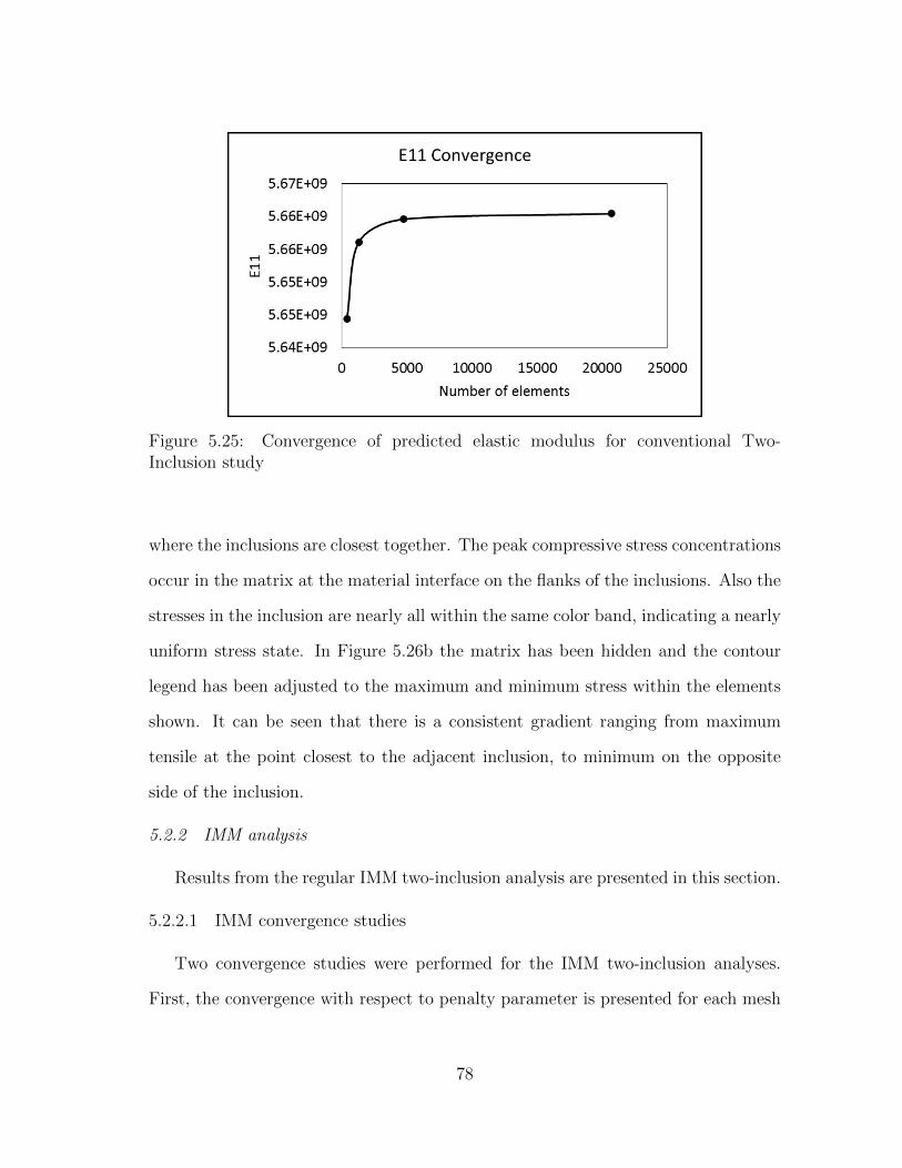
Figure 5.25: Convergence of predicted elastic modulus for conventional Two-Inclusion study
where the inclusions are closest together. The peak compressive stress concentrations
occur in the matrix at the material interface on the flanks of the inclusions. Also the
stresses in the inclusion are nearly all within the same color band, indicating a nearly
uniform stress state. In Figure 5.26b the matrix has been hidden and the contour
legend has been adjusted to the maximum and minimum stress within the elements
shown. It can be seen that there is a consistent gradient ranging from maximum
tensile at the point closest to the adjacent inclusion, to minimum on the opposite
side of the inclusion.
5.2.2 IMM analysis
Results from the regular IMM two-inclusion analysis are presented in this section.
5.2.2.1 IMM convergence studies
Two convergence studies were performed for the IMM two-inclusion analyses.
First, the convergence with respect to penalty parameter is presented for each mesh
78

(a) Global σ11 distribution
(b) Global σ11 distribution in inclu-sion
Figure 5.26: Contour plots of σ11 for coarse conventional mesh
79

refinement. Second, the convergence with respect to mesh refinement for each penalty
parameter is presented. The penalty parameters were varied from slightly below the
suggested value all the way up to values that cause numerical instability in the code.
The penalty values used were [1E10, 1E11, 1E12, 1.052E12, 1E13, 1E16, 1E19, 1E22],
and the meshes used are shown in Figure 5.27.
The convergences of predicted effective modulus for each mesh refinement with
respect to penalty parameter is plotted in Figure 5.28. It can be seen from the
curves that the two less refined meshes do not exhibit the same behavior as the two
more refined meshes. Because of this Mesh 1 and Mesh 2 are not quite converged,
with respect to penalty, until a penalty of 1E16, while the more refined meshes are
converged by the suggested penalty of 1.052E12.
The convergence of predicted effective modulus for each penalty parameter with
respect to mesh refinement is plotted in Figure 5.29. It is evident from these curves,
that the two lowest penalty values are not sufficient. Since the penalty parameter is
analogous to a stiffness coefficient for the bond of the material interface, a value too
low will not impose sufficient displacement compatibility at the material interface
and allow stresses to relax, leading to a lower predicted stiffness. The four highest
penalty values converge to a similar predicted effective modulus.
Key metrics from the convergence study, and their errors relative to the con-
ventional results, are presented in Table 5.6. The values are from the coarse mesh,
Mesh 1, for the suggested and the converged penalty parameters. While the errors
associated with the predicted effective modulus are tolerable, those related to the
peak stresses are significant.
80

(a) Mesh 1 inclusions: 120 elements(b) Mesh 1 matrix: 512 elements (88cut)
(c) Mesh 2 inclusions: 306 elements(d) Mesh 2 matrix: 896 elements(128 cut)
(e) Mesh 3 inclusions: 1122 elements(f) Mesh 3 matrix: 3440 elements(256 cut)
(g) Mesh 4 inclusions: 4672 elements(h) Mesh 4 matrix: 13456 elements(512 cut)
Figure 5.27: Meshes used for IMM Two-Inclusion study
81

Figure 5.28: Convergence of predicted modulus with respect to penalty parameterfor each mesh
Figure 5.29: Convergence of predicted modulus with respect to mesh refinement foreach penalty parameter
Table 5.6: Key metrics from IMM Two-Inclusion analyses
PP Modulus (GPa) Error Peak σ11 (Pa) Error vMax10 σ11 Error
1.052E12 5.6475 0.05 1.6195E8 14.89 0.53 88.481E16 5.7035 1.05 1.7246E8 21.99 0.25 94.57
82

5.2.2.2 Locations of stress concentrations
The locations of stress concentrations within the IMM two-inclusion model are
shown in Figure 5.30, for the suggested penalty parameter, and Figure 5.31, for
the converged penalty value. The contours of the conventional analyses are shown
alongside, and each plot is scaled to the same range as shown. While the contours
of Figure 5.30a and 5.31a seem to exhibit similar characteristics, the contours on the
inclusions alone do not. Figures 5.30d and 5.31d show a stress distribution that is
highly distorted by a failure in the penalty interface connection. Since the boundary
conditions are uniform, and the mesh is identical in the xy plane through the thick-
ness, there is absolutely no reason for there to be any variation of stress through the
thickness. Not only do the stresses from the IMM analyses vary through the thick-
ness of the inclusions, they also have completely erratic distributions throughout the
inclusion.
5.2.3 Simplified case: single material property
The single material property simplification for the two-inclusion model is pre-
sented to show the error that is directly related to the penalty connection between
the master and background meshes. For these analyses, the coarse mesh is used.
After applying a single set of material properties to the entire mesh, those of the tow
in Table 4.1, the conventional analysis predicts an axial elastic modulus of 9.01GPa.
This value is indeed close to the assigned value of E2 (recall the material is aligned
with the first axis out of plane, such that the local y axis is aligned in the global x
direction); it differs slightly due to the restriction of the Poisson contractions in the
boundary conditions.
A penalty-convergence study was performed for the single property IMM analyses
to check for any modified convergence behavior. The convergence of the predicted
83

(a) Conventional (b) IMM
(c) Conventional (d) IMM
Figure 5.30: Contour plots of σ11 for IMM using suggested penalty
(a) Conventional (b) IMM
(c) Conventional (d) IMM
Figure 5.31: Contour plots of σ11 for IMM using converged penalty
84

Figure 5.32: Convergence of single property IMM Two-Inclusion model with respectto penalty parameter
effective modulus is plotted in Figure 5.32. It can be seen that with the modified
material properties, the coarse mesh converges monotonically with respect to penalty
parameter like the two fine meshes did beforehand. This suggests that the irregularity
in the two coarse mesh curves of Figure 5.28 is not solely related to the mesh.
Contour plots of the axial stress for the suggested and converged penalties are
shown in Figure 5.33. In these contour plots, any stress gradient is an error caused
directly by the penalty connection. Both plots of the IMM results contain similar
errors in the matrix elements around the inclusion. The position of these errors,
namely the four corner elements, suggest that the penalty connection does not well
manage X3D8 elements which are heavily intersected by master surfaces.
5.2.4 Simplified case: rotated inclusion
The last results that are presented are for the simplified case where the conven-
tional two-inclusion mesh was modified to be incompatible at the material interface.
By doing this, the penalty connection can be implemented between two incompatibly
85

(a) σ11 using suggested penalty parameter
(b) σ11 using converged penalty parameter
Figure 5.33: Contour plots of σ11 for single property IMM two-inclusion models
86

Figure 5.34: IMM rotated two-inclusion mesh
meshed surfaces without the use of the X3D8 elements.
5.2.4.1 Mesh
The modified two-inclusion mesh was made from the coarse conventional mesh by
slightly rotating the inclusions about the out of plane axis. Since the mesh was ini-
tially compatible, this causes the surface meshes to become incompatible. In addition
since the inclusions are circular, the finite element mesh is a linear approximation
of the circle leading to a faceted perimeter of the inclusion mesh. This is also true
for the cutout in the matrix. Therefore, rotating this faceted surface causes equal
amounts of interpenetration and gaps between the two mesh entities. So, in addition
to rotating the inclusions, their in-plane coordinates were also scaled by a small fac-
tor (in an axisymmetric fashion), to get rid of all of the gaps and increase the size
of the interpenetrations. The resulting modified mesh with the rotated inclusions is
shown in Figure 5.34.
5.2.4.2 Convergence
A convergence study of the predicted effective modulus with respect to penalty
parameter was conducted to evaluate the converged penalty value. The results are
presented in Table 5.7, and the convergence of the predicted modulus is plotted
87

Figure 5.35: Convergence of predicted modulus with respect to penalty parameterfor IMM rotated two-inclusion model
Table 5.7: Key metrics from IMM Rotated model
PP Modulus (GPa) Error Peak σ11 (Pa) Error vMax10 σ11 Error
1.052E12 5.6544 0.18 1.4015E8 0.71 12.34 168.261E16 5.7323 1.56 1.4527E8 2.81 19.62 326.52
in Figure 5.35. The curve of the effective modulus convergence exhibits the same
behavior as in the regular IMM two-inclusion analysis for the coarse mesh.
5.2.4.3 Locations of stress concentrations
The locations of the stress concentrations for the IMM rotated two-inclusion
analysis are shown through the contour plots in Figure 5.36, for the suggested penalty
value, and Figure 5.37, for the converged. In Figure 5.37b and Figure 5.37d it can
be seen that the IMM results match the conventional results extremely well for the
suggested penalty parameter. The peak tensile stress concentration on the inclusion,
labeled A in Figure 5.37d, is slightly larger than in the conventional plot. This
is attributable to the rotation of the inclusion such that there is no longer a node
88

(a) Conventional (b) IMM
(c) Conventional inclusion (d) IMM inclusion
Figure 5.36: Contour plots of σ11 for IMM rotated two-inclusion model using sug-gested penalty
at the point closest to the adjacent inclusion. Rather, there are two nodes spread
equidistantly from this location, causing the peak stress value to be interpolated to
each. This slightly larger concentration is apparent in the higher vMax10 value for the
IMM results, as well as the stress volume distribution curve. The contour plots for
the converged penalty value show that the penalty connection is likely too stiff, given
that there are small interpenetrations in the mesh.
5.2.4.4 Stress volume distributions
The stress volume distributions of σ11 within the matrix and inclusions are plot-
ted for the conventional and IMM rotated two-inclusion models in Figure 5.38 and
Figure 5.39. Like before when the IMM code was updated and the errors were fixed,
the curves in these plots are nearly identical, so they are supplemented with reduced
89

(a) Conventional (b) IMM
(c) Conventional inclusion(d) IMM inclusion
Figure 5.37: Contour plots of σ11 for IMM rotated two-inclusion model using con-verged penalty
range figures. These zoomed in figures are magnified on the top 20% stress values.
The plot for the matrix, Figure 5.38b, show almost identical distributions. The plot
for the inclusion, Figure 5.39b, echoes the contour plot in that a higher amount of
the material gets close to the peak stress.
90

(a) Full range (b) Zoomed in view
Figure 5.38: Volume distributions of σ11 within matrix
(a) Full range (b) Zoomed in view
Figure 5.39: Volume distributions of σ11 within inclusion
91

6. CONCLUSIONS
The objective of this research was to evaluate the performance of the Independent
Mesh Method. This required a suitable strategy for drawing a comparison, which was
addressed by the careful selection and construction of analysis configurations that
required no unnecessary logistical differences between their use in a conventional
analysis and their use in the IMM analysis. Both of the configurations chosen satisfy
this requirement and were proven to produce identical results when the characteristics
of the IMM were not used. In addition, a sufficient set of metrics was required to
evaluate the comparison. The metrics used herein ranged from results such as the
predicted effective elastic modulus, to key stress values such as the peak stresses and
their locations, to very detailed analyses of the distribution of stresses throughout
the material volumes.
It was shown that the initial version of the IMM contained significant coding
issues. These issues were corrected, and the results from the final version of the
IMM code were presented. For the plain weave analysis, the results from the IMM
compared quite well to the conventional benchmark, although there were lingering
differences that were further investigated using the simplified two-inclusion config-
uration. A significant drawback of the IMM is the absence of stress information in
the X3D8 elements, namely the regions of the matrix which interface with the tows.
In textile composites, it is commonly known that when normalized by strength, the
matrix sees the highest normalized stresses. This occurs, of course, at its interfaces
with the volumes occupied by the tows. In its current state, the only accessibility to
this information in an IMM analysis is through interpolation of surrounding results
to points near the matrix-tow interface. The coordinates of these points are not
92

provided, nor are the stresses at the integration points within the X3D8 elements,
so it is impossible to reproduce this information, or use it in post processing.
With the use of the two-inclusion model it was shown that the penalty parameter
has an extreme effect on the results. In addition, the suggested penalty parameter
is not always within the range of converged penalty parameters. Using either the
suggested or the minimum converged penalty value is shown to produce results with
significant distortions in the stress distributions near the material interfaces. The
simplified model using a single material property shows exactly where the locations
that cause these distortions are, although it is difficult to characterize the properties
of the mesh that make these locations different from the others. To this end, the
simplified model using rotated inclusions, without the use of X3D8 elements, provides
insight into what factors are causing the penalty connection to disrupt the stress
fields in the other models. Since the IMM rotated two-inclusion model compares
much better with the conventional than the regular or single property models, it can
be determined that either penalty connections involving X3D8 elements, or penalty
connections involving significantly overlapping elements are the source of the error.
This research has helped to improve the IMM , as well as gain insight into its weak-
nesses, and possible issues. Future work on this subject should involve modification
of the penalty scheme, or perhaps an alternative method for imposing displacement
continuity between the meshes, to remove the errors it is currently causing.
93

REFERENCES
[1] E.G. Zhou, D.H. Mollenhauer, and E.V. Iarve. A realistic 3d textile geometric
model. In Proceedings of 17th International Committee on Composite Materials,
July 2009.
[2] J.D. Whitcomb. Three-dimensional stress analysis of plain weave composites.
Composite Materials Fatigue and Fracture, 3:417–438, 1991.
[3] C.D. Chapman and J.D. Whitcomb. Effect of assumed tow architecture on
predicted moduli and stresses in plain weave composites. Journal of Composite
Materials, 29(16):2134–2159, 1995.
[4] M.K. Ballard, W.R. McLendon, and J.D. Whitcomb. The influence of mi-
crostructure randomness on prediction of fiber properties in composites. Journal
of Composite Materials, 48(29):3605–3620, 2014.
[5] E.G. Zhou, X. Sun, and Y. Wang. Multi-chain digital element analysis in textile
mechanics. Composites Science and Technology, 64:239–244, 2004.
[6] Y. Wang and X. Sun. Digital-element simulation of textile processes. Composites
Science and Technology, 61:311–319, 2001.
[7] E.V. Iarve, D.H. Mollenhauer, E.G. Zhou, T. Breitzman, and T.J. Whitney.
Independent mesh method-based prediction of local and volume average fields
in textile composites. Composites: Part A, 40:1880–1890, 2009.
[8] J.D. Whitcomb, C.D. Chapman, and X. Tang. Derivation of boundary condi-
tions for micromechanics analyses of plain and satin weave composites. Journal
of Composite Materials, 34(9):724–747, 2000.
94

[9] D.M. Blackketter, D.E. Walrath, and A.C. Hansen. Modeling damage in a plain
weave fabric-reinforced composite material. Journal of Composites Technology
& Research, 15(2):136–142, 1993.
[10] J.D. Whitcomb and K. Srirengan. Effect of various approximations on predicted
progressive failure in plain weave composites. Composite Structures, 34:13–20,
1996.
[11] H. Thom. Finite element modeling of plain weave composites. Journal of Com-
posite Materials, 33(16):1491–1510, 1999.
[12] A. Dasgupta, R.K. Agarwal, and S.M. Bhandarkar. Three-dimensional model-
ing of woven-fabric composites for effective thermo-mmechanical and thermal
properties. Composites Science and Technology, 56:209–223, 1996.
[13] V. Carvelli and C. Poggi. A homogenization procedure for the numerical analysis
of woven fabric composites. Composites: Part A, 32:1425–1432, 2001.
[14] X. Tang and J.D. Whitcomb. General techniques for exploiting periodicity
and symmetries in micromechanics analysis of textile composites. Journal of
Composite Materials, 37(13):1167–1189, 2003.
[15] D. Goyal, X. Tang, J.D. Whitcomb, and A.D. Kelkar. Effect of various param-
eters on effective engineering properties of 2 x 2 braided composites. Mechanics
of Advanced Materials and Structures, 12:113–118, 2005.
[16] D. Goyal and J.D. Whitcomb. Analysis of stress concentrations in 2 x 2 braided
composites. Journal of Composite Materials, 40(6):533–546, 2006.
95

[17] K. Woo and J.D. Whitcomb. Three-dimensional failure analysis of plain weave
textile composites using a global/local finite element method. Journal of Com-
posite Materials, 30(9):984–1003, 1996.
[18] K. Woo and J. D. Whitcomb. Macro finite element using subdomain integration.
Communications in Numerical Methods in Engineering, 9:937–949, 1993.
[19] B.N. Cox, W.C. Carter, and N.A. Fleck. A binary model of textile composites-I.
Formulation. Acta Metallurgica et Materialia, 42(10):3463–3479, 1994.
[20] J. Xu, B.N. Cox, M.A. McGlockton, and W.C. Carter. A binary model of textile
composites-II. The elastic regime. Acta Metallurgica et Materialia, 43(9):3511–
3524, 1995.
[21] Q. Yang and B.N. Cox. Spatially averaged local strains in textile composites via
the binary model formulation. Journal of Engineering Materials and Technology,
125:418–425, 2003.
[22] Q.D. Yang and B.N. Cox. Predicting failure in textile composites using the
binary model with gauge-averaging. Engineering Fracture Mechanics, 77:3174–
3189, 2010.
[23] W.G. Jiang, S.R. Hallett, and M.R. Wisnom. Development of domain superpo-
sition technique for the modelling of woven fabric composites. In P.P. Camanho,
C.G. Davila, S.T. Pinho, and J.J.C. Remmers, editors, Mechanical Response of
Composites, chapter 14, pages 281–291. Springer Netherlands, Dordrecht, 2008.
[24] J. Fish, S. Markolefas, R. Guttal, and P. Nayak. On adaptive multilevel su-
perposition of finite element meshes for linear elastostatics. Applied Numerical
Mathematics, 14:135–164, 1994.
96

[25] A.V. Kumar, R. Buria, S. Padmanabhan, and L. Gu. Finite element analysis
using nonconforming mesh. Journal of Computing and Information Science in
Engineering, 8:031005–1–11, 2008.
[26] A.V. Kumar, S. Padmanabhan, and R. Burla. Implicit boundary method for
finite element analysis using non-conforming mesh or grid. International Journal
for Numerical Methods in Engineering, 74:1421–1447, 2008.
[27] S.A. Tabatabaei, S.V. Lomov, and I. Verpoest. Assessment of embedded ele-
ment technique in meso-FE modelling of fibre reinforced composites. Composite
Structures, 107:436–446, 2014.
[28] S.A. Tabatabaei and S.V. Lomov. Eliminating the volume redundancy of em-
bedded elements and yarn interpenetrations in meso-finite element modelling of
textile composites. Computers & Structures, 152:142–154, 2015.
[29] F.T. Peirce. The geometry of cloth structure. Journal of the Textile Institute,
28(3):45–97, 1937.
[30] A. Kemp. An extension of peirce’s cloth geometry to the treatment of non-
circular threads. Journal of the Textile Institute, 49:T44–T48, 1958.
[31] J.W.S. Hearle and W.J. Shanahan. An energy method for calculations in fabric
mechanics part I: Principles of the method. Journal of the Textile Institute,
69(4):81–91, 1978.
[32] J.W.S. Hearle and W.J. Shanahan. An energy method for calculations in fab-
ric mechanics part II: Exampls of application of the method to woven fabrics.
Journal of the Textile Institute, 69(4):92–100, 1978.
97

[33] G. Hivet and P. Boisse. Consistent 3d geometric model of fabric elementary
cell. Application to a meshing preprocessor for 3d finite element analysis. Finite
Element Analysis and Design, 42:25–49, 2005.
[34] F. Robitaille, B.R. Clayton, A.C. Long, B.J. Souter, and C.D. Rudd. Geometric
modelling of industrial preforms: woven and braided textiles. Proceedings of the
Institution of Mechanical Engineers, Part L, 213:69–83, 1999.
[35] F. Robitaille, B.R. Clayton, A.C. Long, B.J. Souter, and C.D. Rudd. Geomet-
ric modelling of industrial preforms: warp-knitted textiles. Proceedings of the
Institution of Mechanical Engineers, Part L, 214:71–90, 2000.
[36] F. Robitaille, A.C. Long, and C.D. Rudd. Geometric modelling of textiles for
prediction of composite processing and performance characteristics. Plastics,
Rubber and Composites, 31(2):66–75, 2002.
[37] F. Robitaille, A.C. Long, I.A. Jones, and C.D. Rudd. Automatically generated
geometric descriptions of textile and composite unit cells. Composites: Part A,
34:303–312, 2003.
[38] H.J. Kim and C.C. Swan. Voxel-based meshing and unit-cell analysis of tex-
tile composites. International Journal for Numerical Methods in Engineering,
56:977–1006, 2003.
[39] H.J. Kim and C.C. Swan. Algorithms for automated meshing and unit cell
analysis of periodic composites with hierarchical tri-quadratic tetrahedral ele-
ments. International Journal for Numerical Methods in Engineering, 58:1683–
1711, 2003.
98

[40] E. Potter, S.T. Pinho, P. Robinson, L. Iannucci, and A.J. McMillan. Mesh
generation and geometrical modelling of 3d woven composites with variable tow
cross-sections. Computational Materials Science, 51:103–111, 2012.
[41] S.K. Boyd and R. Muller. Smooth surface meshing for automated finite element
model generation from 3d image data. Journal of Biomechanics, 39:1287–1295,
2006.
[42] M. Sherburn, A. Long, A. Jones, J. Crookston, and L. Brown. Prediction of
textile geometry using an energy minimization approach. Journal of Industrial
Textiles, 41(4):345–369, 2011.
[43] S.V. Lomov, A.V. Gusakov, G. Huysmans, A. Prodromou, and I. Verpoest.
Textile geometry preprocessor for meso-miechanical models of woven compos-
ites. Composites Science and Technology, 60:2083–2095, 2000.
[44] S.V. Lomov, G. Huysmans, and I. Verpoest. Hierarchy of textile structures and
architecture of fabric geometric models. Textile Research Journal, 71(6):534–
543, 2001.
[45] I. Verpoest and S.V. Lomov. Virtual textile composites software wisetex: Inte-
gration with micro-mechanical, permeability and structural analysis. Composites
Science and Technology, 65:2563–2574, 2005.
[46] S.V. Lomov, D.S. Ivanov, I. Verpoest, M. Zako, T. Kurashiki, H. Nakai, and
S. Hirosawa. Meso-FE modelling of textile composites: Road map, data flow
and algorithms. Composites Science and Technology, 67:1870–1891, 2007.
99

[47] S.V. Lomov, G. Perie, D.S. Ivanov, I. Verpoest, and D. Marsal. Modeling three-
dimensional fabrics and three-dimensional reinforced composites: challenges and
solutions. Textile Research Journal, 81(1):28–41, 2011.
[48] S.V. Lomov, I. Verpoest, J. Cichosz, C. Hahn, D.S. Ivanov, and B. Verleye.
Meso-level textile composites simulations: open data exchange and scripting.
Journal of Composite Materials, 48(5):621–637, 2014.
[49] F. Desplentere, S.V. Lomov, D.L. Woerdeman, I. Verpoest, M. Wevers, and
A. Bogdanovich. Micro-CT characterization of variability in 3d textile architec-
ture. Composites Science and Technology, 65:1920–1930, 2005.
[50] A. Drach, B. Drach, and I. Tsukrov. Processing of fiber architecture data for
finite element modeling of 3d woven composites. Advances in Engineering Soft-
ware, 72:18–27, 2014.
[51] G. Grail, M. Hirsekorn, A. Wendling, G. Hivet, and R. Hanbli. Consistent finite
element mesh generation for meso-scale modeling of textile composites with
preformed and compacted reinforcements. Composites: Part A, 55:143–151,
2013.
100