NeuroImage 54 (2011) S165–S175

Contents lists available at ScienceDirect

NeuroImage

j ourna l homepage: www.e lsev ie r.com/ locate /yn img

Evaluation of fiber bundles across subjects through brain mapping and registration ofdiffusion tensor data

Darshan Pai a, Hamid Soltanian-Zadeh b,c,⁎, Jing Hua a

a Department of Computer Science, Wayne State University, Detroit, MI, USAb Image Analysis Laboratory, Radiology Department, Henry Ford Health System, Detroit, MI, USAc Control and Intelligent Processing Center of Excellence (CIPCE), School of Electrical and Computer Engineering, University of Tehran, Tehran, Iran

⁎ Corresponding author. Radiology Image Analysis LaOne Ford Place, 2F, Detroit, MI 48202, USA. Fax: +1 31

E-mail address: hamids@rad.hfh.edu (H. Soltanian-Z

1053-8119/$ – see front matter © 2010 Elsevier Inc. Aldoi:10.1016/j.neuroimage.2010.05.085

a b s t r a c t

a r t i c l e i n f o

Article history:Received 5 December 2009Revised 6 May 2010Accepted 29 May 2010Available online 12 June 2010

Keywords:Analysis of fiber bundlesDiffusion imagingEpilepsyShape analysisMultimodality fusionMedical image processing

This paper presents a visualization and analysis framework for evaluating changes in structural organizationof fiber bundles in human brain white matter. Statistical analysis of fiber bundle organization is conductedusing an anisotropy measure, volume ratio (VR), which is ratio of anisotropic and isotropic components.Initially fiber bundles are tracked using a probabilistic algorithm starting from seed voxels. To ensureaccurate selection of seed voxels and to prevent operator bias, a reference brain (MNI_152) is used whenmarking ROIs. Individual structural MRI brain scans are mapped to the reference using volumetric conformalparameterization. This mapping preserves topology and aligns features perfectly making it a robust andaccurate registration technique. One-to-one mapping to the template allows ROI selection and subsequenttransfer of ROI to structural MRI of subject. Affine registration coregisters structural MRI and DTI. Seed voxelsare mapped to DTI using the resulting transformation parameters. To evaluate the proposed approach, MRIand DTI of 12 normal volunteers and 15 medial temporal lobe epilepsy patients are used. First, a statisticalhypothesis testing is conducted to test for anisotropy changes in cingulum and fornix fiber bundles ofepileptic patients. Experimental results reveal a 40% decrease in anisotropy levels of cingulum in patientscompared to volunteers. They also show a 25% overall decrease in anisotropy of fornix. Secondly, shapes ofthe bundles are visualized in 3D illustrating that the bundles of epileptic patients are bumpy while those ofnormal volunteers are smooth.

b., Henry Ford Health System,3 874 4494.adeh).

l rights reserved.

© 2010 Elsevier Inc. All rights reserved.

Introduction

The advent of high-end and computationally intensive machineshas improved the acquisition of various 3-D neuroimaging data. Thecomplexity, scale, and resolution of the images have increasedsignificantly in recent years. As a result, huge amount of data isavailable for analysis. Different imaging modalities provide comple-mentary information regarding the anatomy, physiology, and struc-ture of the living organs and tissues. They include anatomical anddiffusion data provided by magnetic resonance imaging (MRI) anddiffusion tensor imaging (DTI); molecular imaging and functional dataprovided by positron emission tomography (PET) and functional MRI(fMRI); and electrophysiological data provided by electroencepha-lography (EEG). Normal brain function is characterized by variousinteractions between specific regions of the brain. A frameworkcombining the various facets of the anatomy and physiology of thehuman brain is a requirement for a robust pathological analysis. Wepresent a framework for evaluation of the fiber bundles based on two

modalities, MRI and DTI, which together provide an excellentrepresentation of the white matter organization as well as changesassociated with disease.

Statistical analysis (Miller et al., 1997; Styner et al., 2003;Thompson and Toga, 2002) in brain abnormality studies are typicallypopulation-based comparisons that reveal significant differencesbetween healthy volunteers and patients. The results can help achieveimportant objectives in many neuroscience studies, for instance,delineating the anatomical region affected by disease facilitates futurecourse of treatment and surgical planning. Given the complexanatomy of the brain, a robust registration strategy is required foraccurate alignment of inter-subject brain images. An accuratedepiction of normal anatomical variability in specific regions acrosssubjects depends on the homology between them. In recent years,various brain mapping algorithms have been developed (Miller et al.,1997; Styner and Gerig, 2001; Thompson et al., 2001) to address thisdependency and to allow an accurate statistical analysis. Mappingalgorithms can be classified into two categories: implicit imageintensity-based technique; and explicit computational geometry-based technique. The intensity-based technique does not requiresegmentation of the brain structures (regions). It uses an implicitcharacterization based on intensity distributions. This facilitates

S166 D. Pai et al. / NeuroImage 54 (2011) S165–S175

voxel-based analysis and not a surface-based analysis (Muzik et al.,2007; Friston et al., 1994; Muzik et al., 2000). The geometry-basedtechnique takes advantage of additional explicit geometric propertiesof the brain structures and achieves accurate mapping and registra-tion of the brain images permitting surface-based analysis. Freesurfer(Fischl et al., 1999) and Caret (Essen et al., 2001) are popular methodsthat combine the geometry with automatic anatomical labelingmethods to achieve a powerful representation for analyzing corticalbrain structures. Since geometry is an important aspect, pre-processing is a required first step. Various representations havebeen proposed for surface analysis. They include curvature-basedrepresentations (Vemuri et al., 1986), regional point representations(Chua and Jarvis, 1997), spherical harmonics (Kazhdan et al., 2003),shape distributions (Osada et al., 2002), spline representations(Camion and Younes, 2001), and harmonic shape images (Zhang,1999). These methods, however, suffer from mismatches due toinsufficient discriminative power. Riemannian geometry has a distinctadvantage since it is based on intrinsic geometric properties of themanifold and corrects for this mismatch (Drury, 1999; Wang et al.,2005). Conformal mapping based on the harmonic energy minimiza-tion on a 2D manifold allows for accurate registration in genus zerosurfaces, which is topologically equivalent to the cortical brainsurface. This technique has been extended to 3D manifolds forvolumetric mapping and analysis (Wang et al., 2004). Moreover, themapping is bijective and is easily transferred to the native space of thesubject. In this paper, we present a constrained conformal mappingapproach for matching structural MRI images.

DTI is the preferred modality for visualizing the structuralorganization of the white matter microstructure. The anisotropicproperties and directional diffusivity obtained from the DTI tensor ateach voxel is used to analyze and detect white matter abnormalities.Statistical analysis and matching, however, is not straightforward inDTI mainly due to the orientation information inherent in the data.Spatial Normalization (Park et al., 2003; Jones et al., 2002) of the DTIbrain dataset, for quantification of diffusion tensor differencesbetween populations, were conducted with unsatisfactory resultsbecause only intensity was considered (Wakana et al., 2004). TheTract-Based Spatial Statistics (TBSS) method (Smith et al., 2006)improves on this by using skeletonization to normalize the fractionalanisotropy (FA) images which measures the voxel-based statisticsalongmajor fiber tracts. In general, spatial normalization is non-trivialand can modify the real tensor orientation of the underlying data(Alexander et al., 2001). It can potentially modify abnormalitiescaptured in the native space, for instance, structural changes in thefiber tracts.

The most popular method to identify changes in the structuralorganization of the white matter fibers is tractography, which ischaracterized as deterministic fiber tracking and probabilistic fibertracking. Deterministic fiber tracking tracks single-fiber populations(Parker, 2000; Hagmann, 2004; Mori et al., 1999; Frank 2001) byfollowing the direction of the major eigen-vector of the tensorellipsoid at each voxel. Major eigen-vectors are well-defined at placeswhere the anisotropy is high and the tracts are reliable only for linearanisotropy diffusion profiles. Probabilistic tracking improves on thisdisadvantage by introducing uncertainty in the tracking algorithm forestimating the fiber directions. Consequently, the algorithm allowstracking in hard to reach areas (Brehens et al., 2003; Friman et al.,2006). Since the tracks do not represent real fiber orientationsbecause of the random sampling criteria, we rely on the connectivitystrength prediction between voxels to describe a global probabilityconnectivity map. Various methods for computing this connectivityemploy techniques that achieve a greedy or global optimum and havebeen studied extensively.

In this paper, we concentrate on using anisotropy markers formeasuring tract integrity. Our hypothesis testing studies rely on thevolume ratio (VR) to characterize structural changes in white matter

fiber bundles. This hypothesis is evaluated bymeasuring white matterdifferences in the fornix and the cingulum fiber bundles of medialtemporal lobe epilepsy patients. MRI brain scans of individual subjectsare parameterized onto a curvature-constant volume representing thecanonical domain for mapping. Additionally, the anatomical anddiffusion images of the same subject are registered using an affineregistration algorithm. Since these mappings are bijective, thestatistical results can be generated in the native space of the DTIimage. The regions of interests (ROIs) that define the seed voxels fortracking are chosen on the template and transformed to the native DTIspace of the subject using the transformation parameters obtainedduring registration. The final results show that anisotropy differencesin the fiber bundles measured using the mean VR is significantbetween the patient and the normal groups. Moreover, we employ aregion-growing algorithm to determine the shapes of these bundlesproviding a visual interface to identify shape changes associated withdisease. The method and the results are explained in detail in thefollowing sections.

Materials and methods

Subjects and imaging data

The MRI and DTI data of fifteen medial temporal lobe epilepsypatients (10 males, 5 females, ages 43±16) and twelve normalvolunteers (9 males, 3 females, ages 32±5) enrolled in researchstudies approved by the IRB committee of Henry Ford Hospital,Detroit, Michigan, USA were used in this work. All imaging data wereacquired on a 3 Tesla GE Signa system (General Electric, Milwaukee,WI, USA) at Henry Ford Hospital, Detroit, Michigan, USA. The imagingprotocol included anatomical T1-weighted images and diffusiontensor images. The T1-weighted images were acquired in the coronalplane using a 3D inversion recovery (IR) spoiled gradient-echo (SPGR)sequence with TR/TI/TE=7.6/1.7/500 ms, flip angle=20°, field ofview (FOV)=200 mm×200 mm, matrix size=256×256, pixelsize=0.781 mm×0.781 mm, and slice thickness=2.0 mm. The DTIdata were acquired in the axial plane using 25 non-collinearweighting directions and a single shot echo planar imaging (EPI)sequence with a b-value of 1000 s/mm2. Each volume covered a240 mm×240 mm field of view with 0.9375 mm×0.9375 mm in-plane resolution and 2.6 mm slice thickness with no inter-slice gap.

Conformal mapping

Conformal parameterization of the 3D-representative geometry inthe 2D space is a preferable choice since it simplifies computationalcomplexity. Gu et al. (2004) described a harmonic energy minimiza-tion algorithm for generating a conformal map between genus zerosurfaces and a canonical surface (sphere). The canonical domain iscurvature-constant, which eliminates problems associated withdistance fields in the Euclidian space. Moreover, matching corticalpatterns in the canonical domain becomes highly efficient.

We represent our standardized space as canonical domainstructures of closed genus zero topology and term it as the ConformalBrain Model (CBM). A genus zero topology is a geometric structurewith no holes. For statistical analysis, a representative brain is neededwhich will be the template for matching. This model can be one of thedatasets used for analysis or an average brain representation from atraining set of normal subject brains. We chose the MNI_152 atlasbrain as our reference template for analysis and the correspondingmap will be the template CBM. The following paragraph explains themethod to compute the template CBM.

Initially, we concentrate on the conformal mapping of the braincortical surface. The brain cortical surface can be viewed as a closedgenus zero surface that can be parameterized in the spherical domain.The mapping is defined using the function f:S2→R3, where f is a vector

S167D. Pai et al. / NeuroImage 54 (2011) S165–S175

valued function that maps the coordinates of the sphere in sphericalcoordinates onto the cortical brain surface. Fig. 1 provides a goodillustration for the conformal mapping. Consider two surfacesM andNwith a conformal mapping ϕ between them. If γ1and γ2 are twocurves defined on M with an intersecting angle α, then the cor-responding curves ϕ(γ1) and ϕ(γ2) defined on N will intersect at thesame angle α. This is demonstrated by the checkerboard pattern onthe surfaces shown in Fig. 1 illustrating that the angles are preserved.For the function f:M→N defined above, the mapping can be madeconformal by minimizing the harmonic energy of the map (Gu et al.,2004). Genus zero surfaces are defined by meshes. For a simplicialcomplex |K|, and the map f, the implicit energy is defined by

E = ∑u;v∈k

ku;v‖ f ðuÞ−f ðvÞ‖2; ð1Þ

where u and v denote vertices, {u,v} denotes the edge linking u and v,and ku,v is a constant representing the string energy between u and v.Since f represents a vector valued function,

→f = f f0; f1; f2g, defined

over |K|, the energy of f is computed by

E→f

� �= ∑

2

i=0Eð fiÞ: ð2Þ

The function f is harmonic if and only if the Laplacian of f in thetangential direction is zero. This can be easily solved using thesteepest descent algorithm of the form

d→f ðtÞdt

= −Δ→f ðtÞ; ð3Þ

such that the string energy is minimized. This map is conformal andrepresents a smooth and angle-preservingmapping from a genus zerosurface M, representing the brain surface, to a unit canonical sphereS2. The conformal factor e2λ and the mean curvature on the surfaceh are treated as functions on the sphere. These functions completelydefine the surface S2 uniquely except for a rigid rotation (Gu et al.,2004). A Cartesian coordinate system is defined which specifies a 3Drotation transformation to guarantee a unique orientation of thesphere (Zou et al., 2006). Note that this mapping is only a partial stepfor creating the template CBM.

Volumetric conformal mapping

In the volumetric case, the brain volume is represented by thetetrahedral mesh. We keep the same genus zero requirements thatwill now map the tetrahedral mesh to a solid ball. The tetrahedralmesh of a brain is shown in Fig. 2a. Fig. 2b shows the left-hemisphere

Fig. 1. An illustration of conformal mapping where the angles of the squares in thecheckerboard pattern are preserved.

highlighting the internal structures. The procedure to create thetemplate CBM is exactly the same as before. The surface map is fixedand the algorithm proceeds to minimize the harmonic energy of theinternal structures. This step is computationally intensive because ofthe increased resolution. The algorithm computes the template CBMas shown in Fig. 2d. The template CBM represents the canonical spacefor brain mapping. The volumetric conformal map also preserves thegeometry between the two volumes. A textured slice shown in the cutsection of the sphere (Figs. 2e–f) highlights the fact that the geometryis preserved during mapping.

Brain volume matching using CBM-landmark-constrained shapeoptimization

The CBM provides a 3D-representation of the brain volumegeometry in the canonical domain. For cross-subject analysis, theCBM should be homologous across all datasets. This cannot beachieved with conformal mapping alone and alignment between itsvarious anatomical features is important. Features are sulcal land-marks and internal subcortical structures most common across brainpopulations. These include cortical patterns, such as the ones shownin Figs. 3c and 4a and internal brain structures (Fig. 3a) like the corpuscallosum, pons, anterior commissure, and cingulate. Structural MRIeffectively delineates these features and is the preferred modality foralignment. An expert neuroanatomist selects the features for all theindividual MRI scans under study. A well-balanced set of featuresacross the brain guarantees the accuracy of the alignment. Some of thesurface landmarks shown in Fig. 4 are central sulcus, pre-centralsulcus, post-central sulcus, superior frontal sulcus, sylvian fissure,superior temporal sulcus, inferior temporal sulcus, parieto-occipital,and transverse occipital sulcus. Internal landmarks are edges andpoints, the AC–PC line, and edges of well-known structures internal tothe brain. The landmarks are chosen as a set of ordered point's {Pi}across the brain volume. Conformal mapping to the template CBMorients the brain volumes while the landmark constraints minimizethe inherent variability in the anatomical domain and matches twoCBMs perfectly.

Various ideas has been proposed (Gu et al., 2004; Wang et al.,2005) tackling this issue. A landmark-constrained conformal mapping(Zou et al., 2006) is described below. Given a set of point's {Pi}representing the landmarks, conformal mapping is employed on atemplate brain without any landmark constraints. The MNI_152 brainatlas, a standard averaged brain from a database of 152 normalsubjects (Fig. 4a), is mapped to the spherical domain and theharmonic energy minimization on the surface and the subsequentminimization on the volume computes the conformal model termedthe template CBM (Fig. 4b). Fig. 4 illustrates the steps of the matchingprocess. Fig. 4b shows the template CBM with the landmarks {pi∈C1}defined on it. For an individual subject, we assume initially that thelandmarks are very close to the ones defined on the template {qi∈C2}.The initial mapping of the subject onto the sphere is shown in Fig. 4c.The set of ordered points is ensured to have the same cardinality. Alandmark-constrained optimization is computed using the steepestdescent algorithm as described in the previous section. This procedurestill minimizes the harmonic energy but every ordered point {pi} isconstrained to be aligned with its counterpart {qi} on the template.The next step is to align the brain regions between the landmarks. Thisis achieved by matching the anatomical shapes using a distancefunction in the shape space given as

dðS1; S2Þ = ∫vððλ1−λ2Þ2 + ðh1−h2Þ2Þdμ ð4Þ

where S1=(λ1, h1) and S2=(λ2, h2) and dμ is the volume element onthe sphere. S1 and S2 are the two spherical volumes to be matched andλ and h are the conformal factor and the mean curvature, respectivelydefined as functions on the sphere that determine the spherical map

Fig. 2. An illustration of conformal mapping applied to brain: (a) tetrahedral mesh equivalent of the brain volume; (b) internal mesh structure; (d) the solid ball created byvolumetric conformal mapping; (e) internal structure of the brain after the conformal mapping; (c), (f) interpolated slices which show that the conformal mapping preserves thebrain geometry.

S168 D. Pai et al. / NeuroImage 54 (2011) S165–S175

unique up to rigid motions in R3. This optimization determines theoptimal shape transformation functional that minimizes the distancefield between the two shapes. To ensure that the optimization isstable and also to use well-known features that are stable across thedatasets, very coarse smoothing is allowed on the brain surface.Fig. 4d shows the subject brain CBM aligned to the template CBM.

Affine registration

The conformal mapping is invertible and has a one-to-onemapping between individual MRIs and the template. The templatewill be used for choosing ROIs and other functional elements or areas.The ROIs for seeding the voxels for fiber tracking is chosen on thetemplate. Through affine registration, the voxels are mapped onto theindividual DTI scans for tracking. We argued before on the potentialproblems associated with spatial normalization of the DTI, whichaffects the tensor orientation. Hence, instead of warping the DTI to theMRI, the registration parameters are saved. We choose the non-diffusion weighted image, i.e., the image with no diffusion gradient(b=0), and register it to the MRI using 12-parameter affineregistration. Combining the affine transformation parameters withthe conformal map creates the transformation space necessary toconvert the voxels selected on the template down to each individual

Fig. 3. A sagittal slice (a) and a surface view (b) of the brain that may be used to select the lan

DTI image. This is advantageous since the same ROIs are seeded acrossall the subjects preventing bias. The ROIs will represent the samespatial region across the subject populations. Affine image registrationis available in the well-known packages like FSL (Brehens et al., 2003),AIR (Woods et al., 1998), and SPM.

Probabilistic fiber tracking

Thefinal step is to generate quantitativemeasures for the statisticalanalysis study. For anisotropy analysis, we track the neural fibers fromthe DTI data.We briefly describe the underlyingmodel of the diffusiontensor image. Diffusion MRI is a relatively new modality and relatesdisplacements of water molecules, p, in the tissue with the imageintensities.Whitematter tissue in the humanbrain contains bundles ofneural fibers connecting various functional areas. For brain images, p,along these fiber directions is higher. Hence, the probability distribu-tion of p represents a cigar shaped structure (Fig. 5c) indicating highanisotropy. Diffusion tensor MRI (DT-MRI) models p as a simplediffusion with a Gaussian profile given by

Gðx;D; tÞ = ðð4πtÞ3 detðDÞÞ−1=2 exp−xTD−1x

4t

!; ð5Þ

dmarks in comparison to an atlas (c) that shows various landmarks on the brain surface.

Fig. 4. The MNI 152 atlas (a) and the template CBM (b). Matching the features in (b) to a CBM of an individual (c) generates an optimized landmark-constrained version (d).

S169D. Pai et al. / NeuroImage 54 (2011) S165–S175

where D is the diffusion tensor and t is the diffusion time. The MRIacquisition sequences follow the Stejskal–Tanner imaging sequence(Stejskal and Tanner, 1965), which models the observed intensity ofanisotropic samples as

S = S0e−bgtDg

; ð6Þ

where b defines a parameter of the sequence called the weightingfactor. To sample the ellipsoid uniquely, the 3×3 diffusion tensor Dneeds to be solved. This requires at least six independent measure-ments along different gradient orientations g. The principal directionsof the tensor at each voxel are calculated using singular valuedecomposition. The eigen-values specify an orientation-independentmeasure of the anisotropy at each voxel and the corresponding eigen-vectors specify the directions of water diffusion. Reconstructing thewhite matter pathways from principal directions provide a means forassessing pathological changes in the white matter. We describe twomethods to track these pathways.

Deterministic tracking tracks fibers along the primary eigen-direction e1 at each voxel. Many fiber bundles have been reliablytracked by this method and validated. The single direction criterionfor tractographymakes it difficult to track in areas where the diffusionis more isotropic, for instance, complex fiber neighborhoods(λ1≈λ2≫λ3) that correspond to multi-fiber orientation within avoxel, resulting in unreliable tracking results (see Fig. 5). To overcomethese limitations, a probabilistic tracking algorithm is devised. Wefollow the algorithm derived by Friman et al. (2006) in his paper. Thealgorithm is based on a Bayesian inference and estimation scheme.Uncertainties, due to noise or complex fiber architectures, are notdisregarded but captured in the model itself in the form of theposterior distribution at each voxel. Given a source region A, theprobability of connectivity between A and a target region B is given by

pðA→B jDÞ = ∑∞

n=1∫Ωn

ABpðnÞpðv1:n jDÞ; ð7Þ

where p(v1:n|D) is the probability of the fiber path going from A to Bgiven the diffusion data D and ΩAB

n represents the sampling space of

Fig. 5. (a) Isotropic profile (λ1≈λ2≈λ3). (b) Ellipsoidal profile (λ1Nλ2≈λ3). (c) Highly anishown in each case where e1 is the primary eigen-direction.

the connectivity between A and B of path length 1 through n. SinceEq. (7) is not analytically solvable, a rejection sampling strategy isemployed. A large number of sampled fiber paths starting from thesource region A are drawn at random and the probabilities of thepaths between A and B are evaluated. Each random path is evaluatedlocally in steps up until the predetermined length n. The steps areassumed to be unit length vectors, with the condition that each stepdepends only on the previous step. Since these samples reflect themodel of the actual fibers, the posterior distribution at each step iscalculated based on the diffusion data D at that voxel. This distributionbased on the Bayes theorem is written as

pðv̂i; θ jv̂i−1;DÞ =pðD jv̂i; θÞpðv̂i jv̂i−1ÞpðθÞ

pðDÞ : ð8Þ

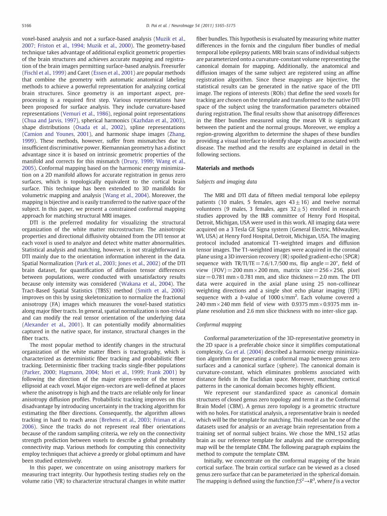
The first term in the numerator is the likelihood at the current stepand uses a constrained model based on a Gaussian diffusion profile.pðv̂i jv̂i−1Þ is the prior to indicate the dependence of the current step onthe previous step. This assumption works well in a complex fiberneighborhood because there will always be a preference on theprevious step. The nuisance priors, p(θ), address the parameters of theGaussian profile modeled as dirac priors. As explained by Friman et al.(2006), using dirac priors significantly saves computation time.Finally, p(D) is a normalizing constant that gives the probabilitydistribution at v̂i distributed over a unit sphere as shown in Fig. 6a. Todraw a random path, the sphere is discretized uniformly into a finiteset of unit vectors indicating possible directions. The next stepdirection is picked at random and added to the path. The fiber pathsrepresent the sampling space of the source region. The fiber paths areillustrated in Fig. 6b.

Shape analysis of fiber bundles

Anisotropic differences are indicative of the changes in thestructural organization of the fiber bundle. Abnormalities associatedwith changes in anisotropy can be visually inferred from the fiberbundle shape. We can quantify the shape differences using well-knownmeasures such as curvature. Many researchers have presented

sotropic cigar-shaped profile (λ1≫λ2 and λ1≫λ3). The eigen-vectors (directions) are

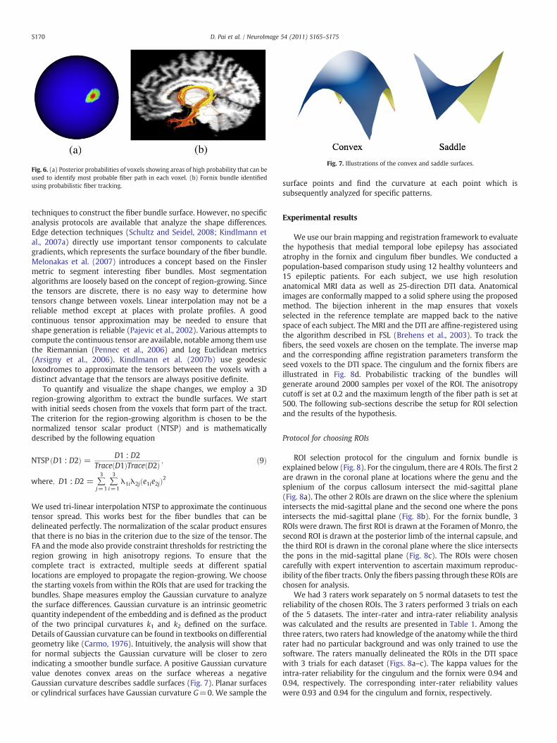
Fig. 6. (a) Posterior probabilities of voxels showing areas of high probability that can beused to identify most probable fiber path in each voxel. (b) Fornix bundle identifiedusing probabilistic fiber tracking.

Fig. 7. Illustrations of the convex and saddle surfaces.

S170 D. Pai et al. / NeuroImage 54 (2011) S165–S175

techniques to construct the fiber bundle surface. However, no specificanalysis protocols are available that analyze the shape differences.Edge detection techniques (Schultz and Seidel, 2008; Kindlmann etal., 2007a) directly use important tensor components to calculategradients, which represents the surface boundary of the fiber bundle.Melonakas et al. (2007) introduces a concept based on the Finslermetric to segment interesting fiber bundles. Most segmentationalgorithms are loosely based on the concept of region-growing. Sincethe tensors are discrete, there is no easy way to determine howtensors change between voxels. Linear interpolation may not be areliable method except at places with prolate profiles. A goodcontinuous tensor approximation may be needed to ensure thatshape generation is reliable (Pajevic et al., 2002). Various attempts tocompute the continuous tensor are available, notable among them usethe Riemannian (Pennec et al., 2006) and Log Euclidean metrics(Arsigny et al., 2006). Kindlmann et al. (2007b) use geodesicloxodromes to approximate the tensors between the voxels with adistinct advantage that the tensors are always positive definite.

To quantify and visualize the shape changes, we employ a 3Dregion-growing algorithm to extract the bundle surfaces. We startwith initial seeds chosen from the voxels that form part of the tract.The criterion for the region-growing algorithm is chosen to be thenormalized tensor scalar product (NTSP) and is mathematicallydescribed by the following equation

NTSP ðD1 : D2Þ = D1 : D2TraceðD1ÞTraceðD2Þ ;

where; D1 : D2 = ∑3

j=1∑3

i=1λ1iλ2jðe1ie2jÞ2

ð9Þ

We used tri-linear interpolation NTSP to approximate the continuoustensor spread. This works best for the fiber bundles that can bedelineated perfectly. The normalization of the scalar product ensuresthat there is no bias in the criterion due to the size of the tensor. TheFA and the mode also provide constraint thresholds for restricting theregion growing in high anisotropy regions. To ensure that thecomplete tract is extracted, multiple seeds at different spatiallocations are employed to propagate the region-growing. We choosethe starting voxels from within the ROIs that are used for tracking thebundles. Shape measures employ the Gaussian curvature to analyzethe surface differences. Gaussian curvature is an intrinsic geometricquantity independent of the embedding and is defined as the productof the two principal curvatures k1 and k2 defined on the surface.Details of Gaussian curvature can be found in textbooks on differentialgeometry like (Carmo, 1976). Intuitively, the analysis will show thatfor normal subjects the Gaussian curvature will be closer to zeroindicating a smoother bundle surface. A positive Gaussian curvaturevalue denotes convex areas on the surface whereas a negativeGaussian curvature describes saddle surfaces (Fig. 7). Planar surfacesor cylindrical surfaces have Gaussian curvature G=0. We sample the

surface points and find the curvature at each point which issubsequently analyzed for specific patterns.

Experimental results

We use our brain mapping and registration framework to evaluatethe hypothesis that medial temporal lobe epilepsy has associatedatrophy in the fornix and cingulum fiber bundles. We conducted apopulation-based comparison study using 12 healthy volunteers and15 epileptic patients. For each subject, we use high resolutionanatomical MRI data as well as 25-direction DTI data. Anatomicalimages are conformally mapped to a solid sphere using the proposedmethod. The bijection inherent in the map ensures that voxelsselected in the reference template are mapped back to the nativespace of each subject. The MRI and the DTI are affine-registered usingthe algorithm described in FSL (Brehens et al., 2003). To track thefibers, the seed voxels are chosen on the template. The inverse mapand the corresponding affine registration parameters transform theseed voxels to the DTI space. The cingulum and the fornix fibers areillustrated in Fig. 8d. Probabilistic tracking of the bundles willgenerate around 2000 samples per voxel of the ROI. The anisotropycutoff is set at 0.2 and the maximum length of the fiber path is set at500. The following sub-sections describe the setup for ROI selectionand the results of the hypothesis.

Protocol for choosing ROIs

ROI selection protocol for the cingulum and fornix bundle isexplained below (Fig. 8). For the cingulum, there are 4 ROIs. The first 2are drawn in the coronal plane at locations where the genu and thesplenium of the corpus callosum intersect the mid-sagittal plane(Fig. 8a). The other 2 ROIs are drawn on the slice where the spleniumintersects the mid-sagittal plane and the second one where the ponsintersects the mid-sagittal plane (Fig. 8b). For the fornix bundle, 3ROIs were drawn. The first ROI is drawn at the Foramen of Monro, thesecond ROI is drawn at the posterior limb of the internal capsule, andthe third ROI is drawn in the coronal plane where the slice intersectsthe pons in the mid-sagittal plane (Fig. 8c). The ROIs were chosencarefully with expert intervention to ascertain maximum reproduc-ibility of the fiber tracts. Only the fibers passing through these ROIs arechosen for analysis.

We had 3 raters work separately on 5 normal datasets to test thereliability of the chosen ROIs. The 3 raters performed 3 trials on eachof the 5 datasets. The inter-rater and intra-rater reliability analysiswas calculated and the results are presented in Table 1. Among thethree raters, two raters had knowledge of the anatomywhile the thirdrater had no particular background and was only trained to use thesoftware. The raters manually delineated the ROIs in the DTI spacewith 3 trials for each dataset (Figs. 8a–c). The kappa values for theintra-rater reliability for the cingulum and the fornix were 0.94 and0.94, respectively. The corresponding inter-rater reliability valueswere 0.93 and 0.94 for the cingulum and fornix, respectively.

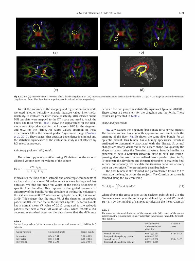
Fig. 8. (a) and (b) show the manual selection of ROIs for the cingulum in DTI. (c) shows manual selection of the ROIs for the fornix in DTI. (d) A DTI image on which the extractedcingulum and fornix fiber bundles are superimposed in red and yellow, respectively.

Table 2The mean and standard deviations of the volume ratio (VR) values of the normal

S171D. Pai et al. / NeuroImage 54 (2011) S165–S175

To test the accuracy of the mapping and registration framework,we used another reliability analysis measure called inter-modalreliability. To evaluate the inter-modal reliability, ROIs selected on theMRI template were mapped to the DTI space and used to track thefibers. The third row in Table 1 shows the kappa values for the inter-modal reliability calculated for the 5 datasets, 0.85 for the cingulumand 0.92 for the fornix. All kappa values obtained in theseexperiments fell in the “almost perfect” agreement range (Pantaziset al., 2010). They suggest that operator dependence is minimal andthe statistical significance of the evaluation study is not affected byROI selection protocol.

Anisotropy (volume ratio) results

The anisotropy was quantified using VR defined as the ratio ofellipsoid volume over the volume of the sphere

VR = 1− 27λ1λ2λ3

ðλ1 + λ2 + λ3Þ3: ð10Þ

It measures the ratio of the isotropic and anisotropic components ateach voxel so that a lower VR value indicates more isotropy and lessdiffusion. We find the mean VR values of the voxels belonging tospecific fiber bundles. This represents the global measure ofanisotropy of the bundle. For the cingulum of the healthy volunteers,this value is around 0.187 whereas for epileptic patients, it is around0.109. This suggest that the mean VR of the cingulum in epilepticpatients is 40% less than that of the normal subjects. The fornix bundlehas a normal mean VR value of 0.212 compared to the epilepticpatients that have a mean VR value of 0.159, which reflects a 25%decrease. A standard t-test on the data shows that the difference

Table 1Average kappa values (κ) for intra-rater, inter-rater, and inter-modal reliability for 5datasets.

Kappa values (κ) Cingulum bundle Fornix bundle

Intra-rater 0.94±0.04 0.94±0.03Inter-rater 0.93±0.04 0.94±0.04Inter-modal 0.85±0.02 0.92±0.04

between the two groups is statistically significant (p-valueb0.0001).These values are consistent for the cingulum and the fornix. Theseresults are presented in Table 2.

Shape analysis results

Fig. 9a visualizes the cingulum fiber bundle for a normal subject.The bundle surface has a smooth appearance consistent with theanatomy of the fiber. Fig. 9b shows the same fiber bundle for anepileptic patient. This bundle has a bumpy appearance, which isattributed to abnormality associated with the disease. Structuralchanges are clearly visualized in the surface shape. We quantify theshape variations using the Gaussian curvature. Smooth bundles areexpected to have a Gaussian curvature close to zero. The region-growing algorithm uses the normalized tensor product given in Eq.(9) to create the 3D volume and the marching cubes to create the finalsurface. Subsequently, we calculate the Gaussian curvature at everypoint on the surface. The procedure is described below.

The fiber bundle is skeletonized and parameterized from 0 to t tonormalize the lengths across the subjects. The Gaussian curvature issampled along the skeleton using

Cðr; θ; tÞ = ∫∫Gðr; θ; tÞdrdθdt; ð11Þ

where drdθ is the cross-section at the skeleton point dt and G is theGaussian curvature at the surface point defined by r and θ. We divideEq. (11) by the number of samples to calculate the mean Gaussian

subjects and the temporal lobe epilepsy patients in the cingulum (a) and the fornix (b)fiber bundles.

Mean volumeratio±standarddeviation

p-value oft-test

Normal subjectsa 0.187±0.031 3.74×E−06Temporal lobe epilepsy patientsa 0.109±0.012Normal subjectsb 0.212±0.030 9.20×E−05Temporal lobe epilepsy patientsb 0.159±0.015

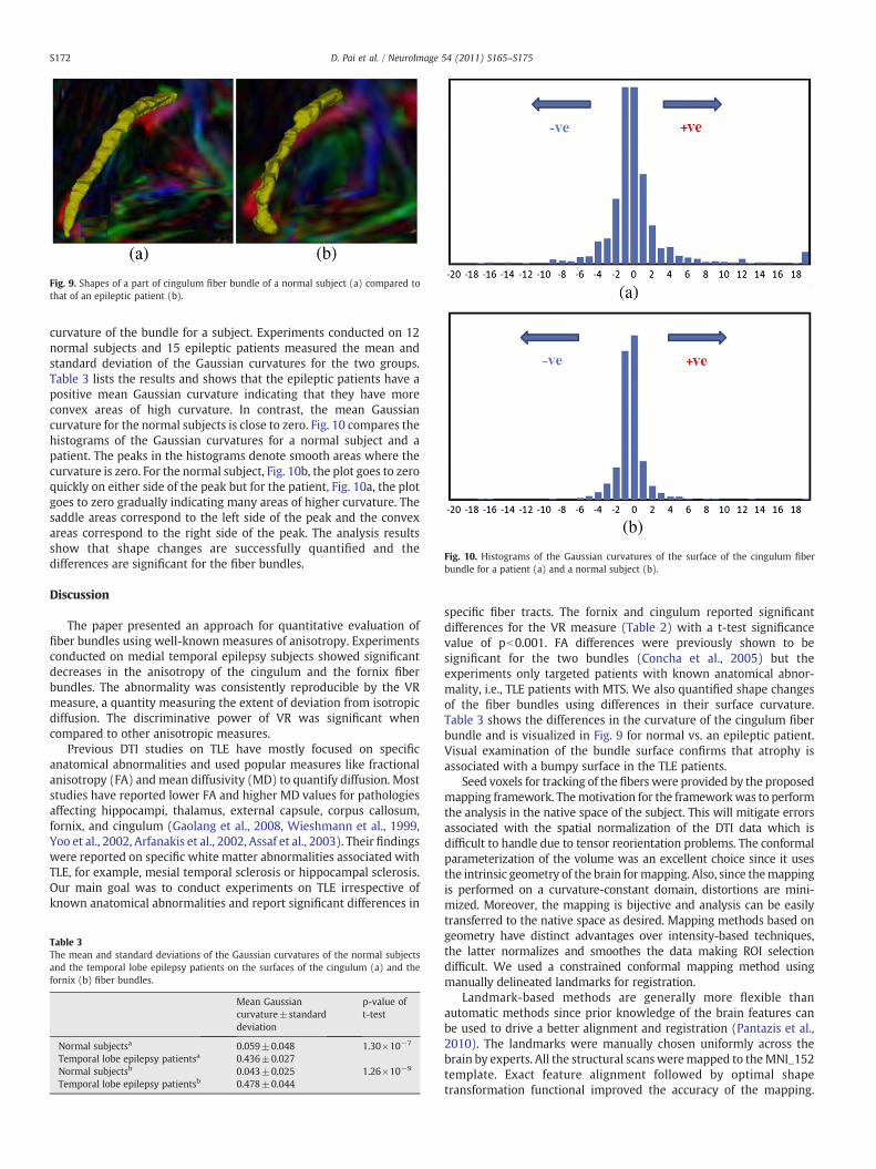
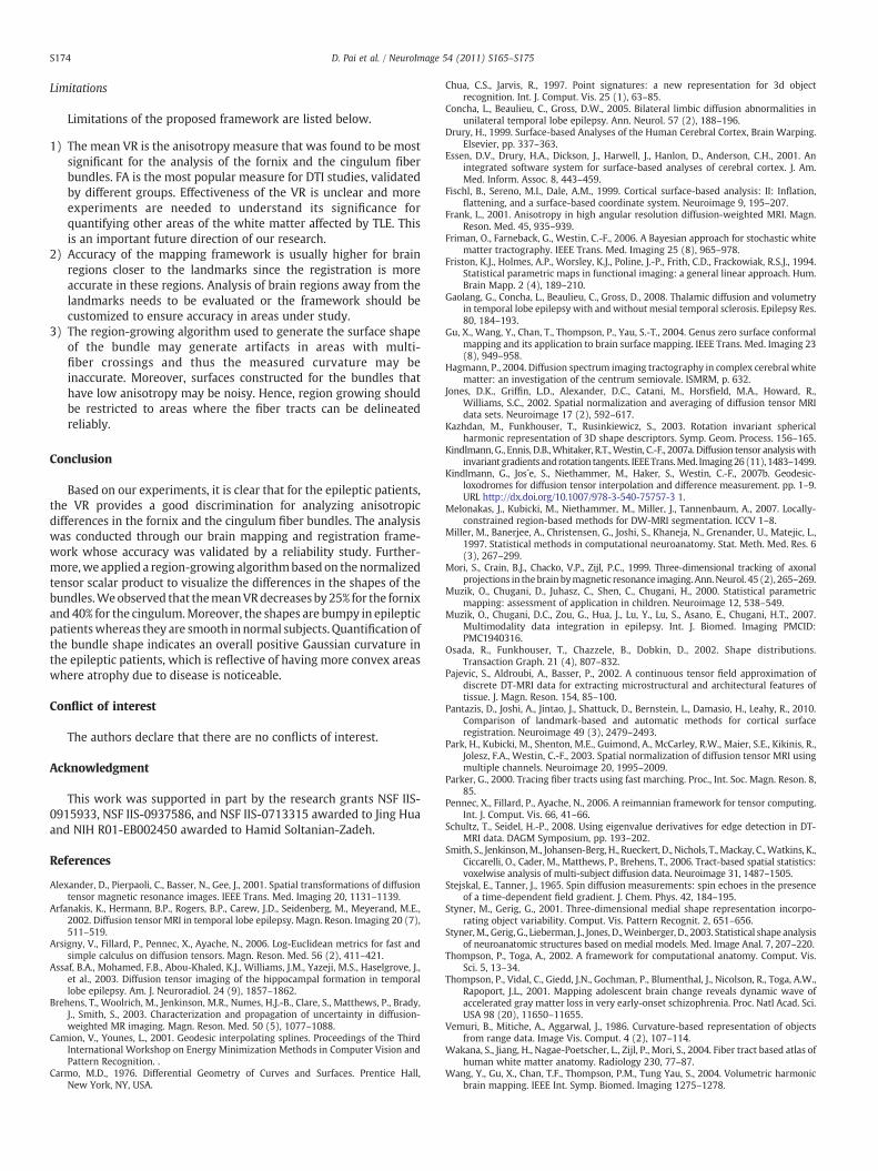
Fig. 9. Shapes of a part of cingulum fiber bundle of a normal subject (a) compared tothat of an epileptic patient (b).

Fig. 10. Histograms of the Gaussian curvatures of the surface of the cingulum fiberbundle for a patient (a) and a normal subject (b).

S172 D. Pai et al. / NeuroImage 54 (2011) S165–S175

curvature of the bundle for a subject. Experiments conducted on 12normal subjects and 15 epileptic patients measured the mean andstandard deviation of the Gaussian curvatures for the two groups.Table 3 lists the results and shows that the epileptic patients have apositive mean Gaussian curvature indicating that they have moreconvex areas of high curvature. In contrast, the mean Gaussiancurvature for the normal subjects is close to zero. Fig. 10 compares thehistograms of the Gaussian curvatures for a normal subject and apatient. The peaks in the histograms denote smooth areas where thecurvature is zero. For the normal subject, Fig. 10b, the plot goes to zeroquickly on either side of the peak but for the patient, Fig. 10a, the plotgoes to zero gradually indicating many areas of higher curvature. Thesaddle areas correspond to the left side of the peak and the convexareas correspond to the right side of the peak. The analysis resultsshow that shape changes are successfully quantified and thedifferences are significant for the fiber bundles.

Discussion

The paper presented an approach for quantitative evaluation offiber bundles using well-known measures of anisotropy. Experimentsconducted on medial temporal epilepsy subjects showed significantdecreases in the anisotropy of the cingulum and the fornix fiberbundles. The abnormality was consistently reproducible by the VRmeasure, a quantity measuring the extent of deviation from isotropicdiffusion. The discriminative power of VR was significant whencompared to other anisotropic measures.

Previous DTI studies on TLE have mostly focused on specificanatomical abnormalities and used popular measures like fractionalanisotropy (FA) andmean diffusivity (MD) to quantify diffusion. Moststudies have reported lower FA and higher MD values for pathologiesaffecting hippocampi, thalamus, external capsule, corpus callosum,fornix, and cingulum (Gaolang et al., 2008, Wieshmann et al., 1999,Yoo et al., 2002, Arfanakis et al., 2002, Assaf et al., 2003). Their findingswere reported on specific white matter abnormalities associated withTLE, for example, mesial temporal sclerosis or hippocampal sclerosis.Our main goal was to conduct experiments on TLE irrespective ofknown anatomical abnormalities and report significant differences in

Table 3The mean and standard deviations of the Gaussian curvatures of the normal subjectsand the temporal lobe epilepsy patients on the surfaces of the cingulum (a) and thefornix (b) fiber bundles.

Mean Gaussiancurvature±standarddeviation

p-value oft-test

Normal subjectsa 0.059±0.048 1.30×10−7

Temporal lobe epilepsy patientsa 0.436±0.027Normal subjectsb 0.043±0.025 1.26×10−9

Temporal lobe epilepsy patientsb 0.478±0.044

specific fiber tracts. The fornix and cingulum reported significantdifferences for the VR measure (Table 2) with a t-test significancevalue of pb0.001. FA differences were previously shown to besignificant for the two bundles (Concha et al., 2005) but theexperiments only targeted patients with known anatomical abnor-mality, i.e., TLE patients with MTS. We also quantified shape changesof the fiber bundles using differences in their surface curvature.Table 3 shows the differences in the curvature of the cingulum fiberbundle and is visualized in Fig. 9 for normal vs. an epileptic patient.Visual examination of the bundle surface confirms that atrophy isassociated with a bumpy surface in the TLE patients.

Seed voxels for tracking of the fibers were provided by the proposedmapping framework. Themotivation for the frameworkwas to performthe analysis in the native space of the subject. This will mitigate errorsassociated with the spatial normalization of the DTI data which isdifficult to handle due to tensor reorientation problems. The conformalparameterization of the volume was an excellent choice since it usesthe intrinsic geometry of the brain formapping. Also, since themappingis performed on a curvature-constant domain, distortions are mini-mized. Moreover, the mapping is bijective and analysis can be easilytransferred to the native space as desired. Mapping methods based ongeometry have distinct advantages over intensity-based techniques,the latter normalizes and smoothes the data making ROI selectiondifficult. We used a constrained conformal mapping method usingmanually delineated landmarks for registration.

Landmark-based methods are generally more flexible thanautomatic methods since prior knowledge of the brain features canbe used to drive a better alignment and registration (Pantazis et al.,2010). The landmarks were manually chosen uniformly across thebrain by experts. All the structural scansweremapped to theMNI_152template. Exact feature alignment followed by optimal shapetransformation functional improved the accuracy of the mapping.

S173D. Pai et al. / NeuroImage 54 (2011) S165–S175

An affine registration between the MRI and the corresponding DTIcompleted the mapping from the MNI_152 template to each in-dividual DTI image.

Bias in DTI analysis is attributed to artifacts due to subject motionor distortion effects during acquisition and operator dependence. Thedatasets were corrected for Eddy current effects using the toolsavailable in FSL. The images were inspected after the correction andcompared to the corresponding T1 image for geometrical distortion inbrain regions where the ROIs would be defined. Onlymatched DTI andT1 scans were included in the study.

The operator can bias the ROI selection process and hence wefollowed a strict set of protocols for ROI selection as described in aprevious section. Three raters placed the ROIs on 5 datasets toevaluate the inter-rater and intra-rater reliability which turned out tobe excellent (Table 1). Moreover, ROIs defined on the MRI templateand transformed to the DTI using the mapping parameters and theaffine registration parameters showed good reproducibility of thefibers (inter-modal reliability).

Probabilistic tracking of fibers was the preferred choice because ofits inherent ability to account for uncertainty in the tracking. To getreasonable connectivity information from the tracking, a largenumber of samples are generated. The generated paths representthe sampling space of the seed voxel. From the sampling space, onlyfiber paths that pass through these ROIs were chosen for theanisotropy analysis. Connection probabilities were not taken intoconsideration in this paper. Since the probabilities depend on the seedlocations of the ROIs, it is unclear if changes in connectivity aresignificant at this time.

Finally, the surface of the fiber bundle was generated using theentire diffusion tensor information at each voxel. A simple region-

Fig. 11. (a) Curvature histogram when no noise is added. (b)–(d) Curvature histograms whshow some curvature values away from zero but the overall distribution is maintained.

growing algorithm was employed to extract the surface from thebundle volume. We used the normalized tensor scalar product as ameasure of the tensor. The normalization of the tensor makes itindependent of the size of the tensor and the region-growingalgorithm only depends on the shape and the orientation.

To check for artifacts in the region-growing output, a sensitivityanalysis was performed. We simulated fiber bundle degradation witha Gaussian disturbing function on a normal dataset. The curvaturewith no degradation was 0.01 which gradually increased to 0.11 for10% degradation, 0.19 for 20% degradation, and 0.27 for 30%degradation. The sensitivity analysis confirmed that the method wassensitive to changes in the fiber bundles and thus was an excellentmethod to analyze the shape.

We also simulated white matter degradation by adding Gaussianwhite noise, N(0;σ), where σ is the standard deviation. A normaldataset was subjected to varying levels of noise controlled by thevariance σ2 of the noise. The region-growing algorithm was executedand the fiber bundle surfaces were extracted for three noisy datasetsat three different noise levels, σ2=10, σ2=20, and σ2=30. ThemeanGaussian curvatures for noise levels σ2=10, σ2=20, and σ2=30were calculated as 0.02, 0.03, and 0.05 respectively. The distributionsof the Gaussian curvature are illustrated in Fig. 11. As noise levelsincrease, more convex and saddle surfaces appear as is evident fromthe histogram. However, the overall distribution is consistent and themean curvature is not influenced by noise. Region growing doesindeed have its disadvantages. The results of the algorithm is noisy inplaces where fiber mixing and fiber crossing is rampant and hence isnot reliable for calculating curvature. In other words, only a well-delineated fiber tract will subsequently generate a good bundlesurface for measuring curvature.

en noise is simulated with σ2=10, σ2=20, and σ2=30, respectively. The histograms

S174 D. Pai et al. / NeuroImage 54 (2011) S165–S175

Limitations

Limitations of the proposed framework are listed below.

1) The mean VR is the anisotropy measure that was found to be mostsignificant for the analysis of the fornix and the cingulum fiberbundles. FA is the most popular measure for DTI studies, validatedby different groups. Effectiveness of the VR is unclear and moreexperiments are needed to understand its significance forquantifying other areas of the white matter affected by TLE. Thisis an important future direction of our research.

2) Accuracy of the mapping framework is usually higher for brainregions closer to the landmarks since the registration is moreaccurate in these regions. Analysis of brain regions away from thelandmarks needs to be evaluated or the framework should becustomized to ensure accuracy in areas under study.

3) The region-growing algorithm used to generate the surface shapeof the bundle may generate artifacts in areas with multi-fiber crossings and thus the measured curvature may beinaccurate. Moreover, surfaces constructed for the bundles thathave low anisotropy may be noisy. Hence, region growing shouldbe restricted to areas where the fiber tracts can be delineatedreliably.

Conclusion

Based on our experiments, it is clear that for the epileptic patients,the VR provides a good discrimination for analyzing anisotropicdifferences in the fornix and the cingulum fiber bundles. The analysiswas conducted through our brain mapping and registration frame-work whose accuracy was validated by a reliability study. Further-more,we applied a region-growing algorithmbased on thenormalizedtensor scalar product to visualize the differences in the shapes of thebundles.Weobserved that themeanVRdecreases by 25% for the fornixand 40% for the cingulum.Moreover, the shapes are bumpy in epilepticpatientswhereas they are smooth in normal subjects. Quantification ofthe bundle shape indicates an overall positive Gaussian curvature inthe epileptic patients, which is reflective of having more convex areaswhere atrophy due to disease is noticeable.

Conflict of interest

The authors declare that there are no conflicts of interest.

Acknowledgment

This work was supported in part by the research grants NSF IIS-0915933, NSF IIS-0937586, and NSF IIS-0713315 awarded to Jing Huaand NIH R01-EB002450 awarded to Hamid Soltanian-Zadeh.

References

Alexander, D., Pierpaoli, C., Basser, N., Gee, J., 2001. Spatial transformations of diffusiontensor magnetic resonance images. IEEE Trans. Med. Imaging 20, 1131–1139.

Arfanakis, K., Hermann, B.P., Rogers, B.P., Carew, J.D., Seidenberg, M., Meyerand, M.E.,2002. Diffusion tensor MRI in temporal lobe epilepsy. Magn. Reson. Imaging 20 (7),511–519.

Arsigny, V., Fillard, P., Pennec, X., Ayache, N., 2006. Log-Euclidean metrics for fast andsimple calculus on diffusion tensors. Magn. Reson. Med. 56 (2), 411–421.

Assaf, B.A., Mohamed, F.B., Abou-Khaled, K.J., Williams, J.M., Yazeji, M.S., Haselgrove, J.,et al., 2003. Diffusion tensor imaging of the hippocampal formation in temporallobe epilepsy. Am. J. Neuroradiol. 24 (9), 1857–1862.

Brehens, T., Woolrich, M., Jenkinson, M.R., Numes, H.J.-B., Clare, S., Matthews, P., Brady,J., Smith, S., 2003. Characterization and propagation of uncertainty in diffusion-weighted MR imaging. Magn. Reson. Med. 50 (5), 1077–1088.

Camion, V., Younes, L., 2001. Geodesic interpolating splines. Proceedings of the ThirdInternational Workshop on Energy Minimization Methods in Computer Vision andPattern Recognition. .

Carmo, M.D., 1976. Differential Geometry of Curves and Surfaces. Prentice Hall,New York, NY, USA.

Chua, C.S., Jarvis, R., 1997. Point signatures: a new representation for 3d objectrecognition. Int. J. Comput. Vis. 25 (1), 63–85.

Concha, L., Beaulieu, C., Gross, D.W., 2005. Bilateral limbic diffusion abnormalities inunilateral temporal lobe epilepsy. Ann. Neurol. 57 (2), 188–196.

Drury, H., 1999. Surface-based Analyses of the Human Cerebral Cortex, Brain Warping.Elsevier, pp. 337–363.

Essen, D.V., Drury, H.A., Dickson, J., Harwell, J., Hanlon, D., Anderson, C.H., 2001. Anintegrated software system for surface-based analyses of cerebral cortex. J. Am.Med. Inform. Assoc. 8, 443–459.

Fischl, B., Sereno, M.I., Dale, A.M., 1999. Cortical surface-based analysis: II: Inflation,flattening, and a surface-based coordinate system. Neuroimage 9, 195–207.

Frank, L., 2001. Anisotropy in high angular resolution diffusion-weighted MRI. Magn.Reson. Med. 45, 935–939.

Friman, O., Farneback, G., Westin, C.-F., 2006. A Bayesian approach for stochastic whitematter tractography. IEEE Trans. Med. Imaging 25 (8), 965–978.

Friston, K.J., Holmes, A.P., Worsley, K.J., Poline, J.-P., Frith, C.D., Frackowiak, R.S.J., 1994.Statistical parametric maps in functional imaging: a general linear approach. Hum.Brain Mapp. 2 (4), 189–210.

Gaolang, G., Concha, L., Beaulieu, C., Gross, D., 2008. Thalamic diffusion and volumetryin temporal lobe epilepsy with and without mesial temporal sclerosis. Epilepsy Res.80, 184–193.

Gu, X., Wang, Y., Chan, T., Thompson, P., Yau, S.-T., 2004. Genus zero surface conformalmapping and its application to brain surface mapping. IEEE Trans. Med. Imaging 23(8), 949–958.

Hagmann, P., 2004. Diffusion spectrum imaging tractography in complex cerebral whitematter: an investigation of the centrum semiovale. ISMRM, p. 632.

Jones, D.K., Griffin, L.D., Alexander, D.C., Catani, M., Horsfield, M.A., Howard, R.,Williams, S.C., 2002. Spatial normalization and averaging of diffusion tensor MRIdata sets. Neuroimage 17 (2), 592–617.

Kazhdan, M., Funkhouser, T., Rusinkiewicz, S., 2003. Rotation invariant sphericalharmonic representation of 3D shape descriptors. Symp. Geom. Process. 156–165.

Kindlmann, G., Ennis, D.B.,Whitaker, R.T.,Westin, C.-F., 2007a. Diffusion tensor analysiswithinvariant gradients androtation tangents. IEEETrans.Med. Imaging26 (11), 1483–1499.

Kindlmann, G., Jos´e, S., Niethammer, M., Haker, S., Westin, C.-F., 2007b. Geodesic-loxodromes for diffusion tensor interpolation and difference measurement. pp. 1–9.URL http://dx.doi.org/10.1007/978-3-540-75757-3 1.

Melonakas, J., Kubicki, M., Niethammer, M., Miller, J., Tannenbaum, A., 2007. Locally-constrained region-based methods for DW-MRI segmentation. ICCV 1–8.

Miller, M., Banerjee, A., Christensen, G., Joshi, S., Khaneja, N., Grenander, U., Matejic, L.,1997. Statistical methods in computational neuroanatomy. Stat. Meth. Med. Res. 6(3), 267–299.

Mori, S., Crain, B.J., Chacko, V.P., Zijl, P.C., 1999. Three-dimensional tracking of axonalprojections in the brain bymagnetic resonance imaging. Ann.Neurol. 45 (2), 265–269.

Muzik, O., Chugani, D., Juhasz, C., Shen, C., Chugani, H., 2000. Statistical parametricmapping: assessment of application in children. Neuroimage 12, 538–549.

Muzik, O., Chugani, D.C., Zou, G., Hua, J., Lu, Y., Lu, S., Asano, E., Chugani, H.T., 2007.Multimodality data integration in epilepsy. Int. J. Biomed. Imaging PMCID:PMC1940316.

Osada, R., Funkhouser, T., Chazzele, B., Dobkin, D., 2002. Shape distributions.Transaction Graph. 21 (4), 807–832.

Pajevic, S., Aldroubi, A., Basser, P., 2002. A continuous tensor field approximation ofdiscrete DT-MRI data for extracting microstructural and architectural features oftissue. J. Magn. Reson. 154, 85–100.

Pantazis, D., Joshi, A., Jintao, J., Shattuck, D., Bernstein, L., Damasio, H., Leahy, R., 2010.Comparison of landmark-based and automatic methods for cortical surfaceregistration. Neuroimage 49 (3), 2479–2493.

Park, H., Kubicki, M., Shenton, M.E., Guimond, A., McCarley, R.W., Maier, S.E., Kikinis, R.,Jolesz, F.A., Westin, C.-F., 2003. Spatial normalization of diffusion tensor MRI usingmultiple channels. Neuroimage 20, 1995–2009.

Parker, G., 2000. Tracing fiber tracts using fast marching. Proc., Int. Soc. Magn. Reson. 8,85.

Pennec, X., Fillard, P., Ayache, N., 2006. A reimannian framework for tensor computing.Int. J. Comput. Vis. 66, 41–66.

Schultz, T., Seidel, H.-P., 2008. Using eigenvalue derivatives for edge detection in DT-MRI data. DAGM Symposium, pp. 193–202.

Smith, S., Jenkinson,M., Johansen-Berg,H., Rueckert, D., Nichols, T.,Mackay, C.,Watkins, K.,Ciccarelli, O., Cader, M., Matthews, P., Brehens, T., 2006. Tract-based spatial statistics:voxelwise analysis of multi-subject diffusion data. Neuroimage 31, 1487–1505.

Stejskal, E., Tanner, J., 1965. Spin diffusion measurements: spin echoes in the presenceof a time-dependent field gradient. J. Chem. Phys. 42, 184–195.

Styner, M., Gerig, G., 2001. Three-dimensional medial shape representation incorpo-rating object variability. Comput. Vis. Pattern Recognit. 2, 651–656.

Styner,M., Gerig,G., Lieberman, J., Jones, D.,Weinberger, D., 2003. Statistical shape analysisof neuroanatomic structures based on medial models. Med. Image Anal. 7, 207–220.

Thompson, P., Toga, A., 2002. A framework for computational anatomy. Comput. Vis.Sci. 5, 13–34.

Thompson, P., Vidal, C., Giedd, J.N., Gochman, P., Blumenthal, J., Nicolson, R., Toga, A.W.,Rapoport, J.L., 2001. Mapping adolescent brain change reveals dynamic wave ofaccelerated gray matter loss in very early-onset schizophrenia. Proc. Natl Acad. Sci.USA 98 (20), 11650–11655.

Vemuri, B., Mitiche, A., Aggarwal, J., 1986. Curvature-based representation of objectsfrom range data. Image Vis. Comput. 4 (2), 107–114.

Wakana, S., Jiang, H., Nagae-Poetscher, L., Zijl, P., Mori, S., 2004. Fiber tract based atlas ofhuman white matter anatomy. Radiology 230, 77–87.

Wang, Y., Gu, X., Chan, T.F., Thompson, P.M., Tung Yau, S., 2004. Volumetric harmonicbrain mapping. IEEE Int. Symp. Biomed. Imaging 1275–1278.

S175D. Pai et al. / NeuroImage 54 (2011) S165–S175

Wang, Y., Lui, L., Chan, T., Thompson, P., 2005. Optimization of brain conformal mappingwith landmarks. Proc. MICCAI, pp. 675–683.

Wieshmann, U.C., Clark, C.A., Symms, M.R., Barker, G.J., Birnie, K.D., Shorvon, S.D., 1999.Water diffusion in the human hippocampus in epilepsy. Magn. Reson. Imaging 17,29–36.

Woods, R.P., Grafton, S.T., Holmes, C.J., Cherry, S.R., Mazziotta, J.C., 1998. Automatedimage registration: I. General methods and intrasubject, intramodality validation.J. Comput. Assist. Tomogr. 22, 139–152.

Yoo, S.Y., Chang, K.H., Song, I.C., Han, M.H., Kwon, B.J., Lee, S.H., et al., 2002. Apparentdiffusion coefficient value of the hippocampus in patients with hippocampalsclerosis and in healthy volunteers. Am. J. Neuroradiol. 23 (5), 809–812.

Zhang, D., 1999. Harmonic Shape Images: a 3D Free-form Surface Representation andits Applications in Surface Matching. Ph.D. Dissertation, Robotics Institute, CarnegieMellon University.

Zou, G., Hua, J., Gu, X., 2006. An approach for intersubject analysis of 3D brain imagesbased on conformal geometry. Proceedings, ICIP, pp. 1193–1196.