Evaluation of Chemical Equilibrium and Non-Equilibrium ... · br/CFD/projetos/cfd5/relatorio_tecnico_1. CHEMICAL EQUILIBRIUM ... (1987) 10 6 8 H 2 O, O 2, H 2, OH, O, H, HO 2, H 2

J. Aerosp. Technol. Manag., São José dos Campos, Vol.7, No 1, pp.31-42, Jan.-Mar., 2015

ABSTRACT: Nine chemical reaction models for equilibrium schemes and six chemical models for non-equilibrium ones are studied, considering different conditions found in real liquid oxygen/liquid hydrogen rocket engines. Comparisons between two eight-species models have shown that the most complex is the best one. Besides, it was also verified that the most complex model has been the fastest, among six- and eight-species models. Both combustion temperature and thermochemical/transport properties depend only on the chemical species considered by the used model. Comparisons among results from the implemented code (Gibbs 1.3), Chemical Equilibrium with Applications and Thermochemical Information and Equilibrium Calculations, these last two codes from NASA, have shown that Gibbs 1.3 evaluates correctly both combustion temperature and thermochemical properties. Furthermore, analyses have shown that mass generation rates are very dependent on third body reaction equations and forward reaction constants.

KEYWORDS: Chemical reaction models, Chemical equilibrium, Combustion temperature, Non-equilibrium.

Evaluation of Chemical Equilibrium and Non-Equilibrium Properties for LOX/LH2 Reaction SchemesCarlos Henrique Marchi1, Luciano Kiyoshi Araki1

INTRODUCTION

The hydrogen/oxygen (H2/O2) combustion systems have many attractive features, including high specific impulse for rocket engine applications, clean-burning feature for achieving environmentally friendly combustion products, reliable ignition and high combustion efficiency. Even though there are only two elements involved, the chemical reaction mechanisms of H2/O2 systems are quite complex, involving various steps of chain reactions. This system is also important as a subsystem in the oxidation process of hydrocarbons and moist carbon monoxide (Kuo, 2005; Turns, 2000).

Due to the fact that complex mechanisms are evolutionary products of the chemists’ thoughts and experiments (Turns, 2000), several studies have been published recently about the mathematical models for hydrogen ignition, the reaction kinetics and/or the flame propagation. For example, Bedarev and Fedorov (2006) compared three mathematical models of hydrogen ignition, for the reactive flow behind the front of an initiating shock wave. Smith et al. (2007) studied the combustion zone near the injection of a liquid rocket engine thrust chamber in order to evaluate the influence of reduced pressure on the flame formation and combustion efficiency. Fernández-Galisteo et al. (2009) proposed and studied a short mechanism consisting of seven elementary reactions for hydrogen-air lean-flame burning velocities.

The knowledge of species formed by liquid oxygen/liquid hydrogen (LOX/LH2) combustion is the first step for a complete study involving combustion mixture gases flow, heat transfer and coolant pressure drop in a real cryogenic H2O2 rocket engine, such as Space Shuttle or Vulcain Engine of Ariane Launcher.

doi: 10.5028/jatm.v7i1.426

1.Universidade Federal do Paraná – Curitiba/PR – Brazil.

Author for correspondence: Luciano Kiyoshi Araki | Universidade Federal do Paraná | Departamento de Engenharia Mecânica | Caixa Postal 19040 | CEP: 81.531-980 Curitiba/PR – Brazil | Email: [email protected]

Received: 10/10/2014 | Accepted: 01/08/2015


32Marchi, C.H. and Araki, L.K.

At high temperatures, such as those found in rocket thrust chambers, effects of dissociation become important and new species must be considered (Anderson Jr., 2003). In such situations, it is necessary the study of chemical equilibrium and non-chemical equilibrium.

For both equilibrium and non-equilibrium reaction schemes, thermodynamic properties of species are required to define properly the mixture of gases’ composition. Such properties can be easily taken from thermodynamic tables and/or graphics. In this work, however, it is used the method presented by McBride et al. (1993), in which libraries for thermodynamic and transport properties for pure species can be found. Nine different reaction models are used to obtain equilibrium composition. In the simplest one, only 3 chemical species are considered: H2, O2 and H2O, without chemical dissociation reactions. In the most complete scheme, 8 species (H2, O2, H2O, H, O, OH, H2O2 and HO2) and 18 chemical reactions are studied. For non-equilibrium studies, 6 different models are used, involving only 6 or 8 species. These models are essentially the same ones used at equilibrium schemes, but taking into account third body species (and also, third body reactions).

Two different kinds of comparisons are presented in this work. Firstly, five couples of temperature and pressure values are chosen, intending to cover all range of values found in a real rocket thrust chamber. The results were compared with those obtained from Chemical Equilibrium with Applications (CEA; Glenn Research Center, 2005) and Thermochemical Information and Equilibrium Calculations (Teqworks; Gordon and McBride, 1971), both codes from NASA. Secondly, it is studied the combustion temperature of LOX/LH2 reactions at different oxidant/fuel mass ratios and combustion pressures. The obtained results were compared with CEA and Teqworks codes and, for some cases, with other results from literature. Furthermore, results for species generation rates for non-equilibrium models are presented.

The importance of this study is to compare both equilibrium and non-equilibrium models, specially in relation to the importance of the chemical intermediate reactions, which are the base of non-equilibrium flows. The numerical code, whose results are presented in this study, is available from: ftp://ftp.demec.ufpr.br/CFD/projetos/cfd5/relatorio_tecnico_1.

CHEMICAL EQUILIBRIUM

The applied methodology in this work to obtain chemical equilibrium parameters of a mixture of gases can be found in

Kuo (2005) and is briefly explained in this section. Firstly, it is considered a chemical reaction in the form:

where A represents each chemical species’ symbol, i corresponds to the number of each chemical species, N is the total number of chemical species, j corresponds to a specific chemical reaction, L is the total number of chemical reactions,

ѵ’

ij and ѵ’’ij are, in this order, the stoichiometric coefficients of

chemical species i in reaction j existent in reagents and products and kf and kb represent, respectively, forward and backward reaction constants.

At chemical equilibrium conditions, for each single chemical reaction j, there is a specific equilibrium constant (Kj), based on partial pressures (pi). This constant shows how the forward and the backward ways of a reaction j are related at a specific temperature and can be calculated by:

The Kj can also be obtained from the variation of the Gibbs 1.3 free energy (ΔGj), which can be evaluated by:

where gi corresponds to the Gibbs 1.3 free energy of species i, that can be calculated with the methodology presented by McBride et al. (1993), in which values of constant-pressure specific heat (c), enthalpy (h) and Gibbs 1.3 free energy (g) can be estimated by polynomial equations:

where coefficients for thermodynamic properties estimative (ak) have particular values for every single chemical species i,

(1)

(2)

(3)

(4)

(5)

(6)


33Evaluation of Chemical Equilibrium and Non-Equilibrium Properties for LOX/LH2 Reaction Schemes

Ru is the universal constant for perfect gases (8.314510 J/molK) and T corresponds to the absolute temperature (in K) at which the property is been evaluated.

Therefore, Kj can also be determinated by:

they differ from one dissociation equation at least, reason for considering them independent models.

Model 0Model 0 is the simplest model implemented at Gibbs 1.3.

Dissociation effects are not taken into account by this model, presenting the worst results at high temperatures. The importance of this model, however, is on its equations, that will be used in other models for further calculations. Its global reaction equation is given by:

Similarly, it is possible to evaluate transport properties, such as viscosity (μ) and heat conductivity (k) for a single species i, using the following relations, adapted from McBride et al. (1993) to SI units:

and

where bk e dk (k = 1 to 4) are the particular coefficients for each chemical species i.

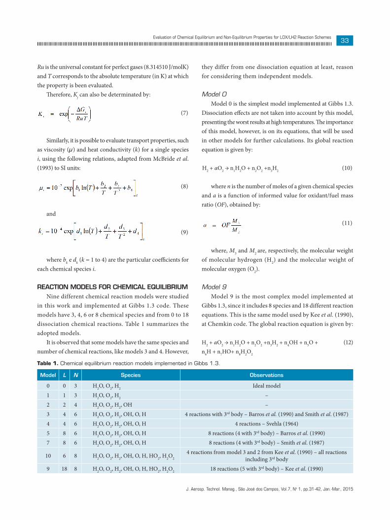
REACTION MODELS FOR CHEMICAL EQUILIBRIUMNine different chemical reaction models were studied

in this work and implemented at Gibbs 1.3 code. These models have 3, 4, 6 or 8 chemical species and from 0 to 18 dissociation chemical reactions. Table 1 summarizes the adopted models.

It is observed that some models have the same species and number of chemical reactions, like models 3 and 4. However,

Model L N Species Observations

0 0 3 H2O, O2, H2 Ideal model1 1 3 H2O, O2, H2 –2 2 4 H2O, O2, H2, OH –3 4 6 H2O, O2, H2, OH, O, H 4 reactions with 3rd body – Barros et al. (1990) and Smith et al. (1987)4 4 6 H2O, O2, H2, OH, O, H 4 reactions – Svehla (1964)5 8 6 H2O, O2, H2, OH, O, H 8 reactions (4 with 3rd body) – Barros et al. (1990)7 8 6 H2O, O2, H2, OH, O, H 8 reactions (4 with 3rd body) – Smith et al. (1987)

10 6 8 H2O, O2, H2, OH, O, H, HO2, H2O24 reactions from model 3 and 2 from Kee et al. (1990) – all reactions

including 3rd body9 18 8 H2O, O2, H2, OH, O, H, HO2, H2O2 18 reactions (5 with 3rd body) – Kee et al. (1990)

Table 1. Chemical equilibrium reaction models implemented in Gibbs 1.3.

where n is the number of moles of a given chemical species and a is a function of informed value for oxidant/fuel mass ratio (OF), obtained by:

where, M3 and M2 are, respectively, the molecular weight of molecular hydrogen (H2) and the molecular weight of molecular oxygen (O2).

Model 9Model 9 is the most complex model implemented at

Gibbs 1.3, since it includes 8 species and 18 different reaction equations. This is the same model used by Kee et al. (1990), at Chemkin code. The global reaction equation is given by:

(7)

(10)

(11)

(8)

(9)

(12)H2 + αO2 → n1H2O + n2O2 +n3H2 + n4OH + n5O + n6H + n7HO+ n8H2O2

H2 + αO2 → n1H2O + n2O2 +n3H2



Table 2 presents the dissociation equations related to model 9.The resulting system of equations, which must be solved

in order to obtain the composition at chemical equilibrium, is presented in Table 3 (where p is the total pressure).

ALGORITHM FOR CHEMICAL EQUILIBRIUM This section presents the Gibbs 1.3 chemical equilibrium

algorithm. It consists in ten steps: • Definition of data: reactive model number, T, p, OF

and numeric parameters (number of iterations and tolerances).

• Reading of thermodynamic coefficients (aki) for constant-pressure specific heat, enthalpy and Gibbs 1.3 free energy (Eq. 4 to 6).

• Coefficients’ evaluation of Eq. (10): a is based on Eq. (11) and n1, n2 and n3 are obtained from a simple chemical equilibrium calculus.

• Initialization of reaction degrees (εj) for all dissociation reactions, with null-value.

• Evaluation of initial number of moles for every single reactive model species (ni) and total number of moles (n), based on variables from items Coefficients’ evaluation and Initialization of reaction degrees.

• Evaluation of gi, Gibbs 1.3 free energy change and equilibrium constant based on partial pressure for reaction j by Eq. (7).

• Iterative evaluation, for the first dissociation reaction (ε1), by Newton-Raphson method (Turns, 2000), with calculations made until the maximum number of iterations or up to the tolerance is achieved. This is made for the second dissociation reaction and so on, until the last reaction (L).

• Actualization of the number of moles for ni and n, with obtained results for εj calculated in item “Iterative evaluation”.

• Evaluation of total number of moles variation (Δn). Return to item “Iterative evaluation” until the maximum number of iterations is achieved or while Δn is greater than the chosen tolerance.

• Evaluation of mixture properties, such as mean molecular weight, molar and mass fractions, gas mixture density, constant-pressure specific heat, ratio of specific heats, gases mixture constant, viscosity and thermal conductivity.

COMBUSTION TEMPERATURE

Combustion temperature determination (also known as adiabatic flame temperature) is basically the same problem of

1 K1pn4n6 = n1n2 K2n3n = n6

1p3 K3n2n = n5

2p4 K4pn2n6 = n7n5 K5n8n = n4

2p6 K6n2n3 = n4

2

7 K7n3n4 = n1n6

8 K8n2n6 = n4n5

9 K9n3n5 = n4 n6

10 K10pn2n6 = n7n11 K11n4n7 = n1n2

12 K12n6n7 = n42

13 K13n5n7 = n2n4

14 K14n42 = n1n5

15 K15n6n7 = n2 n3

16 K16n72 = n2n8

17 K17n6n8 = n3n7

18 K18n4n8 = n1 n7

Table 3. Non-linear equations system of model 9.

1 H + OH + D3 ←→ H2O + D3

2 H2 + D3 ←→ 2H +D3

3 O2 + D3 ←→ 2O + D3

4 H + O2 + D3 ←→ HO2 + D3

5 H2O2 + D3 ←→ 2OH + D3

6 H2 + O2 ←→ 2OH7 OH + H2 ←→ H2O + H8 H + O2 ←→ OH + O9 O + H2 ←→ OH + H

10 H + 2O2 ←→ HO2 + O2

11 OH + HO2 ←→ H2O + O2

12 H + HO2 ←→ 2OH13 O + HO2 ←→ O2 + OH14 2OH ←→ O + H 2O15 H + HO2 ←→ H2 + O2

16 2HO2 ←→ H2O2 + O2

17 H2O2 + H ←→ HO2 + H2

18 H2O2 + OH ←→ H2O + HO2

Table 2. Chemical reactions taken into account by model 9.

D3: 3rd body.



chemical equilibrium; however, in this case, only the temperatures (or enthalpies) of reagents are known, as well as the chamber pressure and the OF. The problem is basically to equalize the enthalpy of reagents with the enthalpy of products. However, as the composition of gas mixture is dependent on the temperature, an iterative method for obtaining the combustion temperature is needed. In this work, it was used a methodology based on bisection method (Chapra and Canale, 1994), with chemical equilibrium parameters calculated by equations presented by Kuo (2005). The same chemical reaction models presented in Table 1 are valid for the implemented combustion temperature determination code.

Table 3 presents the non-linear equation system of model 9.

ALGORITHM FOR ADIABATIC COMBUSTIONThe implemented algorithm for adiabatic combustion

temperature’s determination is presented in this section. It consists of the following steps:

• Definition of data: reactive model number, temperature or enthalpy of reagents, p, OF and numeric parameters (iteration numbers and tolerances).

• Idem steps “Reading of thermodynamic coefficients” to “Evaluation of initial number of moles for every single reactive model species and total number of moles” of the section “Algorithm for chemical equilibrium”.

• Evaluation of total enthalpy of reagents by:

• Evaluation of temperature variation (ΔT) between old and new temperature. Return to item “Idem steps ‘Reading of thermodynamic coefficients’ to ‘Evaluation of initial number of moles for every single reactive model species and total number of moles’ of the section ‘Algorithm for chemical equilibrium’” until the maximum number of iterations is achieved or while ΔT is greater than the chosen tolerance.

• Evaluation of mixture’s properties, such as mean molecular weight, molar and mass fractions, gas mixture’s density, constant-pressure specific heat, ratio of specific heats and gases mixture’s constant.

CHEMICAL NON-EQUILIBRIUM

Chemical and vibrational processes take place because of molecular collisions and/or radiation. Third body species have an important role on these processes, providing the energy required to other species by collisions, in order to allow chemical reactions occur. These interactions, however, demand a period of time, something that may not come true in some practical situations, such as the gas flow in a rocket nozzle engine. In such cases, equilibrium conditions are not reached, once it demands infinitely large reaction rates, i.e. instantaneous adjustments to the local temperature and pressure of gases. Therefore, regions where non-equilibrium phenomena take place will appear through the flow and, for these cases, an alternative methodology must be used, in order to consider the reaction time over the composition of the gas mixture (Anderson Jr., 2003).

To evaluate the mass generation rate of chemical species, some variables must be presented and defined. The first one is the progression rate of reaction j (γj), which is concerned about the difference between forward and backward reaction rates and is given by:

where hfuel and hoxidant indicate, respectively, the fuel enthalpy (in the studied case, hydrogen) and the oxidant enthalpy (oxygen).

• First guess: the combustion temperature is considered to be 3,150 K (mean value between 300 and 6,000 K, which corresponds to the range of applicability for aki).

• Idem steps “Evaluation of Gibbs 1.3 free energy for each single species” to “Evaluation of total number of moles variation” of the section “Algorithm for chemical equilibrium”.

• Evaluation of total enthalpy of products by Eq. (14):

• New estimative for the combustion temperature with bisection method (Chapra and Canale, 1994).

where Ci is the molar concentration of species i in mixture. The species generation rate (θj) is obtained from the product between Eq. (15) and the third body effective concentration and can be estimated by:

HR = hfuel + ahoxidant (13)

(14)

(15)

(16)Ѳj = λj . γj



where λj is defined as:

in which αij is the efficiency of chemical species i at a dissociation reaction j.

Unfortunately, there is a lack of information about the effi-ciency of the existent molecules in a dissociation reaction model. Consequently, it is commonly adopted that the efficiencies of all chemical species are equal to unit and, in this case, the concen-tration of third body species corresponds to the whole number of existent species (Barros et al., 1990).

The determination of mass generation rates is obtained by the product of Eq. (16) and molecular weight (Mi) of the species, resulting in:

where Δѵij is calculated by Δѵij = ѵ’’ij - ѵ’ij and represents the

difference between formed and consumed number of moles for a reaction j.

REACTION MODELS FOR NON-EQUILIBRIUMSix different non-equilibrium reaction models are studied

in this work and implemented at code Gibbs 1.3. These models have 6 or 8 chemical species, corresponding to models 3, 5, 7, 9 and 10 from equilibrium schemes, according to Table 1. It is noted that model 3 was split into two non-equilibrium models. Despite the fact that each model has the same species, two different equation systems for forward reaction constants (kf) were considered from works of Barros et al. (1990) and Smith et al. (1987), which justifies to treat them as two independent models in this section.

MODEL 3.1Model 3 from equilibrium schemes was split into two

different models in non-equilibrium schemes, named model 3.1 and model 3.2. Both models include six different species and the chemical reactions presented in Table 4.

However, for each chemical reaction of model 3.1, one should take into account the forward reaction constants from Barros et al. (1990), which are obtained by the relations presented in Table 5.

1 H + OH + D3 ←→ H2O + D3

2 2H + D3 ←→ H2 + D3

3 2O + D3 ←→ O2 + D3

4 O + H + D3 ←→ OH + D3

1 kf1 = 3.626 x 1019/T2 kf2 = 7.5 x 1017/T3 kf3 = 3.626 x 1018/T4 kf4 = 3.626 x 1018/T

1 [H2O]: ώ1 = M1 . θ1

2 [O2]: ώ2 = M2 . θ3

3 [H2]: ώ3 = M3 . θ2

4 [OH]: ώ4 = M4 . (θ4 - θ1)

5 [O]: ώ5 = -M5 . (2θ3 + θ4)

6 [H]: ώ6 = -M6 . (θ1 + 2θ2 + θ4)

Table 4. Chemical reactions by models 3.1 and 3.2.

Table 5. Forward reaction constants by model 3.1.

Table 6. Mass generation rates of model 3.1.

D3: 3rd body.

Based on the forward reaction constants, the progression rates for all reactions can be evaluated by Eq. (15). Taking the efficiencies of all species equal to unity, the parameter λ corresponds to the total concentration (C), and the reaction parameters (θj) can be evaluated as θj = C x γj, according to Eq. (16). The ώj can be evaluated by the equations presented in Table 6.

ALGORITHM FOR NON-EQUILIBRIUMThe implemented algorithm for non-equilibrium is pre-

sented in this section. It consists of the eight following steps:• Definition of data: reactive model number, T, p and

initial mass fractions (Yi). • Reading of aki for constant-pressure specific heat,

enthalpy and Gibbs 1.3 free energy — Eq. (4) to (6).• Evaluation of Ci for each species i and C.• Evaluation of: gi; ΔGj; and equilibrium constant based

on partial pressures (Kj), for each reaction j.• Evaluation of forward reaction constants (kfj), for each

reaction model.• Evaluation of backward reaction constants (kbj), for

each reaction model, by the equation:

(17)

(18)



value for the chosen tolerance to solve the total number of moles; and the maximum number of iterations to evaluate the total number of moles was fixed on 50,000, the same value for maximum number of iterations to evaluate the dissociation rate for each reaction degree. For each problem, the 9 chemical reaction models were used and the results were compared with those obtained from CEA and Teqworks, both codes from NASA, which include the 9 species: the 8 ones considered in models 9 and 10 from code Gibbs 1.3 (proposed in the current work) and ozone (O3).

Table 7 presents the thermochemical and transport properties obtained for chemical equilibrium from codes Gibbs 1.3, CEA and Teqworks for 4,000 K and 20 MPa, being ρ the density, frozen c the constant-pressure specific heat, γ the ratio between specific heats and R, the constant of gases. All these parameters are evaluated for the mixture of gases.

It can be seen, from Table 7, that models considering chemical dissociation, with the same number of species (such as models 3, 4, 5 and 7), present the same results for thermochemical parameters. A briefly view on results presented in Table 8 helps to understand this fact: these models have exactly the same mass fraction configuration. It does not matter the chemical scheme assumed, but only the species taken into account by the model.

Considering the necessary computational time, however, it was verified that model 9 is much faster than model 10, in spite of the greater number of chemical reactions. For a temperature of 2,000 K and a pressure of 0.2 MPa, the necessary time for model 9 to achieve the solution was 0.12 s, while model 10 requires about 13 times more (1.60 s). Even comparing model 9 with 6-species models, model 9 was the fastest. Models 3, 4, 5 and 7 require 0.41, 0.16, 0.15 and 0.23 s, respectively, to achieve the solution. For all cases, it was verified that model 9 was the fastest one (or the second one, only 0.01 s slower than the fastest) among 6- and 8-species models.

where Kcj are the equilibrium constants on molar basis, which are related to equilibrium constants on partial pressure basis by the relation:

• Evaluation of parameters γj, λj and θj, by Eq. (15) to (17).• Determination of ώj for each chemical species by Eq. (18).

NUMERICAL RESULTS

Three different kinds of problems were studied: firstly, chemical equilibrium calculation, in which both combustion chamber temperature and pressure are known; secondly, combustion temperature determination, in which only the enthalpies of reagents and the chamber pressure were known, and temperature of reactions, as well as chemical equilibrium composition, is one of the expected results; thirdly, non-equilibrium mass generation rate evaluation, in which several chemical reaction schemes are compared.

CHEMICAL EQUILIBRIUMFive different problems were studied, intending to cover all

range of values found in a rocket thrust chamber: temperatures vary between 600 and 4,000 K and pressures, between 0.002 and 20 MPa. OF chosen was the stoichiometric one (7.936682739), because this is the mass ratio which offers the greatest difficulties for numerical convergence. The chosen tolerance to solve the reaction degrees of dissociation equations was 10-12, the same

Model M [kg/kmol] ρ [kg/m3] Frozen c [J/kgK] γ [adim.] R [J/kgK] μ [Pas] k [W/mK]0 18.015 10.8336 3,295.5 1.1629 461.53 1.1737E-04 5.6004E-011 16.865 10.1421 3,300.0 1.1756 493.00 1.1636E-04 6.2587E-012 16.196 9.7395 3,288.8 1.1850 513.37 1.1538E-04 6.2006E-01

3, 4, 5, 7 15.536 9.3425 3,293.5 1.1940 535.19 1.1534E-04 6.3917E-0110, 9 15.537 9.3433 3,293.6 1.1940 535.14 1.1526E-04 6.3904E-01CEA 15.516 9.3309 3,290.8 - - 1.2123E-04 5.5509E-01

Teqworks 15.503 9.3230 - - - - -

Table 7. Thermochemical and transport properties obtained for chemical equilibrium from Gibbs 1.3, CEA and Teqworks codes for 4,000 K and 20 MPa.

(19)

(20)



The percent error, shown at some of the following tables and presented in the sequence, is evaluated according to the following expression:

and CEA are compared. For viscosity, relative errors are lower than 5% and, for thermal conductivity, the errors achieve 15%. The relative errors decrease when temperatures and pressures are reduced. A possible reason for these differences lies in the fact that codes do not have the same polynomial coefficient sources: McBride et al. (1993) for Gibbs 1.3 and Svehla (1995) for CEA. However, even these ranges of errors are acceptable based on results presented by Reid et al. (1987), who obtained errors for viscosity in binary systems about ± 12% and, for a particular binary system, the error for thermal conductivity achieved 16%, being mostly between 5 and 7%.

COMBUSTION TEMPERATUREFor combustion temperature evaluation, 17 different problems

were studied. Only the temperature of oxidant (LOX) and fuel (LH2) were kept constant, with values of 90.17 K (corresponding to a enthalpy of -12.979 J/mol) and 20.27 K (-9.12 J/mol), respectively.

The results obtained from CEA and Teqworks codes were compared and, when it was possible, with other literature sources. The chosen tolerance to solve reaction degrees was 10-12, the same value for the tolerance to solve the total number of moles; the maximum number of iterations to evaluate the total number of moles was fixed on 5,000, which is the same value for maximum number of iterations to evaluate the dissociation rate for each reaction degree. The maximum number of iterations for solving the combustion temperature (Tc) was 500.

Table 9 presents the combustion temperatures for a chamber pressure of 20 MPa and stoichiometric reactants’ composition.

Model H2O O2 H2 OH O H HO2 H2O2 O3

0 1.0000E-0 0 0 --- --- --- --- --- ---1 8.6362E-01 1.2112E-01 1.5260E-02 --- --- --- --- --- ---2 7.7532E-01 7.7639E-02 1.7462E-02 1.2958E-01 --- --- --- --- ---

3, 4, 5, 7 7.5268E-01 7.7291E-02 1.7347E-02 1.2886E-01 2.1134E-02 2.6914E-03 --- --- ---10, 9 7.5214E-01 7.6915E-02 1.7376E-02 1.2865E-01 2.1082E-02 2.6935E-03 9.2804E-04 2.1200E-04 ---CEA 7.4839E-01 7.4654E-02 1.7424E-02 1.3508E-01 2.0636E-02 2.6850E-03 9.2359E-04 2.0703E-04 2.6050E-06

Teqworks 7.478E-01 7.8259E-02 1.7690E-02 1.318E-01 2.1167E-02 2.7045E-03 5.6768E-04 5.534E-013 1.3402E-06

Table 8. Mass fraction’s results for 4,000 K and 20 MPa.

in which reference corresponds to CEA’s results and value refers to results from other sources (such as Gibbs 1.3 and Teqworks).

Table 8 presents the chemical mass fractions for a mixture of gases at 4,000 K and 20 MPa.

Results from model 9 of Gibbs 1.3 have the same accuracy of the results obtained by Teqworks, when both codes are compared with results of CEA (confuse). The maximum errors for thermochemical parameters are 0.15% for Gibbs 1.3 (model 9) and 0.085% for Teqworks (according to Table 7). About mass fractions, the absolute errors are 6.4 x 10-3 and 3.6 x 10-3, for Gibbs 1.3 and Teqworks, respectively (based on Table 8). For the other models, the results presented also good accuracy.

It is observed that the model 5, which has 6 species, presents results very close to the ones from model 9, which agrees with the other studied problems, not shown in this work (Marchi and Araki, 2005). Otherwise, a model with only 4 species (such as model 2) does not predict properly the chemical composition and the thermochemical properties for the gases mixture at high temperatures, since, for these conditions, this model presents significant errors. Large errors are obtained when transport properties result from Gibbs 1.3 (models with six and eight species)

Model Tc Gibbs 1.3 [K] Tc CEA [K] Error Gibbs 1.3* [%] Tc Teqworks [K] Error Teqworks* [%]0 4,674.85

3,737.73

-25

3,748.86 -0.301 4,060.30 -8.62 3,838.08 -2.7

3, 4, 5, 7 3,742.51 -0.1310, 9 3,741.97 -0.11

Table 9. Combustion temperatures. Chamber pressure of 20 MPa, stoichiometric reactants composition (OF = 7.936682739).

*CEA’s results are taken as reference.

(21)E = 100(reference – value)

reference



It is observed that the model 0, which involves 3 species and no dissociation reaction, overestimates the combustion temperature in 25% for a pressure of 20 MPa. In case of pressure value equal to 2 MPa, the evaluated error is 37%. Model 1, which counts 3 species and only 1 dissociation reaction, presents better results, with errors of about 8.6 and 11% for pressures of 20 and 2 MPa, respectively. Model 2, which presents 4 species and 2 dissociation reactions, presents, respectively, errors of 2.7 and 4.1% for pressures of 20 and 2 MPa. The best models, however, are those which have six and eight species. The maximum errors for the models with 6 species were 0.13%, for 20 MPa, and 0.11%, for 2 MPa, while the maximum errors for the models with 8 species were 0.11% for 2 and 20 MPa. The results obtained in these cases are more accurate than those obtained with Teqworks code, which presents errors equal to 0.30 and 0.19% for 20 and 2 MPa, respectively.

At chemical equilibrium condition, combustion temperature depends on only the number of chemical species. Therefore, models with same species, such as models 3, 4, 5 and 7 or models 9 and 10, present equal results. Comparing six-species models with eight-species models, it is verified that these models present very close results, like those observed at chemical equilibrium. It must also be noted that model 9, which has the major complexity, is not the slowest: its convergence was faster than 2 models with 6 species and 1 with 8 species. While model 9 requires 0.39 s, models 3, 4 and 10 require 0.56, 0.50 and 0.92 s, respectively, and models 5 and 7 require 0.23 and 0.35 s. Taking into account the necessary computational time,

model 5 was the fastest among the 6-species models and model 9 was the best among the 8-species ones.

Table 10 provides a series of data, in which Gibbs 1.3 code’s results are compared with those of CEA and other sources from literature. It can be noted that Gibbs 1.3’s results are very close to those provided by CEA code. While Gibbs 1.3’s errors vary from 0.032 to 0.20%, the results from literature present errors in the range between 0.47 and 11%. Based on this, it can be concluded that Gibbs 1.3 provides good estimates for combustion temperature problems.

CHEMICAL NON-EQUILIBRIUM Six different physical situations were analyzed for the non-

equilibrium mass generation rate evaluation, the same conditions studied for chemical equilibrium determination and a new case corresponding to 3,000 K and 20 MPa. In all cases, the stoichiometric oxidant/fuel ratio was considered and the mass fraction’s results, from chemical equilibrium module, were used as input data. Only 6- and 8-species models were analyzed, which can be seen at Table 11. The model 3 from chemical equilibrium analyses was split up into two different models (models 3.1 and 3.2).

Differently from results obtained for chemical equilibrium, at chemical non-equilibrium condition, the same number of species does not mean equal mass generation rates, as it can be observed at Table 11. Even models with the same chemical reaction scheme, such as models 3.1 and 3.2, have different results. Therefore, neither only the number of species nor only the

Total pressure [MPa]

OFTc CEA

[K]Tc Gibbs 1.3* [K]

Error Gibbs 1.3** [%]

Tc another source [K]

Error** [%]

20 2 1,797.78 1,796.65 0.063 [Tw] 1,798.71 -0.05220 4 2,974.69 2,976.10 -0.047 [Tw] 2,986.92 -0.4120 6 3,595.43 3,599.98 -0.13 [Tw] 3,610.55 -0.4220 10 3,644.31 3,649.47 -0.14 [Tw] 3,658.22 -0.3820 12 3,507.10 3,513.33 -0.17 [Tw] 3,523.28 -0.4620 14 3,368.28 3,374.95 -0.20 [Tw] 3,385.28 -0.5020 16 3,234.72 3,241.35 -0.20 [Tw] 3,251.62 -0.52

20.241 6.00 3,596.61 3,601.17 -0.13 [Wang and Chen, 1993] 3,639.0 -1.20.51676 8 3,237.61 3,240.86 -0.10 [Kim and Vanoverbeke, 1991] 3,300.0 -1.90.51676 16 2,964.90 2,970.91 -0.20 [Kim and Vanoverbeke, 1991] 3,073.0 -3.66.8948 4.13 2,998.45 3,000.31 -0.062 [Huzel and Huang, 1992] 3,013.0 -0.496.8948 4.83 3,235.70 3,238.85 -0.097 [Huzel and Huang, 1992] 3,251.0 -0.476.8948 3.40 2,668.70 2,669.55 -0.032 [Sutton and Biblarz, 2010] 2,959.0 -116.8948 4.02 2,954.33 2,956.01 -0.057 [Sutton and Biblarz, 2010] 2,999.0 -1.56.8948 4.00 2,946.10 2,947.75 -0.056 [Sarner, 1966] 2,977.0 -1.0

Table 10. Comparison of combustion temperatures obtained with Gibbs 1.3 (model 9) and CEA codes and other sources from literature.

*Model 9 only; **CEA’s results are taken as reference. Tw: Teqworks.



number of chemical reaction equations but also the third body reactions and the forward reaction constants are fundamental for mass generation rate evaluation.

Large discrepancies for chemical species generation were verified; the mass generation rate for atomic oxygen obtained from models 3.2 and 7 is about 108 kg/m3s and, for model 9, it is about 104, i.e. four orders of magnitude smaller, reinforcing that the 3rd body reaction equations and forward reaction constants are the basis for the correct mass generation rate determination. Unfortunately, no appropriated data was found in literature to compare results with those obtained by Gibbs 1.3 code. Therefore, there is no way to define which of the listed chemical schemes is the best in physical aspects.

As all models require less than 0.001 s for solving the first problem (presented in Table 9), another methodology was proposed to evaluate the computational CPU time execution: in this case, all models were executed 107 times to evaluate the average value. Comparing the required times, it was verified that the slowest model was model 9, which requires 63.4 s. Models 5, 7, 3.2 and 3.1 require 50, 38, 20 and 18%, respectively, of the period time required by model 9. In this case, even model 10 (with 8 species and 6 reaction equations) requires about 26% of the time required by model 9, being faster than models 5 and 7, which are 6-species models that consider 8 reaction equations.

Therefore, the computational time is directly associated with the number of reaction equations adopted by the chemical model.

The mass generation rates are important to evaluate the mass fraction rates of a gas mixture in a chemical reactive flow. Although these rates cannot be used directly to evaluate the chemical composition from equilibrium flow conditions, in Fig. 1, numerical results of a simple exercise are presented to show how the chemical composition of a gas mixture can change if the mass generation rates are taken into account. It must be observed, however, that these results are only illustrative; actually, to evaluate the chemical composition, a system of partial differential equations given by the mass, momentum and energy conservation laws, besides a state relation, such as the perfect gas equation, must be solved — which is beyond the scope of this work.

In Fig. 1, equilibrium conditions are related to results shown for time intervals smaller than 10-12 s. Once mass reaction rates are given in kg/m3s, a time interval must be considered to obtain a mass fraction distribution. This time interval, for example, can be related to the flow velocity and a given control volume length, for which the chemical mass fraction is supposed to be evaluated. Variations on the chemical composition are easily observed for larger time intervals (specially 10-6 s) and the results for both models are not the same due to the different efficiency values of chemical species associated to each model. However, it must

Model H2O O2 H2 OH O H HO2 H2O2

3.1 -1.538E+09 -2.356E+07 -1.255E+06 1.427E+09 4.738E+07 8.881E+07 - -3.2 -1.263E+09 -4.066E+06 -1.239E+07 1.032E+09 1.550E+08 9.254E+07 - -5 -1.538E+09 -2.356E+07 -1.255E+06 1.427E+09 4.738E+07 8.881E+07 - -7 -1.263E+09 -4.066E+06 -1.239E+07 1.032E+09 1.550E+08 9.254E+07 - -

10 -1.537E+09 2.679E+07 -1.257E+06 1.879E+09 4.723E+07 9.034E+07 -5.183E+07 -4.530E+089 -7.306E+08 8.255E+10 -4.880E+05 1.143E+09 2.712E+04 2.642E+09 -8.515E+10 -4.530E+08

Table 11. Mass generation rates for 4,000 K and 20 MPa [kg/m3s].

Figure 1. Mass fractions of chemical species after a given time interval for: (a) model 3.1 and (b) model 3.2. Values obtained for mass generation rates for 3,000 K and 20 MPa.

Time interval (s)

Mas

s fra

ctio

n

10-3

10-1210-13 10-11 10-10 109 108 107 106 105

10-2

10-1

100

(a)

H2OO2H2OHOH

Time interval (s)

Mas

s fra

ctio

n

10-3

10-1210-13 10-11 10-10 109 108 107 106 105

10-2

10-1

100

(b)

H2OO2H2OHOH



be emphasized, again, that the results shown in Fig. 1 refer only to an exercise, once the system of partial differential equations which models the real flow phenomenon is not solved.

It also must be noted that equilibrium conditions are not achieved in real flows, once it implies that chemical reaction rates must to be infinitely large (Anderson Jr., 2003). Because of this, chemical non-equilibrium models are preferable to evaluate mass fraction rates in a reactive flow, since they take into account both reaction rates and flow velocities.

CONCLUSION

A code for prediction of thermochemical and transport properties at chemical equilibrium and mass generation rates for chemical non-equilibrium was implemented using equilibrium constant methodology. The code, called Gibbs 1.3, evaluates also combustion temperature for a mixture of hydrogen/oxygen. Chemical reaction schemes implemented for equilibrium schemes varied from a model with only 3 species, without chemical dissociation reactions (called model 0) and a model with 8 species and 18 chemical dissociation reactions (model 9), while 6 chemical reaction models were considered for non-equilibrium.

The results for chemical equilibrium property evaluation were validated by comparison with results obtained from Gibbs 1.3 code and other sources, such as CEA and Teqworks. For thermochemical properties, the 6-species and the 8-species models presented global errors of about 0.085%, presenting the same magnitude order of Teqworks when results were compared with those from CEA. Most significant discrepancies in numerical results were observed for the thermal conductivity (about 15%) and viscosity (about 5%). These errors can be attributed to polynomial coefficient sources: McBride et al. (1993), for Gibbs 1.3, and Svehla (1995), for CEA. It must be

noted that such magnitude of errors are acceptable, as it can be verified in Reid et al. (1987).

It was verified that global variables, such as total density or total specific heat, depend only on the species considered by the model, inasmuch as mass fractions obtained are equivalent. The computational time required for convergence is not equal for models with same species; against the common sense, models with more chemical reactions were, in general, faster than the ones with fewer reactions. Therefore, for chemical equilibrium and combustion temperature evaluation, the 6-species model recommended is model 5, while model 9 is the recommended 8-species one. Models with less than 6 species (such as models 0, 1 and 2) are not recommended since they present higher errors.

Analyses for non-equilibrium mass generation rate show that third body reaction equations and kf are fundamental for results, even if two models have the same number of species and the same third body reaction equations; if there are different values for kf, the results will be different. Otherwise, computational time required is directly associated with the number of chemical reactions considered by the chemical reaction scheme. Despite of model 9 being one of the fastest models in problems involving chemical equilibrium and combustion, this model was the slowest in non-equilibrium problems.

ACKNOWLEDGEMENTS

The authors acknowledge Universidade Federal do Paraná (UFPR), Coordenação de Aperfeiçoamento de Pessoal de Nível Superior (CAPES), Conselho Nacional de Desenvolvimento Científico e Tecnológico (CNPq) and the “UNIESPAÇO Program” of the Brazilian Space Agency (Agência Espacial Brasileira - AEB) by physical and financial support given for this work. The first author is also supported by a scholarship from CNPq.

REFERENCESAnderson Jr., J.D., 2003, “Modern Compressible Flow”, Third Edition, McGraw-Hill, New York, USA.

Barros, J.E.M., Alvin Filho, G.F. and Paglione, P., 1990, “Estudo de Escoamento Reativo em Desequilíbrio Químico através de Bocais Convergente-Divergente”, Proceedings of the Encontro Nacional de Ciências Térmicas, Itapema, Brazil.

Bedarev, I.A. and Fedorov, A.V., 2006, “Comparative Analysis of Three Mathematical Models of Hydrogen Ignition”, Combustion, Explosion, and Shock Waves, Vol. 42, pp. 19-26. doi: 10.1007/s10573-006-0002-1

Chapra, S.C. and Canale, R.P., 1994, “Introduction to Computing for Engineers”, Second Edition, McGraw-Hill, New York.



Fernández-Galisteo, D., Sánchez, A.L., Liñán, A. and Williams, F.A., 2009, “One-step reduced kinetics for lean hydrogen-air deflagration”, Combustion and Flame, Vol. 156, No. 5, pp. 985-996. doi: 10.1016/ j.combustflame.2008.10.009

Glenn Research Center, 2005, “CEA - Chemical Equilibrium with Applications”, Retrieved in February 16, 2005, from http://www.grc.nasa.gov/WWW/CEA Web/ceaHome.htm

Gordon, S. and McBride, B.J., 1971, “Computer Program for Calculation of Complex Chemical Equilibrium Compositions, Rocket Performance, Incident and Reflect Shocks, and Chapman-Jouguet Detonations”, NASA, Cleveland. SP-273.

Huzel, D.K. and Huang, D.H., 1992, “Design of Liquid Propellant Rocket Engines”, AIAA, Washington, DC, USA.

Kee, R.J., Grcar, J.F., Smooke, M.D. and Miller, J.A., 1990, “A Fortran Program for Modeling Steady Laminar One-Dimensional Premixed Flames”, Sandia National Laboratories, Albuquerque, USA.

Kim, S.C. and Vanoverbeke, T.J., 1991, „Performance and Flow Calculations for a Gaseous H2/O2 Thruster”, Journal of Spacecraft and Rockets, Vol. 18, pp. 433-438.

Kuo, K.K., 2005, “Principles of Combustion”, Second Edition, John Wiley & Sons, Hoboken, USA, 732p.

Marchi, C.H. and Araki, L.K., 2005, “Relatório Técnico 1: Programa Gibbs 1.3, Technical Report, Federal University of Paraná, Brazil”, Retrieved in September 01, 2014, from ftp://ftp.demec.ufpr.br/CFD/projetos/cfd5

McBride, B.J., Gordon, S. and Reno, M.A., 1993, “Coefficients for Calculating Thermodynamic and Transport Properties of Individual Species”, NASA Technical Memorandum 4513, NASA Lewis Research Center, Cleveland, USA.

Reid, R.C., Prausnitz, J.M. and Poling, B.E., 1987, “The Properties of

Gases & Liquids”, Fourth Edition, McGraw-Hill, Boston, USA.

Sarner, S.F., 1966, “Propellant Chemistry”, Reinhold Publishing, New

York, USA.

Smith, J.J., Schneider, G., Suslov, D., Oschwald, M. and Haidn, O.,

2007, “Steady-State High Pressure LOX/H2 Rocket Engine Combustion”,

Aerospace Science and Technology, Vol. 11, No. 1, pp. 39-47.

doi:10.1016/j.ast.2006.08.007

Smith, T.A., Pavli, A.J. and Kacynski, K.J., 1987, “Comparison of

Theoretical and Experimental Thrust Performance of a 1030:1 Area

Ratio Rocket Nozzle at a Chamber Pressure of 2413 Kn/M2 (350

psia)”, NASA Technical Paper 2725, NASA Lewis Research Center,

Cleveland, USA.

Sutton, G.P. and Biblarz, O., 2010, “Rocket Propulsion Elements”, Eighth

Edition, John Wiley & Sons, Hoboken, USA.

Svehla, R.A., 1964, “Thermodynamic and Transport Properties for

the Hydrogen-Oxygen System”, NASA SP-3011, NASA Lewis Research

Center, Cleveland, USA.

Svehla, R.A., 1995, “Transport Coefficients for the NASA Lewis Chemical

Equilibrium Program”, NASA TM–4647.

Turns, S.R., 2000, “An Introduction to Combustion: Concepts and

Applications”, Second Edition, McGraw-Hill Higher Education, Boston,

USA, 676p.

Wang, T.S. and Chen, Y.S., 1993, “Unified Navier-Stokes Flowfield and

Performance Analysis of Liquid Rocket Engines”, Journal of Propulsion and

Power, Vol. 9, pp. 678-685.

Documents

Evaluation of Chemical Equilibrium and Non-Equilibrium ... · br/CFD/projetos/cfd5/relatorio_tecnico_1. CHEMICAL EQUILIBRIUM ... (1987) 10 6 8 H 2 O, O 2, H 2, OH, O, H, HO 2, H 2