Embed Size (px)
Citation preview
Evaluation of analytical methodologies for fluoride determination and speciation of
fluoro complexes of aluminium
By
JIHYANG NOH
DISSERTATION
submitted in fulfillment
of the requirements for the degree
MAGISTER SCIENTIA
IN
CHEMISTRY
IN THE
FACULTY OF SCIENCE
AT
UNIVERSITY OF JOHANNESBURG
SUPERVISOR: PROF. P.P. COETZEE
MAY 2005

i
Abstract
The regulations for water fluoridation of South African municipal waters up to the
optimum fluoride (F-) concentration of 0.7 mg/L, (Government Gazette, 2001) have been
legislated. Fluoridation processes need accurate analytical methodology for the
determination of F- , because F- has a narrow margin of safety between beneficial and
toxic levels. In this work the analytical chemistry of F- was investigated comprehensively
and guidelines compiled for the accurate determination of low level F- (between 0.05 to 1
mg/L) in aqueous systems.
The first part of this study focused on method validation and the evaluation of the ISE
and IC methods. The analytical methodologies were applied to the analysis of natural
waters such as river water (Vaal and Crocodile Rivers), dam water (Hartbeespoort Dam),
and drinking water (Johannesburg municipal tap water) to evaluate the performance of
the chosen methods in the analysis of real samples and to assess the effect of the sample
matrix on the accuracy of F- determinations. An inter-laboratory study in collaboration
with the South African Bureau of Standard (SABS) was carried out to evaluate the
proficiency of South African analytical laboratories and to check the proficiency of the
procedures developed in this study.
In the second part of this study, the development of an IC-ICP-OES and IC-ICP-MS
method was investigated for the speciation of fluoro-aluminium complexes. This work
was motivated by the fact that the water fluoridation could lead to remobilisation of scale
from municipal pipes. Scale may contain aluminium hydroxide or oxide precipitates that
can dissolve as fluoroaluminates or hydroxofluoro aluminates. The speciation of cationic
fluoro-aluminates, free Al3+, AlF2+ and, AlF2+ together with the neutral AlF3
0, was based
on cation exchange Ion chromatography (IC) coupled with Inductively Coupled Plasma-
Optical Emission Spectroscopy (ICP-OES) and Inductively Coupled Plasma Mass
spectroscopy (ICP-MS).

ii
Acknowledgements
I would like to express my sincere gratitude to:
• My Lord God and My Savior Jesus Christ for His unchanging love, amazing
grace and giving me the opportunity to prepare this Thesis
• My supervisor, Professor Paul Coetzee, for his insight and guidance as well as his
financial support
• Dr. Fischer and Herman for their help when I used the ICP-OES and ICP-MS
instruments
• My beloved parents and brother for all their love and trusting in me
• My family in Jesus Christ, Missionary Andrew, Missionary Mercy, Sarah, John &
Paul, for their love and prayer support
• My husband, Jacob Kim, for his love, prayer and encouraging me to finalize this
Thesis
• My lovely UBF Church members for their love
• Lovely lady, Nishya, for helping me to correct my English
• My lab fellows:
Cynthia, Simon and Mingsong for their encouragement
Raymond, Jeanine, Tarryn, Nick and Gert for making the office worth sharing
To the on l y w i se Go d b e g l o ry fo re v e r
th ro ug h Jesus Chr i s t ! Ame n –Romans 16 :27 -

iii
Contents
Abstract i
Acknowledgements ii
Contents iii
List of abbreviations x
List of figures xii
List of tables xiv
Chapter 1: Introduction 1
1.1 Fluoridation in South Africa 1
1.2 Importance of accurate F- determination 2
1.3 The current status of F- determination In South Africa 2
1.4 Objectives of the study 3
Chapter 2: Literature review of fluoride (F-) determination 5 2.1 Introduction 5
2.2 Analytical methods for F- analysis in water matrices 5
2.2.1 Determination of F- by chromatographic analysis 5
a. Ion chromatography (IC) 5
i) Conductivity detection 6
ii) Spectrophotometric detection 11
iii) ICP-MS detection 12
b. Reversed-Phase High Performance Liquid Chromatography 13
c. Chromatographic F – determination 15
2.2.2 Determination of F- by spectrophotometric analysis 16
2.2.3 Determination of F- by micro fluidic analysis (FIA, SIA) 18
a. Introduction 18
b. Flow Injection Analysis (FIA) 19
ivc. Sequential Injection Analysis (SIA) 23
2.2.4 Determination of F- by potentiometric analysis 24
a. Direct potentiometric method 24
b. Extended potentiometric method 25
2.2.5 Other methods 26
a. Pervaporation 26
b. Extraction 27
2.2.6 Comparative studies 27
Chapter 3: Theory of analytical methods 28
3.1 Ion Selective Electrodes (ISE) 28
3.1.1 Introduction 28
3.1.2 Important concepts of ISE 29
a. Activity 29
b. Nernst equation 30
c. Range of linear response 31
d. Slope 31
e. Liquid junction potential 31
f. Hysteresis (electrode memory) 31
g. Response time 32
3.1.3 Components of ISE 32
a. Reference electrode 32
b. Sensing electrode (Indicator electrode) 34
3.1.4 Fluoride Ion Selective Electrode 34
a. Introduction 34
b. The mechanism of the F-ISE 35
c. Total Ionic Strength Adjustment Buffer (TISAB) for F-ISE 37
3.2 Ion Chromatography (IC) 38
3.2.1. Introduction 38
3.2.2. Instrumentation and process of IC 38
a. Flow schematic 38
b. Sample injection: Rheodyne injection valve 39
vc. Operation and maintenance 39
d. The separation columns 40
e. Ion echange equilibria 40
f. The chemical suppression 42
g. Conductivity detection 44
3.2.3 The important parameters in IC 46
a. Resolution 46
3.3 Inductively Coupled Plasma-Optical Emission Spectroscopy 48
3.3.1 Introduction 48
3.3.2 Instrumentation for ICP-OES 48
a. Sample introduction 49
b.Inductively coupled plasma (ICP) torch 49
3.3.3 ICP process 52
3.3.4 Optimization of experimental condition 54
a. Element wavelength selection 54
b. Plasma observation height 55
c. Plasma power 55
d. Plasma gas flow rate 55
e. Auxiliary gas flow rate 55
f. Nebuliser pressure 56
3.4. Inductively Coupled Plasma Mass spectroscopy (ICP-MS) 56
3.4.1 Introduction 56
3.4.2 Instrumentation and process of the ICP-MS 56
a. Mass discrimination 57
b. Detection system – counting Ions 59
Chapter 4: Evaluation of instrumental methods
for low-level F- determination in laboratory test samples 60 4.1 Objective 60
4.2 Ion Selective Electrode (ISE) method 61
4.2.1 Instrumentation 61
4.2.2 Standards and reagent solutions 61
via. Stock fluoride solution and F- standards 61
b. Total ionic strength adjustment buffers (TISAB) for F-ISE 61
4.2.3 Result and discussion 62
a. Electrode drift 62
b. Investigation of electrode response 63
c. TISAB and calibration study 69
i) High-level F- calibration with different TISAB 70
ii) Low-level F- calibration and sample measurement: TISAB III 72
iii) Low-level F- calibration and sample measurement:
Low Level TISAB 79
iv) Low level sample measurement (Tap water matrix) 80
d. Interference study 82
i) Single compound ion interference 82
ii) Single compound colloid interference 93
iii) Multi-compound interferences 93
e. Analytical parameters 95
i) Reproducibility and repeatability 95
ii) Control chart 95
iii) Method Detection Limit (MDL) 96
iv) Linear range and working range 97
4.3 Ion Chromatography (IC) method 97
4.3.1 Instrumentation 97
4.3.2 Standards and reagent solutions 98
a. Standards 98
b. Eluent for IC 99
4.3.3 Results and discussion 99
a. Effect of base line drift 99
b. Calibration study 100
c. Interference study 105
d. Analytical parameters 107
i) Repeatability 107
viiii) Method Detection Limit (MDL) 107
iii) Linear range and working range 108
4.4 Comparison of two methods (ISE, IC) 108
4.5 Methodology recommendations 110
4.5.1 ISE 110
4.5.2 IC 110
4.6 Conclusion 111
Chapter 5: Comparison of IC and ISE
for the analysis of natural and drinking water 112
5.1 Introduction 112
5.2 Laboratory Fortified sample Matrix (LFM) 112
5.3 Experimental 113
5.3.1 Instrumentation 113
a. ISE 113
b. IC 113
c. ICP-OES 113
d. ICP-MS 114
5.3.2 Reagents, standard solutions and sample preparation 114
5.3.3 Experimental procedure 115
a. ISE 115
b. IC 116
5.4 Results and discussion 116
5.5 Conclusion 121
Chapter 6: Inter-laboratory study
(SABS water-check proficiency testing programme) 123
6.1 Introduction 123
6.1.1 Programme design 124
6.2 Major constituents in water: (Group 3) 124
6.2.1 Samples for the Group 3 programme 124
a. Sample preparation 124
viiib. Sample dispatch 126
6.2.2 Statistical evaluation of results 126
a. Introduction 126
b. Z-scores 126
6.3 Results and discussion of F- determination 127
6.3.1 F- data collection 127
6.3.2 Statistical summary 127
6.3.3 Comparison of analytical methods 129
6.3.4 Determination of composition of natural water samples 132
a. Experimental method 132
b. Results 132
6.3.5 Determination of F- in water check samples by ISE and IC 133
a. Results and discussion 133
6.4 Conclusion 136
Chapter 7 Speciation of fluoro-aluminum species
by chromatography coupled ICP-OES and ICP-MS 137
7.1 Introduction 137
7.2 Literature review 139
7.3 Modelling of the Al-F-H system
and calculation of distribution curves for cationic fluoro-aluminates 142
7.3.1 Theoretical distribution curve 142
7.3.2 Calculation of the solubility of Al(OH)3 145
7.4 Cation chromatography–ICP-OES: experimental 147
7.4.1 Introduction 147
7.4.2 Instrumentation 148
7.4.3 Reagents and standard solutions 148
7.4.4 Results and discussion 149
a. Optimisation of ICP-OES conditions 149
b. Optimisation of the chromatographic conditions 149
i) Al concentration and pH optimisation 149
ii) Eluent and column optimisation 150

ixiii) Flow rate optimisation 151
c. Experimental distribution curve 153
7.4.5 Conclusion 157
7.5 Anion chromatography – ICP-OES: experimental 157
7.5.1 Introduction 157
7.5.2 Instrumentation 158
7.5.3 Reagents and standard solutions 158
7.5.4 Results and discussion 159
a. Theoretical distribution curves 159
b. Optimisation of ICP-OES conditions 159
c. Optimisation of chromatographic condition 159
7.5.5 Conclusion 160
7.6 Cation chromatography – ICP-MS: experimental 160
7.6.1 Introduction 160
7.6.2 Instrumentation 161
7.6.3 Reagents and standard solutions 161
7.6.4 Results and discussion 162
a. Optimisation of ICP-MS conditions 162
b. Preparation of the container 162
c. Optimisation of the chromatographic conditions 163
i) Eluent optimization 163
d. Typical chromatogram 164
e. Pitfall of this method 165
7.6.5 Conclusion 165
Chapter 8 Conclusion 166
References 168
x
List of abbreviations
8 HQS: 8-hydroxyquinoline-5-sulphonate
AAS: Atomic Adsorption Spectrophotometry
AOAC: Association of Analytical Chemists
APHA: American Public Health Association
ASTM: American Society of Testing and Material
AWWA: American Water Works Association
CDTA: (trans-1,2-Cyclohexylendinitrilo)tetra-acetic acid
DHLL: Debye-Hückel Limiting Law
EDTA: Ethylenediamine tetra-acetic acid
HETP: Height Equivalent to a Theoretical Plate
IC: Ion Chromatography
ICP-OES: Inductively Coupled Plasma-Optical Emission Spectroscopy
IRZ: Initial radiation zone
ISE: Ion Selective Electrode
ISO: International Organization for Standardization
LFM: Laboratory Fortified Matrix
LLT: Low Level TISAB
MDL: Method Detection Limit
MNO: Methylnaphthlo Orange
NAZ: Normal analytical zone
NPDES: National Pollution Discharge Elimination System
NRC: United States National Academy of Science’s National Research Council
NV: Naphthol Violet
PHZ: Preheating zone
PS/DVB: Polystyrene/divinylbenzene
R: Resolution
RF: Radio frequency
xi
RP-HPLC: Reverse-Phase High Performance Liquid Chromatography
SABS: South African Bureau of Standards
SBCO: Semi-Bromocresol Orange
SMTB: Semi-Methylthymol Blue
SPANDS: sodium 2-(p-sulfophenylazo)-1,8-dihydroxynaphthalene-3, 6-disulfonate
SRS: Self-Regenerating Suppressor
TAC buffer: Tri-Ammonium citrate buffer
TISAB: Total Ion Strength Adjustment Buffer
UJ: University of Johannesburg
US EPA: United. States Environmental Protection Agency
USGS: United States Geological Survey
xii
List of figures Chapter 2 Figure 2.1 5-Br-PADAP 14
Chapter 3 Figure 3.1 Electrochemical measuring system of ISE 32
Figure 3.2 Construction of F- electrode 34
Figure 3.3 Crystalline membrane constructions 35
Figure 3.4 IC flow schematic 39
Figure 3.5 The structure of the anion exchange resins 41
Figure 3.6 The structure of a cation exchange resin 42
Figure 3.7 ASRS suppression mechanism 43
Figure 3.8 Parameters for assessing the chromatographic separations 46
Figure 3.9 ICP instrumentation 49
Figure 3.10 Inductively coupled plasma 50
Figure 3.11 Torch-excitation stages within the torch 51
Figure 3.12 ICP process 53
Figure 3.13 Main reaction of the processes in plasma 54
Figure 3.14 Schematic of an ICP-MS system 57
Figure 3.15 ICP-MS interface 58
Figure 3.16 Quadrupole mass analyzer 58
Figure 3.17 ICP-MS detector 59
Chapter 4 Figure 4.1 Electrode response: TISAB III at 0.1 mg/L F- 64
Figure 4.2 Electrode response: TISAB III at 0.1 mg/L F- 65
Figure 4.3 Electrode response: TISAB III at 0.02 mg/L and 0.1 mg/L F- 66
Figure 4.4 Electrode response: TISAB III at 0.02 mg/L and 0.1 mg/L F- 67
Figure 4.5 Comparison of calibration line in related to electrode cleaning 68
Figure 4.6 Comparison electrode responses with respect to electrode age 68
Figure 4.7 Potential with different types of TISAB 71
Figure 4.8 Multi-calibration graph using TISAB III 73

xiii
Figure 4.9 Comparison of calibration line in related to electrode cleaning 78
Figure 4.10 Calibration comparison with TISAB after cleaning 79
Figure 4.11 TISAB efficiency for F- determination in presence of Al 87
Figure 4.12 TISAB efficiency for F- determination in presence of Fe 87
Figure 4.13 F- % recovery verse Al concentration (TISAB III) 88
Figure 4.14 Acetate and formate interference 106
Figure 4.15 Correlation plot of ISE and IC data 109
Chapter 5
Figure 5.1 Method comparison of the LFM % Recovery in Crocodile River 117
Figure 5.2 Method comparison of the LFM % Recovery in Vaal River 117
Figure 5.3 Method comparison of the LFM % Recovery in Hartbeespoort Dam 117
Figure 5.4 Method comparison of the LFM % Recovery in Tap water 117
Figure 5.5 Typical anion chromatogram of the Hartbeespoort Dam water 118
Figure 5.6 Typical anion chromatogram of the Crocodile River water 119
Figure 5.7 Typical anion chromatogram of the Vaal River water 119
Figure 5.8 Typical anion chromatogram of Tap water 119
Figure 5.9 Distribution curves for Al-F-OH system 120
Figure 5.10 Distribution curves for Al-F-OH system 121
Chapter 6 Figure 6.1 Average absolute z –score 131
Chapter 7
Figure 7.1 Theoretical distribution curves for the species in the Al-F-H system
at pH 3 and 10 mg/L Al 145
Figure 7.2 The influence of flow rate on the chromatographic factors 152
Figure 7.3 Typical chromatogram of the Al-F speciation 153
Figure 7.4 Experimental distribution curves for Al-H-F system in 10mgL Al 156
Figure 7.5 Theoretical anionic distribution curves of Al(OH)mFn 3-m-n 159
Figure 7.6 The deposition place 163
Figure 7.7 Typical chromatogram of the Al-F speciation using ICP MS detect 165

xiv
List of tables Chapter 2 Table 2.1 Single operator precision and recovery using AS4A column
(US EPA method 300.0, 1993) 6
Table 2.2 Single operator precision and recovery using AS9-HC column
(US EPA method 300.1, 1997) 7
Table 2.3 A summary of analytical parameters for F- determination
using the IC method 9
Table 2.4 Recovery results obtained for F- spiked in environmental water 10
Table 2.5 A summary of performance data using spectrophotometric
and ICP-MS detectors 13
Table 2.6 Determination of F- in tap water (n=5) 14
Table 2.7 A summary of chromatographic condition for F- determination 15
Table 2.8 A summary of comparative study of F- analysis 27
Chapter 3 Table 3.1 Types of ion selective membrane electrode 34
Table 3.2 Limiting Equivalent Conductivities at 25 ° C 45
Chapter 4 Table 4.1 Technical specifications for the F-ISE 61
Table 4.2 Potential Drift (mV) at each F- concentration vs. time 63
Table 4.3 Potential with different TISAB 70
Table 4.4 Analytical parameter (slope and R2) 74
Table 4.5 Influence of calibration parameters 75
Table 4.6 Influence of calibration parameters 76
Table 4.7 F- determination in curvature region (< 0.2 mg/L, second run) 76
Table 4.8 F- determinations in curvature region (< 0.2 mg/L, third run) 77
Table 4.9 Electrode slope with regard to electrode cleaning 77

xv
Table 4.10 Sample measurement after cleaning the electrode 78
Table 4.11 Sample measurement with Low Level TISAB 80
Table 4.12 LFM measurement using two TISABs in tap water matrix 81
Table 4.13 Stock solutions for Interferences study 82
Table 4.14 Effects of interference on the determination of F- no TISAB III 83
Table 4.15 Ionic strength and activity coefficient for Al interference 84
Table 4.16 The log of stability constant for F- ligand 85
Table 4.17 Effects of interference on the determination of F-
with TISAB III (single compound interference) 86
Table 4.18 The log of stability constant for CDTA ligand 88
Table 4.19 F- % recovery in presence of low-level Al (TISAB III) 89
Table 4.20 The efficiency of TAC buffer on the F- determination 91
Table 4.21 The effectiveness of time allowance on F- determination
in presence of 1 mg/L and 10 mg/L Al at 1 mg/L F- 92
Table 4.22 Effects of colloid interference on the determination of F-
with TISAB III 93
Table 4.23 Effects of interference on the determination of F- with TISAB III
(more than 2 compounds interference-Synergy effect) 94
Table 4.24 The repeatability of ISE 95
Table 4.25 Control chart for 0.2 mg/L and 1 mg/L F- solution 96
Table 4.26 Masses of compounds used to prepare 1000 mg/L stock solution 98
Table 4.27 Base line drift in IC 99
Table 4.28 Calibration factor with different set of standards 100
Table 4.29 Optimisation of the injection volume 101
Table 4.30 Column efficiency on F- determination 101
Table 4.31 Influence of decimal factor on accuracy 102
Table 4.32 Evaluation of calibration type on accuracy (1st run) 103
Table 4.33 Evaluation of calibration type on the F- determination (2nd run) 103
Table 4.34 Optimisation of peak threshold 105
Table 4.35 Acetate and formate interference on F- determination 106
Table 4.36 The repeatability of IC 107
xvi
Table 4.37 Determination of MDL using 0.05 mg/L F- 108
Table 4.38 Comparison of F- determination by ISE and IC 109
Chapter 5
Table 5.1 ICP-OES operational conditions of multi-element determination 114
Table 5.2 % Recovery in the analysis of the LFM samples 116
Table 5.3 Summary of the composition in each matrix 118
Chapter 6
Table 6.1 SABS water-check proficiency testing programme design 124
Table 6.2 Sample contents 125
Table 6.3 Concentrated solutions of synthetic samples 125
Table 6.4 Interferences added to the synthetic samples 125
Table 6.5 Z-score criteria 126
Table 6.6 Statistical summary 127
Table 6.7 Composition of the synthetic samples 128
Table 6.8 Analytical methods for F- determination in this study 129
Table 6.9 Average Z-score and analytical method 129
Table 6.10 Average absolute Z-score with Method 131
Table 6.11 Laboratory performance 131
Table 6.12 ICP-OES operational conditions 132
Table 6.13 Composition of the natural samples 133
Table 6.14 Sample background measurement 133
Table 6.15 LFM % recovery 134
Chapter 7
Table 7.1 International water quality standards for Al in drinking water 137
Table 7.2 Equilibria and equilibration constant 143

xvii
Table 7.3 Solubility of Al(OH)3 at different pH value 146
Table 7.4 Solubility of Al(OH)3(s) in a F- solution at specified pH 146
Table 7.5 ICP-OES operating condition 149
Table 7.6 The influence of flow rate on the chromatographic factors 152
Table 7.7 Summary of chromatographic conditions 153
Table 7.8 Summary of the typical results: 10 mg/L Al at pH 3 155
Table 7.9 ICP-MS typical operating condition 162
Table 7.10 Summary of chromatographic conditions 163

Introduction ______________________________________________________________________________
1
Chapter 1
Introduction 1.1 Fluoridation in South Africa The Department of Health in South Africa has legislated regulations in respect of
compulsory fluoridation of potable water supplies in September 2001 (Government
Gazette, 2001). Water fluoridation is a form of mass medication or diet supplementation,
where fluoride (F-) is added to the public water supplies so that all water consumers are
treated, irrespective of individual age, state of health or needs (Pontius, 1991). F- was
declared an essential element in the recommended daily dietary allowance by the United
States National Academy of Science’s National Research Council (NRC) in 1980,
particularly because of its beneficial effects on reducing the incidence of dental caries
(Underwood, 1977; Murray et al., 1991; WHO, 2002). Tooth decay is one of the well-
known health problems in South Africa (SA). Van Wyk (1995) reported that caries
affected 90-93% of the SA population. Regulations for the fluoridation of SA potable
water supplies to an optimum concentration of not more than 0.7 mg F-/L in order to limit
the development of dental caries were published in Government Gazette of 8 September
2000 (Department of Health 2000). The addition of F- to drinking water up to this level is
thought to be beneficial for tooth development in children up to the age of about 8 years.
The possible negative effects of over-exposure to F- are dental and skeletal fluorosis
(WHO, 2002; Liu.1995; Chen et al., 1993,1996; Butler et al., 1985; Richards et. al.,
1967). Fluorosis is caused by high fluoride intake predominantly through drinking water
containing F- concentrations more than 1 mg/L. Increased F- levels lead to increased
levels of dental mottling (Dean, 1934; Pontius, 1993; Reeves, 1994), and changes in bone
structure, namely skeletal fluorosis (Bayley et al., 1990; Riggs 1991; Pak et al., 1994;
Rizzoli et al., 1995; Meunier et al., 1998; Alexandersen et al., 1999).

Introduction ______________________________________________________________________________
2
1.2 Importance of accurate F- determination
Compared with many other chemicals, F- has a relatively narrow range between intake
associated with beneficial effects and exposures causing negative effects (White, 1988).
As levels of fluoride are increased, the risk of dental fluorosis increases more rapidly than
the decrease in dental decay. Because of the small margin of safety between beneficial
and toxic levels of F-, the consequence of accidental overdosing will be very serious. This
makes the need for careful control and choosing of optimum levels of fluoride critical.
Fluoridation processes need accurate analytical methods for the determination of F-. A
systematic study of the determination of fluoride in SA source waters (natural waters and
processed waters) is therefore an urgent requirement before the fluoridation process can
be managed with confidence. A very important aspect is therefore to assess the accuracy
of current analytical procedures.
1.3 The current status of F- determination in South Africa
All work in this project would rely heavily on accurate and reliable analytical procedures.
Analysis of results for the determination of F- by SA laboratories over the last 30 years
gives a rather unconvincing picture of the reliability of F-determination. The following
facts came to light in a statistical analysis of results of F- determinations in the period
1970 to 2002 (Haarhoff, 2003).
• Huge differences were found in the results for F- determinations in laboratory
water and natural water samples. Results for natural water show significantly
lower reproducibility with a strong negative bias
• No systematic difference is evident between the methods used. It can therefore
be concluded that the main cause of discrepancies could be traced to matrix and
interference effects
A very good accuracy for F- measurement is a prerequisite for staying within the narrow
dosing tolerances allowed by the SA Regulations. The SA Fluoridation Manual seems to
Introduction ______________________________________________________________________________
3
recommend the use of the antiquated SPADNS method which is prone to interferences
more so than the modern methods such as Ion Chromatography (IC) and Ion Selective
Electrode (ISE). For work that is more accurate, this manual indeed recommends ISE. It
is, however, known that ISE has several limitations that could lead to erroneous results if
analytical procedures are not followed diligently. IC, which is the method of choice in the
USA fluoridation programme, is more reliable at lower F- levels, but is not mentioned as
an alternative in the Fluoridation Manual.
1.4 Objectives of the study This study was motivated by the necessity for accurate F- determination with regard to
water fluoridation. The objective of the study is to investigate the chemistry and
analytical chemistry of F-. This study focused on the pitfalls in analysing low levels of F-
in natural waters. Low levels of F- between 0.05 to 1 mg/L are important in the
fluoridation context.
The specific objectives of this study are as follows:
• Objective 1: Method validation for low-level F- (0.05-1 mg/L) determinations
(Chapter 4)
To achieve this objective the analytical methodology to ensure that accurate, precise
and reliable F- determinations using ISE and IC are obtained was to be investigated.
The following aspects are important and are discussed in Chapter 4.
1. Effect of electrode drift on accuracy
2. Effect of baseline drift in IC
3. Effect of different TISAB solutions (Total Ion Strength Adjustment Buffer)
4. Evaluation of calibration procedures for low level fluoride
5. Determination of analytical parameters: repeatability, reproducibility, LOD, range,
and method detection limit
6. Study of the effectiveness of interference prevention procedures.

Introduction ______________________________________________________________________________
4
• Objective 2: Evaluation of methods for the determination of F- in natural
water samples with different matrix composition (Chapter 5)
It is necessary to determine F- in a variety of water matrices to establish public
exposure to F-. An important objective is therefore the study of the analytical chemistry
of F- determination in various water matrices. The evaluation of methods for the
determination of F- in various matrices of natural water (tap water, river water and dam
water) using two methods (ISE and IC) are reported in Chapter 5.
• Objective 3: Inter-laboratory study (Chapter 6)
Inter-laboratory comparison of F- determinations from 66 laboratories in South Africa
on specially prepared samples in conjunction with SABS (The South African Bureau of
Standards) is presented in Chapter 6. The statistics of the results obtained in the
analysis of samples which contain major interferences (synthetic samples) and typical
South Africa source water (natural samples), are reported in detail.
• Objective 4: Speciation of fluoro-aluminium complexes (Chapter 7)
The fluoridation of water could lead to remobilisation of scale from municipal pipes.
This scale contains aluminium hydroxide or oxide precipitates that can dissolve as
floroaluminates or hydroxofluoro aluminates. Chapter 7 discusses the development of
an IC-ICP-OES and IC-ICP-MS method for the determination of cation fluoro-
aluminium species.
Literature review of Fluoride (F-) determination ______________________________________________________________________________
5
Chapter 2
Literature review of Fluoride (F-) determination 2.1 Introduction
Many methods have been reported for the determination of F- in water matrices. The aim
of this chapter is to critically review the analytical methodology for the determination of
F- in water matrices, which include drinking water, natural waters and water subjected to
water treatment processes.
2.2 Analytical methods for F- analysis in water matrices
Analytical methods for the F- analysis can be classified into the three categories:
chromatographic analysis, spectrophotometric analysis and electrochemical analysis.
2.2.1 Determination of F- by chromatographic analysis
Chromatography is a separation method that relies on differences in partitioning
behavior between a flowing mobile phase (eluent) and a stationary phase to separate the
components in a mixture. It is a convenient technique and allows for the method to be
hyphenated with various detection methods, such conductivity, spectrophotometry and
ICP-MS detection.
a. Ion Chromatography (IC)
In this technique F- is separated from other components on ion exchange columns. It is a
well-established, mature methodology and applicable to the determination of inorganic
anions, including F-, in environmental waters such as wastewater’ drinking, ground, and
surface waters (US EPA 300.0, 1993; US EPA 300.1, 1997). This technique
conventionally used a combination of analytical column and suppressor system to
Literature review of Fluoride (F-) determination ______________________________________________________________________________
6
decrease the conductivity of the eluent to enable highly sensitive conductivity detection
(US EPA 300.0, 1993; US EPA 300.1, 1997; Weiss, 1995; Hirayama et al., 1996;
Moskvin et al., 1998; Jackson et al., 2000; Jackson, 2001; Stefanović, 2001; Application
note 133,135,140 and 154). Other detection methods, such as spectrophotometric and
ICP-MS can also be used (Bayón et al., 1998; Barnett et al., 1993; Jones, 1992;
Oszwaldowski et al. 1998).
i) Conductivity detection
US EPA method 300.0 (1993) specifies the use of an IonPac AS4A anion-exchange
column with a carbonate-hydrogen carbonate eluent and suppressed conductivity
detection for the determination of inorganic anions, including F-, in environmental waters.
It documents that F- concentrations of < 1.5 mg/L are subject to interference from mg/L
levels of small organic acids, such as formate and acetate, when using the AS4A column.
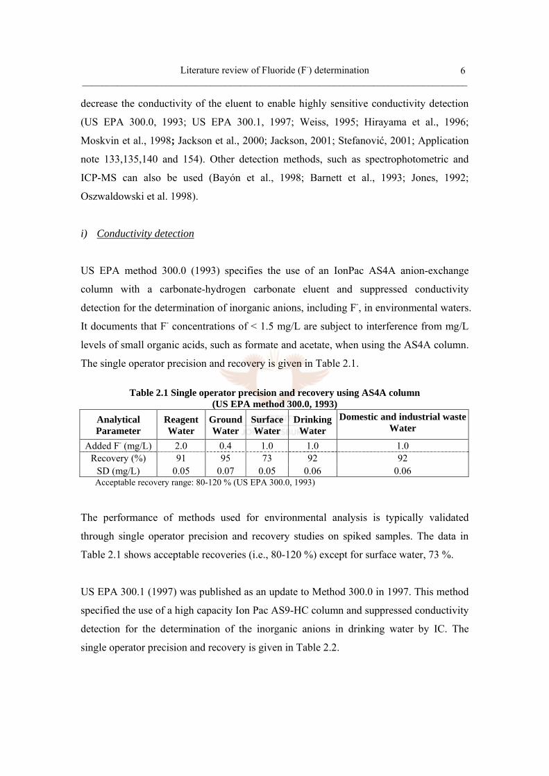
The single operator precision and recovery is given in Table 2.1.
Table 2.1 Single operator precision and recovery using AS4A column
(US EPA method 300.0, 1993) Analytical Parameter
Reagent Water
Ground Water
Surface Water
Drinking Water
Domestic and industrial waste Water
Added F- (mg/L) 2.0 0.4 1.0 1.0 1.0 Recovery (%) 91 95 73 92 92
SD (mg/L) 0.05 0.07 0.05 0.06 0.06 Acceptable recovery range: 80-120 % (US EPA 300.0, 1993)
The performance of methods used for environmental analysis is typically validated
through single operator precision and recovery studies on spiked samples. The data in
Table 2.1 shows acceptable recoveries (i.e., 80-120 %) except for surface water, 73 %.
US EPA 300.1 (1997) was published as an update to Method 300.0 in 1997. This method
specified the use of a high capacity Ion Pac AS9-HC column and suppressed conductivity
detection for the determination of the inorganic anions in drinking water by IC. The
single operator precision and recovery is given in Table 2.2.
Literature review of Fluoride (F-) determination ______________________________________________________________________________
7
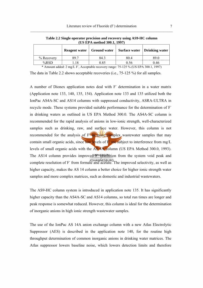
Table 2.2 Single operator precision and recovery using AS9-HC column (US EPA method 300.1, 1997)
Reagent water Ground water Surface water Drinking water
% Recovery 89.7 84.3 80.4 89.0 %RSD 1.18 0.85 0.56 0.46
* Amount added: 2 mg/L F-, Acceptable recovery range: 75-125 % (US EPA 300.1, 1997)
The data in Table 2.2 shows acceptable recoveries (i.e., 75-125 %) for all samples.
A number of Dionex application notes deal with F- determination in a water matrix
(Application note 133, 140, 135, 154). Application note 133 and 135 utilized both the
IonPac AS4A-SC and AS14 columns with suppressed conductivity, ASRA-ULTRA in
recycle mode. These systems provided suitable performance for the determination of F-
in drinking waters as outlined in US EPA Method 300.0. The AS4A-SC column is
recommended for the rapid analysis of anions in low-ionic strength, well-characterized
samples such as drinking, raw, and surface water. However, this column is not
recommended for the analysis of F- in more complex wastewater samples that may
contain small organic acids, since low levels of F- are subject to interference from mg/L
levels of small organic acids with the AS 4A column (US EPA Method 300.0, 1993).
The AS14 column provides improved F- resolution from the system void peak and
complete resolution of F- from formate and acetate. The improved selectivity, as well as
higher capacity, makes the AS 14 column a better choice for higher ionic strength water
samples and more complex matrices, such as domestic and industrial wastewaters.
The AS9-HC column system is introduced in application note 135. It has significantly
higher capacity than the AS4A-SC and AS14 columns, so total run times are longer and
peak response is somewhat reduced. However, this column is ideal for the determination
of inorganic anions in high ionic strength wastewater samples.
The use of the IonPac AS 14A anion exchange column with a new Atlas Electrolytic
Suppressor (AES) is described in the application note 140, for the routine high
throughput determination of common inorganic anions in drinking water matrices. The
Atlas suppressor lowers baseline noise, which lowers detection limits and therefore

Literature review of Fluoride (F-) determination ______________________________________________________________________________
8
improves the detection of trace-level ions. Good long-term performance was realized
using the AS14A with Atlas suppression at 0.8 mL/min.
Traditionally, these columns, AS4A-SC, AS14A and AS9-HC, are designed for use with
carbonate/bicarbonate eluent for determining inorganic anions, including F-, in
environmental samples. A hydroxide-selective column, AS18, which has not been as
widely used for routine analysis of F- due to the lack of appropriate selectivity and
difficulty in preparing contaminant-free hydroxide eluent, has been described for anion
determination. The difficulty in preparing hydroxide eluent is eliminated by using of
automated, electrolytic eluent generation. The AS18 provides improved retention for F-
from the column void volume, overall improved selectivity, and a significantly higher
capacity compared to the AS4A column.
Jackson et al. (2000) tested a modification of Method 300.0 for F- determination. The use
of IC with a hydroxide-selective IonPac AS17 column, automated eluent generation and
potassium hydroxide gradient, was investigated. The AS 17 column provides superior
retention of F- from the column void volume and improved resolution from small organic
acids, such as formate and acetate, compared to the AS 4A column. Jackson (2001)
shows a chromatogram of inorganic anions, of which F- concentration was at 1 mg/L,
obtained using the IonPac AS14A column. No quantification data of F- is provided. The
higher capacity AS14A column provides better overall peak resolution compared to the
AS4A, complete resolution of F- from acetate, and improved resolution of F- from the
void peak.
Stefanović et al. (2001) describes a non-suppressor ion chromatographic method with
conductometric detection for the simultaneous determination of anions, including F-. The
proposed method in this paper shows numerous advantages such as higher selectivity,
shorter analysis time, lower quantitation and detection limits. Moreover, no regeneration
step has to be included and no special equipment is needed. The separation can be
achieved on any liquid chromatograph equipped with a conductometric detector.

Literature review of Fluoride (F-) determination ______________________________________________________________________________
9
The performance of methods used for F- analysis is typically validated through single
operator precision and bias studies on spiked samples. The validity of the method is
established by determining the validation parameter, such as range, linearity, method
detection limit and precision, and the quantitative recovery, obtained from
environmental water matrix. A summary of validation parameters, given in these papers
are tabulated in Table 2.3 and Table 2.4.
Table 2.3 A summary of analytical parameters for F- determination using the IC method
System
aColumn
Range (mg/L)
Linearity(r2)
bMDL (µg/L)
cRt Precision (% RSD)
Area Precision (% RSD)
Reference
DX 120 IonPac AS4A-SC 0.1-100 0.9971 5.9 0.48 0.67
DX 500 IonPac AS 14 0.1-100 0.9980 3.5 0.23 0.17
Dionex dAN 133,135
DX 500 IonPac AS9-HC 0.1-100 0.9980 7.4 0.36 0.58 Dionex
AN135 ICS-2000
Reagent-Free IC
IonPac AS 18 Hydroxide-
selective 0.1-100 0.9991 2.3 0.13 0.27 Dionex
AN154
DX 500 IonPac AS17 Hydroxide-
selective 0.1-100 0.9996 2.9 0.21 0.18 Jackson et al.
2000
Metrohm 690 IC
Metrohm Anion Super
Sep 0.5-50 0.9998 4.0 - - Stefanović et al.,
2001 aColumn : conjunction with relevant guard column bMDL : Method detection limit, cRt : Retention time, dAN: Application Note
The Table 2.3 shows the linear concentration ranges investigated, linearity (r2), and
calculated Method Detection Limit (MDL), which was defined to be the concentration
below which the analytical method cannot reliably detect a response (USEPA, 1984).
The retention time and peak area precision (expressed as % RSD) were determined from
seven replicate injections of a quality control standard, 2mg/L F- solution, as described
in US EPA Method 300.0 (1993) and 300.1 (1997). These results demonstrate that the
hydroxide columns, such as IonPac AS17 and AS 18, which were operated with
electrolytically generated hydroxide eluent, improve the analytical parameters,
compared to conventional IC columns such as the IonPac AS4A, AS 14 and AS 9HC
that use carbonate/bicarbonate eluent.
Literature review of Fluoride (F-) determination ______________________________________________________________________________
10
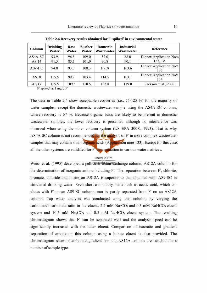
Table 2.4 Recovery results obtained for F- spikeda in environmental water
Column DrinkingWater
Raw Water
SurfaceWater
Domestic Wastewater
Industrial Wastewater Reference
AS4A-SC 93.9 96.5 109.0 57.0 88.0 AS 14 91.5 85.1 101.0 90.8 90.1
Dionex Application Note 133,135
AS9-HC 94.8 93.3 108.3 106.8 103.6 Dionex Application Note 135
AS18 115.5 99.2 103.4 114.5 103.1 Dionex Application Note 154
AS 17 115.5 109.5 110.5 103.8 119.0 Jackson et al., 2000 F- spikeda at 1 mg/L F-
The data in Table 2.4 show acceptable recoveries (i.e., 75-125 %) for the majority of
water samples, except the domestic wastewater sample using the AS4A-SC column,
where recovery is 57 %. Because organic acids are likely to be present in domestic
wastewater samples, the lower recovery is presented although no interference was
observed when using the other column system (US EPA 300.0, 1993). That is why
AS4A-SC column is not recommended for the analysis of F- in more complex wastewater
samples that may contain small organic acids (Application note 133). Except for this case,
all the other systems are validated for F- determination in various water matrices.
Weiss et al. (1995) developed a pellicular anion-exchange column, AS12A column, for
the determination of inorganic anions including F-. The separation between F-, chlorite,
bromate, chloride and nitrite on AS12A is superior to that obtained with AS9-SC in
simulated drinking water. Even short-chain fatty acids such as acetic acid, which co-
elutes with F- on an AS9-SC column, can be partly separated from F- on an AS12A
column. Tap water analysis was conducted using this column, by varying the
carbonate/bicarbonate ratio in the eluent, 2.7 mM Na2CO3 and 0.3 mM NaHCO3 eluent
system and 10.5 mM Na2CO3 and 0.5 mM NaHCO3 eluent system. The resulting
chromatogram shows that F- can be separated well and the analysis speed can be
significantly increased with the latter eluent. Comparison of isocratic and gradient
separation of anions on this column using a borate eluent is also provided. The
chromatogram shows that borate gradients on the AS12A column are suitable for a
number of sample types.
Literature review of Fluoride (F-) determination ______________________________________________________________________________
11
Moskvin et al. (1998) suggested a procedure for preparing an alkaline eluent with low
concentration of F- impurity for the IC determination of weakly retained anions present in
trace amounts in high-purity water. Because of the weak eluent power of OH- ions, the
use of a hydroxide eluent is advantageous only for determining weakly retained ions.
However, hydroxide eluent is difficult to handle, primarily due to the absorption of
carbon dioxide and other acidic gases from air. An anion-exchange purification of the
eluent was designed for extending the analytical range of F- and considerably decreasing
the background electric conductivity of the eluent. The method showed a method
detection limit of 0.05 µg/L at a sample volume of 10 mL.
ii) Spectrophotometric detection
Spectrophotometric methods for the determination of F- are often based on the bleaching
of the colour of various dye complexes, which results in a decrease in their absorbance,
due to the stronger complexes formed between the metal and F- ions (Jones, 1992; Bayón
et al., 1998; Barnett et al., 1993).
Jones (1992) detailed the development of an IC method for the trace determination of F-
in water samples based on the spectrophotometric detection of the AlF2+ species in the
presence of excess Al, 5mg/L, utilizing the post-column formation of an Al complex with
8-hydroxyquinoline sulphonate (8-HQS). This method showed very high sensitivity and
good selectivity. The possible interferences were Zn2+ and Mg2+, overlapping the F- peak,
if present in relatively large amounts, though modification of the eluent and/or post-
column reaction pH can considerably reduce the interferences. The results of F- analysis
for the three samples by the IC and F-ISE methods are in good agreement, yielding
slightly lower level by IC, and certainly within the tolerance of ± 0.1 mg/L F-.
Barnett et al. (1993) presented some results to illustrate the analytical utility of the
zirconyl xylenol orange complex as a post-column reagent for F- detection. A detection
limit of 0.05 µg/mL was achieved with a linear calibration function up to 10 µg/mL. The
Literature review of Fluoride (F-) determination ______________________________________________________________________________
12
observed cationic interferences, such as Mg2+, Ca2+, Al3+ and Fe3+, could be avoided by
the inclusion of a small cation exchange column prior to the analytical column.
Bayón et al. (1999) employed spectrophotometric detection, utilizing a post-column
reaction of the species with 8-hydroxyquinoline-5-sulfonic acid in a micellar medium of
cetyltrimethylammonium bromide. The method for the determination of trace levels of F-
was based on the formation of the AlF2+ complex in excess of Al3+ and separation of the
two species formed (AlF2+ and Al3+) in an ion exchange column. The final determination
was accomplished by post column derivatisation with fluorimetric detection. It showed
good detection limits, but interferences from cations such as Fe3+, Mg2+ and Zn2+ required
the use of the longer CS2 ion exchange column and the addition of EDTA to the sample
solution to eliminate the interferences. However, the chromatogram, obtained for a real
water sample using this condition with photometric detection, yielded 30 minutes Al3+
retention time, while the ICP-MS method, which will be discussed in next paragraph,
showed less than 8 minutes retention time of Al3+. This meant that the photometric
detection was not adequate for F- analysis in the analytical point of view.
iii) ICP-MS detection
ICP techniques have not been used so far for direct F- determination because of the high
excitation and ionization potentials presented by F- which resulted in extremely poor
sensitivity.
Bayón et al. (1998) reported the indirect method for the determination of trace levels of F-
in drinking and seawater samples. It was based on the formation of AlF2+ complex in
excess of Al3+, which allowed complete formation of the AlF2+ complex, and separation
of the two species formed (AlF2+ and Al3+) in an ion exchange column (CG2), after
thermal treatment of the sample for 1h at 50 °C, followed by ICP-MS detection,
monitoring atomic Al at m/z 27. In aqueous acidic solution, Al ions are present as
[Al(H2O)63+], which can react with F- to form the AlF2+ complex. The optimized pH,
where the complex AlF2+ proved to be stable, was 2.6-3. Compared to the
Literature review of Fluoride (F-) determination ______________________________________________________________________________
13
spectrofluorimetric detection method, ICP-MS detection proved to be extremely sensitive,
with a detection limit of 0.1 ng/g of F-, and free from interferences form other cations and
anions in natural water samples. The results obtained for the F- analysis in water samples
using ICP-MS detection were in good agreement with the values found by F-ISE and the
recoveries of 100 ± 10% showed the applicability of the proposed methodology to
perform F- determinations at extremely low levels, at least two orders of magnitude more
sensitive than the ISE method.
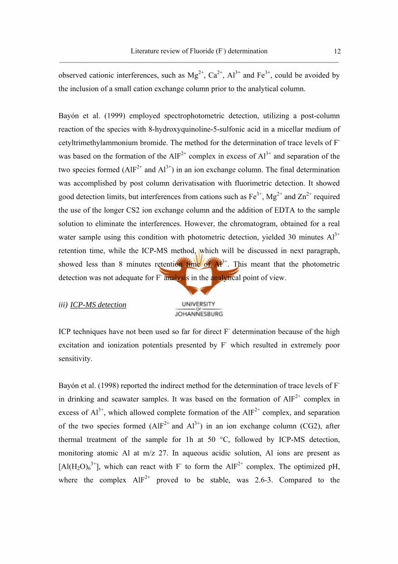
Performance data, using IC method with Spectrophotometric detection and ICP-MS
detection, are summarized in Table 2.5.
Table 2.5 A summary of performance data using spectrophotometric and ICP-MS detectors
Reference and detection method Jones, 1992 Bayón et al. 1999 Barnett et al. 1993Analytical
Parameter Spectro -Photometry
Spectro -Photometry ICP-MS Spectro
-Photometry Post-column
Reagent 8-hydroxyquinoline –5-sulfonic acid
8-hydroxyquinoline –5-sulfonic acid - Zirconyl xylenol
orange Wave
Length 360 nm
And 512 nm 390 nm
And 500 nm - 550 nm
Detection Limit 0.2 µg/L 0.6 ng/mL 0.1 ng/g 0.05 µg/mL
1.2 % (n=6, 50 µg/L) Precision 8.9 % (n=6, 1 µg/L) 2.3 %
(n=5, 20 ng/mL) 4 % -
Linear Range 1-400 µg/L Up to 2000 ng/mL
(Al at 10 ug/g) Up to 100 ng/g (Al at 500 ng/g) Up to 10 µg/mL
Linearity 0.9994 0.9995 0.9993 0.9999
b. Reversed-Phase High Performance Liquid Chromatography (RP-HPLC)
The chromatographic technique, which utilizes a non-polar adsorbent surface and a polar
eluent, has been named Reversed-Phase HPLC (RP-HPLC). Retention is the result of the
interaction of the non-polar components of the solutes and the non-polar stationary phase.
Typical stationary phases are non-polar hydrocarbons, waxy liquids or bonded
hydrocarbons (such as C18, C8, C4, etc.) and the solvents are polar aqueous-organic
mixtures such as water-methanol or water-acetonitrile.
Literature review of Fluoride (F-) determination ______________________________________________________________________________
14
i) RP-HPLC separation with UV-VIS detector
Oszwaldowski et al. (1998) utilized the direct RP-HPLC determination of F-, using a UV-
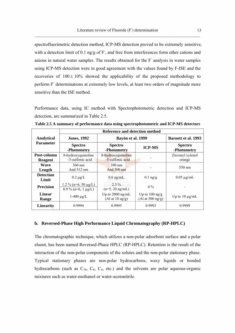
VIS spectrophotometric detector, based on the ternary M-F- -(5-Br-PADAP) complexes
[M=ZrIV or HfIV and 5-Br-PADAP=2-(5-bromo-2-pyridylazo)-5-diethylaminophenol
(Figure 2.1)]. The aim of this paper was to find a ternary coloured system which could
form the basis for a sensitive, selective and rapid chromatographic method. The selected
metal ions, TiIV, VV, NiII, ZnII, ZrIV, NbV, MoVI, SbIII, HfIV, TaV, WVI and UVI, were
examined using spectrophotometry and RP-HPLC over a wide pH range, 2-8, and ZrIV or
HfIV , at pH 4.0 x± 0.3, were found as good ternary coloured systems since these metals
resulted in strong signals, which meant a good sensitivity.
Figure 2.1 5-Br-PADAP
NBr N
N NCH3
CH3HO
Chromatographic separation was performed with C18 end-capped columns, and the eluate
was detected spectrophotometrically at max 585nmλ = . The detection limit in the ZrIV –F- -
(5-Br-PADAP) and HfIV -F- -(5-Br-PADAP), using 20 µL loop, were 0.7 ng/mL and 0.8
ng/mL respectively. Using the proposed methods, F- was determined in tap water based
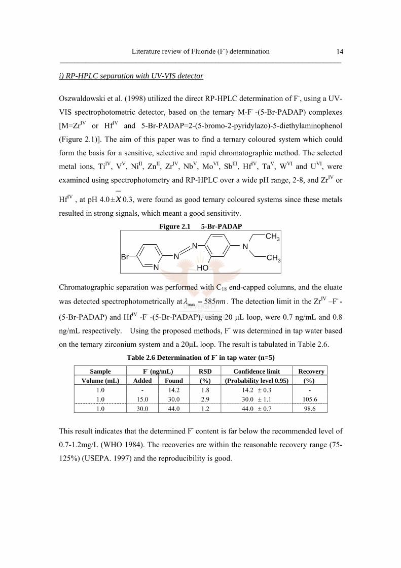
on the ternary zirconium system and a 20µL loop. The result is tabulated in Table 2.6.
Table 2.6 Determination of F- in tap water (n=5)
Sample F- (ng/mL) RSD Confidence limit Recovery Volume (mL) Added Found (%) (Probability level 0.95) (%)
1.0 - 14.2 1.8 14.2 ± 0.3 - 1.0 15.0 30.0 2.9 30.0 ± 1.1 105.6 1.0 30.0 44.0 1.2 44.0 ± 0.7 98.6
This result indicates that the determined F- content is far below the recommended level of
0.7-1.2mg/L (WHO 1984). The recoveries are within the reasonable recovery range (75-
125%) (USEPA. 1997) and the reproducibility is good.

Literature review of Fluoride (F-) determination ______________________________________________________________________________
15
c. Chromatographic F- determination
Up to so far, the chromatographic method with various detection techniques has been
reviewed. A summary of chromatographic conditions for F- determination is given in
Table 2.7.
Table 2.7 A summary of chromatographic condition for F- determination
Column Eluent Fra Iv
b(µL) Detection Reference
IonPac AG4A +AS4A-SC 1.8 mM Na2CO3+ 1.7mM NaHCO3
2.0 50 Conductivity US EPA 300.0, 1993
IonPac AG17+AS17 1-40 mM KOH gradient 2.0 25 Conductivity Jackson et al., 2000 IonPac
AG14A+AS14A 8.0 mM Na2CO3+ 1.0 mM NaHCO3
0.5 25 Conductivity Jackson, 2001
IonPac AG9HC+ AS9HC 9.0 mM Na2CO3 0.4 10 Conductivity US EPA 300.1, 1997
IonPac AG4A+ AS4A-SC
1.8 mM Na2CO3+ 1.7mM NaHCO3
2.0 50 Conductivity
IonPac AG14A+ AS14A
3.5 mM Na2CO3+ 1.0 mM NaHCO3
1.2 50 Conductivity
Dionex Application
Note 133, 135
IonPac AG9 HC+ AS9 HC 9.0 mM Na2CO3 1.0 50 Conductivity
Dionex Application
Note 135
IonPac AG 18+ AS 18
22-40 mM KOH Gradient 1.0 25 Conductivity
Dionex Application
Note 154 Metrohm Anion
Super Sep 1.5-3.5 mM Phtalic acid 1.0-
2.0 100 Conductivity Stefanović et al., 2001
2.7 mM Na2CO3+ 0.3 mM NaHCO3 10.5mM Na2CO3 +0.5mM NaHCO3
IonPac AG 12A+AS12A
20mM Na2B4O7 +18 mM NaOH
1.5 25 Conductivity Weiss et al., 1995
KRS-8P cation guard +KhISK-1 anion analytical column
1 mM NaOH 3.0 250-1000 Conductivity Moskvin et al., 1998
TSKgel IC-Anion-PW
5.0 mM acetylacetone[2,4-
pentanedione]-sodium hydroxide(pH 9)
1.0 100 Conductivity Hirayama et al., 1996
0.1 M K2SO4 (pH 3) 1.0 Spectro- PhotometryIonPac CG2
0.45 M HNO3 0.5100
ICP-MS Bayón et al., 1999
IonPac AS4 5 mM Na2B4O7 (pH 8.2) 1.0 100 Spectro-
Photometry Barnett et al., 1993
IonPac CG2 0.09 M K2SO4 (pH3) 1.0 100 Spectro- Photometry Jones, 1992
C18 end-capped column Acetonitrile-water (85+15 v/v, pH4) 1.0 20 Spectro-
Photometry Oszwaldowski et al., 1998
Fra: flow rate, mL/min, Iv
b: injection volume

Literature review of Fluoride (F-) determination ______________________________________________________________________________
16
2.2.2 Determination of F- by spectrophotometric analysis
Spectrophotometric methods for the determination of F- ion are either based on metal
displacement from a colored complex or the formation of a mixed-ligand complex,
Zr(IV)-F-Alizarin (Standard method, 1955; Crosby et al., 1968), Zr(IV)-F-SPANDS
(Bellack and Schouboe, 1958; Standard method 1975 and 1998; US EPA Method 13 A
and 340.1, 1971; Devine and Partington, 1975; Mac Leod and Crist, 1973; Crosby et al.,
1968), Th(IV)-F-Bromocresol orange (Khalifa and Hafez, 1998), Eriochrome cyanine R
(Crosby et al., 1968), Semi-Methylthymol Blue (SMTB), Semi-Bromocresol Orange
(SBCO), Methylnaphthlo Orange (MNO), Naphthol Violet (NV) (Yuchi et al., 1995).
This method is subject to much interference, most of which are supposed to be eliminated
by the preliminary distillation step (Standard method 1975; Standard method 1998; US
EPA Method 13 A and 340.1, 1971) or micro diffusion (Sara 1975).
Water samples were analyzed for F- by one of the several alizarin-zirconium methods,
either visually or by using a colorimeter (Standard Method, 1955). These methods had a
serious drawback in that the colour development is progressive, requiring accurate timing
to achieve consistent results. The waiting period was also a source of constant annoyance.
The distillation step was necessary to avoid interferences.
Bellack and Schouboe (1958) developed a simple and rapid SPANDS (2-(para-
sulfophenylazo)-1,8-dihydroxynaphthalene-3,6-disulfonate) method, in place of the usual
alizarin-zirconium photometric methods, which yielded an accuracy within 0.02 mg/L in
the F- concentration range of 0.00 to 1.40 mg/L. Compared to alizarin-zirconium methods,
it saved considerable time and increased precision. It was, however, still subject to many
interferences, so that the distillation step had to be applied to eliminate interferences. A
distillation step severely restricts the number of samples that can be analysed in a given
period, so that this distillation step is often omitted when large numbers of samples have
to be analysed (Harwood, 1969). The SPANDS method became the reference
spectrophotometric method for the F- analysis in water. (Bellack and Schouboe, 1958;
Standard method 1975 and 1998; US EPA Method 13 A and 340.1, 1971).
Literature review of Fluoride (F-) determination ______________________________________________________________________________
17
Leod and Crist (1973) stated that although the SPANDS method was generally regarded
as accurate and sensitive, it was extremely time consuming requiring a sulfuric acid or
perchloric acid distillation step to remove interferences. This paper describes the results
of a study to assess the equivalence of the ISE and SPANDS methods for the
determination of soluble F-. The data presented in this paper indicate that the
determination of F- by the ISE gives results which are essentially equivalent to the
SPANDS method and require much less analysis time. The conclusion of this paper is
that the ISE method offers a number of significant advantages over the SPANDS method
by virtue of its simplicity, high precision, and speed. Devine and Partington (1975) also
suggests that the F-ISE method following distillation be adopted as the method of choice.
They found that serious errors have been experienced in the analysis of wastewater
samples for F- concentration by the SPANDS spectrophotometric method. The source of
positive interference in this method was due primarily to sulfate ion carry-over during the
preliminary distillation step. The chemical analysis of F- in water is subject to many
errors, due to interference of constituents present in the water. A distillation step is
therefore often included in the procedure to remove these interferences.
Crosby et al. (1968) evaluated four of the most frequently used reagents, such as Alizarin
red S, Eriochrome cyanine R, SPANS and Alizarin complexone, for the F- determination
in water with respect to reproducibility, sensitivity, range, stability of colored products
and of reagents, specificity and effect of temperature. The Alizarin complexone
procedure had many advantages over the spectrophotometric method, and was
particularly suitable for samples containing only very small amounts of F-. The analytical
results of F- determination from the spectrophotometric method and those from the ISE
method are compared and the F-ISE surpasses all the spectrophotometric methods with
regard to speed, accuracy and convenience, and is recommended for the routine
monitoring of fluoridated water supplies.
Complexes of tetravalent metal ions, such as zirconium (IV), thoruim (IV) and hafnium
(IV), with chromogenic chelating reagents having only one methyliminodiacetated group
Literature review of Fluoride (F-) determination ______________________________________________________________________________
18
ortho to the OH group were examined for spectrophotometric determination of F- by
Yuchi et al. (1995). Several compounds [Semi-Methylthymol Blue (SMTB), Semi-
Bromocresol Orange (SBCO), Methylnaphthlo Orange (MNO), Naphthol Violet (NV)]
have been examined for the validity of the improvement in sensitivities of
spectrophotometric determination of F-. Zirconium (IV) and hafnium (IV) were superior
to thorium (IV) as a central metal ion. The reaction with F- in this study was described as
follows:
Zr2(OH)4(HL)2+2F- ↔ 2ZrLF +2OH- + 2H2O
Khalifa and Hafez (1998) investigated the ternary purple coloured complex formed
between Th4+, bromocresol orange (BCO) in acidic medium. A spectrophotometric
method, based upon the decrease in colour intensity of the Th-BCO complex on mixing it
with F- ion, is also described. The proposed method was convenient, rapid and sensitive
for F-, and could be used for the determination of F- in the 0.02-3.00 µg/mL ranges with
standard deviation ±0.9 %. 2.2.3 Determination of F- by micro fluidic analysis (FIA, SIA) a. Introduction
Microfluidics for automated sample processing can be based either on continuous flow,
such as Flow Injection Analysis (FIA), or on programmable flow, such as Sequential
Injection Analysis (SIA). FIA uses constant forward motion of the carrier to transport
sample from injector to detector. The reagents are added continuously to the carrier
stream near the injection zone and samples are injected into a carrier/reagent solution,
allowing the sample and reagent to mix, which transports the sample zone into a detector
while desired chemical reactions take place. The resulting reaction product forms a
concentration gradient corresponding to the concentration of the analyte throughout the
entire sample zone length. SIA, on the other hand, uses flow reversals, and flow
acceleration to mix sample with reagents, and stop flow to accommodate reaction time,
and to monitor the reaction rate based response. The advantage of FIA is transparency of
Literature review of Fluoride (F-) determination ______________________________________________________________________________
19
operation, while SIA is more versatile and that a reduced sample and reagent volume are
required since sample manipulation is automated.
b. Flow Injection Analysis (FIA)
i) Potentiometric detector (ISE)
The F-ISE has been widely used as a detector in FIA because of its simplicity, selectivity
and relatively low cost. Extensive studies concerning the use of F-ISE in FIA have been
performed by various research groups (Slanina et al., 1980; Trojanowicz and
Matuszewski, 1982; Frenzel and Brätter, 1986; Najib and Othman, 1992; Borzitsky et al.,
1993). The advantages associated with the coupling of the F-ISE as sensor to an FIA
system, enables this combination to be used in a reliable low cost, robust analyzer for the
determination of F- in toothpaste as well as in effluent streams, natural and borehole
water samples. By using FIA systems, the selectivity of the electrode is improved due to
the very short contact time of the interfering ions with the electrode membrane. The
application of the F- analysis in water samples are reported by several authors (Frenzel
and Brätter, 1986; Wang et al., 1995; Trojanowicz et al., 1998; Papaefstathiou et al.,
1995; Lopes da Conceição et al. 2000; Stefan et al. 1999).
The F-ISE has been widely used for monitoring F-, but its application in FIA systems has
been limited because of its memory effect (Slanina et al., 1980; Trojanowicz and
Matuszewski, 1982). Van Oort and Van Eerd (1983) obtained a fast response from the F-
ISE in a FIA system by using a mixture of methanol and total ionic-strength adjusting
buffer containing 10-6M F- in the carrier and by polishing the electrode surface with fine
wet alumina powder. However, no application to real samples was presented.
Frenzel and Brätter (1986) employed the FIA with a combination F-ISE, yielding an
excellent sensitivity down to 1ug/L, to the determination of traces of F- in tap water.
However, for the analysis of samples with high inherent ionic strength and fairly large
amounts of interfering elements, the optimization of the particular TISAB was necessary.
Literature review of Fluoride (F-) determination ______________________________________________________________________________
20
Emphasis was laid on the requirement for particular TISAB solutions to obtain accurate
results at low F- levels. The citrate TISAB was found to be effective to overcome the
interferences, but it reduces the sensitivity and causes peak broadening when compared to
the commonly used TISAB III. Recoveries after spiking tap water with F- concentrations
ranging from 0.01 to 1 mg/L were in the range 91-106 %.
Although the ISE detector has merits, such as simplicity, selectivity and low cost, one of
the major inconveniences in the applications, however, is its relatively slow response in
solutions of low F- ion concentration. Wang et al. (1995) aimed to establish a simple and
fast method, overcoming the pitfall, for determining low F- concentration using FIA by
applying an extrapolation procedure to predict the electrode equilibrium potential,
without the necessity of waiting for the establishment of the steady-state.
This work clearly showed that FIA with the extrapolation method was faster compared
with the conventional method, and had higher sensitivity. And also the accuracy of the
method was good, making it particularly suitable for the determination of large numbers
of samples at low F- concentration, such as in environmental analysis.
Stefan et al. (1999) reported on the incorporation of F-ISE in an FIA system for the
determination of F- in effluent streams, natural and borehole water. This system was
suitable for the on-line monitoring of F- at a sampling rate of 60 samples/h in the linear
range 10-4-10-1 (approximately 1.9-1900 mg/L) with an RSD of better than 0.6 %. But the
disadvantage of the proposed method was the relatively high detection limit of 0.34 mg/L.
Lopes da Conceição et al. (2000), proposed the use of the entire time-dependent response,
instead of the final potential reading alone (Trojanowicz et al. (1998), as an improved ion
activity assessment with ISE and a flow through system. They explored the concentration
gradient in a flow injection system for the potentiometric determination of F- in water
samples based on a gradient flow injection titration. Determination of F- is accomplished
by switching the injection valve between a standard and a sample solution. The
methodology developed gave results with a relative standard deviation of about 3 %,
Literature review of Fluoride (F-) determination ______________________________________________________________________________
21
detection limit of 0.19 mg/L, and the average recoveries after spiking natural samples
with F- were in the range 100-102%.
ii) Spectrophotometric detector
The FIA method for the F- determination using spectrophotometric detection can be
applied either without pretreatment (Wada et al., 1985; Arancibia et al., 2004) or with
pretreatment such as extraction (Garrido et al., 2002), gas diffusion (Fang et al., 1988;
Cardwell et al., 1994).
• Without pretreatment
Wada et al. (1985) reported the spectrophotometric determination of F- in the range of
0.03-1.2 mg/L, with lanthanum/alizarin complexone (1:1) in 70 % acetone by the FIA
method, in conjunction with a 500 cm reaction coil at 60°C at 24 samples per hour. This
method was applied to tap water samples, using standard addition method.
The presence of high sulphate constitutes a serious interference in the SPANDS method
for the determination of F- in water. Thus, Arancibia et al. (2004) explored the Zr-
SPANDS method incorporating full spectral measurements and a suitable multivariate
calibration methodology. Partial least-squares (PLS) regression appeared to be the
candidate of choice, due to the quality of its predictive models, the availability of
software and the ease of its implementation. They combined this strategy with flow
injection analysis, in order to develop an automated method for routine F- monitoring. By
coupling the FIA system to a diode-array spectrophotometric detector it is possible to
obtain the spectra from the recorded FIA peaks. The comparison between the obtained
results by using the FIA/PLS method and those obtained with an ISE showed a good
agreement.
• With pretreatment
1) Gas diffusion
Literature review of Fluoride (F-) determination ______________________________________________________________________________
22
Many reports have appeared on the use of gas diffusion (GD) in flow injection analysis
for different gaseous species but few have given details of this methodology for the
analysis of F-. Fang et al. (1988) gives a detailed description of an automated GD-FIA
method. This procedure involved separation and on-line preconcentration of the F-. The
sample was acidified and heated to 78°C while passing through a coil. HF formed in the
donor stream, diffused through a Teflon membrane in the gas diffusion unit to be
preconcentrated for a set time period in a static alkaline recipient solution enclosed in the
sample loop of an injection valve. At the end of that time, the injector was activated and
the carrier transported the absorbed sample down-stream where it merged with
lanthanum/alizarin complexone solution to be determined spectrophotometrically at 620
nm. F- was determined in wastewater at a sample rate of 40/hr with a detection limit of
0.1 mg/L. Al still interfered but there was considerable improvement in the concentration
of Al ion, which could be tolerated in the system, compared with that by the direct
spectrophotometric procedure without separation by gas diffusion.
Cardwell et al. (1994) shows the application of the GD, as a pre-treatment technique, with
the FIA method prior to spectrophotometric detector. The pre-treatment of F- was
achieved on-line by converting it to trimethylsilane, which then diffuses through a gas
permeable membrane to be absorbed in a stationary sodium hydroxide acceptor stream.
This stream was enclosed in the sample loop of an injection valve and after pre-treatment,
the F- sample was flushed into a flow injection manifold for spectrophotometric analysis
by the zirconium/alizarin procedure at 520 nm. The method was suitable for F- analysis in
the range 0.1-10 mg/L at a sampling rate of 17/hour. The detection limit was calculated to
be 0.055 mg/L and the quantification limit was found to be 0.18 mg/L. The accuracy and
precision of the method for real water samples, collected from boreholes, a drainage farm,
reservoirs and reticulation sites, have proven to be comparable with the F-ISE batch
method for the samples tested. The results obtained by the FIA method correlated well
with those obtained by the F-ISE method, giving a correlation coefficient of 0.9970.
2) Solid phase extraction (SPE)

Literature review of Fluoride (F-) determination ______________________________________________________________________________
23
Garrido et al. (2002) suggested a spectrophotometric determination of F- in a flow
assembly integrated on-line to an open/closed FIA system to remove interference by solid
phase extraction. The method is based on the enhanced fluorescence of quercitin-Zr (IV)
complex when F- ion is present in the sample. An open/close FIA manifold with a mini-
column of Dowex 50W X8 resins was used to remove the most important interference of
aluminium. The proposed method was applied for F- determination in several water
samples and the results compared with the SPANDS method. Good agreement between
the two methods was obtained.
c. Sequential Injection Analysis (SIA)
i) Potentiometric detector (ISE)
Applications of SIA to environmental analysis is an attractive field due to the ability to
perform multicomponent determinations using several chemical reactions involving
various reagents in different zones, various types of detectors or even diverse multivariate
techniques. Specifically, SIA can be used to obtain necessary control measurements of
water in a rapid and simple way. Alpízar et al. (1996) illustrated the possibility of SIA
on-line implementation with potentiometric detection for simultaneous chloride and F-
determination in waters, using two ion selective electrodes in two serial flow-through
cells. The necessary ionic strength adjustment was obtained by mixing the TISAB
solution with the sample by diffusion during the propelling process to the detection cells.
The proposed method gave results with a relative standard deviation of 3.7 % at 1µg/mL
F- and the average recoveries after spiking tap water samples with F- were in the range
92-109%. This methodology was applied successfully to drinking tap water samples.
The versatility of the SIA technique is centered on a selection valve where each port of
the valve allows a different operation to be performed. Van Staden et al. (2000)
investigated the peak profiles of four different buffer-sample SIA configurations, e.g.
buffer-sample; sample-buffer; buffer-sample-buffer and sample-buffer-sample, with a F-
ISE and the application to the determination of F- in tap water. The best response
Literature review of Fluoride (F-) determination ______________________________________________________________________________
24
characteristics and peak shapes as well as recovery and precision values were obtained
for the buffer-sample configuration.
2.2.4 Determination of F- by potentiometric analysis The potentiometric technique, mainly F-ISE, is considered the simplest and most reliable
for F- determination (Durst, 1969; Fry and Taves, 1970; Hall et al., 1972; Hallsworth et
al., 1976; Retief et at., 1985; Kissa, 1987; Villa, 1988; Vogel et al., 1990). The F-ISE
method for the F- determination can be applied either without pretreatment technique,
namely conventional potentiometric method, (Babcock and Johnson, 1968; Frant and
Ross, 1968; Harwood, 1969) or with pretreatment technique, the extended method, such
as co-precipitation (Okutani et al., 1989) and steam distillation (Analytical working group,
1986).
a. Conventional potentiometric method
Babcock and Johnson (1968) used the electrode without the addition of any ionic buffer
for the determination of F- in municipal water. Their particular application was basically
that of monitoring a municipal water supply for F-. Under such conditions, the
composition of the water, and hence the total ionic strength, would remain fairly constant
since the water originated form the same source. Consequently there was no great
necessity to add electrolytes to ensure constant ionic strength.
Frant and Ross (1968), on the other hand, have used the electrode on samples from
different sources, and so had to make use of an ionic buffer. This method was selected for
routine F- analysis. Later tests indicated that the composition of the ion buffer should be
changed in order to overcome interference from aluminium. Results obtained indicate
that with the new ionic buffer, satisfactory analysis for F- can be obtained even in the
presence of up to 5 mg Al /L.
Crosby et al. (1968) evaluated ISE method and five spectrophotometric procedures for
the determination of F- in potable waters and other aqueous solutions, with respect to
Literature review of Fluoride (F-) determination ______________________________________________________________________________
25
reproducibility, sensitivity, range, stability of coloured products and of reagents,
specificity and effect of temperature. F- was determined directly, without the need for any
separation step. The ISE method was shown to be less susceptible than the colorimetric
methods to interference from other ions in solution.
Harwood (1969) evaluated a commercially available F-ISE for use in routine F-
determination on water samples. Tests on samples showed that aluminium interfered
seriously and an ionic buffer containing CDTA was recommended in order to control this
interference, since both citrate and EDTA had only limited applicability. With CDTA
present, reliable F- determination were possible in the presence of up to 5 mg/L
aluminium. The F- analysis results were compared using both SPANDS method and ISE
and the results, obtained with the F-ISE, were more trustworthy because of the inherent
difficulties of the SPANDS method.
b. Extended potentiometric method
i) Co-precipitation
Okutani et al. (1989) performed the F- determination in natural water, such as sea, tap,
well and river waters, using F-ISE after co-precipitation with aluminium phosphate. The
value, obtained by the proposed method, agreed well with those obtained by IC.
ii) Steam distillation
The analytical working group of the comité technique européen du fluor (1986)
determined the F- in rain water and aqueous effluents using both direct potentiometric and
extended potentiometric methods. All the methods are based on final measurement of F-
by means of the F-ISE. Interferences which could not be eliminated by the masking
power of the TISAB buffer solution (1M sodium chloride and 0.1 M citrate buffer at pH
5.5) were avoided by separation of F- by steam distillation. F- was distilled from a
mixture of perchloric and phosphoric acid. Several samples of waste water were
Literature review of Fluoride (F-) determination ______________________________________________________________________________
26
determined by using both methods, and the results showed that the extended method
yielded satisfactory results.
2.2.5 Other methods
a. Pervaporation
Pervaporation is an energy efficient combination of membrane permeation and
evaporation and is considered an attractive alternative for many separation
processes. The process, which requires only low temperatures and pressures, has cost
and performance advantages compared with distillation for constant-boiling
mixtures. Pervaporation is particularly suitable for the dehydration of organic solvents
and the removal of organics, such as methanol and acetone, from aqueous streams. In the
pervaporation process the liquid (mixture) is in contact with the membrane. At the
permeate side, a partial pressure is generated by means of a vacuum pump, or by means
of an inert gas flow. The components of the liquid that move through the membrane are
vaporized by the low pressure, removed and condensed.
Papaefstathiou et al. (1995) developed a selective method for the determination of F- in
contaminated samples based on pervaporation of a volatile derivative and potentiometric
monitoring of the anion after collection in a basic solution. F- was converted to volatile
trimethylfluorosilane by reaction with hexamethyldisilazane, and absorbed in dilute
NaOH solution. Both the continuous and stopped-flow modes were used in order to
accomplish a variable efficiency of the separation process thus enlarging the
determination range which was established between 5 and 100 mg/L. The precision was
between 2.60 and 3.58 %. The determination of the analyte in samples from different
sources, such as tap water, well water, fertilizers and ceramic industry wastewater,
testified to its usefulness, giving the recovery range between 87.23 and 106.09% with
RSD values between 0.72 and 4.17 %.
b. Extraction
Literature review of Fluoride (F-) determination ______________________________________________________________________________
27
Extraction is primarily used to separate analytes from a matrix thus eliminating or
reducing interferences from other components. Secondly, it is used to concentrate the
analyte up to a detectable concentration level.
Nishimoto et al. (2001) employed spectrophotometry after solvent extraction of F- into
chloroform using [2,23-diethy-8,17-bis(2-ethoxycarbonylethyl)-3,7,12,13,18,22-
hexamethylsapphyrin (H3 sap), sapphyrin] in the presence of 0.1 M sodium nitrate. F- ion
was extracted from chloroform with the positively charged sapphyrin, as ion-pair
complexes of H5sap2+·F-·NO3-, that gave a new absorption maximum wavelength at 448
nm. The results provided the determination of F- ion at concentrations as low as 0.01
mg/L. Metal ions like Al(III) and Fe(III) did not interfere with the determination of F-.
2.2.6 Comparative studies
The references to results of comparative studies are summarized in Table 2.8.
Table 2.8 A summary of comparative study of F- analysis
Comparison method Reference Section Spectrophotometry ISE Crosby et al. (1968) 2.2.2, 2.2.4.a
SPANDS ISE Harwood (1969) 2.2.4.a SPANDS ISE Leod and Crist (1973) 2.2.2
GD-FIA ISE Cardwell et al. (1994) 2.2.3.b.ii 2.2.4.a
IC ISE Van den Hoop et al. (1996) 2.2.4.a
SPANDS Solid Phase Extraction Garrido et al. (2002) 2.2.3.b.ii
FIA/PLS ISE Arancibia et al. (2004) 2.2.3.b.ii 2.2.4.a

Theory of analytical methods ______________________________________________________________________________________
28
Chapter 3 Theory of analytical methods
3.1 Ion Selective Electrodes (ISE)
3.1.1 Introduction
The Ion Selective Electrode (ISE) is a sensor for the potentiometric determination of
ionic species and one of the most frequently used devices during laboratory analysis in
industry, process control, physiological measurements, and environmental monitoring.
The functioning of an ISE is based on the selectivity of passage of charged species from
one phase to another, leading to the creation of a potential difference. The most
commonly used ISE is the pH probe. Other ions that can be measured include anions such
as, F-, Br-, I-, CN-, NO3-, NO2
-, the cations such as, Pb2+, K+, Ca2+, Cu2+ and Na+, and
gasses in solution such as NH3, CO2, N2 and O2.
Some advantages of the ISE method are:
• It is considerably less expensive than other analytical techniques, such as Atomic
Adsorption Spectrophotometry (AAS) or Ion Chromatography (IC).
• It is simple to use and measurement is quick.
• It has a large range of applications and can be used over a wide concentration
range.
• It is robust and durable and ideal for use in either field or laboratory environments.
• Accuracy and precision levels of ± 2% for some ions compare favourably with
analytical techniques which require more complex and expensive instrumentation.
3.1.2 Important concepts of ISE (Skoog et al., 1997)

Theory of analytical methods ______________________________________________________________________________________
29
a. Activity
Activity is the effective concentration of a free ion in a solution. It is dependent on the
total ionic strength of a solution. In dilute solutions with low ionic strength, the ions are
relatively far apart and free to move so that the activity and concentration are virtually
identical. In more concentrated solutions, or high ionic strength, however, the ions are
more closely packed and their charges are shielded. Thus activity may differ from
concentration and is usually lower up to ionic strengths of about 0.1 M. In solutions with
concentrations of more than 1 M other interactions such as hydration and inter-ionic
interactions, which can impede movement, become important, and activity can actually
be larger than the concentration. In the case of ISE measurements, the activity of the
measured ion determines the proportion of ions passing through the ion-selective
membrane and thus the magnitude of the voltage developed by the electrode.
The activity of an ion in solution for any known concentration may be calculated from
the formula:
x xa Cγ= × (3.1) Where, xγ is the activity coefficient and C is the Molar concentration
i) Ionic strength (µ)
The ionic strength of a solution is a measure of the total effect of all the ions, both
positive and negative, present in the solution and is given by the equation:
20.5 i ii
C Zµ = ×∑ (3.2)
Where, Ci = the species molar concentration Zi = charges of ions
ii) Activity coefficient
The activity coefficient is dependent on the ionic strength of the solution. It becomes
progressively lower as the ionic strength increases, due to inter-ionic interactions. The
activity coefficient for any ion in solution can be calculated using the Debye-Hückel
equation that permits the calculation of activity coefficients of ions from their charge and
their average size.
Theory of analytical methods ______________________________________________________________________________________
30
-Log xγ = µαµ
x
xZ3.31
51.0 2
+ (3.3)
Where: Z x = the ionic charge, µ = the ionic strength of the solution αx = effective diameter of the hydrated ion X in nanometers (10-9m), approximately 0.3nm for most singly charged ions. The constants 0.51 and 3.3 are applicable to aqueous solutions at 25 °C
In solutions of very low ionic strength, when µ is less than 0.01, the denominator of the
equation becomes 1 and the equation can be simplified to:
-Log xγ = 0.51 Zx2 µ (3.4)
b. Nernst equation
This is the fundamental equation, which relates the electrode potential to the activity of
the measured ions in the test solution.
log0592.0n
EE −°= (a) (3.5)
Where, E = the total potential (in mV) developed between the sensing and reference electrodes E0 = a constant which is characteristic of the particular ISE/reference pair n = the charge on the ion (with sign) Log (a) = the logarithm of the activity of the measured ion
Note that the activity is equivalent to the concentration in dilute solutions but becomes
increasingly lower as the ionic strength increases. This is effectively the equation of a
straight line:
y mx c= + (3.6)
Where, y = E = the measured electrode response in mV, x = Log (a), c = E0 = the intercept on the y axis. m = -0.0592/n = the slope of the line (the electrode slope)
An electrode is said to have a Nernstian response over a given concentration range if a
plot of the potential difference versus the logarithm of the ionic activity of a given
species in the test solution, is linear with a slope factor that is given by the Nernst
equation.
Theory of analytical methods ______________________________________________________________________________________
31
c. Range of linear response
At high and very low ion activities there are deviations from linearity. Typically, the
electrode calibration curve exhibits linear response range between 10-1M and 10-5M.
d. Slope
The slope of an electrode is the gradient of the line formed by plotting the electrode
response in millivolts against the logarithm of the activity (or concentration) of the
measured ion. The theoretical Nernstian slope at 25°C is 59.16 mV/decade change in
activity for monovalent ions and 29.58 mV/decade for divalent ions. In practice the slope
is generally lower than this theoretical value due to inefficiency of the ion selective
membranes and failure to meet ideal conditions.
Measured slopes generally lie in the range 54±5 and 26±3 respectively.
e. Liquid junction potential
Liquid junction potential is the potential formed at the interface between any two-
electrolyte solutions of different compositions. In ISE measurements, the most important
liquid junction is that between the reference electrode filling solution and the sample
solution. Ideally, this potential should be as low and as constant as possible, despite
variations in the external solution. Reference electrode filling solutions are chosen to
minimize this potential.
f. Hysteresis (electrode memory)
The occurrence of a different value in the potential difference after the concentration of
the test solution has been changed and then restored to its original value. This systematic
error is generally in the direction of the concentration of the previous solution. Thus, if
the electrodes are washed with water between each sample measurement, successive
readings of the same solution can be expected to become progressively lower for cation
and higher for anions.
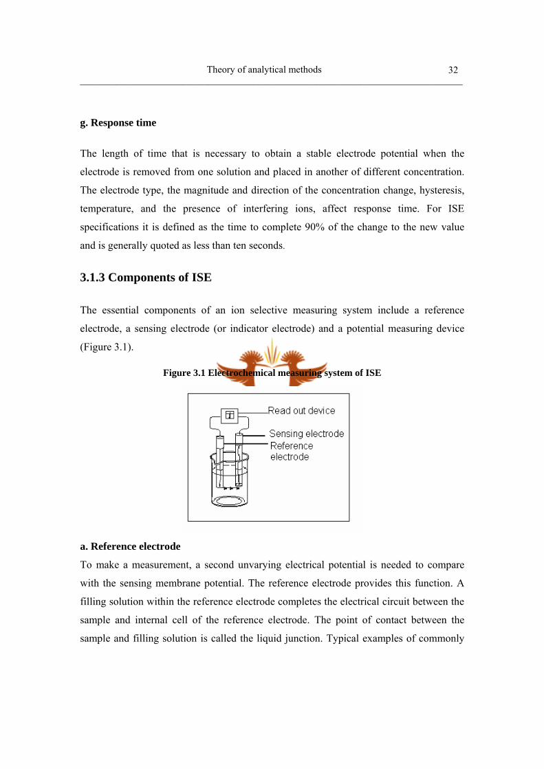
Theory of analytical methods ______________________________________________________________________________________
32
g. Response time
The length of time that is necessary to obtain a stable electrode potential when the
electrode is removed from one solution and placed in another of different concentration.
The electrode type, the magnitude and direction of the concentration change, hysteresis,
temperature, and the presence of interfering ions, affect response time. For ISE
specifications it is defined as the time to complete 90% of the change to the new value
and is generally quoted as less than ten seconds.
3.1.3 Components of ISE
The essential components of an ion selective measuring system include a reference
electrode, a sensing electrode (or indicator electrode) and a potential measuring device
(Figure 3.1).
Figure 3.1 Electrochemical measuring system of ISE
a. Reference electrode
To make a measurement, a second unvarying electrical potential is needed to compare
with the sensing membrane potential. The reference electrode provides this function. A
filling solution within the reference electrode completes the electrical circuit between the
sample and internal cell of the reference electrode. The point of contact between the
sample and filling solution is called the liquid junction. Typical examples of commonly

Theory of analytical methods ______________________________________________________________________________________
33
used reference electrodes are the calomel electrodes and the silver/silver chloride
electrodes.
i) Silver/silver chloride electrode
It is the most common and simplest reference system. This generally consists of a
cylindrical glass tube containing a 4 M solution of KCl saturated with AgCl. In
electrochemical terms, the half-cell can be represented by:
Ag | AgCl (Satd), KCl (Satd) || (3.7)
And the electrode reaction is:
AgCl (s) + e- ↔ Ag (s) + Cl- (aq) (3.8)
The electrode potential for this half-cell is + 0.2046 V relative to the Standard Hydrogen
Electrode at 25°C
ii) Calomel electrode
It consists of mercury in contact with a solution that is saturated with mercury (I) chloride
and also contains a known concentration of KCl. In electrochemical terms, the half-cell
can be represented by:
Hg | Hg2Cl2 (Satd), KCl (xM) || (3.9)
Where, x is the molar concentration of KCl
And the electrode reaction is:
Hg2Cl2 (s) + 2e- ↔ 2Hg (l) + 2Cl- (aq) (3.10)
The electrode potential for this half-cell is + 0.2444 V relative to the Standard Hydrogen
Electrode at 25°C.
b. Sensing electrode (indicator electrode)

Theory of analytical methods ______________________________________________________________________________________
34
Membrane electrodes are called ion selective electrodes because of their high selectivity.
The membranes must have minimal solubility, electrical conductivity, and selective
reactivity with the analyte of interest. Several types of sensing electrodes are
commercially available (Orion Research). Table 3.1 shows different types of ISE and
some of the analytes they are used for.
Table 3.1 Types of ion selective membrane electrode
Types Example
Single crystal LaF3 for F- Crystalline membrane electrode Polycrystalline or mixed
crystal Ag2S for S2- and Ag+
Glass Silicate glasses for Na+ and H+
Liquid Liquid ion exchangers for Ca2+ and neutral carriers for K+
Noncrystalline membrane electrode
Immobilized liquid in a rigid polymer
Polyvinyl chloride matrix for Ca2+ and NO3
-
Attention will be focused on crystalline membrane electrodes used for the determination
of fluoride (F-), since F- is the target element of this study.
3.1.4 Fluoride ion selective electrode
a. Introduction
The F- Ion-Selective Electrode is designed for the detection of F- in aqueous solutions and
is suitable for use in both field and laboratory applications. The F- electrode consists of a
solid-state inorganic membrane of LaF3 crystal, bounded into an epoxy body (Figure 3.2).
Figure 3.2 Construction of fluoride electrode
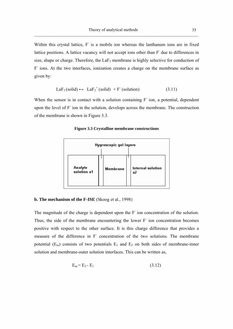
Theory of analytical methods ______________________________________________________________________________________
35
Within this crystal lattice, F- is a mobile ion whereas the lanthanum ions are in fixed
lattice positions. A lattice vacancy will not accept ions other than F- due to differences in
size, shape or charge. Therefore, the LaF3 membrane is highly selective for conduction of
F- ions. At the two interfaces, ionization creates a charge on the membrane surface as
given by:
LaF3 (solid) ↔ LaF2+ (solid) + F- (solution) (3.11)
When the sensor is in contact with a solution containing F- ion, a potential, dependent
upon the level of F- ion in the solution, develops across the membrane. The construction
of the membrane is shown in Figure 3.3.
Figure 3.3 Crystalline membrane constructions
b. The mechanism of the F-ISE (Skoog et al., 1998)
The magnitude of the charge is dependent upon the F- ion concentration of the solution.
Thus, the side of the membrane encountering the lower F- ion concentration becomes
positive with respect to the other surface. It is this charge difference that provides a
measure of the difference in F- concentration of the two solutions. The membrane
potential (Em) consists of two potentials E1 and E2 on both sides of membrane-inner
solution and membrane-outer solution interfaces. This can be written as,
Em = E2 - E1 (3.12)

Theory of analytical methods ______________________________________________________________________________________
36
The F- ion activities at each face are related to the Nernst–like relationships.
E1 = j1-1
1'log0592.0aa
n (3.13)
E2 = j2-2
2 'log0592.0aa
n (3.14)
Where, j1 and j2 are constants and a1 and a2 are activities of F- in the solutions on the
external and internal sides of membrane respectively. The terms a1’ and a2’ are the
activities of F- at the external and internal surfaces of the membrane. Since the two
membrane surfaces are usually identical, so j1 and j2 as well as a1’ and a2’ are also
identical. By substituting two equations and employing the equalities j1 = j2, a1’ = a2’ and
n=1, the membrane potential (Em) can be rearranged like,
Em = E2 - E1 = 0.0592 log 1
2
aa (3.15)
Thus, the membrane potential Em depends only on the F- ion activities of the solutions on
either side of the membrane. For an ISE, the ion activity of the internal solution a2 is a
constant at temperature 25 °C, the equation can be simplified and the potential of a cell
containing a lanthanum F- electrode is given by the equation to
Em = L + 0.0592 logaF- = L - 0.0592 pF- (3.16)
Where, L = 0.0592 log a2
The net potential is measured against a reference electrode.
Ecell = Eise – Eref (3.17)
The results are usually given in milli volts or even directly as concentrations of the
species being measured. The strength of this charge is directly proportional to the
concentration of the selected ion.
Theory of analytical methods ______________________________________________________________________________________
37
c. Total Ionic Strength Adjustment Buffer (TISAB) for F-ISE (Front and Ross, 1968;
Durst, 1969)
The problems with Ion Selective Electrode measurements are the effect of interferences
from other ions in solution, the effect of the ionic strength of the solution reducing the
measured activity relative to the true concentration at high concentrations. TISAB (Total
Ionic Strength Adjustment Buffer) is normally added to samples and standards in order to
solve these problems. The function of the TISAB is discussed below.
i) Adjustment of a constant ionic strength for both standards and samples
As discussed in Section 3.1.2.a, the F- electrode actually measures activity. The measured
result is therefore strongly dependent on the ionic strength of the medium. TISAB
ensures a constant ionic strength background, minimizing variations between samples
and standards, which may otherwise influence the electrode potential. A constant ionic
strength also reduces errors due to liquid junction potentials (Butler, 1969).
ii) Optimization of the pH
Of the commonly occurring ionic species (other than F-) the F- electrode responds
directly only to hydroxide ions. This effect causes serious positive errors at high pH
values. On the other hand under the acidic condition, below pH 5, the formation of HF
and HF2- reduces the activity of the F- ions, which lead to a negative error. Use of TISAB
ensures constant pH of around 5.4 is maintained eliminating the effect of pH changes
(Vesely and Stulik, 1974).
iii) De-complexation of the interference ions
Many TISAB solutions also include a masking agent to preferentially complex any
potentially interfering species, e.g. di and trivalent cations such as aluminium, iron,
magnesium and calcium. TISAB contains certain metal-complexing agents (masking
agents) to release free F- ion from certain metal-F- complexes. CDTA has found wide
usage (Nicolson and Duff, 1981).
Theory of analytical methods ______________________________________________________________________________________
38
3.2 Ion Chromatography (IC)
3.2.1. Introduction
Small et al. (1975) pioneered the IC method for separation and quantitative determination
of inorganic ions and is the trade name for the Dionex system. It is now a well-
established method for the analysis of ionic species and has been approved for
compliance monitoring of common anions in US drinking water since the mid-1980s, as
described in USEPA method 300.1 (1997). Many regulatory and standard organizations,
such as ASTM, AOAC, ISO and US EPA, have approved methods of analysis based
upon IC, most of which have been published within the last 10 years (Jackson, 2000;
2001). It is a form of liquid chromatography that uses ion-exchange resins to separate
atomic or molecular ions based on an ion exchange process between the mobile phase
(eluent) and the exchange groups (the analyte) covalently bound to the stationary phase
on the column. As the eluent flows through the column, the components of the analyte
will move down the column at different speeds according to the affinity of each analyte
to the stationary phase, and therefore separate from one another. Subsequently, the
detector, which can be conductivity detector, ICP-MS detector and spectrofluorimetric
detector etc., measure the different anions as they emerge from the column. The
conductivity detector that is most commonly used in ion chromatography is introduced in
this section. Compared to non-chromatography techniques, the IC method has the
advantages of separation before detection, increased sensitivity, simultaneous analysis in
a single run, simple sample preparation and faster analysis time, which is less than 15
minutes (Dasgupta, 1992; Romano and Krol, 1992).
3.2.2 Instrumentation and process of IC
a. Flow schematic
The main components of an IC system are a high-pressure pump, a column and an
injector system as well as a detector. The flow path through a single-column Ion
chromatography system is shown in Figure 3.4.
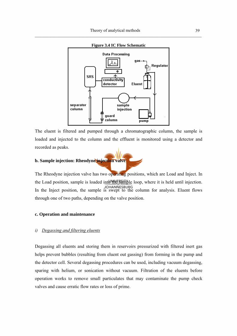
Theory of analytical methods ______________________________________________________________________________________
39
Figure 3.4 IC Flow Schematic
The eluent is filtered and pumped through a chromatographic column, the sample is
loaded and injected to the column and the effluent is monitored using a detector and
recorded as peaks.
b. Sample injection: Rheodyne injection valve
The Rheodyne injection valve has two operating positions, which are Load and Inject. In
the Load position, sample is loaded into the sample loop, where it is held until injection.
In the Inject position, the sample is swept to the column for analysis. Eluent flows
through one of two paths, depending on the valve position.
c. Operation and maintenance
i) Degassing and filtering eluents
Degassing all eluents and storing them in reservoirs pressurized with filtered inert gas
helps prevent bubbles (resulting from eluent out gassing) from forming in the pump and
the detector cell. Several degassing procedures can be used, including vacuum degassing,
sparing with helium, or sonication without vacuum. Filtration of the eluents before
operation works to remove small particulates that may contaminate the pump check
valves and cause erratic flow rates or loss of prime.
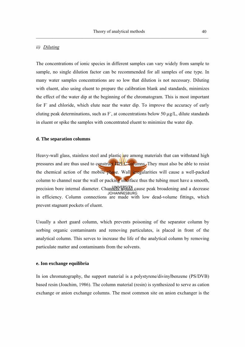
Theory of analytical methods ______________________________________________________________________________________
40
ii) Diluting
The concentrations of ionic species in different samples can vary widely from sample to
sample, no single dilution factor can be recommended for all samples of one type. In
many water samples concentrations are so low that dilution is not necessary. Diluting
with eluent, also using eluent to prepare the calibration blank and standards, minimizes
the effect of the water dip at the beginning of the chromatogram. This is most important
for F- and chloride, which elute near the water dip. To improve the accuracy of early
eluting peak determinations, such as F-, at concentrations below 50 µg/L, dilute standards
in eluent or spike the samples with concentrated eluent to minimize the water dip.
d. The separation columns
Heavy-wall glass, stainless steel and plastic are among materials that can withstand high
pressures and are thus used to construct HPLC columns. They must also be able to resist
the chemical action of the mobile phase. Wall irregularities will cause a well-packed
column to channel near the wall or packing interface thus the tubing must have a smooth,
precision bore internal diameter. Channels would cause peak broadening and a decrease
in efficiency. Column connections are made with low dead-volume fittings, which
prevent stagnant pockets of eluent.
Usually a short guard column, which prevents poisoning of the separator column by
sorbing organic contaminants and removing particulates, is placed in front of the
analytical column. This serves to increase the life of the analytical column by removing
particulate matter and contaminants from the solvents.
e. Ion exchange equilibria In ion chromatography, the support material is a polystyrene/divinylbenzene (PS/DVB)
based resin (Joachim, 1986). The column material (resin) is synthesized to serve as cation
exchange or anion exchange columns. The most common site on anion exchanger is the

Theory of analytical methods ______________________________________________________________________________________
41
tertiary amine group –N(CH3)3+OH-, a strong base and the sulphonic acid group –SO3
-H+
for a cation.
i) Anion-exchange resin
The anion-exchange resins used by Dionex are composed of a surface sulphonated
PS/DVB core (10-25 µm) and a totally porous latex particle which is completely
aminated. The latex particles have a considerably smaller diameter of about 0.1 µm and
carry the actual ion exchange function –NR3+. The structure of the anion exchange resins
used by Dionex and developed by Small is illustrated in Figure 3.5.
Figure 3.5 The structure of the anion exchange resins
The exchange process of a solution, which contains an anion, AX- on an anion exchange
column, is described by the following reaction.
xN(CH3)3+OH-(solid)+AX-(solution)↔(N(CH3)3
+)xAX-(solid)+xOH-(solution) (3.18)
The affinity of the resin for the anion relative to OH- ion is SO42->C2O4
2->I->NO3->Br-
>Cl->HCO2->OH->F-. These conditions depend on various factors, such as the type of
resin, size or the hydrated ion, and so on.
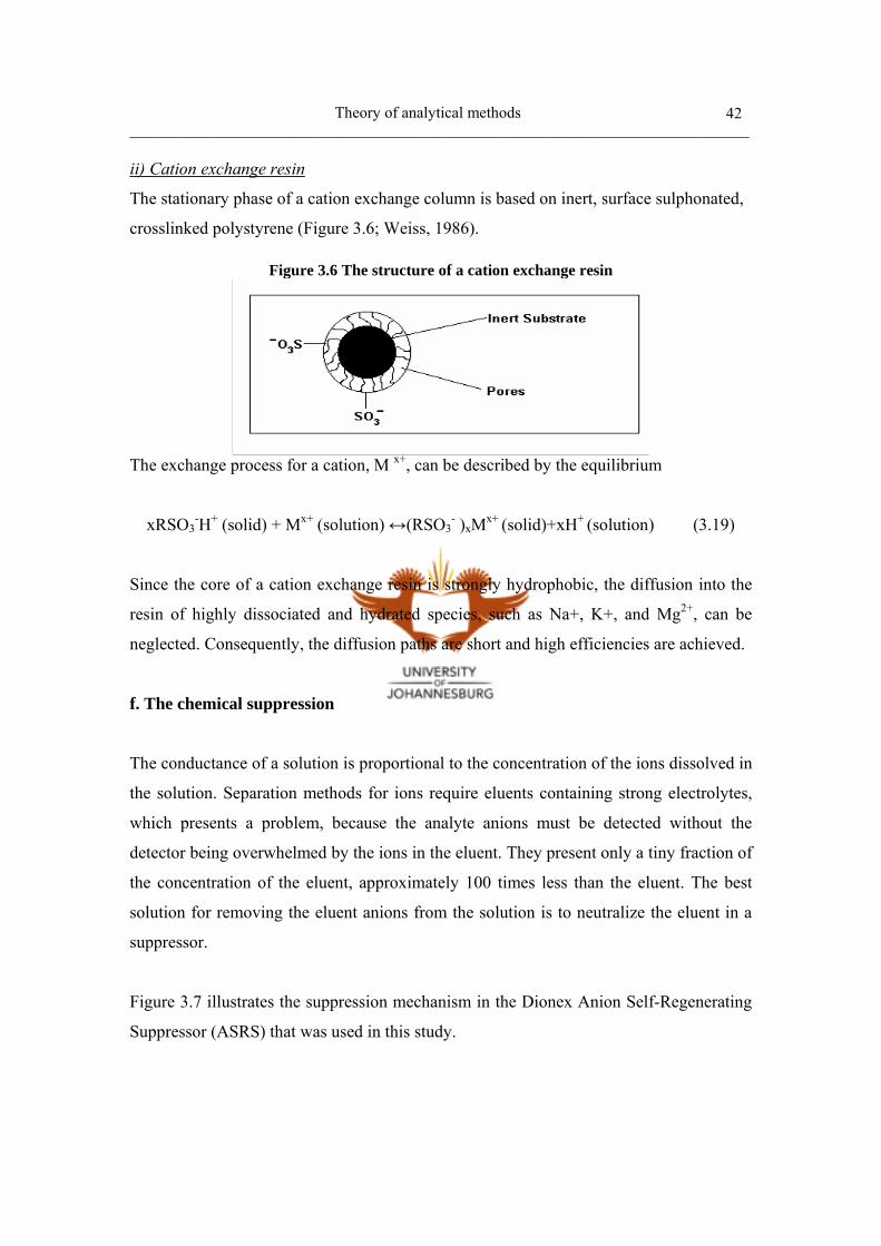
Theory of analytical methods ______________________________________________________________________________________
42
ii) Cation exchange resin
The stationary phase of a cation exchange column is based on inert, surface sulphonated,
crosslinked polystyrene (Figure 3.6; Weiss, 1986).
Figure 3.6 The structure of a cation exchange resin
The exchange process for a cation, M x+, can be described by the equilibrium
xRSO3-H+ (solid) + Mx+ (solution) ↔(RSO3
- )xMx+ (solid)+xH+ (solution) (3.19)
Since the core of a cation exchange resin is strongly hydrophobic, the diffusion into the
resin of highly dissociated and hydrated species, such as Na+, K+, and Mg2+, can be
neglected. Consequently, the diffusion paths are short and high efficiencies are achieved.
f. The chemical suppression
The conductance of a solution is proportional to the concentration of the ions dissolved in
the solution. Separation methods for ions require eluents containing strong electrolytes,
which presents a problem, because the analyte anions must be detected without the
detector being overwhelmed by the ions in the eluent. They present only a tiny fraction of
the concentration of the eluent, approximately 100 times less than the eluent. The best
solution for removing the eluent anions from the solution is to neutralize the eluent in a
suppressor.
Figure 3.7 illustrates the suppression mechanism in the Dionex Anion Self-Regenerating
Suppressor (ASRS) that was used in this study.
Theory of analytical methods ______________________________________________________________________________________
43
Figure 3.7 ASRS suppression mechanism
Analyte anions elute from the column with sodium counter ions. Two electrodes, one
beside each membrane (on the side opposite the eluent) hydrolyzes water to hydrogen
and hydroxide ions. Hydrogen ions diffuse across the membrane next to the anode,
neutralizing the eluent hydroxide to water, while sodium ions from the eluent diffuse
across the other membrane, providing counter ions to the hydroxide being generated at
the cathode.
In effect, sodium hydroxide from the eluent is transferred across the membrane and does
not reach the detector. The resulting eluent background conductivity is near zero,
considerably lower than before suppression. Also, the counter ion to the anion analytes is
now a hydrogen ion with conductivity seven times higher than the original sodium
counter ion. Since both the anion analyte and the cation counter ion produce the detector
response, response is increased. The suppressor lowers the background conductivity (and
thus the baseline noise and drift) and increases the signal. Suppression can also be
accomplished without water electrolysis by pumping a dilute sulfuric acid solution (the
regenerant) through the suppressor on the side of the membranes opposite the eluent.
For ion chromatography of cations, the suppressor membranes are anion exchange
polymers that allow anions to pass freely but exclude cations. The eluent uses dilute acids
such as methanesulfonic acid. In the Dionex Cation Self-Regenerating Suppressor
(CSRS), methanesulfonate counter ions are replaced by hydroxide generated by the

Theory of analytical methods ______________________________________________________________________________________
44
electrolysis of water. This neutralizes the acidic eluent and provides the highly
conductive hydroxide counter ion to the analyte cations.
g. Conductivity detection
Conductivity detectors are commonly used in ion chromatography mainly because of
their excellent sensitivity and predictable response to concentration changes. Ions in
solution conduct electrical current when a voltage is applied between electrodes in
contact with the solution. Since the magnitude of this current is proportional to the
concentration of dissolved ions, conductivity detection is useful for quantifying ionic
analytes.
i) Principle
The conductivity of a solution is measured by applying an alternating voltage between
two electrodes in a conductivity cell. At any instant in time, negatively charged anions
migrate toward the positive electrode and positively charged cations migrate toward the
negative electrode. Since the detector applies a known voltage to the cell electrodes and
the current is measured, the solution resistance, R, is calculated from Ohm’s law.
R = iE (3.20)
The inverse of the measured solution resistance is the conductance, G, measured in siemens (S).
G = R1 =
Ei (3.21)
The conductivity cell constant, K, corrects the measured conductance. The conductivity
of the solution is the conductance, which would be measured in a standard cell containing
electrodes of 1 cm2 surface area held 1 cm apart. This quantity is the conductivity, κ. The
units of conductivity are siemens per cm (S/cm).
K Gκ = × (3.22)

Theory of analytical methods ______________________________________________________________________________________
45
According to Kohlraush’s law of independent migration, conductivity is directly
proportional to concentration (that is, the conductivity of a dilute solution is the sum of
the individual contributions to conductivity of all the ions in the solution multiplied by
their concentration). Kohlraush’s law further states that each ion carries its portion of the
total conductivity without being affected by any of the other ions in solution. It is stated
as an equation:
К = 1000
∑ °
iiicλ (3.23)
Where: К = measured conductivity(S/cm), ci = concentration of the ions in equivalents/L (Equivalents/L equals moles/L times the charge on the ion)
The ionic limiting equivalent conductivity ( °iλ ) is specific for each ion. The unit for °
iλ is
S.cm2/equivalent. It is the conductivity of the ion divided by the concentration and
extrapolated to infinite dilution. Limiting equivalent conductivities for a number of
organic and inorganic ions are given in Table 3.2.
Table 3.2 Limiting equivalent conductivities at 25 ° C Anions °
iλ Cations °iλ
OH- 198 H+ 350
F- 54 Li+ 39
Cl- 76 Na+ 50
Br- 78 K+ 74
I- 77 NH4+ 73
NO3- 71 Mg2+ 53
HCO3- 45 Ca2+ 60
SO42- 80 Sr2+ 59
Acetate 41 CH3NH3+ 58
Benzoate 32 N(CH3CH2)4+ 33
Values of °iλ from Table 3.2 can be used to calculate conductivities of solutions
containing ions. For example, the limiting equivalent conductivity for NaCl at 25 ºC is
126.5. This is the sum of the ionic limiting equivalent conductivity for Na+, which is 50.1,
plus that of Cl-, which are 76.4. A 0.1 mM solution of NaCl at 25 ºC has a conductivity of
0.1×126.5, or 12.65 µS/cm.
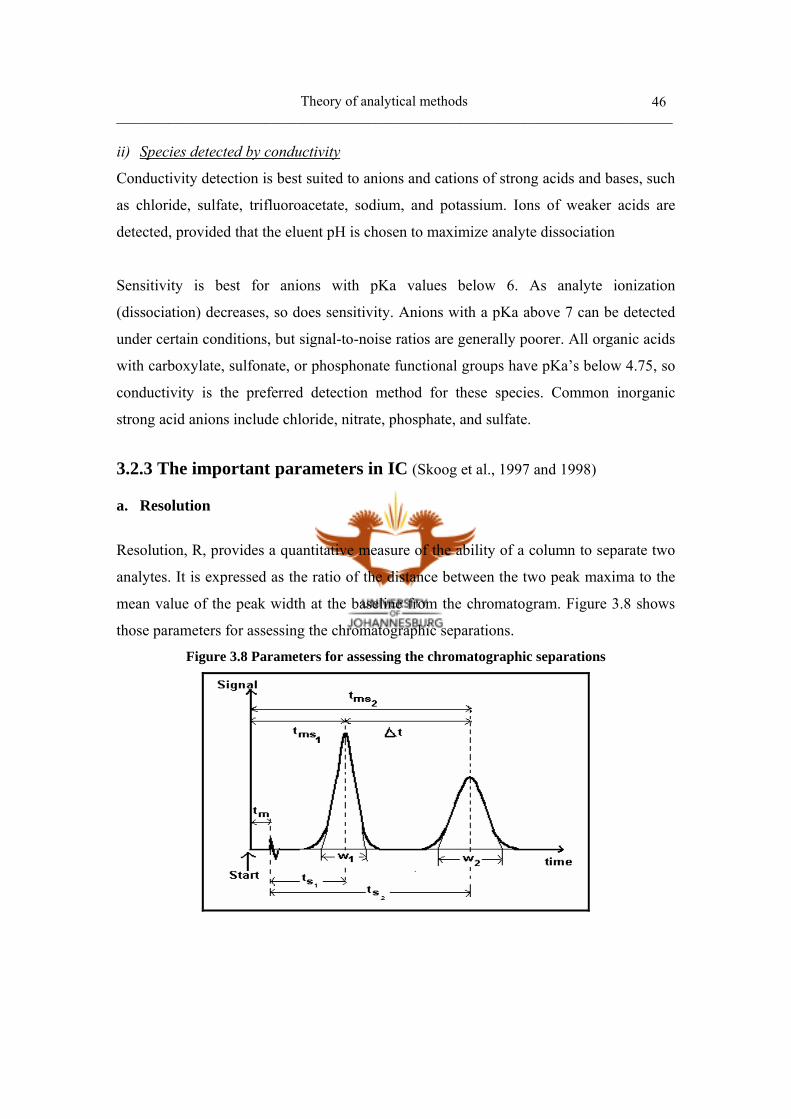
Theory of analytical methods ______________________________________________________________________________________
46
ii) Species detected by conductivity
Conductivity detection is best suited to anions and cations of strong acids and bases, such
as chloride, sulfate, trifluoroacetate, sodium, and potassium. Ions of weaker acids are
detected, provided that the eluent pH is chosen to maximize analyte dissociation
Sensitivity is best for anions with pKa values below 6. As analyte ionization
(dissociation) decreases, so does sensitivity. Anions with a pKa above 7 can be detected
under certain conditions, but signal-to-noise ratios are generally poorer. All organic acids
with carboxylate, sulfonate, or phosphonate functional groups have pKa’s below 4.75, so
conductivity is the preferred detection method for these species. Common inorganic
strong acid anions include chloride, nitrate, phosphate, and sulfate.
3.2.3 The important parameters in IC (Skoog et al., 1997 and 1998) a. Resolution
Resolution, R, provides a quantitative measure of the ability of a column to separate two
analytes. It is expressed as the ratio of the distance between the two peak maxima to the
mean value of the peak width at the baseline from the chromatogram. Figure 3.8 shows
those parameters for assessing the chromatographic separations.
Figure 3.8 Parameters for assessing the chromatographic separations

Theory of analytical methods ______________________________________________________________________________________
47
The equation of the resolution is given below.
R =
221
12
wwtt msms
+− =
21
2wwt
+∆ (3.24)
Where, tms2 and tms1: Gross retention times for peaks 1 and 2 respectively w1 and w2: Peak widths along the baseline of peak 1 and 2 respectively
The resolution should be at least 0.5 to confirm two peaks as separate peaks and if R is
greater than 1.5 two peaks are considered as completely separate peaks. The resolution
can be improved by lengthening the column but this will also increase the analysis time.
i) Capacity factor (k’)
Capacity factor is a dimensionless measure of retention, which is independent of column
length or eluent flow rate. It is calculated as follows:
k’ = m
ms
ttt − (3.25)
Where: ts = retention time of solute tm = retention time of unretained solute (column void volume)
Small values of k’ imply that the compound elutes near the void volume. Thus, the
separation will be very poor. Large k’ values indicate a good separation but also imply
longer analysis times, an associated peak broadening, and a decrease in sensitivity.
ii) Column efficiency (N) (theoretical plates)
It is a measure of the narrowness of analyte bands as they elute from the column. High
efficiency is desirable because resolution between closely spaced bands improves with
greater efficiency. For a symmetrical (Gaussian) peak, column efficiency can be
determined by the following:
N = 5.54 2
2/1
1⎟⎟⎠
⎞⎜⎜⎝
⎛W
t (3.26)
Where: t1 = the peak retention time, in seconds W1/2 = the peak width at 1/2 height, in seconds
Theory of analytical methods ______________________________________________________________________________________
48
Column efficiency is proportional to column length, for a given resin and column
diameter, increasing the column length increases the column efficiency.
3.3 Inductively Coupled Plasma-Optical Emission Spectroscopy (ICP-OES)
3.3.1 Introduction Plasma is a partly ionized gas (often argon), which contains particles of various types
such as electrons, atoms, ions and molecules, maintained by an external field. As a whole,
it is electrically neutral. The most common plasma source is the ICP torch (Lajunen,
1991). The introduction of ICP as a source for analytical atomic emission spectrometry
constituted a revolutionary advance in that field. The performance characteristics of ICP-
OES, specifically its versatility, wide applicability, and ease of use, were almost
unparalleled among methods of elemental analysis.
ICP-OES is a major technique for quantitative multi-element analysis and very powerful
analytical tool. In terms of sensitivity, ICP-OES is generally comparable to flame atomic
absorption, i.e. detection limits are typically at the µg/L level in aqueous solutions
(Varma, 1991).
3.3.2 Instrumentation for ICP-OES (Lajunen , 1991; Varma, 1991; Liberty, 1991) A typical arrangement for ICP-OES is shown in Figure 3.9 and consists of a sample
introduction system, the ICP torch and its associated gas supplies, a radio-frequency
generator, an optical spectrometer, detectors and associated electronics and computerized
instrument control, data collection and analysis.

Theory of analytical methods ______________________________________________________________________________________
49
Figure 3.9 ICP instrumentation (http://icp-oes.com/instrument_layout.htm, Moore, 1989)
a. Sample introduction
For most analysis the liquid sample is pumped into a pneumatic nebuliser (Figure3.9),
which aspirates the sample with high velocity argon, forming a fine aerosol. The aerosol
then passes into a spray chamber where larger droplets are removed via a drain (Jarvis et
al., 1992). Typically, only 2% of the original aerosol passes through the spray chamber
(Olesik, 1996). This process is necessary to produce droplets small enough to be
vaporized in the plasma torch. The finer droplets in the vapor are transported to the
plasma.
b. ICP torch It is formed when energy is transferred to a gas, usually argon, by means of an induction
coil. The plasma forms above the inner tube (Plasma tube) and within the outer tube
(coolant tube) and its location are largely determined by the position of the induction coil
(Figure 3.10).

Theory of analytical methods ______________________________________________________________________________________
50
Figure 3.10 Inductively coupled plasma (Moore, 1989)
i) The formation mechanism of the ICP
The induction coil, which is part of an oscillator circuit, commonly a radio frequency
generator, induces a strong high-frequency magnetic field. The magnetic field, generated
by the RF-currents, induces an electric field in the coil region. When seed electrons and
ions, formed by the generation of a spark in the argon stream using a Tesla coil, are
introduced, the electrons accelerate and encounter resistance through collisions with
argon atoms. This collision yields an avalanche of charged particles in sufficient numbers
to absorb the energy from the radio frequency field. Once the electrons reach the
ionization potential of the plasma support gas (usually argon), further ionization takes
place, and stable self-sustaining plasma is formed. A vortex flow of argon is used to cool
the inside walls of the torch for protecting the outer tube from the very hot plasma (6000
to 10000 K) and stabilizes and thermally isolates the plasma.
ii) Zones in the ICP
The various processes occurring in the ICP lead to several rather distinct zones, with very
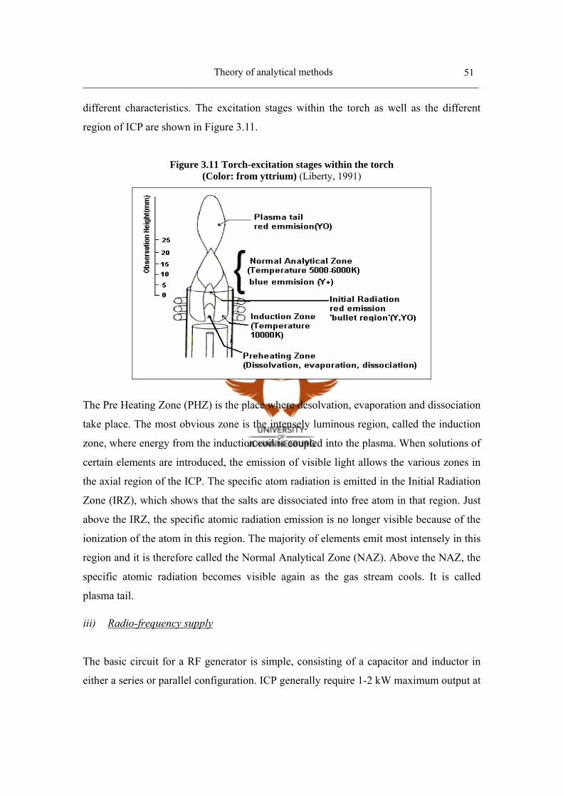
Theory of analytical methods ______________________________________________________________________________________
51
different characteristics. The excitation stages within the torch as well as the different
region of ICP are shown in Figure 3.11.
Figure 3.11 Torch-excitation stages within the torch (Color: from yttrium) (Liberty, 1991)
The Pre Heating Zone (PHZ) is the place where desolvation, evaporation and dissociation
take place. The most obvious zone is the intensely luminous region, called the induction
zone, where energy from the induction coil is coupled into the plasma. When solutions of
certain elements are introduced, the emission of visible light allows the various zones in
the axial region of the ICP. The specific atom radiation is emitted in the Initial Radiation
Zone (IRZ), which shows that the salts are dissociated into free atom in that region. Just
above the IRZ, the specific atomic radiation emission is no longer visible because of the
ionization of the atom in this region. The majority of elements emit most intensely in this
region and it is therefore called the Normal Analytical Zone (NAZ). Above the NAZ, the
specific atomic radiation becomes visible again as the gas stream cools. It is called
plasma tail.
iii) Radio-frequency supply
The basic circuit for a RF generator is simple, consisting of a capacitor and inductor in
either a series or parallel configuration. ICP generally require 1-2 kW maximum output at
Theory of analytical methods ______________________________________________________________________________________
52
Radio Frequency (RF) to maintain the plasma. The RF generator in the Varian ICP-OES
instrument is based on a 40.68 MHz crystal-controlled oscillator and has automatic
tuning and automatic level control and is rated at 1.7 kW.
iv) Optical spectrometer
A spectrometer consists of three main parts: An emission source, which produces the
spectrum, an optical system, which scatters the spectrum and the device to measure the
emitted lines that processes the result. A common spectrometer optical system consists of
a polychromator or a monochromator, which scatters the spectrum and isolates the
analytical lines of the elements to be analyzed.
v) Detectors and readout systems
In optical emission spectrometry, photo-multipliers are commonly used as detectors.
They are photocell detectors. The incident photons coming from the exit slit liberate
electrons from the photo cathode and the electron flow is then amplified by a set of
dynodes. The final anode current is proportional to the incident photon signal received by
the photo cathode. The measurement dynamic range is very broad, i.e. 1015, and
sensitivity is high, as the dark current is low. These detectors allow the detection of low
intensities emitted by trace elements, as well as strong signals from major elements. They
have very fast response times, typically 1-2 ns for a 10%-90% change in signal. A fatigue
lamp (a small incandescent light source) is often used with photo-multipliers to keep the
temperature of the tube and its associated electronics constant. The fatigue lamp is
switched on when the emission source is off and switched off when the emission source
is on.
3.3.3 ICP process (Liberty p10)
The sample being analysed is introduced into the plasma as a fine droplet aerosol. The
processes, which occur while the aerosol moves up through the plasma, are described in
Figure 3.12.
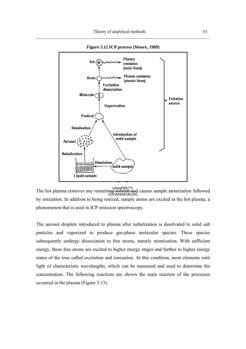
Theory of analytical methods ______________________________________________________________________________________
53
Figure 3.12 ICP process (Moore, 1989)
The hot plasma removes any remaining solvent and causes sample atomization followed
by ionization. In addition to being ionized, sample atoms are excited in the hot plasma, a
phenomenon that is used in ICP emission spectroscopy.
The aerosol droplets introduced to plasma after nebulization is desolvated to solid salt
particles and vaporized to produce gas-phase molecular species. These species
subsequently undergo dissociation to free atoms, namely atomization. With sufficient
energy, these free atoms are excited to higher energy stages and further to higher energy
states of the ions called excitation and ionization. At this condition, most elements emit
light of characteristic wavelengths, which can be measured and used to determine the
concentration. The following reactions are shown the main reaction of the processes
occurred in the plasma (Figure 3.13).
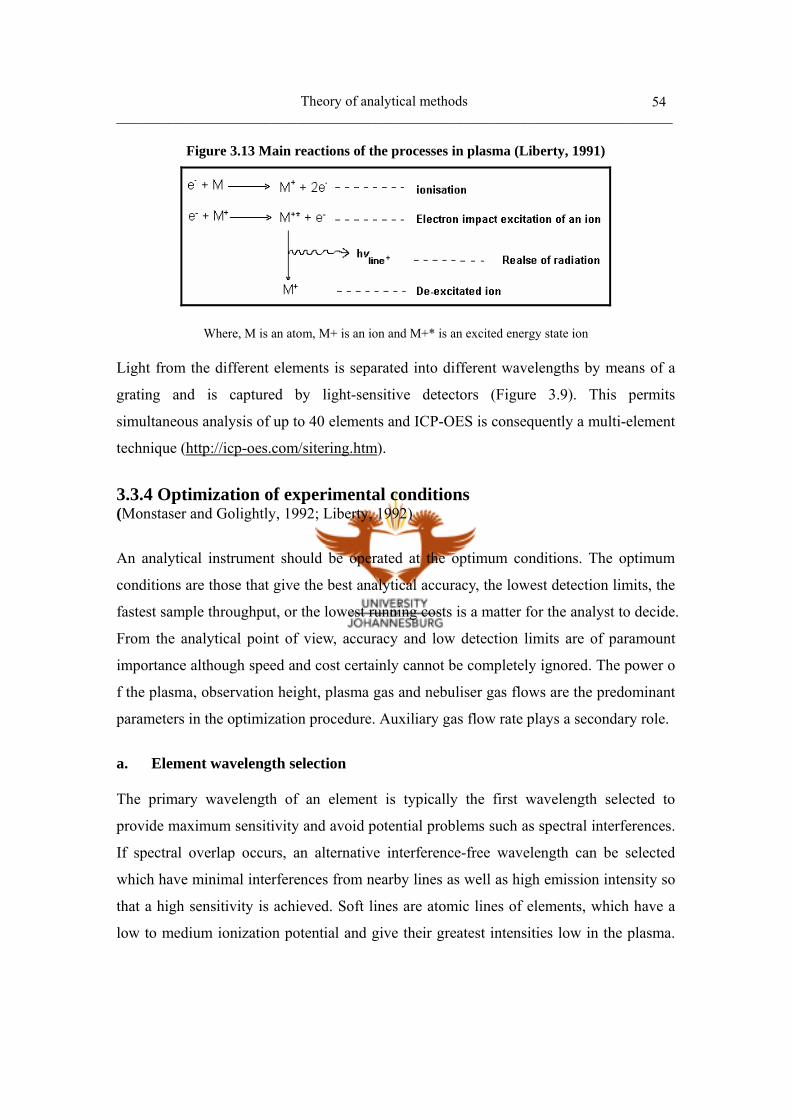
Theory of analytical methods ______________________________________________________________________________________
54
Figure 3.13 Main reactions of the processes in plasma (Liberty, 1991)
Where, M is an atom, M+ is an ion and M+* is an excited energy state ion
Light from the different elements is separated into different wavelengths by means of a
grating and is captured by light-sensitive detectors (Figure 3.9). This permits
simultaneous analysis of up to 40 elements and ICP-OES is consequently a multi-element
technique (http://icp-oes.com/sitering.htm).
3.3.4 Optimization of experimental conditions (Monstaser and Golightly, 1992; Liberty, 1992)
An analytical instrument should be operated at the optimum conditions. The optimum
conditions are those that give the best analytical accuracy, the lowest detection limits, the
fastest sample throughput, or the lowest running costs is a matter for the analyst to decide.
From the analytical point of view, accuracy and low detection limits are of paramount
importance although speed and cost certainly cannot be completely ignored. The power o
f the plasma, observation height, plasma gas and nebuliser gas flows are the predominant
parameters in the optimization procedure. Auxiliary gas flow rate plays a secondary role.
a. Element wavelength selection The primary wavelength of an element is typically the first wavelength selected to
provide maximum sensitivity and avoid potential problems such as spectral interferences.
If spectral overlap occurs, an alternative interference-free wavelength can be selected
which have minimal interferences from nearby lines as well as high emission intensity so
that a high sensitivity is achieved. Soft lines are atomic lines of elements, which have a
low to medium ionization potential and give their greatest intensities low in the plasma.
Theory of analytical methods ______________________________________________________________________________________
55
Hard lines are atomic or ionic lines, which have greater excitation potentials and their
greatest intensity occurs characteristically at greater observation heights in the plasma.
b. Plasma observation height The intensity of the emission at individual wavelengths varies according to the region in
the plasma that is observed. Observation height is a critical parameter that can
significantly enhance sensitivity. When analyzing high concentration levels it is best to
optimize by intensity, as the background signal will be insignificant when compared to
the large analyte signal. Optimization by signal to background ratio should be used when
analyzing low concentration levels as the background signal becomes significant.
c. Plasma power The plasma power is another critical parameter that can significantly enhance the signal
of selected wavelengths. Higher power settings increase the intensity of hard wavelength.
However, the background is also enhanced at higher power settings. The extent to which
the background is raised depends on the wavelength. Thus it is important to monitor the
effect of increased power settings on background as the increase in gross analyte signal
may be caused by an increase in background levels and not net analyte signal. The
intensity of soft lines on the other hand, generally do not increase significantly with
higher powers because they correspond to low energy transitions and therefore are
already near their maximum sensitivity at lower powers.
d. Plasma gas flow rate
Increasing the plasma gas increases the size of the hot, analytical zone within the plasma.
Thus the intensity of hard wavelengths increases with high plasma gas flow rates as
higher energy transitions can occur due to an increase in available energy.
e. Auxiliary gas flow rate
The main effect of the auxiliary gas is to lift the plasma away from the torch. Higher
auxiliary gas flows can reduce band structures.

Theory of analytical methods ______________________________________________________________________________________
56
f. Nebuliser pressure
The intensity of hard wavelengths increased significantly by intensity reducing the
nebuliser pressure. This occurs because the reduced pressure allows an increase in the
residence time of the analyte in the plasma. Thus the analyte is given a longer time to
acquire the energy for high-energy transitions. However, when the nebuliser pressure is
too low instability occurs in the nebuliser operation.
3.4 Inductively Coupled Plasma Mass Spectroscopy (ICP-MS) 3.4.1 Introduction Inductively Coupled Plasma Mass Spectrometry (ICP-MS) is a very powerful tool for
trace elemental analysis. It was developed in the 1980’s and has grown rapidly to be one
of the most important techniques for elemental analysis because of the following benefits:
(Houk, 1986; Monstaser, 1992; Vela et al., 1993)
• A very low detection limit (ng/L-mg/L)
• A very simple and unique mass spectrum of the elements
• The ability to measure elemental isotope ratios
• A good precision and accuracy
• Multielement determination
ICP-MS has been used widely over the years, finding applications in a number of
different fields including drinking water, wastewater, natural water
systems/hydrogeology, geology and soil science, mining/metallurgy, food sciences, and
medicine. 3.4.2 Instrumentation and process of the ICP-MS
In principle, the ICP-MS technology is very similar to the ICP-OES with regard to the
process that samples are decomposed to neutral elements in high temperature argon
plasma. However, unlike ICP-OES, ICP-MS accomplished the elemental determination
by counting the number of ions at a certain mass of the element instead of the light

Theory of analytical methods ______________________________________________________________________________________
57
emitted by the element. The interface system is of unique importance in ICP-MS and this
subject is treated extensively in this section.
An ICP-MS can be thought of as four main processes, including sample introduction and
aerosol generation, ionization by an argon plasma source, mass discrimination, and the
detection system. Since the first two processes were already discussed in Section 3.3.2.a
and 3.3.2.b. The mass discrimination and the detection system are considered here. The
schematic below illustrates this sequence of processes.
Figure 3.14 Schematic of an ICP-MS system (Skoog et al. 1998)
a. Mass discrimination
i) ICP-MS interface-sampling ions
The entire mass spectrometer must be kept in a vacuum so that the ions are free to move
without collisions with air molecules. Since atomization/ionization occurs at atmospheric
pressure, a pumping system is needed to continuously pull a vacuum inside the
spectrometer. The Figure 3.15 shows the Mass Spectroscopy interface.
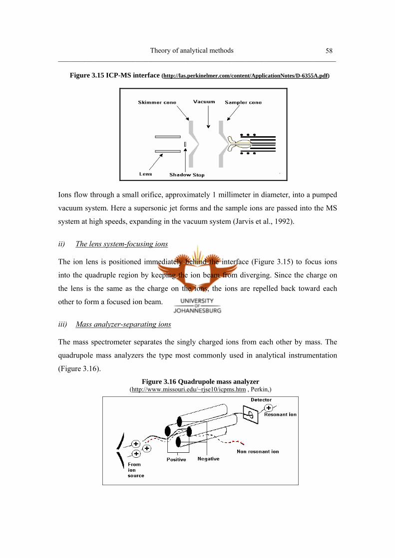
Theory of analytical methods ______________________________________________________________________________________
58
Figure 3.15 ICP-MS interface (http://las.perkinelmer.com/content/ApplicationNotes/D-6355A.pdf)
Ions flow through a small orifice, approximately 1 millimeter in diameter, into a pumped
vacuum system. Here a supersonic jet forms and the sample ions are passed into the MS
system at high speeds, expanding in the vacuum system (Jarvis et al., 1992).
ii) The lens system-focusing ions
The ion lens is positioned immediately behind the interface (Figure 3.15) to focus ions
into the quadruple region by keeping the ion beam from diverging. Since the charge on
the lens is the same as the charge on the ions, the ions are repelled back toward each
other to form a focused ion beam.
iii) Mass analyzer-separating ions
The mass spectrometer separates the singly charged ions from each other by mass. The
quadrupole mass analyzers the type most commonly used in analytical instrumentation
(Figure 3.16).
Figure 3.16 Quadrupole mass analyzer (http://www.missouri.edu/~rjse10/icpms.htm , Perkin,)

Theory of analytical methods ______________________________________________________________________________________
59
It is made up of four metal rods aligned in a parallel diamond pattern. A combined DC
and AC electrical potential is applied to the rods with opposite rods having a net negative
or positive potential. Ions enter into the path between all of the rods. When the DC and
AC voltages are set to certain values only one particular ion is able to continue on a path
between the rods and the others, which are unstable at this voltage combination, are
forced out of this path. This ion will have a specific mass-to-charge (m/z) ratio. Many
combinations of voltages are chosen which allows an array of different m/z ratio ions to
be detected.
b. Detection system – counting ions
Ions leaving the quadrupole strike the active surface of the detector, known as a dynode,
and generate a measurable electronic signal. The detection system operates on the
principle of electron multiplication. The drawing below is an ICP-MS detector.
Figure 3.17 ICP-MS detector
An ion striking the first dynode releases electrons, which accelerate towards and into the
dynode beneath which in turn releases, more electrons. This cascading of electrons
continues until a measurable pulse is created. By counting the pulses generated by the
detector, the system counts the ions that hit the first dynode.
Evaluation of instrumental methods for low-level F- determination in laboratory test samples ______________________________________________________________________________________
60
Chapter 4
Evaluation of instrumental methods for low-level Fluoride (F-) determination in laboratory test samples
4.1 Objective
Fluoride (F-) in water can be determined in a number of ways, using instrumental
methods such as potentiometry with Ion-Selective Electrodes (ISE) (Richard 1969;
Cardwell et al., 1994; Wang, 1995; McCaffrey, 1994; Lopes da Conceição, 2000; van
Staden, 2000; US EPA method 13B), spectrophotometry (Bellack 1958; Crosby et al.,
1968; Cabello-Tomas and west, 1969; Wada et al. 1985; Yuchi et al., 1995; Khalifa and
Hafez, 1998; Oszwaldowski et al., 1998; Faraj-Zadeh and Kalhor, 2001; Nishimoto et al.,
2001; Garrido et al., 2002; Arancibia et al., 2004; US EPA method 13A), inductively
coupled plasma-mass spectrometry (Bayón et al., 1999; Okamoto, 2001), capillary
conductometry (Buffle et al., 1985), complexometry (Pickering, 1986; Saha, 1993), gas
diffusion (Cardwell et al., 1994), capillary ion analysis (Bondoux and Jones, 1995; Saad
et al., 1998), and ion chromatography (IC) (Jones, 1992; McCarthy, 1994; Hirayama et al.,
1996; Moskvin et al., 1998; Jackson et al., 2000; Jackson, 2001; Application note
133,135,140 and 154).
For the determination of F-, F- Ion Selective Electrode (F-ISE) has been widely used due
to its simplicity and short analysis time. The Ion Chromatography (IC) technique has also
come into prominence in terms of selectivity and sensitivity. Although the SPANDS
method achieved very high sensitivity, this method was displaced by the ISE due to its
main disadvantages; poor selectivity, labour-intensiveness and being time consuming due
to the distillation step (Crosby et al., 1968; Mac Leod and Crist, 1973; Oszwaldowski et
al., 1998). This method was not included in this comparative study. F-ISE and IC
methods have been used for achieving the objectives given in Chapter 1.
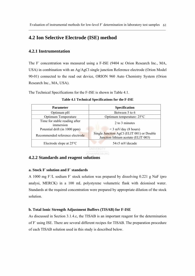
Evaluation of instrumental methods for low-level F- determination in laboratory test samples ______________________________________________________________________________________
61
4.2 Ion Selective Electrode (ISE) method 4.2.1 Instrumentation
The F- concentration was measured using a F-ISE (9404 sc Orion Research Inc., MA,
USA) in combination with an Ag/AgCl single junction Reference electrode (Orion Model
90-01) connected to the read out device, ORION 960 Auto Chemistry System (Orion
Research Inc., MA, USA).
The Technical Specifications for the F-ISE is shown in Table 4.1.
Table 4.1 Technical Specifications for the F-ISE
Parameter Specification Optimum pH Between 5 to 6
Optimum Temperature Optimum temperature: 25°C Time for stable reading after
immersion 2 to 3 minutes
Potential drift (in 1000 ppm) < 3 mV/day (8 hours)
Recommended reference electrode Single Junction AgCl (ELIT 001) or Double Junction lithium acetate (ELIT 003)
Electrode slope at 25°C 54±5 mV/decade
4.2.2 Standards and reagent solutions
a. Stock F- solution and F- standards
A 1000 mg F-/L sodium F- stock solution was prepared by dissolving 0.221 g NaF (pro
analysi, MERCK) in a 100 mL polystyrene volumetric flask with deionised water.
Standards at the required concentration were prepared by appropriate dilution of the stock
solution.
b. Total Ionic Strength Adjustment Buffers (TISAB) for F-ISE
As discussed in Section 3.1.4.c, the TISAB is an important reagent for the determination
of F- using ISE. There are several different recipes for TISAB. The preparation procedure
of each TISAB solution used in this study is described below.
Evaluation of instrumental methods for low-level F- determination in laboratory test samples ______________________________________________________________________________________
62
i) TISAB III
TISAB III is commercially available from Thermo Orion (Orion Research Inc., Beverly,
MA, USA, Cat. No.940911). It contains CDTA (trans-1,2-cyclohexylendinitrilo) tetra-
acetic acid) and ammonium acetate (CH3COONH4) buffer at pH 5.5. The recommended
volume ratio between TISAB and test solution was 1:10. 20 mL of test solution and 2 mL
of TISAB III mixed in a plastic beaker was used in this study.
ii) TISAB IV
It contains TRIS buffer for high levels of Al interference at pH 8.5. 84 mL concentrated
HCl (36-38%), 242g tris(hydroxymethyl)aminomethane, and 230 g sodium tartrate
(Na2C4H4O6 •2H2O), were added to 500 mL deionised water, allowed to dissolve, and
then made up to 1 L in a volumetric flask with deionised water. A recommended volume
ratio between TISAB and test solution, written in the manual (Orion, 1982) was 1:1. In
this study, 10 mL of test solution and 10 mL of TISAB IV mixed in a plastic beaker.
iii) Low Level TISAB (LLT)
This is used when measuring samples containing less than 0.4 mg/L F- and no F-
complexing agents, such as Fe or Al, are present. 57 mL acetic acid and 58 g sodium
chloride were added in 500 mL distilled water and the pH was adjusted to 5.5 by adding
drops of 5 M NaOH after cooling the solution, then made up to 1 L in a volumetric flask
with deionised water. The recommended volume ratio between TISAB and test solution
was 1:1. 10 mL of test solution and 10 mL of Low Level TISAB mixed in a plastic
beaker was used in this study.
4.2.3 Results and discussion
a. Electrode drift
One of the main problems in ISE measurement is the drift in electrode potential during a
sequence of measurements. 0.02, 0.1, 1, 2 mg/L spiked samples of F- in deionised water
were prepared in 100 mL polystyrene volumetric flasks. 20 mL of sample and 2 mL of
TISAB III were added into a 50 mL polystyrene beaker for measurement. The uncertainty,
due to fluctuating potential values during the first a few seconds after immersion of the

Evaluation of instrumental methods for low-level F- determination in laboratory test samples ______________________________________________________________________________________
63
electrode, was controlled by the following procedure. The reference electrode was placed
into the beaker first, followed after 3 minutes by the F- electrode. The potential was
recorded from 3 minutes after immersion of the F- electrode for 1 hour and drift values
were calculated by subtraction. These experiments were repeated 3 times for each sample.
The electrodes were rinsed by spraying with a jet of deionised water and gently dabbed
dry with a soft tissue before measurement.
A summary of results, which shows the average drift (mV/h) and standard deviation
obtained in this experiment, is given in Table 4.2.
Table 4.2 Potential Drift (mV) at each F- concentration vs. time
[F] Known 0.02 mg/L 0.1 mg/L 1 mg/L 2 mg/L Time (min) P*1 P2 P3 P1 P2 P3 P1 P2 P3 P1 P2 P3
3 154.6 153.4 159.4 139.5 138.2 138.8 90.4 90.6 89 73.7 73.9 74.25 154.5 153.4 159.4 139.4 139.1 138.7 90.3 90.5 88.9 73.7 73.9 74.17 154.5 153.3 159.4 139.2 139 138.6 90.2 90.4 - 73.7 73.8 74.1
10 154.7 153.3 159.0 139.1 138.9 138.5 90.2 90.4 - 73.7 73.7 74.115 154.8 153.3 158.8 139 138.8 138.4 90.2 90.3 88.7 73.7 73.6 74.030 154.6 153.4 158.3 138.6 138.5 138.2 90.1 90.2 88.4 73.6 73.3 73.860 153.7 152.5 157.5 137.9 138 137.8 89.4 89.6 87.9 73.1 73 73.5
Drift 1.1 0.9 1.9 1.6 1.1 1 1.0 1.0 1.1 0.6 0.9 0.7 Average
Drift (mV/h) 1.30 ± 0.53 1.23± 0.32 1.03± 0.06 0.73± 0.15
P* = Potential (mV)
These results show that the average drift values of the F- electrode are bigger when the
concentrations of F- are lower. This trend is evident in the standard deviations. The
standard deviations for the 0.02 and 0.1 mg/L solutions are larger than those for 1 and 2
mg/L F- solutions. This means that lower concentrations of F- are more severely
influenced by drift and show poor precision. Therefore, steps must be taken to minimize
the drift for the determination of F- at levels less than 1 mg/L. Further investigation was
done in order to determine the best procedure to minimize electrode drift and decrease
response time at the 0.02 to 1 mg/L F- concentration level.
b. Investigation of electrode response
The objective of this study was establishing the most effective way to minimize the
electrode drift. 0.02, 0.1 mg/L spiked samples of F- in deionised water were prepared
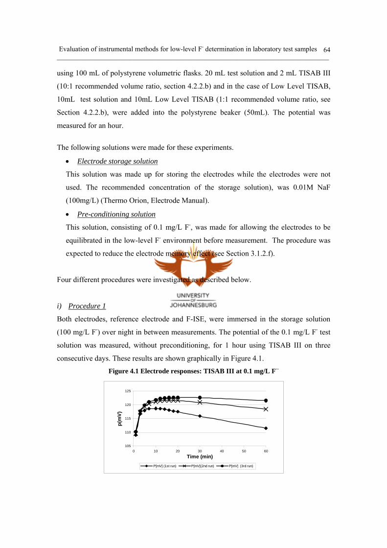
Evaluation of instrumental methods for low-level F- determination in laboratory test samples ______________________________________________________________________________________
64
using 100 mL of polystyrene volumetric flasks. 20 mL test solution and 2 mL TISAB III
(10:1 recommended volume ratio, section 4.2.2.b) and in the case of Low Level TISAB,
10mL test solution and 10mL Low Level TISAB (1:1 recommended volume ratio, see
Section 4.2.2.b), were added into the polystyrene beaker (50mL). The potential was
measured for an hour.
The following solutions were made for these experiments.
• Electrode storage solution
This solution was made up for storing the electrodes while the electrodes were not
used. The recommended concentration of the storage solution), was 0.01M NaF
(100mg/L) (Thermo Orion, Electrode Manual).
• Pre-conditioning solution
This solution, consisting of 0.1 mg/L F-, was made for allowing the electrodes to be
equilibrated in the low-level F- environment before measurement. The procedure was
expected to reduce the electrode memory effect (see Section 3.1.2.f).
Four different procedures were investigated as described below.
i) Procedure 1
Both electrodes, reference electrode and F-ISE, were immersed in the storage solution
(100 mg/L F-) over night in between measurements. The potential of the 0.1 mg/L F- test
solution was measured, without preconditioning, for 1 hour using TISAB III on three
consecutive days. These results are shown graphically in Figure 4.1.
Figure 4.1 Electrode responses: TISAB III at 0.1 mg/L F--
105
110
115
120
125
0 10 20 30 40 50 60
Time (min)
p(m
V)
P[mV] (1st run) P[mV](2nd run) P[mV] (3rd run)

Evaluation of instrumental methods for low-level F- determination in laboratory test samples ______________________________________________________________________________________
65
The drift in each run was quite different, although the same electrodes and solutions were
used. The first part of the graph, between 0 to 5 minutes shows a similar trend in each run.
In a subsequent experiment the intra-day electrode response was investigated. This is
discussed in the next paragraph.
ii) Procedure 2
Both electrodes (reference electrode and F-ISE) were immersed in the storage solution
(100 mg/L F-) over night. Before the first potential measurement of the test solutions, the
electrodes were put into the pre-conditioning solution (0.1 mg/L) for 20 minutes. The test
solution, 0.1 mg/L, was then measured for 1 hour using TISAB III the potential recorded.
After finishing the first measurement, the electrodes were immersed into the storage
solution again for 50 minutes to allow the electrodes to be equilibrated under similar
conditions as before (Procedure 1). The procedure was then repeated twice on the same
day. The results are summarized in Figure 4.2.
Figure 4.2 Electrode response: TISAB III at 0.1 mg/L F-
100
110
120
130
140
150
160
0 10 20 30 40 50 60
Time(min)
Pote
ntia
l(mV)
P1 P2 P3
This graph shows that the response during the same day is reproducible. Compared to the
Procedure 1 (Figure 4.1), procedure 2 yielded more reproducible results (Figure 4.2). The
response time to obtain a stable reading was, however, not improved as was expected
using a preconditioning solution.

Evaluation of instrumental methods for low-level F- determination in laboratory test samples ______________________________________________________________________________________
66
iii) Procedure 3
Preconditioning was used between every single measurement in Procedure 2, but this was
not so effective to reduce drift, as was expected. Thus, in Procedure 3, preconditioning
was used on the test solutions (0.02 mg/L and 0.1 mg/L) only for the first measurement in
a series. The results are given in Figure 4.3.
Figure 4.3 Electrode response: TISAB III at 0.02 mg/L and 0.1 mg/L F-
100
110
120
130
140
0 10 20 30 40 50 60Time(min)
Pote
ntia
l(mV)
P1(0.1mg/l) P2(0.1mg/l) P3(0.1mg/l)P1(0.02mg/l) P2(0.02mg/l) P3(0.02mg/l)
Each graph of the first run displays a longer equilibration time and a bigger change of
potential. This means that the electrode takes a long time to adjust after exposure to high
F- concentrations. The potential of the first run varied from low to high value, while the
potential of the second and the third run varied from high to low value. This was because
the electrode was not exposed to high concentration of the storage solution between
measurements. After the first measurement, the electrodes were rinsed by spraying with a
jet of deionised water, which did not contain any F-. The initial high potential values in
the second run were caused by the exposure of the ion selective membrane to the non-F-
environment of deionised water.
iv) Procedure 4
F- electrode become sluggish over time. Brushing the membrane with F- toothpaste can
restore the performance of the electrodes (Thermo Orion, Application note). This
experiment was done after F-ISE had been used for 8 months and 3 months after the
experiment of Procedure 2.
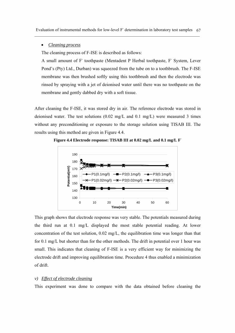
Evaluation of instrumental methods for low-level F- determination in laboratory test samples ______________________________________________________________________________________
67
• Cleaning process
The cleaning process of F-ISE is described as follows:
A small amount of F- toothpaste (Mentadent P Herbal toothpaste, F- System, Lever
Pond’s (Pty) Ltd., Durban) was squeezed from the tube on to a toothbrush. The F-ISE
membrane was then brushed softly using this toothbrush and then the electrode was
rinsed by spraying with a jet of deionised water until there was no toothpaste on the
membrane and gently dabbed dry with a soft tissue.
After cleaning the F-ISE, it was stored dry in air. The reference electrode was stored in
deionised water. The test solutions (0.02 mg/L and 0.1 mg/L) were measured 3 times
without any preconditioning or exposure to the storage solution using TISAB III. The
results using this method are given in Figure 4.4.
Figure 4.4 Electrode response: TISAB III at 0.02 mg/L and 0.1 mg/L F-
130
140
150
160
170
180
190
0 10 20 30 40 50 60Time(min)
Pote
ntia
l(mV)
P1(0.1mg/l) P2(0.1mg/l) P3(0.1mg/l)
P1(0.02mg/l) P2(0.02mg/l) P3(0.02mg/l)
This graph shows that electrode response was very stable. The potentials measured during
the third run at 0.1 mg/L displayed the most stable potential reading. At lower
concentration of the test solution, 0.02 mg/L, the equilibration time was longer than that
for 0.1 mg/L but shorter than for the other methods. The drift in potential over 1 hour was
small. This indicates that cleaning of F-ISE is a very efficient way for minimizing the
electrode drift and improving equilibration time. Procedure 4 thus enabled a minimization
of drift.
v) Effect of electrode cleaning
This experiment was done to compare with the data obtained before cleaning the
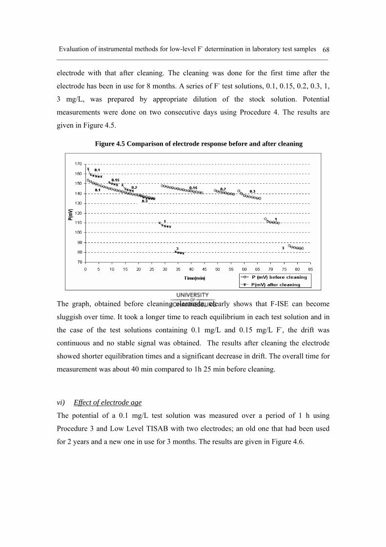
Evaluation of instrumental methods for low-level F- determination in laboratory test samples ______________________________________________________________________________________
68
electrode with that after cleaning. The cleaning was done for the first time after the
electrode has been in use for 8 months. A series of F- test solutions, 0.1, 0.15, 0.2, 0.3, 1,
3 mg/L, was prepared by appropriate dilution of the stock solution. Potential
measurements were done on two consecutive days using Procedure 4. The results are
given in Figure 4.5.
Figure 4.5 Comparison of electrode response before and after cleaning
The graph, obtained before cleaning electrode, clearly shows that F-ISE can become
sluggish over time. It took a longer time to reach equilibrium in each test solution and in
the case of the test solutions containing 0.1 mg/L and 0.15 mg/L F-, the drift was
continuous and no stable signal was obtained. The results after cleaning the electrode
showed shorter equilibration times and a significant decrease in drift. The overall time for
measurement was about 40 min compared to 1h 25 min before cleaning.
vi) Effect of electrode age
The potential of a 0.1 mg/L test solution was measured over a period of 1 h using
Procedure 3 and Low Level TISAB with two electrodes; an old one that had been used
for 2 years and a new one in use for 3 months. The results are given in Figure 4.6.

Evaluation of instrumental methods for low-level F- determination in laboratory test samples ______________________________________________________________________________________
69
Figure 4.6 Comparison electrode responses with respect to electrode age
80
90
100
110
120
130
140
150
0 10 20 30 40 50 60 70Time (min)
Pote
ntia
l (m
V)
P 1 (old) P 2 (old) P 3 (old)P 1 (new) P 2 (new) P 3 (new)
The readings obtained with the old electrode were inconsistent and the drift in the 1st and
3rd run was so severe that no stability was reached. The results obtained with new
electrode, however, showed stable readings, after 18 min for first run, 5 min for second
and 10 min. This result emphasizes the importance of electrode condition on low-level F-
determination.
c. TISAB and calibration study
Accurate calibration is an important factor in the determination of analyte concentration
in any analytical technique. In the case of ISE methods calibration is carried out by
immersing the electrodes in a series of solutions of known concentration and by plotting a
graph of the mV reading versus the log of the activity. According to the Nernst equation,
described in Section 3.1.2.b, this should give a straight line over the whole linear
concentration range. The objectives of the investigation in this section were:
• To study calibration techniques and the effect of different TISAB solutions on the
accuracy of F- determinations
• To investigate multi-standard calibration for low-level F- determinations by
comparing the efficiency of the two TISAB solutions, TISAB III and Low Level
TISAB
• To apply the optimized method to the analysis of low-level F- sample analysis
using deionised water and tap water

Evaluation of instrumental methods for low-level F- determination in laboratory test samples ______________________________________________________________________________________
70
• To investigate the effect of regular electrode cleaning on low-level F-
determination.
i) High-level F- calibration with different TISAB solutions
The calibration graphs, given in Figure 4.7 for the F- concentration range 0.02 mg/L to
1000 mg/L, were obtained using three different TISAB solutions, Low Level TISAB,
TISAB III and TISAB IV. The concentrations in the standard series were: 0.02, 0.05, 0.1,
1, 10, 50, 100 and 1000 mg/L. 20 mL of standard solution without TISAB, 20 mL of
standards and 2 mL of TISAB III, 10mL of standard and 10 mL of TISAB IV and Low
Level TISAB were prepared in 50 mL plastic beakers The potential of standards was
measured from low to high concentration and the meter reading was taken after a
constant value has been attained (drift < 0.1 mV/min). The results obtained from this
experiment are presented in Table 4.3.
Table 4.3 Potential with different TISAB
TISAB type No TISAB TISAB III Low Level TISAB TISAB IV [F] (mg/L) P (mV) P (mV) P (mV) P1 (mV) P2 (mV)
0.02 - 141.3 170.0 60.3 66.0 0.05 - 141.5 168.0 64.3 70.0 0.1 136 135.5 159.2 68.1 71.2 1 81.3 94.0 109.8 64.3 60.3 10 24.3 34.3 50.6 40.0 37.5 50 -16.2 -6.4 9.8 6.3 5.8
100 -33.4 -24.3 -7.5 -11.1 -10.3 1000 -89.5 -82.4 -65.6 -68.6 -67.5
The potential of the 0.02 and 0.05 mg/L F- standard solution, without TISAB, could not
be determined because the potential of these two solutions were consistently decreasing
over a period of an hour. This drift was probably caused by the low ionic strength of 0.02
and 0.05 mg/L F- standards. A stable reading at these levels of F- was obtained after
adding TISAB that increased the ionic strength.
The results are summarized in Table 4.3 and shown in Figure 4.7.

Evaluation of instrumental methods for low-level F- determination in laboratory test samples ______________________________________________________________________________________
71
Figure 4.7 Potential with different types of TISAB
-100
-60
-20
20
60
100
140
1800.01 0.1 1 10 100 1000
[F] logarism scale (mg/l)
P (m
V)
P (mV): No TISABP (mV): T IIIP (mV): LLTP (mV): T IV(1)P (mV): T IV(2)
TIII: TISAB III, LLT: Low Level TISAB, T IV: TISAB IV
As mentioned in Section 3.1.2.b, an electrode is said to have a Nernstian response, when
the potential difference versus the logarithm of the ionic activity of a given species shows
linear relationship. All graphs, except the graphs obtained using TISAB IV, showed the
linear relationship above 0.1 mg/L F- concentration. The graph obtained without TISAB
showed a straight line above 0.1mg/L F-. Although the electrode response showed the
linear relationship, the ISE measurement without TISAB was not practical since it could
not yield stable potentials at lower than 0.1 mg/L F-.
The standard series with TISAB IV was measured twice because the graph showed
excessive curvature at concentrations below 10 mg/L. The duplicate measurement
produced the same result. This meant that TISAB IV could not be used for low-level F-
determination. Orion recommends the use of TISAB IV for the purpose of de-
complexation of Al, but it has been considered unsuitable for the accurate measurement
Evaluation of instrumental methods for low-level F- determination in laboratory test samples ______________________________________________________________________________________
72
of low-level F- concentration (Orion, 1982). This experimental result can be proof of this
statement. It is well known that at low F- levels, the ISE response at pH>8 can be in error
because of interference by hydroxide ions (Orion, 1982). The TISAB IV contains TRIS
buffer for high levels of Al interference at pH 8.5 (see Section 4.2.2). Because of this
high pH value of TISAB IV, the erroneous results obtained for the low-level F-
determination.
The graphs for Low Level TISAB and TISAB III showed straight lines above 0.1mg/L F-
concentration. This meant that both Low Level TISAB and TISAB III could be used for
low-level F- determination.
ii) Low-level F- calibration and sample measurement: TISAB III
Since the focus of this work was on low-level F- determination calibration in the
concentration range 0.01 to 3 mg/L was investigated in detail.
• Low-level calibration
A two-point calibration is sufficient when the measurement is done in the linear range of
the calibration curve. Three or more standards are, however, recommended in order to
confirm the linearity and to detect any errors in diluting the standards. If the curve is non-
linear more standards are needed in order to define the curve in the non-linear range. The
slope of the calibration graph is the mV response per decade of concentration change.
This is typically around 54 mV/decade for monovalent ions and 27 for divalent ions and
will have a negative value for negative ions (Nico, 2000). The calibration graph (Figure
4.7) at low-level concentration shows the curved portion where the electrode response
becomes progressively less as the concentration reduces. In this section, multi-point
calibrations were repeated three times using TISAB III. TISAB III, rather than Low
Level TISAB, was chosen initially since TISAB III contains a de-complexation agent and
is more practical in natural samples that might contain interfering elements such as Al
and Fe. Calibration graphs were obtained by measuring the potential of three different
sets of F- standard solutions in order from low to high concentration. The meter reading
was taken after a constant value has been attained (Drift < 0.1 mV/min).
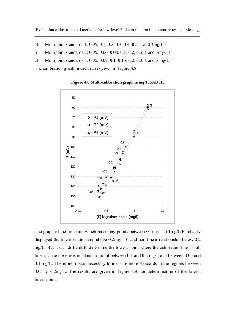
Evaluation of instrumental methods for low-level F- determination in laboratory test samples ______________________________________________________________________________________
73
a) Multipoint standards 1: 0.05, 0.1, 0.2, 0.3, 0.4, 0.5, 1 and 3mg/L F-
b) Multipoint standards 2: 0.05, 0.06, 0.08, 0.1, 0.2, 0.3, 1 and 3mg/L F-
c) Multipoint standards 3: 0.05, 0.07, 0.1, 0.15, 0.2, 0.3, 1 and 3 mg/L F-
The calibration graph in each run is given in Figure 4.8.
Figure 4.8 Multi-calibration graph using TISAB III
3
1
0.5
0.40.3
0.2
0.1
0.05
0.06
0.080.15
0.07
50
60
70
80
90
100
110
120
130
140
150
1600.01 0.1 1 10
[F] logarism scale (mg/l)
P (m
V)
P1 (mV)
P2 (mV)
P3 (mV)
The graph of the first run, which has many points between 0.1mg/L to 1mg/L F-, clearly
displayed the linear relationship above 0.2mg/L F- and non-linear relationship below 0.2
mg/L. But it was difficult to determine the lowest point where the calibration line is still
linear, since there was no standard point between 0.1 and 0.2 mg/L and between 0.05 and
0.1 mg/L. Therefore, it was necessary to measure more standards in the regions between
0.05 to 0.2mg/L. The results are given in Figure 4.8, for determination of the lowest
linear point.
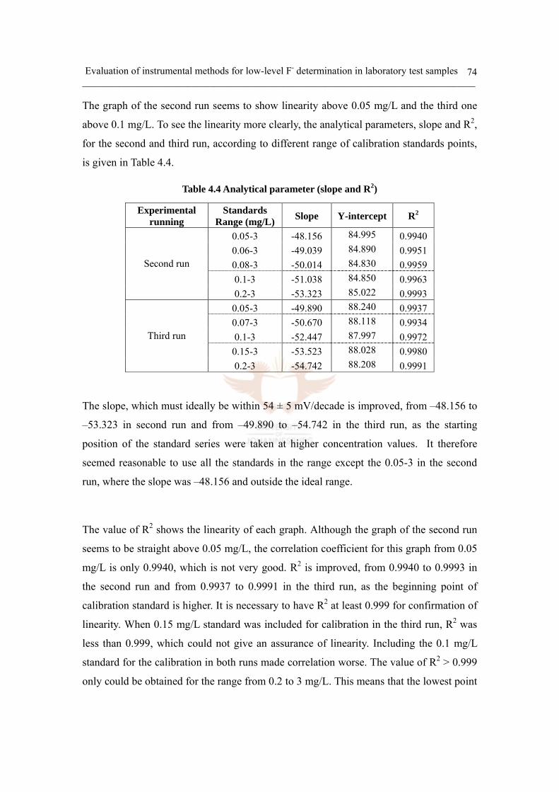
Evaluation of instrumental methods for low-level F- determination in laboratory test samples ______________________________________________________________________________________
74
The graph of the second run seems to show linearity above 0.05 mg/L and the third one
above 0.1 mg/L. To see the linearity more clearly, the analytical parameters, slope and R2,
for the second and third run, according to different range of calibration standards points,
is given in Table 4.4.
Table 4.4 Analytical parameter (slope and R2)
Experimental running
Standards Range (mg/L) Slope Y-intercept R2
0.05-3 -48.156 84.995 0.9940 0.06-3 -49.039 84.890 0.9951 0.08-3 -50.014 84.830 0.9959 0.1-3 -51.038 84.850 0.9963
Second run
0.2-3 -53.323 85.022 0.9993 0.05-3 -49.890 88.240 0.9937 0.07-3 -50.670 88.118 0.9934 0.1-3 -52.447 87.997 0.9972 0.15-3 -53.523 88.028 0.9980
Third run
0.2-3 -54.742 88.208 0.9991
The slope, which must ideally be within 54 ± 5 mV/decade is improved, from –48.156 to
–53.323 in second run and from –49.890 to –54.742 in the third run, as the starting
position of the standard series were taken at higher concentration values. It therefore
seemed reasonable to use all the standards in the range except the 0.05-3 in the second
run, where the slope was –48.156 and outside the ideal range.
The value of R2 shows the linearity of each graph. Although the graph of the second run
seems to be straight above 0.05 mg/L, the correlation coefficient for this graph from 0.05
mg/L is only 0.9940, which is not very good. R2 is improved, from 0.9940 to 0.9993 in
the second run and from 0.9937 to 0.9991 in the third run, as the beginning point of
calibration standard is higher. It is necessary to have R2 at least 0.999 for confirmation of
linearity. When 0.15 mg/L standard was included for calibration in the third run, R2 was
less than 0.999, which could not give an assurance of linearity. Including the 0.1 mg/L
standard for the calibration in both runs made correlation worse. The value of R2 > 0.999
only could be obtained for the range from 0.2 to 3 mg/L. This means that the lowest point
Evaluation of instrumental methods for low-level F- determination in laboratory test samples ______________________________________________________________________________________
75
that can show good linearity is 0.2 mg/L. This fact now presents a problem for
determination of low-level F- samples in the concentration range below 0.2 mg/L. The
influence of the calibration factors, such as slope and R2, were investigated by duplicate
measurement of samples with known concentration.
• Measurement of samples with known concentration in deionised water matrix
Table 4.5 Influence of calibration parameters: linear regression (second run)
Calibration range 0.05-3 mg/L 0.1-3 mg/L 0.2-3 mg/L
Function Y=-48.156x+84.995 Y=-51.038x+84.85 Y=-53.323x+85.022 R2 0.9940 0.9963 0.9993
Known [F] (mg/L)
Calculated[F] (mg/L)
SD (N=2)
% Error
Calculated[F] (mg/L)
SD (N=2)
% Error
Calculated [F] (mg/L)
SD (N=2)
% Error
0.07 0.062 0.005 -10.9 0.072 0.005 3.6 0.082 0.006 16.70.09 0.076 0.006 -15.2 0.088 0.007 -2.6 0.098 0.007 8.9 0.12 0.093 0.001 -22.2 0.106 0.001 -11.7 0.118 0.001 -2.0 0.15 0.114 0.001 -23.8 0.128 0.001 -14.4 0.141 0.001 -5.8 0.18 0.137 0.000 -23.8 0.152 0.000 -15.3 0.166 0.001 -7.5 0.4 0.343 0.005 -14.4 0.362 0.005 -9.6 0.380 0.005 -4.9 0.5 0.442 0.010 -11.5 0.460 0.010 -7.9 0.479 0.010 -4.1 0.8 0.761 0.010 -4.8 0.768 0.010 -4.0 0.783 0.010 -2.2 1.5 1.567 0.000 4.5 1.518 0.000 1.2 1.502 0.000 0.1 2.0 2.123 0.007 6.2 2.021 0.006 1.1 1.976 0.006 -1.2 2.5 2.775 0.009 11.0 2.602 0.008 4.1 2.517 0.008 0.7
Table 4.5 shows the importance of using the proper calibration function for accurate
determination of sample concentration. The results, obtained by using the function for the
range 0.05-3 where the slope was outside the ideal range and the linearity < 0.999, show
large errors. The results for the calibration line based on the range 0.1-3 mg/L and 0.2-3
mg/L are reasonable, but not very good. An additional problem was that sample
concentrations, less than 0.1 mg/L for the calibration range 0.1-3 mg/L and less than 0.2
mg/L for calibration range from 0.2-3 mg/L, could not be determined accurately since
these were out of calibration range. The results in Table 4.6, obtained from the third run,
shows as similar trend as second run.
Evaluation of instrumental methods for low-level F- determination in laboratory test samples ______________________________________________________________________________________
76
Table 4.6 Influence of calibration parameters: linear regression (third run)
Calibration range 0.05-3 mg/L 0.1-3 mg/L 0.2-3 mg/L
Function Y=-48.22x+88.502 Y=-52.447x+87.997 Y=-54.742x+88.208 R2 0.9844 0.9972 0.9991
Known [F] (mg/L)
Calculated[F] (mg/L)
SD (N=2)
% Error
Calculated[F] (mg/L)
SD (N=2)
% Error
Calculated [F] (mg/L)
SD (N=2) % Error
0.06 0.052 0.003 -13.0 0.065 0.003 7.9 0.073 0.003 22.1 0.09 0.073 0.000 -19.4 0.088 0.000 -2.6 0.098 0.000 8.8 0.12 0.095 0.003 -21.2 0.112 0.003 -6.8 0.124 0.004 3.1 0.18 0.148 0.003 -17.9 0.169 0.004 -6.3 0.183 0.004 1.8 0.25 0.211 0.002 -15.5 0.234 0.002 -6.3 0.251 0.002 0.5 0.4 0.349 0.001 -12.8 0.372 0.001 -7.1 0.391 0.001 -2.3 0.5 0.452 0.006 -9.7 0.471 0.004 -5.8 0.490 0.004 -1.9 0.8 0.788 0.016 -1.5 0.785 0.015 -1.8 0.801 0.014 0.1 1.5 1.612 0.000 7.5 1.517 0.000 1.2 1.504 0.000 0.3 2 2.312 0.008 15.6 2.114 0.007 5.7 2.067 0.006 3.3
Therefore a way for the calculation of the sample concentrations below 0.2 mg/L was
investigated, using non-linear regression functions. A summary of the results is given in
Table 4.7 and 4.8.
Table 4.7 F- determination in curvature region (< 0.2 mg/L, second run)
Calibration range Low level between 0.05-0.2 mg/L for measuring < 0.2mg/L sample
Exponential function Polynomial function Linear regression Function
Y=99.279 e-0.2942x Y=704.1x2-331.26x+159.68 Y=-39.047x+94.484 R2 0.9964 0.9999 0.9984
Known [F] (mg/L)
Calculated [F] (mg/L)
SD (N=2)
% Error
Calculated[F] (mg/L)
SD (N=2)
% Error
Calculated [F] (mg/L)
SD (N=2)
% Error
0.07 0.057 0.005 -18.6 0.057 0.006 -18.6 0.057 0.005 -18.30.09 0.073 0.007 -18.9 0.075 0.008 -16.7 0.073 0.008 -18.60.12 0.092 0.001 -23.3 0.095 0.001 -20.8 0.094 0.001 -21.60.15 0.119 0.002 -20.7 0.118 0.001 -21.3 0.121 0.002 -19.60.18 0.150 0.001 -16.7 0.144 0.001 -20.0 0.151 0.001 -16.1
Evaluation of instrumental methods for low-level F- determination in laboratory test samples ______________________________________________________________________________________
77
Table 4.8 F- determination in curvature region (< 0.2 mg/L, third run)
Calibration range Low level between 0.05-0.2 mg/L for measuring < 0.2mg/L sample
Exponential function Polynomial function Linear regression Function
Y=107.09 e-0.2423x Y=148.05x2-169.36x+153.44 Y=-31.118x+104.41
R2 0.9609 0.9933 0.9982 Known
[F] (mg/L) Calculated [F] (mg/L)
SD (N=2)
% Error
Calculated [F] (mg/L)
SD(N=2)
%Error
Calculated [F] (mg/L)
SD (N=2)
% Error
0.06 0.040 0.003 -33.6 0.019 0.006 -69.1 0.033 0.003 -44.30.09 0.062 0.000 -30.9 0.062 0.000 -30.7 0.056 0.000 -38.20.12 0.091 0.004 -24.6 0.101 0.005 -16.2 0.084 0.004 -30.00.18 0.176 0.006 -2.0 0.173 0.004 -3.8 0.168 0.006 -6.9
All the results in both tables are very inaccurate. It meant that other functions, such as
exponential and polynomial, should not be used for determination of F- below 0.2 mg/L
concentration. Since the other functions could not be the solution for the determination of
the F- below 0.2 mg/L, another way, cleaning the electrode, was tried to solve this matter.
• Comparison with regard to electrode cleaning
In this section the effect of the electrode cleaning, referred in Section 4.2.3.b, on
calibration line is discussed. The potential of each standard was measured after cleaning
the electrode and the results together with comparative results before cleaning are shown
in Table 4.9. The calibration standards were chosen as the second run, excluding 0.3
mg/L point.
Table 4.9 Electrode slope with regard to electrode cleaning
Status Before cleaning (second run) After cleaning [F] (mg/L) Log F P (mV) Slope P (mV) Slope
0.05 -1.301 144.8 - 154.0 - 0.06 -1.222 142.4 -30.3 150.5 -44.2 0.08 -1.097 137.8 -36.8 145.0 -44.0 0.1 -1.000 133.5 -44.4 140.3 -48.5 0.2 -0.699 121.6 -39.5 124.7 -51.8 1 0.000 85.9 -51.1 85.9 -55.5 3 0.477 59.0 -56.4 58.6 -57.2
The slope calculation was done by this equation: Slope = ][FLog
Potential∆∆
This table clearly shows that the slope was very much improved after cleaning the
electrode. This proves that electrode cleaning can restore the efficiency of electrode. The
Evaluation of instrumental methods for low-level F- determination in laboratory test samples ______________________________________________________________________________________
78
calibration graph, before cleaning and after cleaning the electrode, is shown in Figure 4.9.
Figure 4.9 Comparison of calibration line in related to electrode cleaning
50
60
70
80
90
100
110
120
130
140
150
1600.01 0.1 1 10
[F] logarism scale (mg/l)
P (m
V)
Before cleaningAfter cleaning
The graph after electrode cleaning clearly shows a better linearity than that obtained
before cleaning. The calibration function and the calculated F- values are given in Table
4.10.
Table 4.10 Sample measurement after cleaning the electrode
Calibration range 0.05-3 ppm 0.08-3 ppm 0.1-3 ppm
Function Y=-53.937x+85.408 Y=-54.989x+85.399 Y=-55.411x+85.449 R2 0.9990 0.9997 0.9998
Known [F] (mg/L)
Calculated [F] (mg/L)
SD (N=2)
% Error
Calculated[F] (mg/L)
SD (N=2)
% Error
Calculated [F] (mg/L)
SD (N=2)
% Error
0.07 0.074 0.003 5.7 0.078 0.003 11.10 0.079 0.003 12.9 0.09 0.090 0.004 0.1 0.094 0.004 4.8 0.096 0.004 6.7
0.15 0.153 0.000 1.7 0.158 0.000 5.4 0.161 0.000 7.3
0.5 0.482 0.017 -3.6 0.489 0.017 -2.2 0.493 0.017 -1.4
0.8 0.788 0.005 -1.5 0.791 0.005 -1.1 0.794 0.005 -0.8
1.5 1.523 0.014 1.6 1.510 0.013 0.7 1.509 0.013 0.6
2 2.089 0.006 4.5 2.059 0.006 3.0 2.052 0.006 2.6

Evaluation of instrumental methods for low-level F- determination in laboratory test samples ______________________________________________________________________________________
79
Seven samples with known F- concentration were measured and their concentrations
calculated based on the different calibration ranges: 0.05-3mg/L, 0.08-3mg/L and 0.1-3
mg/L. Compared to the results in Table 4.6, the linearity was very much improved after
electrode cleaning. The values for R2, were 0.9990, 0.9997 and 0.9998, respectively, in
each calibration range, and were all reasonable good. It means that even the very low
concentration 0.05 mg/L could be included in the calibration function. The slope in each
range, -53.937, -54.989 and –55.411, was and within the ideal range. All calculated F-
values based on these calibration curves were very accurate. These results emphasize the
importance of using a reliable calibration function for the low level F- determination and
the crucial role of electrode conditioning and cleaning in attaining accurate analytical
results.
iii) Low-level F- calibration and sample measurement: Low Level TISAB
• Low-Level calibration
The same calibration experiments were done using Low-Level TISAB instead of TISAB
III and were done after electrode cleaning. The calibration graphs, using TISAB III and
Low Level TISAB, are shown in Figure 4.10 for comparison of TISAB efficiency at low-
level F- concentration.
Figure 4.10 Calibration comparison with TISAB after cleaning
0.2
1
3
0.15
0.070.050.1
3
0.05
0.080.06
0.1
0.2
1
50
60
70
80
90
100
110
120
130
140
150
160
170
1800.01 0.1 1 10
[F] ppm Logarism scale
P(m
V)
Low LevelTISABTISAB III
Evaluation of instrumental methods for low-level F- determination in laboratory test samples ______________________________________________________________________________________
80
The graph for Low Level TISAB displays curvature below 0.1mg/L. Better linearity is
obtained by using TISAB III. TISAB III is therefore the preferred buffer to be used for
low-level F- determination. The results of F- determination in a set of samples with
known concentration using Low Level TISAB are shown in Table 4.11.
• Known sample measurement (Deionised water matrix) Table 4.11 Sample measurement with Low Level TISAB
Calibration range 0.07-3 mg/L 0.1-3 mg/L Function Y=-51.665x+105.57 Y=-53.12x+105.48
R2 0.9962 0.9987 Known
[F] (mg/L) Calculated[F] (mg/L)
SD (N=2)
% Error
Calculated[F] (mg/L)
SD (N=2)
% Error
0.06 0.071 0.000 18.3 0.076 0.000 26.7 0.09 0.094 0.004 4.4 0.100 0.004 11.1 0.12 0.122 0.005 1.7 0.129 0.005 7.5 0.18 0.173 0.009 -3.9 0.181 0.009 0.6 0.25 0.240 0.011 -4.0 0.249 0.011 -0.4 0.4 0.370 0.005 -7.5 0.378 0.005 -5.5 0.5 0.472 0.015 -5.6 0.480 0.015 -4.0 0.8 0.776 0.002 -3.0 0.779 0.002 -2.6 1.5 1.573 0.000 4.9 1.548 0.000 3.2 2 2.169 0.014 8.5 2.115 0.013 5.8
The function for the range 0.07-3mg/L was not suitable for calibration because of their
poor linearity. The calibration lines for the range 0.1-3mg/L were linear and used for
calculation of analyte concentrations. The recoveries, obtained using Low Level TISAB,
were reasonable but not very accurate for the low concentrations.
iv) Low level sample measurement (Tap water matrix)
Up to so far, all the results were obtained in deionised water matrix. However, this matrix
was not relevant to environmental samples. Therefore, further investigations for
environmental samples, using tap water matrix, which was the most accessible, were
done. This section describes the TISAB efficiency, using tap water matrix, in terms of the
Laboratory Fortified Matrix (LFM).
According to the results obtained previously, the lowest concentration positioned on the
linear portion of the calibration graph was 0.05 mg/L for TISAB III and 0.1 mg/L for
Low Level TISAB. The calibration standards, 0.1, 1 and 3mg/L, positioned within the
linear part of the calibration line for both TISAB, were chosen. Raw tap water was taken
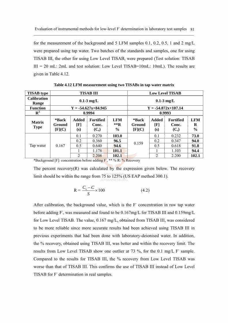
Evaluation of instrumental methods for low-level F- determination in laboratory test samples ______________________________________________________________________________________
81
for the measurement of the background and 5 LFM samples 0.1, 0.2, 0.5, 1 and 2 mg/L
were prepared using tap water. Two batches of the standards and samples, one for using
TISAB III, the other for using Low Level TISAB, were prepared (Test solution: TISAB
III = 20 mL: 2mL and test solution: Low Level TISAB=10mL: 10mL). The results are
given in Table 4.12.
Table 4.12 LFM measurement using two TISABs in tap water matrix
TISAB type TISAB III Low Level TISAB Calibration
Range 0.1-3 mg/L 0.1-3 mg/L
Function Y = -54.627x+84.945 Y = -54.872x+107.14 R2 0.9994 0.9993
Matrix Type
*Back Ground[F](C)
Added [F] (s)
FortifiedConc. (Cs)
LFM **R %
*Back Ground [F](C)
Added [F] (s)
Fortified Conc. (Cs)
LFMR %
0.1 0.270 103.0 0.1 0.232 73.0 0.2 0.360 96.5 0.2 0.347 94.0 0.5 0.640 94.6 0.5 0.618 91.8 1 1.178 101.1 1 1.103 94.4
Tap water
0.167
2 2.208 102.1
0.159
2 2.200 102.1*Background [F]: concentration before adding F-, ** % R: % Recovery
The percent recovery(R) was calculated by the expression given below. The recovery
limit should be within the range from 75 to 125% (US EAP method 300.1).
R = 100×−S
CCs (4.2)
After calibration, the background value, which is the F- concentration in raw tap water
before adding F-, was measured and found to be 0.167mg/L for TISAB III and 0.159mg/L
for Low Level TISAB. The value, 0.167 mg/L, obtained from TISAB III, was considered
to be more reliable since more accurate results had been achieved using TISAB III in
previous experiments that had been done with laboratory-deionised water. In addition,
the % recovery, obtained using TISAB III, was better and within the recovery limit. The
results from Low Level TISAB show one outlier at 73 %, for the 0.1 mg/L F- sample.
Compared to the results for TISAB III, the % recovery from Low Level TISAB was
worse than that of TISAB III. This confirms the use of TISAB III instead of Low Level
TISAB for F- determination in real samples.
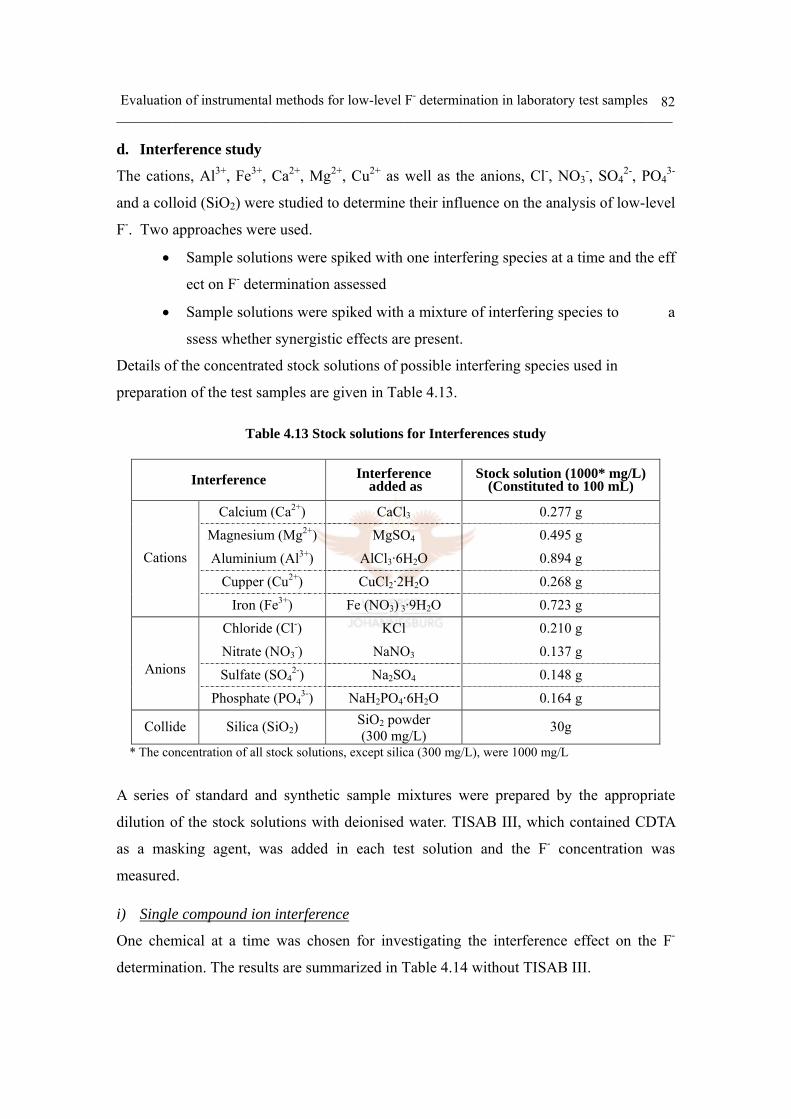
Evaluation of instrumental methods for low-level F- determination in laboratory test samples ______________________________________________________________________________________
82
d. Interference study
The cations, Al3+, Fe3+, Ca2+, Mg2+, Cu2+ as well as the anions, Cl-, NO3-, SO4
2-, PO43-
and a colloid (SiO2) were studied to determine their influence on the analysis of low-level
F-. Two approaches were used.
• Sample solutions were spiked with one interfering species at a time and the eff
ect on F- determination assessed
• Sample solutions were spiked with a mixture of interfering species to a
ssess whether synergistic effects are present.
Details of the concentrated stock solutions of possible interfering species used in
preparation of the test samples are given in Table 4.13.
Table 4.13 Stock solutions for Interferences study
Interference Interference added as
Stock solution (1000* mg/L) (Constituted to 100 mL)
Calcium (Ca2+) CaCl3 0.277 g Magnesium (Mg2+) MgSO4 0.495 g
Aluminium (Al3+) AlCl3·6H2O 0.894 g
Cupper (Cu2+) CuCl2·2H2O 0.268 g
Cations
Iron (Fe3+) Fe (NO3) 3·9H2O 0.723 g Chloride (Cl-) KCl 0.210 g
Nitrate (NO3-) NaNO3 0.137 g
Sulfate (SO42-) Na2SO4 0.148 g
Anions
Phosphate (PO43-) NaH2PO4·6H2O 0.164 g
Collide Silica (SiO2) SiO2 powder (300 mg/L) 30g
* The concentration of all stock solutions, except silica (300 mg/L), were 1000 mg/L
A series of standard and synthetic sample mixtures were prepared by the appropriate
dilution of the stock solutions with deionised water. TISAB III, which contained CDTA
as a masking agent, was added in each test solution and the F- concentration was
measured.
i) Single compound ion interference
One chemical at a time was chosen for investigating the interference effect on the F-
determination. The results are summarized in Table 4.14 without TISAB III.
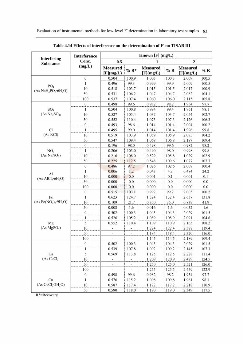
Evaluation of instrumental methods for low-level F- determination in laboratory test samples ______________________________________________________________________________________
83
Table 4.14 Effects of interference on the determination of F- no TISAB III
Known [F] (mg/L) 0.5 1 2
Interfering Substance
Interference Conc. (mg/L)
Measured [F](mg/L) % R* Measured
[F](mg/L) % R Measured [F](mg/L) % R
0 0.504 100.9 1.003 100.3 2.009 100.51 0.496 99.3 0.999 99.9 2.009 100.5
10 0.518 103.7 1.015 101.5 2.017 100.950 0.531 106.2 1.047 104.7 2.082 104.1
PO4 (As NaH2PO4·6H2O)
100 0.537 107.4 1.060 106.0 2.115 105.80 0.498 99.6 0.982 98.2 1.954 97.71 0.504 100.8 0.994 99.4 1.961 98.1
10 0.527 105.4 1.037 103.7 2.054 102.7SO4
(As Na2SO4) 50 0.552 110.4 1.073 107.3 2.126 106.30 0.493 98.6 1.014 101.4 2.004 100.21 0.495 99.0 1.014 101.4 1.996 99.8
10 0.519 103.9 1.059 105.9 2.085 104.2Cl
(As KCl) 50 0.547 109.4 1.068 106.8 2.187 109.40 0.196 98.0 0.498 99.6 0.982 98.21 0.206 103.0 0.490 98.0 0.998 99.8
10 0.216 108.0 0.529 105.8 1.029 102.9NO3
(As NaNO3) 50 0.225 112.5 0.548 109.6 1.077 107.70 0.486 97.2 1.026 102.6 2.008 100.41 0.006 1.2 0.043 4.3 0.484 24.2
10 0.000 0.0 0.001 0.1 0.001 0.150 0.000 0.0 0.000 0.0 0.000 0.0
Al (As AlCl3·6H2O)
100 0.000 0.0 0.000 0.0 0.000 0.00 0.515 103.1 0.992 99.2 2.005 100.21 0.623 124.7 1.324 132.4 2.637 131.8
10 0.109 21.7 0.350 35.0 0.839 41.9Fe
(As Fe(NO3)3·9H2O) 50 0.008 1.6 0.016 1.6 0.032 1.60 0.502 100.3 1.043 104.3 2.029 101.51 0.526 105.2 1.089 108.9 2.091 104.65 0.552 110.4 1.109 110.9 2.163 108.2
10 - - 1.224 122.4 2.388 119.450 - - 1.184 118.4 2.320 116.0
Mg (As MgSO4)
100 - - 1.145 114.5 2.189 109.40 0.502 100.3 1.043 104.3 2.029 101.51 0.539 107.8 1.092 109.2 2.145 107.35 0.569 113.8 1.125 112.5 2.228 111.4
10 - - 1.209 120.9 2.489 124.550 - - 1.250 125.0 2.521 126.0
Ca (As CaCl3)
100 - - 1.255 125.5 2.459 122.90 0.498 99.6 0.982 98.2 1.954 97.71 0.576 115.2 1.098 109.8 1.961 98.1
10 0.587 117.4 1.172 117.2 2.218 110.9Cu
(As CuCl2·2H2O) 50 0.590 118.0 1.190 119.0 2.349 117.5
R*=Recovery

Evaluation of instrumental methods for low-level F- determination in laboratory test samples ______________________________________________________________________________________
84
Table 4.14 shows the effect of a single compound interference on the determination of F-
without TISAB III. All the anion interferences show positive errors and the recoveries are
over 100 %. Considering the effect of ionic strength and activity, the % recoveries should
have been less than 100% (see Section 3.1.2.a). When the ionic strength increases an ion
loses some of its effectiveness, and its activity coefficient decreases. This indicates that
there must be another reason for the over-estimation of F- in the presence of anions tested.
The possible reason could be the F- electrode response to other anions when the
concentration of anion interference is high enough.
Among all the cation interferences, Al showed the most serious influence on
determination of F-. The % recoveries of 0.5 mg/L F- in presence of Al interference were
1.2 % for 1 mg/L Al, 0 % for 10, 50 and 100mg/L Al. Table 4.15 shows that ionic
strength effects can only account for a very small part of the observed interference.
Table 4.15 Ionic strength and activity coefficient for Al interference
[F] (mg/L) Added [Al] (mg/L) *Ionic strengthµ
**Activity coefficient γ
Error (-) in Concentration
1 0.00023 0.983 1.74 % 10 0.00211 0.950 4.99 % 50 0.01047 0.898 10.19 % 0.5
100 0.02092 0.865 13.54 % *Ionic strength was calculated by the equation 3.2 in Section 3.1.2.a.i
**Activity coefficient was calculated by the Debye-Hückel equation (see Section 3.1.2.a.ii)
It is well known that Al ions readily form stable complexes with F- ions (Vanlengenhaghe,
1966; Durrant and Durrant, 1970; Srinivasan and Rechnitz, 1988). Several different
forms of Al-F can be found with various F/Al ratios (Wells, 1975). Durrant (1970)
reported that one Al ion in the complex structure is surrounded by a maximum of 6
octahedrally arranged F- ions. Therefore, the significant interference by Al ions is caused
by the strong affinity of F- ions for Al ions and the formation of an octahedral structure of
Al-F with which one Al ion can combine up to a maximum of six F- ions, unless
decomplexing agents such as CDTA, the citrate-nitrate medium, are used (Nakajima,
1997). Fe also seemed to cause a negative error, except at 1 mg/L Fe, which shows a
positive error. This positive error was caused by the NO3- interference, which came from
the chemical (Fe (NO3)3·9H2O) used to prepare the Fe interference stock solution. The

Evaluation of instrumental methods for low-level F- determination in laboratory test samples ______________________________________________________________________________________
85
extent of the Fe interference is much less than that of Al. The reason is the much smaller
stability constants for the Fe complexes with F- (see Table 4.16).
Table 4.16 The log of stability constant* for F- ligand
Metal Stability constant* Al3+ Fe3+ Fe2+ Mg2+ Ca2+ Cu2+
Log K1 6.10 5.16 0.83 1.32 0.70 0.84
Log K2 4.93 3.91 - - - -
Log K3 6.69 2.93 - - - -
Log K4 2.50 - - - - -
* From Stability Constants of Metal-Ion Complexes Part A INORGANIC LIGANDS (Erik H., 1982)
The stability constants for both Fe2+ and Fe3+ complexes with F- are less than that of Al.
At the1mg/L Fe level, the % recoveries were 124.7%, 132.4% and 131.8 % respectively.
This overestimation shows that the effect of the Fe-F complex, at 1mg/L Fe, was less
than that of anion (NO3-) effect that caused the overestimation. As the Fe concentration
increased, the % recoveries were decreased.
Ca2+, Mg2+ and Cu2+, in Table 4.14, show a positive error. This positive error could not
be interpreted in terms of ionic strength and activity, because the increase of the ionic
strength causes a decrease in the activity, which should lead to a negative error. All the
positive errors for these cation interferences seem to be caused by anion interference
from the counter ion. The logs of stability constants of these cations (see Table 4.16)
were 1.32, 0.70 and 0.84. This meant that Ca2+, Mg2+ and Cu2+ did not form strong
fluoro-complexes like Al3+ or Fe3+. These cations, Ca2+, Mg2+ and Cu2+, therefore did not
present major problems on the F- determination. The results, obtained by using TISAB III,
are summarized in Table 4.17.
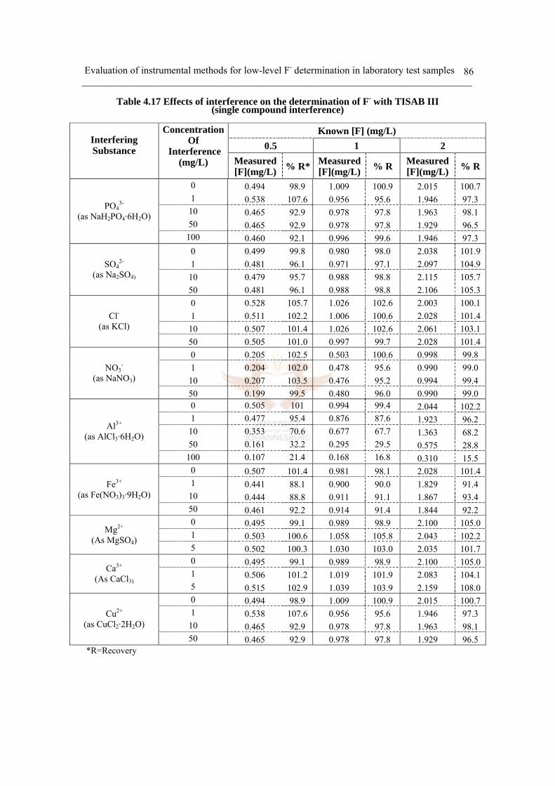
Evaluation of instrumental methods for low-level F- determination in laboratory test samples ______________________________________________________________________________________
86
Table 4.17 Effects of interference on the determination of F- with TISAB III (single compound interference)
Known [F] (mg/L) 0.5 1 2 Interfering
Substance
Concentration Of
Interference (mg/L)
Measured [F](mg/L) % R* Measured
[F](mg/L) % R Measured [F](mg/L) % R
0 0.494 98.9 1.009 100.9 2.015 100.71 0.538 107.6 0.956 95.6 1.946 97.310 0.465 92.9 0.978 97.8 1.963 98.150 0.465 92.9 0.978 97.8 1.929 96.5
PO43-
(as NaH2PO4·6H2O)
100 0.460 92.1 0.996 99.6 1.946 97.30 0.499 99.8 0.980 98.0 2.038 101.91 0.481 96.1 0.971 97.1 2.097 104.910 0.479 95.7 0.988 98.8 2.115 105.7
SO42-
(as Na2SO4)
50 0.481 96.1 0.988 98.8 2.106 105.30 0.528 105.7 1.026 102.6 2.003 100.11 0.511 102.2 1.006 100.6 2.028 101.410 0.507 101.4 1.026 102.6 2.061 103.1
Cl-
(as KCl)
50 0.505 101.0 0.997 99.7 2.028 101.40 0.205 102.5 0.503 100.6 0.998 99.81 0.204 102.0 0.478 95.6 0.990 99.010 0.207 103.5 0.476 95.2 0.994 99.4
NO3-
(as NaNO3)
50 0.199 99.5 0.480 96.0 0.990 99.00 0.505 101 0.994 99.4 2.044 102.21 0.477 95.4 0.876 87.6 1.923 96.210 0.353 70.6 0.677 67.7 1.363 68.250 0.161 32.2 0.295 29.5 0.575 28.8
Al3+
(as AlCl3·6H2O)
100 0.107 21.4 0.168 16.8 0.310 15.50 0.507 101.4 0.981 98.1 2.028 101.41 0.441 88.1 0.900 90.0 1.829 91.410 0.444 88.8 0.911 91.1 1.867 93.4
Fe3+
(as Fe(NO3)3·9H2O) 50 0.461 92.2 0.914 91.4 1.844 92.20 0.495 99.1 0.989 98.9 2.100 105.01 0.503 100.6 1.058 105.8 2.043 102.2
Mg2+
(As MgSO4) 5 0.502 100.3 1.030 103.0 2.035 101.70 0.495 99.1 0.989 98.9 2.100 105.01 0.506 101.2 1.019 101.9 2.083 104.1
Ca3+
(As CaCl3) 5 0.515 102.9 1.039 103.9 2.159 108.00 0.494 98.9 1.009 100.9 2.015 100.71 0.538 107.6 0.956 95.6 1.946 97.310 0.465 92.9 0.978 97.8 1.963 98.1
Cu2+
(as CuCl2·2H2O) 50 0.465 92.9 0.978 97.8 1.929 96.5
*R=Recovery

Evaluation of instrumental methods for low-level F- determination in laboratory test samples ______________________________________________________________________________________
87
Compared to the previous results in Table 4.14 (without TISAB III), all the results in this
table display better recoveries because of using TISAB III. Over-estimation from the
anion interferences could be corrected by adding TISAB III.
However, the cation interferences, Al and Fe, were problematic even after adding TISAB
III. The following histograms, obtained from the experimental results, (Figure 4.11 and
4.12) show the efficiency of TISAB III for de-complexation of Al and Fe at the level of 1
mg/L Al and 10mg/L Fe.
Figure 4.11 TISAB efficiency for F- determination in presence of Al*
0
20
40
60
80
100
0.5 1 2
[F] (mg/l)
Fluo
ride
Rec
over
y(%
)
NoTISAB With TIII
*Al concentration = 1 mg/L
Figure 4.12 TISAB efficiency for F- determination in presence of Fe*
0
20
40
60
80
100
0.5 1 2
[F] (mg/l)
Fluo
ride
Rec
over
y(%
)
NoTISAB With TIII
* Fe concentration = 10 mg/L
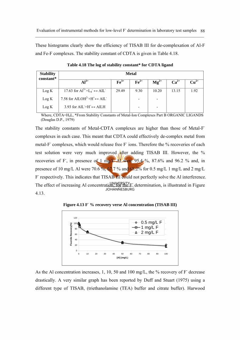
Evaluation of instrumental methods for low-level F- determination in laboratory test samples ______________________________________________________________________________________
88
These histograms clearly show the efficiency of TISAB III for de-complexation of Al-F
and Fe-F complexes. The stability constant of CDTA is given in Table 4.18.
Table 4.18 The log of stability constant* for CDTA ligand
Metal Stability constant*
Al3+ Fe3+ Fe2+ Mg2+ Ca2+ Cu2+
Log K 17.63 for Al3++L4- ↔ AlL- 29.49 9.30 10.20 13.15 1.92
Log K 7.58 for AlLOH2-+H+↔ AlL- - -
Log K 3.93 for AlL-+H+↔ AlLH - -
Where, CDTA=H4L, *From Stability Constants of Metal-Ion Complexes Part B ORGANIC LIGANDS (Douglas D.P., 1979)
The stability constants of Metal-CDTA complexes are higher than those of Metal-F-
complexes in each case. This meant that CDTA could effectively de-complex metal from
metal-F- complexes, which would release free F- ions. Therefore the % recoveries of each
test solution were very much improved after adding TISAB III. However, the %
recoveries of F-, in presence of 1 mg/L Al were 95.4 %, 87.6% and 96.2 % and, in
presence of 10 mg/L Al were 70.6 %, 67.7 % and 68.2% for 0.5 mg/L 1 mg/L and 2 mg/L
F- respectively. This indicates that TISAB III could not perfectly solve the Al interference.
The effect of increasing Al concentration, for the F- determination, is illustrated in Figure
4.13.
Figure 4.13 F- % recovery verse Al concentration (TISAB III)
0
20
40
60
80
100
120
0 10 20 30 40 50 60 70 80 90 100
[Al] (mg/L)
Fluo
ride
Rec
over
y(%
) 0.5 mg/L F1 mg/L F2 mg/L F
As the Al concentration increases, 1, 10, 50 and 100 mg/L, the % recovery of F- decrease
drastically. A very similar graph has been reported by Duff and Stuart (1975) using a
different type of TISAB, (triethanolamine (TEA) buffer and citrate buffer). Harwood
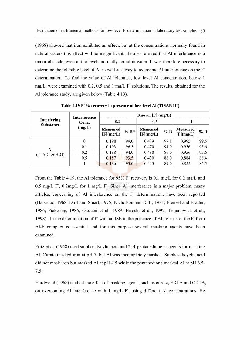
Evaluation of instrumental methods for low-level F- determination in laboratory test samples ______________________________________________________________________________________
89
(1968) showed that iron exhibited an effect, but at the concentrations normally found in
natural waters this effect will be insignificant. He also referred that Al interference is a
major obstacle, even at the levels normally found in water. It was therefore necessary to
determine the tolerable level of Al as well as a way to overcome Al interference on the F-
determination. To find the value of Al tolerance, low level Al concentration, below 1
mg/L, were examined with 0.2, 0.5 and 1 mg/L F- solutions. The results, obtained for the
Al tolerance study, are given below (Table 4.19).
Table 4.19 F- % recovery in presence of low-level Al (TISAB III)
Known [F] (mg/L) 0.2 0.5 1 Interfering
Substance
Interference Conc. (mg/L)
Measured [F](mg/L) % R* Measured
[F](mg/L) % R Measured [F](mg/L) % R
0 0.198 99.0 0.489 97.8 0.995 99.50.1 0.193 96.5 0.470 94.0 0.956 95.60.2 0.188 94.0 0.430 86.0 0.956 95.60.5 0.187 93.5 0.430 86.0 0.884 88.4
Al (as AlCl3·6H2O)
1 0.186 93.0 0.445 89.0 0.855 85.5
From the Table 4.19, the Al tolerance for 95% F- recovery is 0.1 mg/L for 0.2 mg/L and
0.5 mg/L F-, 0.2mg/L for 1 mg/L F-. Since Al interference is a major problem, many
articles, concerning of Al interference on the F- determination, have been reported
(Harwood, 1968; Duff and Stuart, 1975; Nicholson and Duff, 1981; Frenzel and Brätter,
1986; Pickering, 1986; Okutani et al., 1989; Hiroshi et al., 1997; Trojanowicz et al.,
1998). In the determination of F- with an ISE in the presence of Al, release of the F- from
Al-F complex is essential and for this purpose several masking agents have been
examined.
Fritz et al. (1958) used sulphosalycylic acid and 2, 4-pentanedione as agents for masking
Al. Citrate masked iron at pH 7, but Al was incompletely masked. Sulphosalicyclic acid
did not mask iron but masked Al at pH 4.5 while the pentanedione masked Al at pH 6.5-
7.5.
Hardwood (1968) studied the effect of masking agents, such as citrate, EDTA and CDTA,
on overcoming Al interference with 1 mg/L F-, using different Al concentrations. He

Evaluation of instrumental methods for low-level F- determination in laboratory test samples ______________________________________________________________________________________
90
found citrate and EDTA were not satisfactory, while CDTA released F- at Al levels up to
3 or 5 mg/L, depending on the accuracy required. The result obtained by Crosby et al.
(1968) agreed with the fact that citrate is not completely reliable for masking Al.
However, the buffer recommended by them, contained EDTA.
Yuchi et al. (1986), on the other hand, reported that citrate is more effective than DCTA
or EDTA for masking Al, because it does not form appreciable amounts of mixed ligand
complexes with Al and F- at pH 6.
Nakajima et al. (1997) suggested that when a solution contains more than 0.5 mg/L F- and
up to 20 mg/L Al, the use of TISAB with sodium citrate-potassium nitrate was
recommended. On the other hand, when a solution contains more than 0.1 mg/L F- and
less than 5 mg/L Al, TISAB contained CDTA could be used.
The different views expressed, arise in part from the fact that the degree of release varies
with buffer pH. At low F- levels, the ISE response at pH>8 can be in error because of
interference by hydroxide ions (Orion, 1982), but use of higher pH reduces Al
interference. At pH ~8, recommended masking agents include 0.25 M sodium citrate
(Vickery and Vickery, 1976), 1M sodium citrate (Oliver and Clayton, 1970) and
tris(hydroxymethyl)aminomethane (Kauranen, 1977). At pH 12, formation of the
tetrahydroxo-aluminate ion tends to eliminate Al interference (Oliver and Clayton, 1970).
Okutani et al. (1989) has been illustrated the effect of pH on masking of Al, using citrate
buffer. The masking ability of citrate is markedly enhanced by increase in pH from 6.0 to
8.5, and even at a concentration of 0.015 M (405 mg/L) Al can be masked at pH 8.5 with
citrate in the determination of 0.2-2.0 µg/mL F-. Based on this fact, they developed a
method, which could mask large amounts of Al and determine low levels of F- in natural
waters after co-precipitation with aluminum phosphate.
Nicholson and Duff (1981) also have compared the effectiveness of various masking
agents, which were Citrate, CDTA, Tiron, Mannitol, Salicylate and Tris(hydroxymethyl)
methylamine. Of all the buffer masking agent combinations examined, tri-Ammonium
citrate (TAC) buffer, employing CDTA and tri-ammonium citrate as complexing agents,
was most efficient in terms of masking ability. At 1 mg/L F-, an Al concentration up to

Evaluation of instrumental methods for low-level F- determination in laboratory test samples ______________________________________________________________________________________
91
100 mg/L was tolerated for 95% recovery. This was greatly superior to TISAB III, which
at the same F- concentration and recovery level tolerated only 2.7 mg/L Al. An important
aspect is the time required for the masking of Al to become complete. In their detailed
study, they noted that 24 hours following buffer addition, would, for each species and
each buffer, at 1 mg/L F- be beneficial in terms of an increased F- recovery. These results
were very remarkable so that the experiments were repeated to confirm. Firstly, TAC
buffer was prepared using TISAB III. The calculated value of TAC was 1M. The results
of F- determination with this buffer as well as the previous work from Table 4.17 are
summarized in Table 4.20.
Table 4.20 The efficiency of TAC buffer on the F- determination
1 mg/L F-
TISAB Type *TISAB III TAC buffer
Interfering Substance
InterferenceConc. (mg/L)
Measured [F](mg/L) % R*
Measured [F](mg/L) % R
0 0.994 99.4 1.024 102.4 1 0.876 87.6 0.962 96.2 5 - - 0.942 94.2
10 0.677 67.7 0.904 90.4 50 0.295 29.5 0.666 66.6
Al (as AlCl3·6H2O)
100 0.168 16.8 0.509 50.9 * TISAB III results was cited from Table 4.17
This result obviously shows that Al concentration up to 5 mg/L was tolerated for 94%
recovery at 1 mg/L F-. Compared to the previous work in Table 4.17, the F- recovery was
very much improved employing TAC buffer. Although this tolerance value was far less
than that of the article, which is 100 mg/L Al, this TISAB can be applied to F-
determinations in the environmental samples that contain Al below 1 mg/L. This
experiment confirmed the fact that TAC buffer is greatly superior to TISAB III in terms
of masking Al interference.
Secondly, the experiment was designed to confirm the effectiveness of time allowance
using TISAB III. A reference solution, 1 mg/L F-(Fr) and a sample solution, mixture of
1mg/L F- and 1 mg/L Al (Fs) were made up. After calibration, using standards 0.1, 0.5
and 3 mg/L F- concentrations of these two solutions were determined at several times
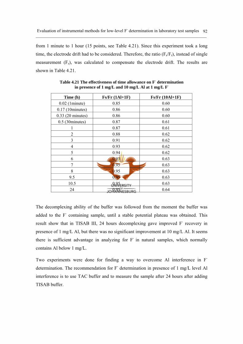
Evaluation of instrumental methods for low-level F- determination in laboratory test samples ______________________________________________________________________________________
92
from 1 minute to 1 hour (15 points, see Table 4.21). Since this experiment took a long
time, the electrode drift had to be considered. Therefore, the ratio (Fs/Fr), instead of single
measurement (Fs), was calculated to compensate the electrode drift. The results are
shown in Table 4.21.
Table 4.21 The effectiveness of time allowance on F- determination in presence of 1 mg/L and 10 mg/L Al at 1 mg/L F-
Time (h) Fs/Fr (1Al+1F) Fs/Fr (10Al+1F) 0.02 (1minute) 0.85 0.60
0.17 (10minutes) 0.86 0.60 0.33 (20 minutes) 0.86 0.60 0.5 (30minutes) 0.87 0.61
1 0.87 0.61 2 0.88 0.62 3 0.91 0.62 4 0.93 0.62 5 0.94 0.62 6 0.93 0.63 7 0.95 0.63 8 0.95 0.63
9.5 0.95 0.63 10.5 0.95 0.63 24 0.95 0.64
The decomplexing ability of the buffer was followed from the moment the buffer was
added to the F- containing sample, until a stable potential plateau was obtained. This
result show that in TISAB III, 24 hours decomplexing gave improved F- recovery in
presence of 1 mg/L Al, but there was no significant improvement at 10 mg/L Al. It seems
there is sufficient advantage in analyzing for F- in natural samples, which normally
contains Al below 1 mg/L.
Two experiments were done for finding a way to overcome Al interference in F-
determination. The recommendation for F- determination in presence of 1 mg/L level Al
interference is to use TAC buffer and to measure the sample after 24 hours after adding
TISAB buffer.

Evaluation of instrumental methods for low-level F- determination in laboratory test samples ______________________________________________________________________________________
93
ii) Single compound colloid interference
Colloid particles usually occur in natural samples. A colloid is a system in which finely
divided particles, which are approximately < 0.1 µm in size, are dispersed within a
continuous medium in a manner that prevents them from being filtered easily or settled
rapidly. 60 mg/L colloidal SiO2 was chosen to check the effect of the colloid interference
(Table 4.22).
Table 4.22 Effects of colloid interference on the determination of F- with TISAB III
Known [F] (mg/L) 0.2 0.5 1 Interfering
Substance
Interference Conc. (mg/L)
Measured [F](mg/L) % R Measured
[F](mg/L) % R Measured [F](mg/L) % R
0 0.196 97.8 0.485 96.9 0.982 98.260 0.201 100.7 0.490 97.9 1.003 100.3SiO2
(As SiO2 powder) 180 0.195 97.5 0.480 96.0 0.973 97.3
This indicates that SiO2 colloidal particle has little effect on the F- result, even at 180
mg/L.
iii) Multi-compound interferences
Up to so far, single compound ion and colloid interference on F- determination was tested.
However, there were numerous elements in the natural sample. So sample solutions were
spiked with more than 2 compounds, with various mixtures of interfering species, to
assess whether synergistic effects are present. The concentrations of interfering
substances were Al3+ 1mg/L, Mg2+ 10mg/L, Ca2+ 10mg/L, Fe2+ 1 mg/L and PO43-
10mg/L at 0.2, 0.5 and 1 mg/L F-.
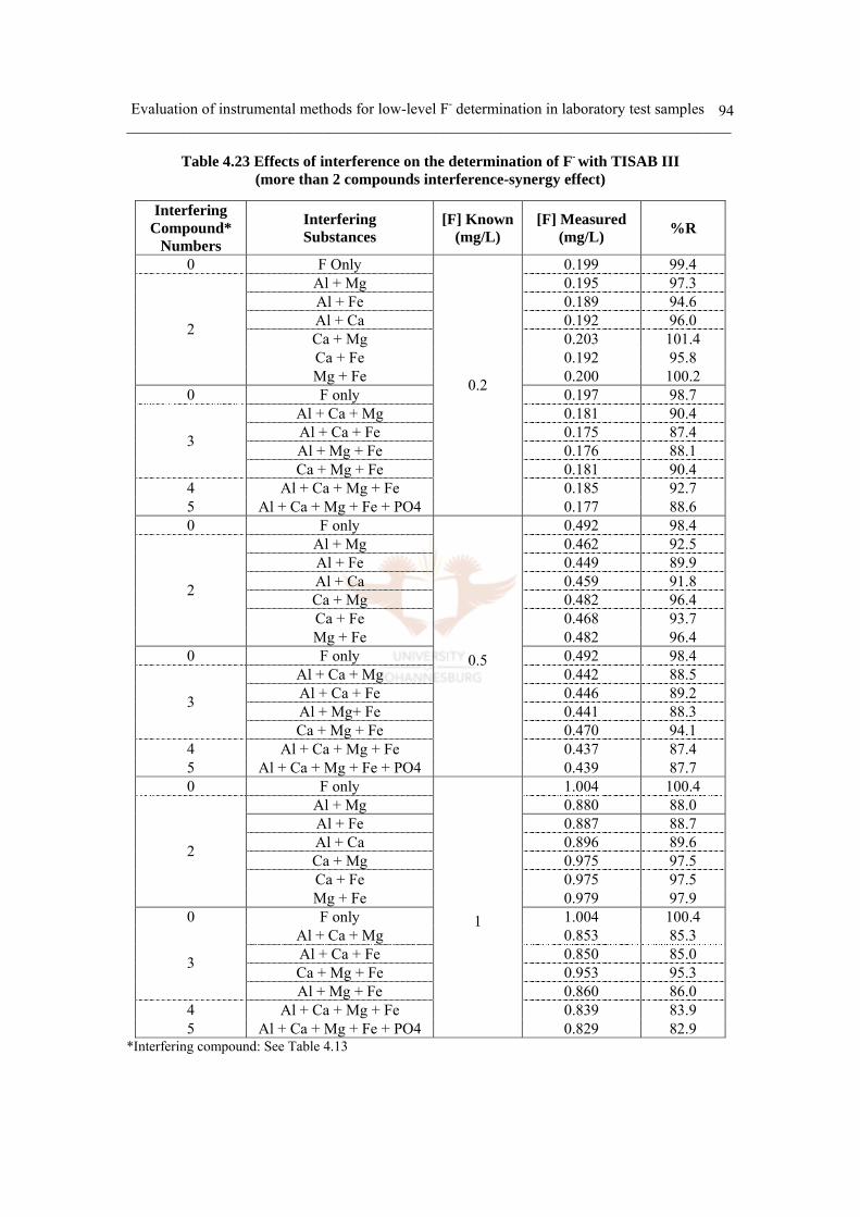
Evaluation of instrumental methods for low-level F- determination in laboratory test samples ______________________________________________________________________________________
94
Table 4.23 Effects of interference on the determination of F- with TISAB III (more than 2 compounds interference-synergy effect)
Interfering Compound*
Numbers
Interfering Substances
[F] Known(mg/L)
[F] Measured (mg/L) %R
0 F Only 0.199 99.4 Al + Mg 0.195 97.3 Al + Fe 0.189 94.6 Al + Ca 0.192 96.0 Ca + Mg 0.203 101.4 Ca + Fe 0.192 95.8
2
Mg + Fe 0.200 100.2 0 F only 0.197 98.7
Al + Ca + Mg 0.181 90.4 Al + Ca + Fe 0.175 87.4 Al + Mg + Fe 0.176 88.1 3
Ca + Mg + Fe 0.181 90.4 4 Al + Ca + Mg + Fe 0.185 92.7 5 Al + Ca + Mg + Fe + PO4
0.2
0.177 88.6 0 F only 0.492 98.4
Al + Mg 0.462 92.5 Al + Fe 0.449 89.9 Al + Ca 0.459 91.8 Ca + Mg 0.482 96.4 Ca + Fe 0.468 93.7
2
Mg + Fe 0.482 96.4 0 F only 0.492 98.4
Al + Ca + Mg 0.442 88.5 Al + Ca + Fe 0.446 89.2 Al + Mg+ Fe 0.441 88.3 3
Ca + Mg + Fe 0.470 94.1 4 Al + Ca + Mg + Fe 0.437 87.4 5 Al + Ca + Mg + Fe + PO4
0.5 0.439 87.7
0 F only 1.004 100.4 Al + Mg 0.880 88.0 Al + Fe 0.887 88.7 Al + Ca 0.896 89.6 Ca + Mg 0.975 97.5 Ca + Fe 0.975 97.5
2
Mg + Fe 0.979 97.9 0 F only 1.004 100.4
Al + Ca + Mg 0.853 85.3 Al + Ca + Fe 0.850 85.0 Ca + Mg + Fe 0.953 95.3 3
Al + Mg + Fe 0.860 86.0 4 Al + Ca + Mg + Fe 0.839 83.9 5 Al + Ca + Mg + Fe + PO4
1
0.829 82.9
*Interfering compound: See Table 4.13
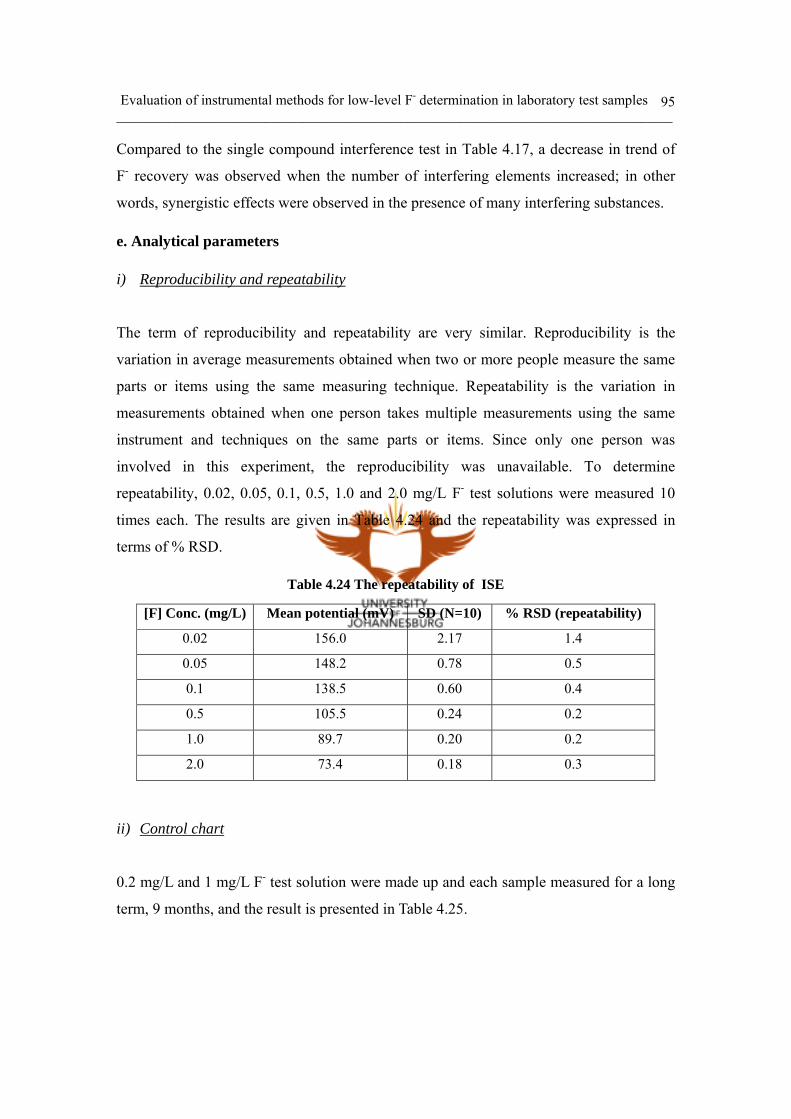
Evaluation of instrumental methods for low-level F- determination in laboratory test samples ______________________________________________________________________________________
95
Compared to the single compound interference test in Table 4.17, a decrease in trend of
F- recovery was observed when the number of interfering elements increased; in other
words, synergistic effects were observed in the presence of many interfering substances.
e. Analytical parameters
i) Reproducibility and repeatability
The term of reproducibility and repeatability are very similar. Reproducibility is the
variation in average measurements obtained when two or more people measure the same
parts or items using the same measuring technique. Repeatability is the variation in
measurements obtained when one person takes multiple measurements using the same
instrument and techniques on the same parts or items. Since only one person was
involved in this experiment, the reproducibility was unavailable. To determine
repeatability, 0.02, 0.05, 0.1, 0.5, 1.0 and 2.0 mg/L F- test solutions were measured 10
times each. The results are given in Table 4.24 and the repeatability was expressed in
terms of % RSD.
Table 4.24 The repeatability of ISE
[F] Conc. (mg/L) Mean potential (mV) SD (N=10) % RSD (repeatability)
0.02 156.0 2.17 1.4
0.05 148.2 0.78 0.5
0.1 138.5 0.60 0.4
0.5 105.5 0.24 0.2
1.0 89.7 0.20 0.2
2.0 73.4 0.18 0.3
ii) Control chart
0.2 mg/L and 1 mg/L F- test solution were made up and each sample measured for a long
term, 9 months, and the result is presented in Table 4.25.
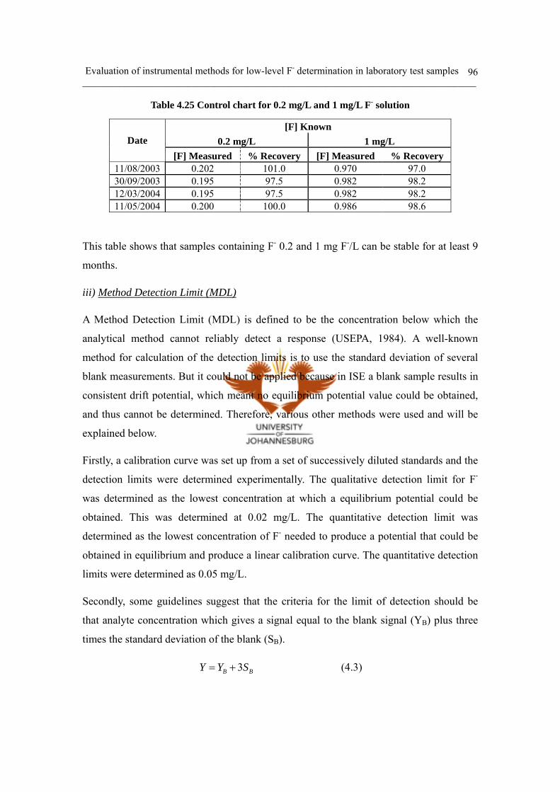
Evaluation of instrumental methods for low-level F- determination in laboratory test samples ______________________________________________________________________________________
96
Table 4.25 Control chart for 0.2 mg/L and 1 mg/L F- solution
[F] Known 0.2 mg/L 1 mg/L Date
[F] Measured % Recovery [F] Measured % Recovery 11/08/2003 0.202 101.0 0.970 97.0 30/09/2003 0.195 97.5 0.982 98.2 12/03/2004 0.195 97.5 0.982 98.2 11/05/2004 0.200 100.0 0.986 98.6
This table shows that samples containing F- 0.2 and 1 mg F-/L can be stable for at least 9
months.
iii) Method Detection Limit (MDL)
A Method Detection Limit (MDL) is defined to be the concentration below which the
analytical method cannot reliably detect a response (USEPA, 1984). A well-known
method for calculation of the detection limits is to use the standard deviation of several
blank measurements. But it could not be applied because in ISE a blank sample results in
consistent drift potential, which meant no equilibrium potential value could be obtained,
and thus cannot be determined. Therefore, various other methods were used and will be
explained below.
Firstly, a calibration curve was set up from a set of successively diluted standards and the
detection limits were determined experimentally. The qualitative detection limit for F-
was determined as the lowest concentration at which a equilibrium potential could be
obtained. This was determined at 0.02 mg/L. The quantitative detection limit was
determined as the lowest concentration of F- needed to produce a potential that could be
obtained in equilibrium and produce a linear calibration curve. The quantitative detection
limits were determined as 0.05 mg/L.
Secondly, some guidelines suggest that the criteria for the limit of detection should be
that analyte concentration which gives a signal equal to the blank signal (YB) plus three
times the standard deviation of the blank (SB).
3B BY Y S= + (4.3)

Evaluation of instrumental methods for low-level F- determination in laboratory test samples ______________________________________________________________________________________
97
Miller and Miller (1993) proposed a method for the calculation of the detection limits
from the above criteria. This method assumes that the residual standard deviation about
regression (Sy/x) can replace SB because the regression line assumes that each point on the
plot has a normally distributed variation in the y-direction only. The intercept of the
regression line (a) is used as an estimate of YB itself. Thus Equation 4.1 becomes:
/3 y xY a S= + (4.4)
Where,
2
/
[ ( )]
2
i ii
y x
y a mxS
N
− +=
−
∑
And yi and xi = the individual pairs of data for signal and concentration, a = the intercept of the regression line, m = the slope of the regression line, N-2 = number of degrees of freedom
For using this method, the regression line was obtained by measuring F- standards, 0.02,
0.05, 0.1, 0.5, 1 and 2 mg/L, 10 times each. The average potential of each standard
solution was then used to calculate the statistical parameters for the calibration line
parameters with Statistical Methods in Analytical Chemistry (SMAC) programme (Peter
and Richard, 2000). Using this data, the detection limits for F- was calculated as
0.46mg/L. This method yielded higher detection limit than the value determined
experimentally.
iv) Linear range and working range
The calibration curve for F- (see Figure 4.7) shows linearity over a range of 0.1-1000
mg/L. With a well-conditioned electrode, the lowest calibration point can be extended up
to 0.05 mg/L (see Figure 4.8). Below the lowest point, 0.05 mg/L, curvature of the
calibration curve occurs and this can cause inaccurate results for F- determination (see
Table 4.5, 4.6 and 4.10 in Section 4.2.3.c). A working range of 0.1-1000 mg/L is normally
recommended for F- determination (Orion, 1982), but for low-level measurement, a
working range 0.1-3 mg/L is recommended to get accurate results.
4.3 Ion Chromatography (IC) method 4.3.1 Instrumentation
The anion separation has been done using a Dionex Ion chromatograph, DX 120 (Dionex,
Sunnyvale, CA, USA). The Dionex DX-120 Ion Chromatograph performs isocratic ion
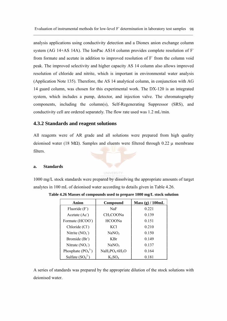
Evaluation of instrumental methods for low-level F- determination in laboratory test samples ______________________________________________________________________________________
98
analysis applications using conductivity detection and a Dionex anion exchange column
system (AG 14+AS 14A). The IonPac AS14 column provides complete resolution of F-
from formate and acetate in addition to improved resolution of F- from the column void
peak. The improved selectivity and higher capacity AS 14 column also allows improved
resolution of chloride and nitrite, which is important in environmental water analysis
(Application Note 135). Therefore, the AS 14 analytical column, in conjunction with AG
14 guard column, was chosen for this experimental work. The DX-120 is an integrated
system, which includes a pump, detector, and injection valve. The chromatography
components, including the column(s), Self-Regenerating Suppressor (SRS), and
conductivity cell are ordered separately. The flow rate used was 1.2 mL/min.
4.3.2 Standards and reagent solutions
All reagents were of AR grade and all solutions were prepared from high quality
deionised water (18 MΩ). Samples and eluents were filtered through 0.22 µ membrane
filters.
a. Standards
1000 mg/L stock standards were prepared by dissolving the appropriate amounts of target
analytes in 100 mL of deionised water according to details given in Table 4.26.
Table 4.26 Masses of compounds used to prepare 1000 mg/L stock solution
Anion Compound Mass (g) / 100mL Fluoride (F-) NaF 0.221 Acetate (Ac-) CH3COONa 0.139
Formate (HCOO-) HCOONa 0.151 Chloride (Cl-) KCl 0.210 Nitrite (NO2
-) NaNO2 0.150 Bromide (Br-) KBr 0.149 Nitrate (NO3
-) NaNO3 0.137 Phosphate (PO4
3-) NaH2PO4·6H2O 0.164 Sulfate (SO4
2-) K2SO4 0.181
A series of standards was prepared by the appropriate dilution of the stock solutions with
deionised water.
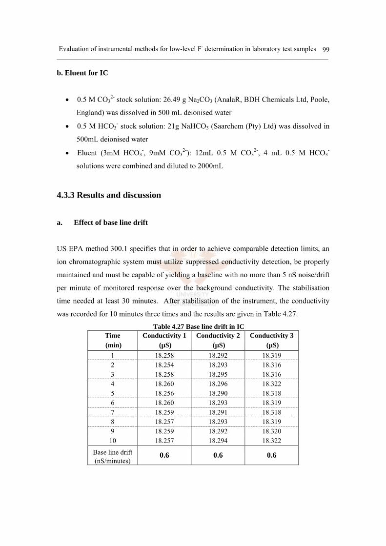
Evaluation of instrumental methods for low-level F- determination in laboratory test samples ______________________________________________________________________________________
99
b. Eluent for IC
• 0.5 M CO32- stock solution: 26.49 g Na2CO3 (AnalaR, BDH Chemicals Ltd, Poole,
England) was dissolved in 500 mL deionised water
• 0.5 M HCO3- stock solution: 21g NaHCO3 (Saarchem (Pty) Ltd) was dissolved in
500mL deionised water
• Eluent (3mM HCO3-, 9mM CO3
2-): 12mL 0.5 M CO32-, 4 mL 0.5 M HCO3
-
solutions were combined and diluted to 2000mL
4.3.3 Results and discussion
a. Effect of base line drift
US EPA method 300.1 specifies that in order to achieve comparable detection limits, an
ion chromatographic system must utilize suppressed conductivity detection, be properly
maintained and must be capable of yielding a baseline with no more than 5 nS noise/drift
per minute of monitored response over the background conductivity. The stabilisation
time needed at least 30 minutes. After stabilisation of the instrument, the conductivity
was recorded for 10 minutes three times and the results are given in Table 4.27.
Table 4.27 Base line drift in IC Time Conductivity 1 Conductivity 2 Conductivity 3 (min) (µS) (µS) (µS)
1 18.258 18.292 18.319 2 18.254 18.293 18.316 3 18.258 18.295 18.316 4 18.260 18.296 18.322 5 18.256 18.290 18.318 6 18.260 18.293 18.319 7 18.259 18.291 18.318 8 18.257 18.293 18.319 9 18.259 18.292 18.320
10 18.257 18.294 18.322
Base line drift (nS/minutes)
0.6 0.6 0.6

Evaluation of instrumental methods for low-level F- determination in laboratory test samples ______________________________________________________________________________________
100
The base line drift was calculated by the following equation:
Base line drift = 100010
H LC C−× (4.5)
Where, CH = the highest conductivity value, CL = the lowest conductivity value, 1000 is a conversion factor from µS to nS
The calculated value of the base line drift is 0.6 nS, which is acceptable.
b. Calibration study
Correct calibration is an essential factor to achieve accurate measurements of F-
concentration. Calibration lines for different standard series and the calculated linearity in
terms of correlation coefficient are presented in Table 4.28. It was found that the IC
software was set to yield the calibration function, forcing the y-intercept through zero.
Since the calibration line is normally obtained not forcing y-intercept through zero, this
table shows the calibration function and linearity using both calculation methods.
Table 4.28 Calibration factor with different set of standards
Force through zero Ignore zero Standards set Function Linearity Function Linearity
1, 5, 10 Y = 792377x 0.9996 Y = 804977x-99226 0.9999 0.05, 1, 3 Y = 198473x 0.9999 Y = 198475x-4.9656 0.9999 0.1, 0.5, 3 Y = 202925x 0.9998 Y = 204151x-3153.2 0.9999
0.05, 0.5, 3 Y = 201141x 0.9999 Y = 202093x-2481.2 1.0000 0.1, 1, 10, 50 Y = 750234x 0.9994 Y = 745853x+186479 0.9995
0.05, 0.1, 1, 5, 10 Y = 825592x 0.9989 Y = 837317x-91487 0.9994 0.05, 0.2, 0.5, 1, 3 Y = 177497x 0.9997 Y = 177708x-455.95 0.9997
A better linearity was obtained when the y-intercept was not forced through zero and
when three standards were used, rather than 4 or 5 standards. As was expected, increasing
the analytical range to include higher concentrations, such as 10 mg/L or 50 mg/L F-,
reduced the linearity. Since this study focused on low-level F- determinations, the
analytical range 0.05 to 5 mg/L was selected for further study. To evaluate the effect of
injection volume, two sample loops, 25 µL and 50 µL, were tested using a calibration

Evaluation of instrumental methods for low-level F- determination in laboratory test samples ______________________________________________________________________________________
101
standard series with concentrations 0.05, 0.2, 0.5, 2 and 5 mg/L F- and a set of spiked
samples with concentration 0.1, 0.7, 1 and 4 mg/L. The results are given in Table 4.29.
Table 4.29 Optimisation of the injection volume
25 µL loop 50 µL loop [F] Known (mg/L) [F] Measured
(mg/L) %
Recovery[F] Measured
(mg/L) %
Recovery 0.1 0.102 102.4 0.110 110.4 0.7 0.668 95.4 0.670 95.8 1 0.966 96.6 0.923 92.3 4 3.959 99.0 4.004 100.1
A better recovery was found for the lower concentration levels, 0.1, 0.7 and 1 mg/L, with
the 25 µL loop. Therefore, the 25 µL loop was used for further work.
A brand new analytical column (AS 14) was tested, with and without guard column, to
evaluate its efficiency. Usually a short guard column is placed in front of the analytical
column to increase the life of the analytical column by removing particulate matter and
contaminants from the solvents (see Section 3.2.2.d). 0.2, 0.7, 1 and 2 mg/L F- test
solutions were measured after calibration and the results are given in Table 4.30.
Table 4.30 Column efficiency on F- determination
AS 14 column Only
AG 14 + AS 14 Together [F] Known
(mg/L) [F] Measured (mg/L)
% Error
[F] Measured (mg/L)
% Error
0.2 0.184 -8.2 0.189 -5.5 0.7 0.653 -6.7 0.650 -7.1 1 0.965 -3.5 0.952 -4.8 2 1.974 -1.3 1.950 -2.5
The AS 14 analytical column, used without guard column, gave better accuracy than the
combined column system. However, to use only the analytical column for environmental
samples could reduce column life since they may contain many unknown contaminants.
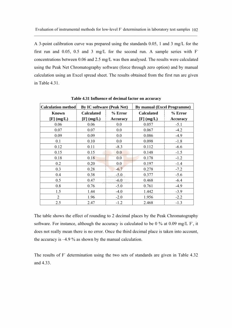
Evaluation of instrumental methods for low-level F- determination in laboratory test samples ______________________________________________________________________________________
102
A 3-point calibration curve was prepared using the standards 0.05, 1 and 3 mg/L for the
first run and 0.05, 0.5 and 3 mg/L for the second run. A sample series with F-
concentrations between 0.06 and 2.5 mg/L was then analysed. The results were calculated
using the Peak Net Chromatography software (force through zero option) and by manual
calculation using an Excel spread sheet. The results obtained from the first run are given
in Table 4.31.
Table 4.31 Influence of decimal factor on accuracy
Calculation method By IC software (Peak Net) By manual (Excel Programme) Known Calculated % Error Calculated % Error
[F] (mg/L) [F] (mg/L) Accuracy [F] (mg/L) Accuracy 0.06 0.06 0.0 0.057 -5.1 0.07 0.07 0.0 0.067 -4.2 0.09 0.09 0.0 0.086 -4.9 0.1 0.10 0.0 0.098 -1.8
0.12 0.11 -8.3 0.112 -6.6 0.15 0.15 0.0 0.148 -1.5 0.18 0.18 0.0 0.178 -1.2 0.2 0.20 0.0 0.197 -1.4 0.3 0.28 -6.7 0.278 -7.2 0.4 0.38 -5.0 0.377 -5.6 0.5 0.47 -6.0 0.468 -6.4 0.8 0.76 -5.0 0.761 -4.9 1.5 1.44 -4.0 1.442 -3.9 2 1.96 -2.0 1.956 -2.2
2.5 2.47 -1.2 2.468 -1.3
The table shows the effect of rounding to 2 decimal places by the Peak Chromatography
software. For instance, although the accuracy is calculated to be 0 % at 0.09 mg/L F-, it
does not really mean there is no error. Once the third decimal place is taken into account,
the accuracy is –4.9 % as shown by the manual calculation.
The results of F- determination using the two sets of standards are given in Table 4.32
and 4.33.
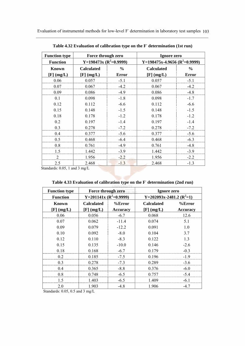
Evaluation of instrumental methods for low-level F- determination in laboratory test samples ______________________________________________________________________________________
103
Table 4.32 Evaluation of calibration type on the F- determination (1st run)
Function type Force through zero Ignore zero Function Y=198473x (R2=0.9999) Y=198475x-4.9656 (R2=0.9999) Known Calculated % Calculated %
[F] (mg/L) [F] (mg/L) Error [F] (mg/L) Error 0.06 0.057 -5.1 0.057 -5.1 0.07 0.067 -4.2 0.067 -4.2 0.09 0.086 -4.9 0.086 -4.8 0.1 0.098 -1.8 0.098 -1.7 0.12 0.112 -6.6 0.112 -6.6 0.15 0.148 -1.5 0.148 -1.5 0.18 0.178 -1.2 0.178 -1.2 0.2 0.197 -1.4 0.197 -1.4 0.3 0.278 -7.2 0.278 -7.2 0.4 0.377 -5.6 0.377 -5.6 0.5 0.468 -6.4 0.468 -6.3 0.8 0.761 -4.9 0.761 -4.8 1.5 1.442 -3.9 1.442 -3.9 2 1.956 -2.2 1.956 -2.2
2.5 2.468 -1.3 2.468 -1.3 Standards: 0.05, 1 and 3 mg/L
Table 4.33 Evaluation of calibration type on the F- determination (2nd run)
Function type Force through zero Ignore zero Function Y=201141x (R2=0.9999) Y=202093x-2481.2 (R2=1) Known Calculated %Error Calculated %Error
[F] (mg/L) [F] (mg/L) Accuracy [F] (mg/L) Accuracy 0.06 0.056 -6.7 0.068 12.6 0.07 0.062 -11.4 0.074 5.1 0.09 0.079 -12.2 0.091 1.0 0.10 0.092 -8.0 0.104 3.7 0.12 0.110 -8.3 0.122 1.3 0.15 0.135 -10.0 0.146 -2.6 0.18 0.168 -6.7 0.179 -0.3 0.2 0.185 -7.5 0.196 -1.9 0.3 0.278 -7.3 0.289 -3.6 0.4 0.365 -8.8 0.376 -6.0 0.8 0.748 -6.5 0.757 -5.4 1.5 1.403 -6.5 1.409 -6.1 2.0 1.903 -4.8 1.906 -4.7
Standards: 0.05, 0.5 and 3 mg/L
Evaluation of instrumental methods for low-level F- determination in laboratory test samples ______________________________________________________________________________________
104
For the first run, the concentration values were accurate but not for the second run where
concentrations were underestimated when calculated using a “force through zero”
calibration line. The calibration line, which ignored zero, gave acceptable results for the
second run. In the case of first run, the results for both calibration lines were good. In this
case, the y-intercept of the calibration function was only –4.9656 and close to zero.
Therefore, even after forcing the y-intercept through zero, the function was not changed
much. However, for the second run, the y-intercept was –2481.2, which was a quite big
value. Thus, when the y-intercept was forced through zero, the linearity of calibration line
was reduced and low concentrations, especially, show large errors.
These results indicate that establishing a proper calibration function is of utmost
importance, for achieving an accurate F- determination. Therefore, every effort must be
made to establish the best calibration line possible. Experimental aspects to consider
include using very accurate and properly calibrated volumetric equipment such as
pipettes, clean containers, and correctly prepared standards. If the calibration line is well
established like the first run in Table 4.38, very accurate results can be obtained.
On the other hand, when calibration line is not well established like second run, then the
appropriate choice of calibration function, for example ignoring zero on the calibration
line, becomes important. It was found that peak threshold value could affect the F-
determination. The threshold is a value derived from the averaged slopes of data bunches
along a baseline sector. It is applied as a limiting slope to determine peaks. It marks the
potential start of a peak when two consecutive data bunches have a slope higher than the
peak threshold value (Dionex, 1997). Several values of peak threshold were tested to
optimise the best value for accurate F- determination. It is given in Table 4.34.

Evaluation of instrumental methods for low-level F- determination in laboratory test samples ______________________________________________________________________________________
105
Table 4.34 Optimisation of peak threshold
Threshold 1 0.5 0.12 0.06 [F] (mg/L) [F] (mg/L) [F] (mg/L) [F] (mg/L) [F] (mg/L)
Known Measured %
Error Measured%
Error Measured%
Error Measured %
Error0.3 0.25 -16.7 0.25 -16.7 0.3 0.0 0.32 6.7 0.7 0.65 -7.1 0.65 -7.1 0.68 -2.9 0.7 0.0 2 1.92 -4.0 1.94 -3.0 1.99 -0.5 1.98 -1.0
Threshold 0.03 0.01 0.0025 0.001 [F] (mg/L) [F] (mg/L) [F] (mg/L) [F] (mg/L) [F] (mg/L)
Known Measured %
Error Measured%
Error Measured%
Error Measured %
Error0.3 0.32 6.7 0.30 0.0 0.30 0.0 0.30 0.0 0.7 0.70 -0.4 0.66 -5.7 0.66 -5.7 0.66 -5.7 2 1.98 -0.8 1.94 -3.0 1.94 -3.0 1.94 -3.0
0.3, 0.7 and 2 mg/L F- test solutions were examined with various peak threshold values
and this table shows that the results were varying according to the peak threshold value.
The results obtained using the peak threshold value 1 and 0.5 are very similar and also
between 0.12 and 0.03. The results obtained using the peak threshold value 0.01, 0.0025
and 0.001 are exactly same, but the best value in this table is 0.12. It is reasonable to use
the peak threshold between 0.12 and 0.03 but 0.12 is recommended.
c. Interference study
IonPac AS4A, recommended in US EPA 300.0 (1993), is appropriate for the analysis of
anions in low ionic strength, well-characterized samples, such as drinking and surface
waters. However, this column is not recommended for the analysis of F- in more complex
samples, e.g. containing organic acids, such as acetate and formate. However, the AS 14
column provides improved F- resolution from the system void peak and complete
resolution of F- from formate and/or acetate (Application Note 133; Jackson, 2001). The
improved selectivity, along with higher capacity, makes the AS 14 column a better choice
for higher ionic strength water samples and more complex matrices, such as domestic and
industrial wastewaters.
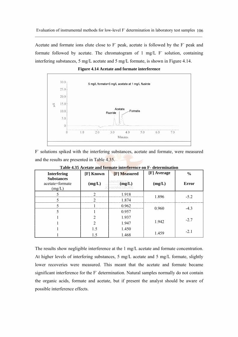
Evaluation of instrumental methods for low-level F- determination in laboratory test samples ______________________________________________________________________________________
106
Acetate and formate ions elute close to F- peak, acetate is followed by the F- peak and
formate followed by acetate. The chromatogram of 1 mg/L F- solution, containing
interfering substances, 5 mg/L acetate and 5 mg/L formate, is shown in Figure 4.14.
Figure 4.14 Acetate and formate interference
F- solutions spiked with the interfering substances, acetate and formate, were measured
and the results are presented in Table 4.35.
Table 4.35 Acetate and formate interference on F- determination Interfering [F] Known [F] Measured [F] Average % Substances
acetate+formate (mg/L)
(mg/L) (mg/L) (mg/L) Error
5 2 1.918 5 2 1.874
1.896 -5.2
5 1 0.962 5 1 0.957
0.960 -4.3
1 2 1.937 1 2 1.947
1.942 -2.7
1 1.5 1.450 1 1.5 1.468
1.459 -2.1
The results show negligible interference at the 1 mg/L acetate and formate concentration.
At higher levels of interfering substances, 5 mg/L acetate and 5 mg/L formate, slightly
lower recoveries were measured. This meant that the acetate and formate became
significant interference for the F- determination. Natural samples normally do not contain
the organic acids, formate and acetate, but if present the analyst should be aware of
possible interference effects.

Evaluation of instrumental methods for low-level F- determination in laboratory test samples ______________________________________________________________________________________
107
d. Analytical parameters
The definition of each analytical parameter, given below, is given in Section 4.2.3.e.
i) Repeatability
To determine repeatability, 0.2, 0.3, 0.7, 1.0 and 2.0 mg/L F test solutions were measured
10 times each. The results are given in Table 4.36 and the repeatability was expressed in
terms of % RSD.
Table 4.36 The repeatability of IC
[F] Conc. Mean intensity % RSD (mg/L) (µS)
SD (N=10) (Repeatability)
0.2 40541.8 2264.9 5.6 0.3 57566.5 2049.4 3.6 0.7 132797.4 1747.2 1.3 1.0 188935.9 2910.4 1.5 2.0 388150.6 2754.2 0.7
As the concentration increases, the repeatability becomes better, as was expected. This
phenomenon was also observed in the ISE measurements. The repeatability in the case of
ISE, given in Table 4.32, was 0.2 % and 0.3 % at 1 mg/L and 2 mg/L, respectively. These
values are significantly better than the values found for the IC method.
ii) Method Detection Limit (MDL)
MDL could not be determined using the procedure based on 3x the standard deviation of
several blank measurements, because in IC a blank sample results in no peak and thus
cannot be integrated. Therefore, alternative procedures for the determination of detection
limit were investigated.
In the first procedure a calibration curve was derived from a set of successively diluted
standards and the detection limits obtained experimentally. The qualitative detection limit
for F- was taken as the lowest concentration at which a peak could be distinguished from
the background. This was 0.05 mg/L. The quantitative detection limit was determined as
the lowest concentration of F- needed to produce a peak that could be integrated and
plotted on a linear calibration curve. The quantitative detection limit was determined as
0.03 mg/L.
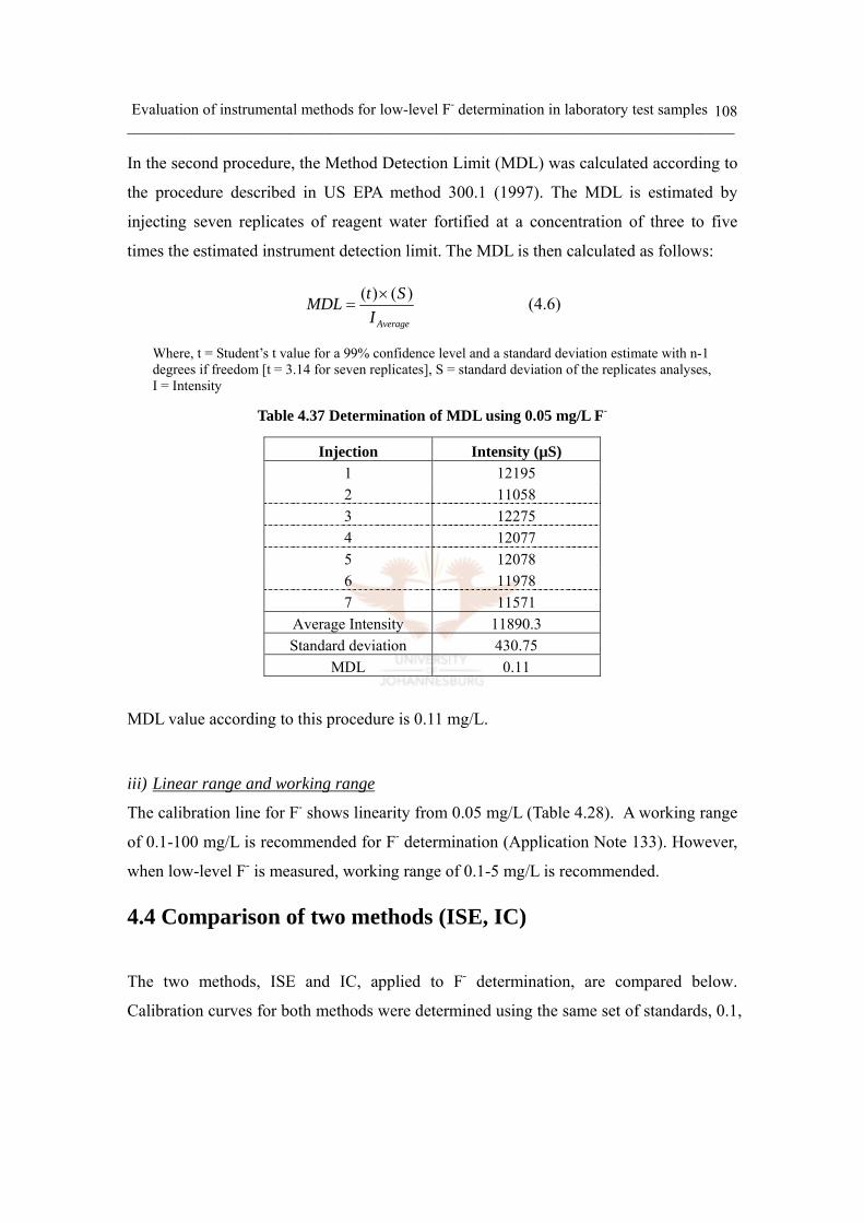
Evaluation of instrumental methods for low-level F- determination in laboratory test samples ______________________________________________________________________________________
108
In the second procedure, the Method Detection Limit (MDL) was calculated according to
the procedure described in US EPA method 300.1 (1997). The MDL is estimated by
injecting seven replicates of reagent water fortified at a concentration of three to five
times the estimated instrument detection limit. The MDL is then calculated as follows:
( ) ( )
Average
t SMDLI×
= (4.6)
Where, t = Student’s t value for a 99% confidence level and a standard deviation estimate with n-1 degrees if freedom [t = 3.14 for seven replicates], S = standard deviation of the replicates analyses, I = Intensity
Table 4.37 Determination of MDL using 0.05 mg/L F-
Injection Intensity (µS) 1 12195 2 11058 3 12275 4 12077 5 12078 6 11978 7 11571
Average Intensity 11890.3 Standard deviation 430.75
MDL 0.11
MDL value according to this procedure is 0.11 mg/L.
iii) Linear range and working range
The calibration line for F- shows linearity from 0.05 mg/L (Table 4.28). A working range
of 0.1-100 mg/L is recommended for F- determination (Application Note 133). However,
when low-level F- is measured, working range of 0.1-5 mg/L is recommended.
4.4 Comparison of two methods (ISE, IC)
The two methods, ISE and IC, applied to F- determination, are compared below.
Calibration curves for both methods were determined using the same set of standards, 0.1,
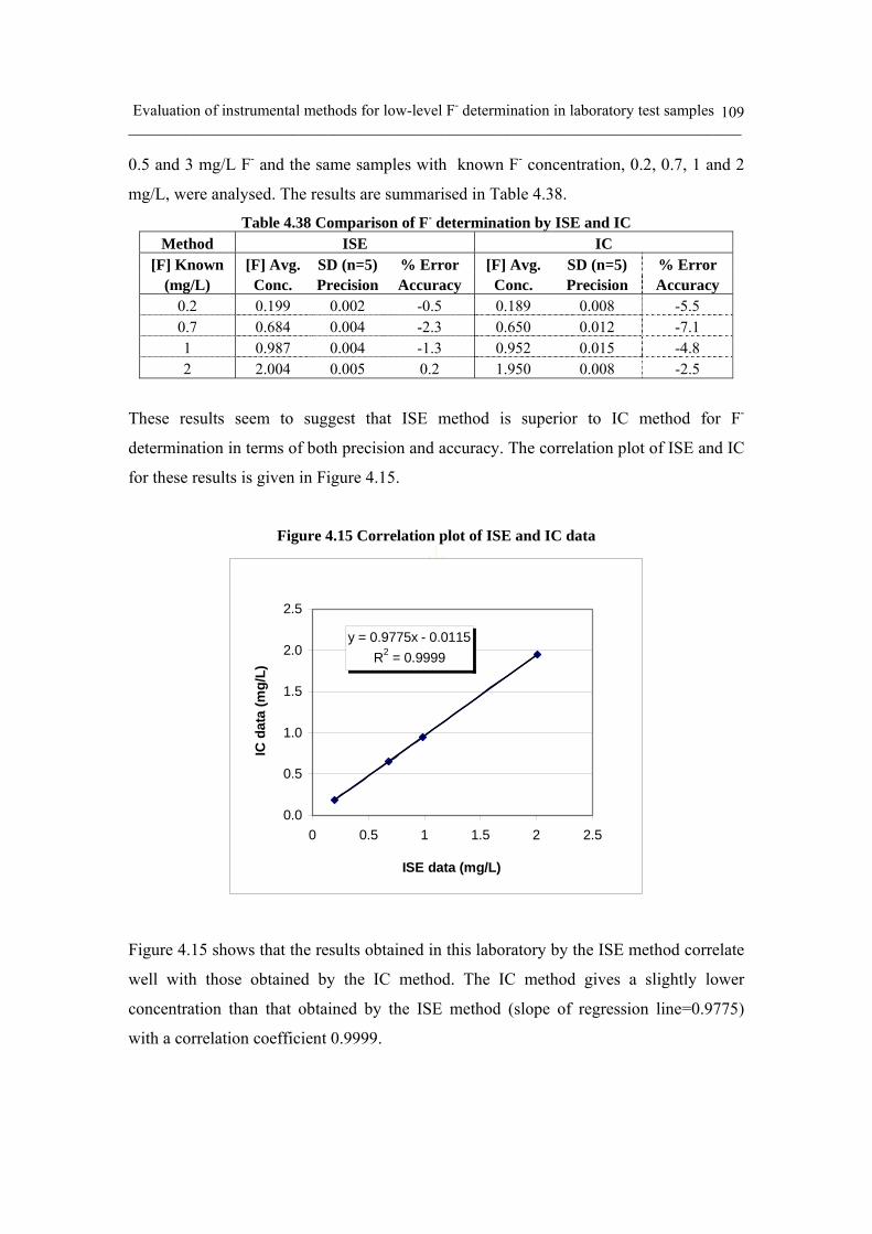
Evaluation of instrumental methods for low-level F- determination in laboratory test samples ______________________________________________________________________________________
109
0.5 and 3 mg/L F- and the same samples with known F- concentration, 0.2, 0.7, 1 and 2
mg/L, were analysed. The results are summarised in Table 4.38.
Table 4.38 Comparison of F- determination by ISE and IC Method ISE IC
[F] Known [F] Avg. SD (n=5) % Error [F] Avg. SD (n=5) % Error (mg/L) Conc. Precision Accuracy Conc. Precision Accuracy
0.2 0.199 0.002 -0.5 0.189 0.008 -5.5 0.7 0.684 0.004 -2.3 0.650 0.012 -7.1 1 0.987 0.004 -1.3 0.952 0.015 -4.8 2 2.004 0.005 0.2 1.950 0.008 -2.5
These results seem to suggest that ISE method is superior to IC method for F-
determination in terms of both precision and accuracy. The correlation plot of ISE and IC
for these results is given in Figure 4.15.
Figure 4.15 Correlation plot of ISE and IC data
y = 0.9775x - 0.0115R2 = 0.9999
0.0
0.5
1.0
1.5
2.0
2.5
0 0.5 1 1.5 2 2.5
ISE data (mg/L)
IC d
ata
(mg/
L)
Figure 4.15 shows that the results obtained in this laboratory by the ISE method correlate
well with those obtained by the IC method. The IC method gives a slightly lower
concentration than that obtained by the ISE method (slope of regression line=0.9775)
with a correlation coefficient 0.9999.
Evaluation of instrumental methods for low-level F- determination in laboratory test samples ______________________________________________________________________________________
110
4.5 Methodology recommendations
4.5.1 ISE ISE is a simple and accurate method for low level F- determination. Electrode drift is one
of the main problems, especially at low concentrations. To minimise the electrode drift
and improve the equilibrium time, F- ion selective electrodes are recommended to be
stored dry in air and the reference electrode in deionised water. Cleaning the electrode
regularly with F- toothpaste is a very effective way to minimize the electrode drift as well
as improve the linearity of electrode response. It is recommended to use low level
standards, such as 0.1, 1 and 3 mg/L, for low level determination. TISAB is normally
added to samples and standards in ISE measurement in order to maintain a constant ionic
strength for both standards and samples, optimise the pH, and de-complex interference
ions. Low Level TISAB and TISAB III are available for low-level measurement, but
TISAB III is recommended in natural samples, which contain many unknown
interferences. Since Low Level TISAB does not contain de-complexation agent, such as
CDTA, it can not be used in natural samples. Most ionic interferences, except the Al ion,
which readily form stable complexes with F- ions, can be removed by using TISAB III.
The Al tolerance for 95 % F- recovery is 0.2 mg/L and 0.1 mg/L for 1 mg/L F- and 0.2
mg/L F- , respectively. Tri-ammonium citrate (TAC) buffer, can improve the Al tolerance
up to 5 mg/L for 94% F- recovery, and is recommended in presence of high
concentrations of Al. However, TISAB III can be applied for most of natural samples
since the Al level is mostly below 0.2 mg/L. Synergistic effects in ISE have been
demonstrated when many interfering substances are present.
4.5.2 IC It is necessary to allow stabilisation time on the IC instrument of at least 30 minutes. IC
base line drift, determined experimentally, was 0.6 nS/minute, which was acceptable. A
3-point calibration at low concentrations, such as 0.1, 1 and 3 mg/L, is recommended. A
25 µL injection volume yielded better results than a 50 µL sample loop. The optimised
peak threshold value was 0.12. IC software calculates the calibration function by forcing
Evaluation of instrumental methods for low-level F- determination in laboratory test samples ______________________________________________________________________________________
111
the y-intercept through zero. Because of this fact, it is essential to have proper calibration
line where the y-intercept is close to zero. If not, manual calibration line calculation must
be performed. 5 minutes run time is enough to analyse the samples for F- or even acetate
and formate, since these ions are also eluted within 5 minutes. Possible interference on IC
is co-elution of organic acid anions, such as acetate and formate. The interference of 1
mg/L acetate together with 1 mg/L formate was not significant. The IC method is
appropriate for the analysis of anions in low ionic strength, well-characterized samples,
such as drinking and surface waters, since natural water samples normally do not contain
formate and acetate.
4.6 Conclusion
Method validation and the development of standard ISE and IC procedures for the
accurate determination of low-level F-, was conducted. Although the results, obtained by
the ISE and IC, produced a good correlation, ISE gave more accurate and precise results.
As mentioned in Chapter 1, the accuracy of the F- determination is a very important
aspect in terms of fluoridation. Therefore, ISE is recommended for low-level F-
determination.

Comparison of IC and ISE for the analysis of natural and drinking water ______________________________________________________________________________________
112
Chapter 5
Comparison of IC and ISE for the analysis of natural and drinking water
5.1 Introduction
Chapter 4 focused on the evaluation of the ISE and IC methods for the determination of
F-. A detailed study of calibration and measurement procedures and ways of dealing with
matrix interferences have been carried out to ensure that the best possible analytical
methodologies are followed throughout this study. In Chapter 5 the methodologies
developed in Chapter 4 are applied to the analysis of natural waters such as river water
(Vaal and Crocodile rivers), dam water (Hartbeespoort Dam), and drinking water
(Johannesburg municipal tap water). The main objective was to evaluate the performance
of the chosen methods in the analysis of real samples and to assess the effect of the
sample matrix on the accuracy of F- determinations.
5.2 Laboratory Fortified sample Matrix (LFM) A useful procedure to assess whether a method is prone to matrix effects, is the
laboratory fortified sample matrix method, which is a quality control procedure used in
the EPA approved method for F- determination (EPA Method 300.1, Daniel P.H., 1997).
The Laboratory Fortified sample Matrix (LFM) is an aliquot of an environmental sample
to which known quantities of the method analytes are added in the laboratory. The LFM
is analyzed exactly like a sample, and its purpose is to determine whether the sample
matrix contributes bias to the analytical results. The background concentrations of the
analytes in the sample matrix must be determined in a separate aliquot and the measured
values in the LFM corrected for background concentrations. The LFM should be
prepared at concentrations no greater than five times the highest concentration observed
in any field sample.
Comparison of IC and ISE for the analysis of natural and drinking water ______________________________________________________________________________________
113
Percent Recovery is calculated using the following equation:
R = 100×−S
CCs (5.1)
Where, R = % recovery, Cs = fortified sample concentration, C = sample background concentration, S = concentration equivalent of analyte added to sample
According to the U.S. EAP method 300.1, the recovery limit ranges are from 75 to 125%.
If the recovery of any analyte falls outside the designated LFM recovery range, the
recovery problem encountered with the LFM is judged to be matrix induced and the
results for that sample and the LFM are reported with a “matrix induced bias” qualifier.
5.3 Experimental 5.3.1 Instrumentation a. ISE
An ORION 940 auto chemistry system, equipped with a 9404 sc ORION F- electrode
connected to an Ag/AgCl Model 90-01 single junction reference electrode, was used for
the measurement of F- in each sample. TISAB III (Orion) was used as a Total Ionic
Strength Adjustment Buffer.
b. IC
A Dionex DX-120 Ion Chromatographic system, equipped with a Dionex anion exchange
column system (AG 14A+AS14A), was used for the determination of F- in each sample.
The Standard HCO3-/CO3
2- (1.0 mM HCO3- + 3.5mM CO3
2-) eluent, recommended for
anion determinations with this column, was used in IC measurement. All the samples and
eluent were filtered through 0.22 µm membrane filters, prior to analysis.
c. ICP-OES
ICP-OES was used to determine the cation elemental composition in tap water. Multi-
element calibration was used for the determination of the elements: Li, B, Na, Mg, Al, Ca,
Cr, Mn, Fe, Co, Ni, Cu, Zn, Sr, Ba, Cd, Pb and Bi using a Varian Liberty 110 ICP

Comparison of IC and ISE for the analysis of natural and drinking water ______________________________________________________________________________________
114
Emission spectrometer. A 1000 mg/L ICP multi-element standard solution IV (Merck)
was used to prepare calibration standards by appropriate dilution with 2% HNO3. The
experimental conditions used in ICP-OES measurements are summarized in Table 5.1.
Table 5.1 ICP-OES operational conditions of multi-element determination
Parameter Setting
Viewing Height 6 mm
Search window 0.04 nm
Generator power 1.20 kW
Plasma gas flow rate 15.0 L/min
Auxiliary gas flow rate 1.50 L/min
Pump speed 25.0 rpm
d. ICP-MS
Inductively coupled plasma mass spectrometry (ICP-MS) was used to determine the
cation elemental composition in the Crocodile and Vaal rivers and Hartbeesport Dam
water matrices. Multi-element calibration was also used for the determination of the
elements: Na, Mg, Al, Si, K, Ti, V, Cr, Mn, Fe, Ni, Zn, Cu, Ga, As, Se, Sr, Rh, Cd, Sb
and Pb using a X Series ICP-MS spectrometer (Thermo Elemental). A 1000 mg/L ICP
multi-element standard solution IV (Merck) was used to prepare calibration standards by
appropriate dilution with 2% HNO3.
5.3.2 Reagents, standard solutions and sample preparation
All reagents were of AR grade and high quality deionised water (18 MΩ) was used for
preparing all solutions. Samples and eluents were filtered through 0.22 µm membrane
filters.
The following solutions were prepared:
• 1000 mg/L F- Stock solution: 0.221 g NaF was dissolved in deionised water and
diluted to 100 ml in a polystyrene volumetric flask.
• TISAB lll (Thermo Orion, Cat. No. 940911)
• Single Junction Reference Electrode Filling solution (contents 60 ml, 900001)
Comparison of IC and ISE for the analysis of natural and drinking water ______________________________________________________________________________________
115
• 0.5 M CO32- stock solution: 26.49 g Na2CO3 (AnalaR, BDH Chemicals Ltd, Poole,
England) was dissolved in 500 ml deionised water.
• 0.5 M HCO3- stock solution: 21.00 g NaHCO3 (Saarchem(Pty)Ltd) was dissolved
in 500 ml deionised water.
• Eluent (3.5 mM CO32-, 1.0 mM HCO3
-): 12 ml 0.5 M CO32- and 4 ml 0.5 M HCO3
-
solutions were combined and diluted to 2000 ml.
• 1000 mg/L ICP Multi-element standard solution IV (Merck)
• LFM samples: The filtered natural water samples were spiked with appropriate
amounts of NaF to obtain a series of LFM samples for each of the sample types,
containing 0.1, 0.2, 0.5 and 1 mg/L F-.
5.3.3 Experimental procedure
The methods, ISE and IC, were used for the determination of F- concentrations in the
fortified samples. The background F- concentration was determined in the unspiked
sample. Calibration Check Standards (CCS) were measured as recommended in the U.S.
EPA method 300.1. The 3 different kinds of CCS were:
• Initial calibration check standard: It verified the previously established calibration
curve.
• Continuing calibration check standard: It confirmed accurate analyte quantitation
for the previous samples analyzed. It should be measured in every tenth sample
measurement.
• End calibration check standard: It verified the previously established calibration
curve and confirmed accurate analyte quantitation for all the samples since the last
one.
a. ISE
2 ml of TISAB III was added to the 20 ml of test and standard solutions, as recommended
in the manufacturer’s procedure (TISAB III : sample volume = 1:10 for the determination
of F-).
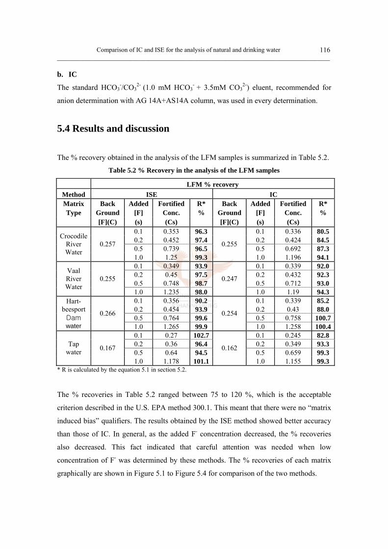
Comparison of IC and ISE for the analysis of natural and drinking water ______________________________________________________________________________________
116
b. IC
The standard HCO3-/CO3
2- (1.0 mM HCO3- + 3.5mM CO3
2-) eluent, recommended for
anion determination with AG 14A+AS14A column, was used in every determination.
5.4 Results and discussion
The % recovery obtained in the analysis of the LFM samples is summarized in Table 5.2.
Table 5.2 % Recovery in the analysis of the LFM samples
LFM % recovery Method ISE IC Matrix Back Added Fortified R* Back Added Fortified R* Type Ground [F] Conc. % Ground [F] Conc. %
[F](C) (s) (Cs) [F](C) (s) (Cs) 0.1 0.353 96.3 0.1 0.336 80.50.2 0.452 97.4 0.2 0.424 84.50.5 0.739 96.5 0.5 0.692 87.3
Crocodile River Water
0.257
1.0 1.25 99.3
0.255
1.0 1.196 94.10.1 0.349 93.9 0.1 0.339 92.00.2 0.45 97.5 0.2 0.432 92.30.5 0.748 98.7 0.5 0.712 93.0
Vaal River Water
0.255
1.0 1.235 98.0
0.247
1.0 1.19 94.30.1 0.356 90.2 0.1 0.339 85.20.2 0.454 93.9 0.2 0.43 88.00.5 0.764 99.6 0.5 0.758 100.7
Hart- beesport Dam water
0.266
1.0 1.265 99.9
0.254
1.0 1.258 100.40.1 0.27 102.7 0.1 0.245 82.80.2 0.36 96.4 0.2 0.349 93.30.5 0.64 94.5 0.5 0.659 99.3
Tap water 0.167
1.0 1.178 101.1
0.162
1.0 1.155 99.3* R is calculated by the equation 5.1 in section 5.2.
The % recoveries in Table 5.2 ranged between 75 to 120 %, which is the acceptable
criterion described in the U.S. EPA method 300.1. This meant that there were no “matrix
induced bias” qualifiers. The results obtained by the ISE method showed better accuracy
than those of IC. In general, as the added F- concentration decreased, the % recoveries
also decreased. This fact indicated that careful attention was needed when low
concentration of F- was determined by these methods. The % recoveries of each matrix
graphically are shown in Figure 5.1 to Figure 5.4 for comparison of the two methods.

Comparison of IC and ISE for the analysis of natural and drinking water ______________________________________________________________________________________
117
Figure 5.1 Method comparison of the LFM % Recovery in Crocodile River
0
20
40
60
80
100
120
0.1 0.2 0.5 1Added [F] (mg/l)
LFM
% R
ecov
ery
ISE IC
Figure 5.2 Method comparison of the LFM % Recovery in Vaal River
020406080
100120
0.1 0.2 0.5 1
Added [F] (mg/l)
LFM
% R
ecov
ery
ISE IC
Figure 5.3 Method comparison of the LFM % Recovery in Hartbeespoort Dam
020406080
100120
0.1 0.2 0.5 1Added [F] (mg/l)
LFM
% R
ecov
ery
ISE IC
Figure 5.4 Method comparison of the LFM % Recovery in Tap water
0
2 0
4 0
6 0
8 0
1 0 0
1 2 0
0 .1 0 .2 0 .5 1A d d e d [ F ] (m g /l )
LFM
% R
ecov
ery
IS E IC
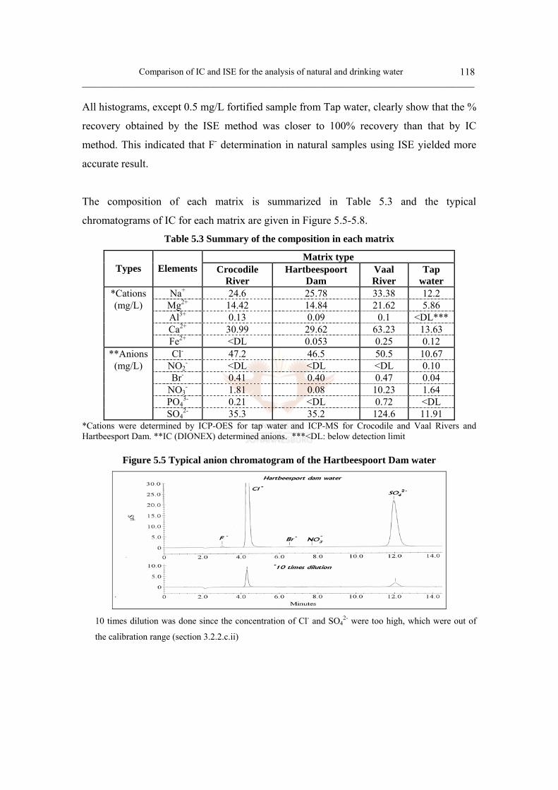
Comparison of IC and ISE for the analysis of natural and drinking water ______________________________________________________________________________________
118
All histograms, except 0.5 mg/L fortified sample from Tap water, clearly show that the %
recovery obtained by the ISE method was closer to 100% recovery than that by IC
method. This indicated that F- determination in natural samples using ISE yielded more
accurate result.
The composition of each matrix is summarized in Table 5.3 and the typical
chromatograms of IC for each matrix are given in Figure 5.5-5.8.
Table 5.3 Summary of the composition in each matrix
Matrix type Types Elements Crocodile
River Hartbeespoort
Dam Vaal River
Tap water
*Cations Na+ 24.6 25.78 33.38 12.2 (mg/L) Mg2+ 14.42 14.84 21.62 5.86
Al3+ 0.13 0.09 0.1 <DL*** Ca2+ 30.99 29.62 63.23 13.63 Fe2+ <DL 0.053 0.25 0.12
**Anions Cl- 47.2 46.5 50.5 10.67 (mg/L) NO2
- <DL <DL <DL 0.10 Br- 0.41 0.40 0.47 0.04 NO3
- 1.81 0.08 10.23 1.64 PO4
3- 0.21 <DL 0.72 <DL SO4
2- 35.3 35.2 124.6 11.91 *Cations were determined by ICP-OES for tap water and ICP-MS for Crocodile and Vaal Rivers and Hartbeesport Dam. **IC (DIONEX) determined anions. ***<DL: below detection limit
Figure 5.5 Typical anion chromatogram of the Hartbeespoort Dam water
10 times dilution was done since the concentration of Cl- and SO4
2- were too high, which were out of
the calibration range (section 3.2.2.c.ii)
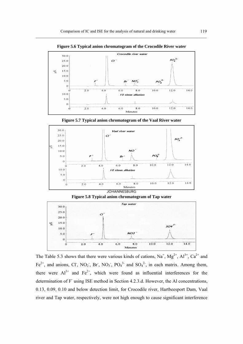
Comparison of IC and ISE for the analysis of natural and drinking water ______________________________________________________________________________________
119
Figure 5.6 Typical anion chromatogram of the Crocodile River water
Figure 5.7 Typical anion chromatogram of the Vaal River water
Figure 5.8 Typical anion chromatogram of Tap water
The Table 5.3 shows that there were various kinds of cations, Na+, Mg2+, Al3+, Ca2+ and
Fe2+, and anions, Cl-, NO2-, Br-, NO3
-, PO43- and SO4
2-, in each matrix. Among them,
there were Al3+ and Fe2+, which were found as influential interferences for the
determination of F- using ISE method in Section 4.2.3.d. However, the Al concentrations,
0.13, 0.09, 0.10 and below detection limit, for Crocodile river, Hartbeesport Dam, Vaal
river and Tap water, respectively, were not high enough to cause significant interference

Comparison of IC and ISE for the analysis of natural and drinking water ______________________________________________________________________________________
120
in the measurement of F- using ISE. Similarly, the Fe concentrations, below detection
limit, 0.053, 0.25 and 0.12, for Crocodile River, Hartbeesport Dam, Vaal River and Tap
water, respectively, were also not expected to cause significant interference. Therefore
the % recoveries, obtained by ISE method, were very good.
Compared to the results obtained by ISE, IC results showed an underestimation of F-
concentration. As described in Section 4.3.3.c, the underestimated results from IC
measurement could be explained in terms of interfering anions, such as the formate and
acetate anions, eluting close to the F- peak. However, there was no significant
interference from formate and acetate in each matrix in Table 5.3 and Figure 5.5-5.8.
Another possible reason could be Al interference. According to the description in Table
4.19, a 100% F- recovery could not be obtained in the presence of Al, if the concentration
was more than 0.2 mg/L, even using TISAB III that contained a decomplexing agent such
as CDTA. Since there was no decomplexing agent in the IC eluent, underestimated
results could be expected. However, it was found that no Al-F complex forms at pH 9 (IC
conditions) with the less than 19 mg/L F- and 1 mg/L or 10 mg/L Al according to the
theoretical distribution curve for the species in the Al-F-OH system calculated using the
computer programme Species-Calc (Prof Hans Rohwer, Mandela Metropolitan
University of Port Elizabeth) and shown in Figure 5.9 and Figure 5.10.
Figure 5.9 Distribution curves for Al-F-OH system
Where, the values of x-axis, 1=190000mg/L, 0=19000 mg/L, -2=190mg/L, -4=1.9 mg/L F-
[Al] = 10 mg/L at pH 9

Comparison of IC and ISE for the analysis of natural and drinking water ______________________________________________________________________________________
121
Figure 5.10 Distribution curves for Al-F-OH system
Where, [Al] = 1 mg/L at pH 9
These diagrams show a very similar shape at 1 mg/L and 10 mg/L Al and were assumed
to be also valid at 0.2 mg/L Al which was the approximate background concentration of
each matrix, 0.257, 0.255, 0.266 and 0.17 in Crocodile River, Hartbeesport Dam, Vaal
River and Tap water, respectively. This meant that Al could not be the reason for the
underestimated value of F- determination using IC method.
The comparison study of two methods ISE and IC, on laboratory deionised water matrix
in Section 4.4, showed that the accuracy of IC method for F- determination at low level,
was poor. The values of accuracy at 0.2 mg/L and 0.7 mg/L were –5.5 % and –7.1 %,
respectively. When the IC method was applied to the natural sample matrix, the accuracy
at low level, such as 0.3 mg/L and 0.4 mg/L after fortification, became worse (see Table
5.2). This meant that the IC method for F- determination seemed to be more prone to the
influence of the matrix than the ISE method at low concentration levels.
5.5 Conclusion
The evaluation of the ISE and IC methods for the determination of F- in a deionised water
matrix was investigated in Chapter 4. In Chapter 5, the methodologies developed in
Chapter 4 were applied to the analysis of natural waters such as river water (Vaal and
Comparison of IC and ISE for the analysis of natural and drinking water ______________________________________________________________________________________
122
Crocodile Rivers), Dam water (Hartbeespoort Dam), and drinking water (Johannesburg
municipal tap water). The performance of two methods, ISE and IC, in the analysis of
real samples, was investigated by analysing LFM samples. The % recoveries of all LFM
samples were within the acceptable range, which was between 75 to 120 % given in the
U.S. EPA method 300.1. All the values, except the 0.5 mg/L fortified sample from Tap
water, in Table 5.2, clearly show that the % recovery obtained by the ISE method was
closer to 100% recovery than that by the IC, which meant ISE method in natural sample
yielded a more accurate result. The IC method seemed to be more affected by the
influence of the matrix. ISE methodology was found to be preferable for the accurate
determination of F- in natural water sample matrices as well as a deionised water matrix
as was concluded in Chapter 4.

Inter-laboratory study (SABS water-check proficiency testing programme) ______________________________________________________________________________
123
Chapter 6
Inter-laboratory study (SABS water-check proficiency testing programme)
6.1 Introduction
The South African Bureau of Standards (SABS), Test House runs an ongoing Water
Check Programme. Water-Check is a high frequency inter-laboratory proficiency testing
programme with the objective of providing a rapid report-back service to participants for
self evaluation. Participation in the scheme was an important part of this study because it
provided the opportunity to obtain information about the current status of fluoride (F-)
determination in South African laboratories. The SABS was also requested to include
additional F- containing solutions, specially designed to test possible matrix effects
during F- determination. This provided invaluable data and proved to be very useful in
formulating the final recommendations and conclusions. Participation in this scheme was
therefore done for the following reasons:
i) To have the opportunity for the inclusion of special samples in the Water Check
programme to test the response of different analytical methods for
F- determination to matrices containing known interfering elements such as Al
ii) To evaluate the proficiency of South African analytical laboratories for
F- determination
iii) To explain trends in the results in terms of analytical pitfalls in F- determination
and to make recommendations for accurate F- determinations
iv) To check proficiency of the procedures developed in this study
The determination of F- was included in this study, because F- was the target element in
the public water fluoridation programme envisaged for South Africa. It was important to
investigate the chemistry and analytical chemistry of F- before implementation of the
fluoridation.

Inter-laboratory study (SABS water-check proficiency testing programme) ______________________________________________________________________________
124
6.1.1 Programme design The programme is divided into three categories, each category being scheduled on a
quarterly basis. Real, spiked and /or synthetic samples are prepared for each study.
Table 6.1 SABS water-check proficiency testing programme design Group number Determinants Scheduled
1
Heavy metals in water: aluminium, barium, beryllium, boron, cadmium, chromium, cobalt, copper, iron, lead, manganese, molybdenum, nickel, silicon, strontium, vanadium, zinc, mercury, arsenic and selenium.
January April July
October
2
Nutrients and oxygen demand: nitrogen, nitrate, ammonia, total phosphate, orthophosphate, oxygen absorbed , chemical oxygen demand: dissolved organic carbon and total organic carbon
February May
August November
3
Major constituents in water: pH, conductivity, dissolved solids, calcium, magnesium, sodium, potassium, chloride, fluoride, sulphate, alkalinity, turbidity and nitrate
March June
SeptemberDecember
The programme structure therefore allows a laboratory to choose participation in one, two
or all three groups. All participants are coded for confidentiality purposes.
6.2 Major constituents in water: (Group 3) Participation in Group 3 of the March 2004 Water Check programme was scheduled for
the purposes of this MSc study. The Group 3 programme consists of the analysis of river,
borehole water and synthetic water samples. This group covers the analysis of pH,
conductivity, dissolved solids, calcium, magnesium, sodium, potassium, chloride, sulfate,
alkalinity, fluoride, nitrate and turbidity.
6.2.1 Samples for the Group 3 programme
a. Sample preparation
Two natural river and borehole water samples and 6 synthetic samples listed in Table 6.2
were included in the sample batch. The synthetic samples, listed in Table 6.3, were
supplied in concentrated form. The interferences added to the samples intended for
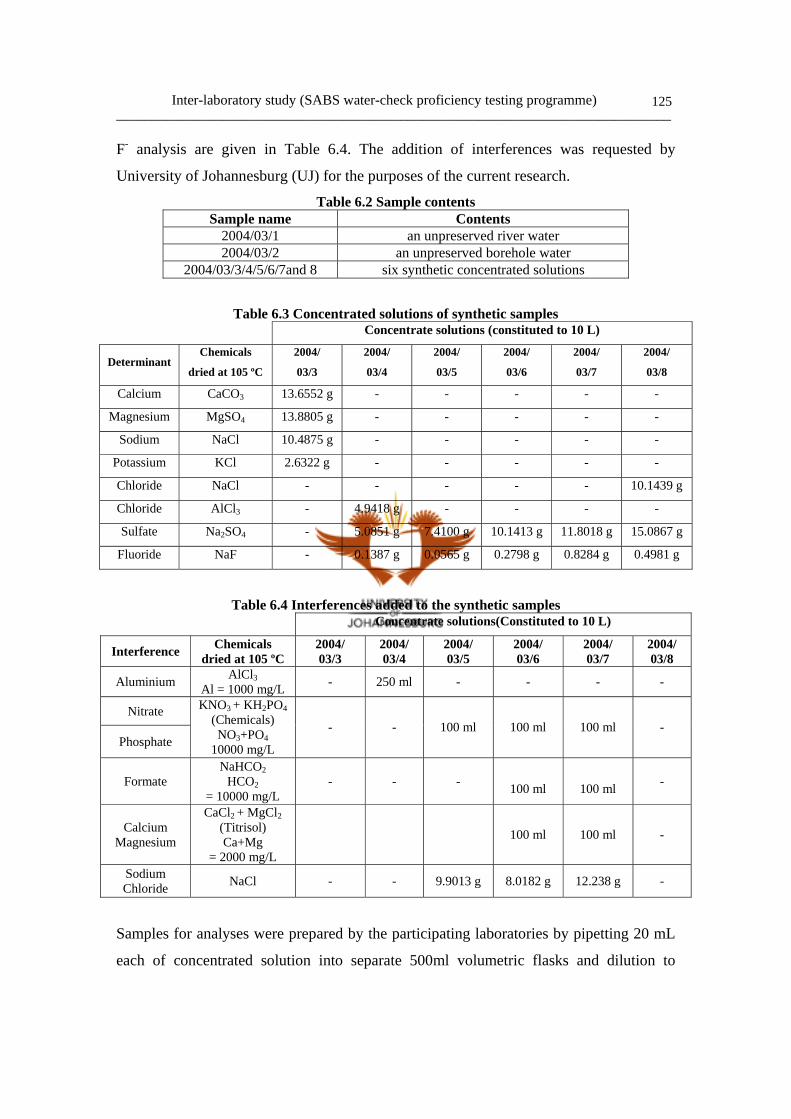
Inter-laboratory study (SABS water-check proficiency testing programme) ______________________________________________________________________________
125
F- analysis are given in Table 6.4. The addition of interferences was requested by
University of Johannesburg (UJ) for the purposes of the current research.
Table 6.2 Sample contents Sample name Contents
2004/03/1 an unpreserved river water 2004/03/2 an unpreserved borehole water
2004/03/3/4/5/6/7and 8 six synthetic concentrated solutions
Table 6.3 Concentrated solutions of synthetic samples Concentrate solutions (constituted to 10 L)
Determinant Chemicals
dried at 105 ºC
2004/
03/3
2004/
03/4
2004/
03/5
2004/
03/6
2004/
03/7
2004/
03/8
Calcium CaCO3 13.6552 g - - - - -
Magnesium MgSO4 13.8805 g - - - - -
Sodium NaCl 10.4875 g - - - - -
Potassium KCl 2.6322 g - - - - -
Chloride NaCl - - - - - 10.1439 g
Chloride AlCl3 - 4.9418 g - - - -
Sulfate Na2SO4 - 5.0851 g 7.4100 g 10.1413 g 11.8018 g 15.0867 g
Fluoride NaF - 0.1387 g 0.0565 g 0.2798 g 0.8284 g 0.4981 g
Table 6.4 Interferences added to the synthetic samples Concentrate solutions(Constituted to 10 L)
Interference Chemicals dried at 105 ºC
2004/ 03/3
2004/ 03/4
2004/ 03/5
2004/ 03/6
2004/ 03/7
2004/ 03/8
Aluminium AlCl3 Al = 1000 mg/L - 250 ml - - - -
Nitrate
Phosphate
KNO3 + KH2PO4 (Chemicals) NO3+PO4
10000 mg/L
- - 100 ml 100 ml 100 ml -
Formate NaHCO2
HCO2 = 10000 mg/L
- - - 100 ml
100 ml -
Calcium Magnesium
CaCl2 + MgCl2 (Titrisol) Ca+Mg
= 2000 mg/L
100 ml 100 ml -
Sodium Chloride NaCl - - 9.9013 g 8.0182 g 12.238 g -
Samples for analyses were prepared by the participating laboratories by pipetting 20 mL
each of concentrated solution into separate 500ml volumetric flasks and dilution to

Inter-laboratory study (SABS water-check proficiency testing programme) ______________________________________________________________________________
126
volume with distilled/ deionised water. All volumetric glassware used in the preparation
of stock standards and samples are Grade A and have been verified as complying with
their relevant standard specification. All chemicals used are AR grade chemicals supplied
by Merck, Riedel-de Haën, Fluka and BDH. Prepared stock standard solution, where used,
are supplied by Merck (Titrosol), Riedel-de-Haën, (Fixanal) or Fluka.
b. Sample dispatch
Samples were dispatched to the participation laboratories on 1 March 2004. The return
date for results was set for 31 March 2004.
6.2.2 Statistical evaluation of results
a. Introduction
The use of Robust Statistics was evaluated in the June 1997 study and found to be
effective in down weighting outlying data without excluding such data from the
evaluation. The Water-Check program now makes use of such statistics for data
evaluation. For this study, all the original values, outliers included, were recaptured
electronically in the reporting process adopted by the SABS.
b. Z-scores
The report on each study consists of a robust statistical analysis of results, with the
inclusion of outliers, against the median or true value. The Z-score for each result is
tabulated and then summarized for each laboratory. The Z-scores are calculated for all
data based on distribution of the results around the Robust Mean (Median), (x- x )/s, or
around the assigned or true value, (x-t)/s. The assigned or true value will only be used
when a synthetic sample is analyzed. The mean value will be used for all other samples,
including spiked samples.
Table 6.5 Z-score criteria Z-score Status
Z<2 Satisfactory 2<Z<3 Questionable Z> 3 Unsatisfactory
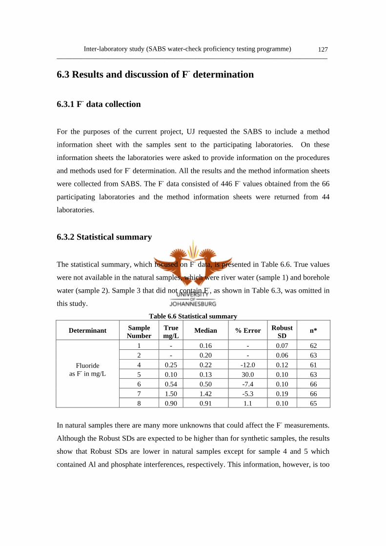
Inter-laboratory study (SABS water-check proficiency testing programme) ______________________________________________________________________________
127
6.3 Results and discussion of F- determination
6.3.1 F- data collection
For the purposes of the current project, UJ requested the SABS to include a method
information sheet with the samples sent to the participating laboratories. On these
information sheets the laboratories were asked to provide information on the procedures
and methods used for F- determination. All the results and the method information sheets
were collected from SABS. The F- data consisted of 446 F- values obtained from the 66
participating laboratories and the method information sheets were returned from 44
laboratories.
6.3.2 Statistical summary
The statistical summary, which focused on F- data, is presented in Table 6.6. True values
were not available in the natural samples, which were river water (sample 1) and borehole
water (sample 2). Sample 3 that did not contain F-, as shown in Table 6.3, was omitted in
this study.
Table 6.6 Statistical summary
Determinant Sample Number
Truemg/L
Median % Error Robust SD
n*
1 - 0.16 - 0.07 62 2 - 0.20 - 0.06 63 4 0.25 0.22 -12.0 0.12 61 5 0.10 0.13 30.0 0.10 63 6 0.54 0.50 -7.4 0.10 66 7 1.50 1.42 -5.3 0.19 66
Fluoride
as F- in mg/L
8 0.90 0.91 1.1 0.10 65
In natural samples there are many more unknowns that could affect the F- measurements.
Although the Robust SDs are expected to be higher than for synthetic samples, the results
show that Robust SDs are lower in natural samples except for sample 4 and 5 which
contained Al and phosphate interferences, respectively. This information, however, is too
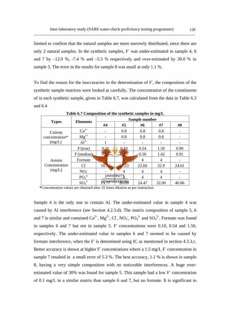
Inter-laboratory study (SABS water-check proficiency testing programme) ______________________________________________________________________________
128
limited to confirm that the natural samples are more narrowly distributed, since there are
only 2 natural samples. In the synthetic samples, F- was under-estimated in sample 4, 6
and 7 by –12.0 %, -7.4 % and –5.3 % respectively and over-estimated by 30.0 % in
sample 5. The error in the results for sample 8 was small at only 1.1 %.
To find the reason for the inaccuracies in the determination of F-, the composition of the
synthetic sample matrices were looked at carefully. The concentration of the constituents
of in each synthetic sample, given in Table 6.7, was calculated from the data in Table 6.3
and 6.4
Table 6.7 Composition of the synthetic samples in mg/L Sample number Types Elements
#4 #5 #6 #7 #8 Ca2+ - 0.8 0.8 0.8 - Mg2+ - 0.8 0.8 0.8 -
Cations concentration*
(mg/L) Al3+ 1 - - - - F-(true) 0.25 0.10 0.54 1.50 0.90
F-(median) 0.22 0.13 0.50 1.42 0.91 Formate - - 4 4 -
Cl- 18.77 27.23 22.66 32.9 24.61 NO3
- - 4 4 4 - PO4
3- - 4 4 4 -
Anions
Concentration(mg/L)
SO42- 13.77 20.09 24.47 32.00 40.86
*Concentration values are obtained after 25 times dilution as per instruction
Sample 4 is the only one to contain Al. The under-estimated value in sample 4 was
caused by Al interference (see Section 4.2.3.d). The matrix composition of sample 5, 6
and 7 is similar and contained Ca2+, Mg2+, Cl-, NO3-, PO4
3- and SO42-. Formate was found
in samples 6 and 7 but not in sample 5. F- concentrations were 0.10, 0.54 and 1.50,
respectively. The under-estimated value in samples 6 and 7 seemed to be caused by
formate interference, when the F- is determined using IC as mentioned in section 4.3.3.c.
Better accuracy is shown at higher F- concentrations where a 1.5 mg/L F- concentration in
sample 7 resulted in a small error of 5.3 %. The best accuracy, 1.1 % is shown in sample
8, having a very simple composition with no noticeable interferences. A huge over-
estimated value of 30% was found for sample 5. This sample had a low F- concentration
of 0.1 mg/L in a similar matrix than sample 6 and 7, but no formate. It is significant to

Inter-laboratory study (SABS water-check proficiency testing programme) ______________________________________________________________________________
129
notice that the F- concentration in sample 5 was the lowest value of all the synthetic
samples. Therefore a seemingly small change in the second decimal digit can cause a
significant relative error of 30% at this level. There are no obvious interferences that can
cause over-estimated F- value in sample 5, therefore the overestimated results seem to be
caused by measuring error at low-level determination of F-.
6.3.3 Comparison of analytical methods
Data from the method information sheets, returned from 44 out of 66 laboratories, were
analyzed to compare the correlation between accuracy and analytical method. The
methods used by the different laboratories are listed in Table 6.8.
Table 6.8 Analytical methods for F- determination in this study Analytical methods Number of laboratories %
ISE 18 40 IC 16 36
SPAND 8 18 Others 3 7
Total numbers* 45 100 *Lab X: Double-counted since it used both ISE and IC method, therefore total number became 45
Of all the results returned to the SABS, 40 % was obtained by the ISE method, 36 % by
the IC, 8 % by the SPANDS method, and the remaining 7% by other methods. Absolute
Z-scores and analytical method used by each laboratory are summarized in Table 6.9.
Table 6.9 Average Z-score and analytical method Order Lab code Average Z-score (Absolute value) Analytical method
1 X(ISE) 0.18 ISE 2 B104 0.22 ISE 3 B1 0.23 Undisclosed 4 B49 0.24 ISE 5 X(IC) 0.27 IC 6 B108 0.27 ISE 7 B10 0.28 ISE 8 B6 0.30 ISE 9 B22 0.31 ISE
10 B86 0.36 IC 11 B65 0.38 Undisclosed 12 B25 0.40 Undisclosed 13 B63 0.43 IC 14 B23 0.44 SPANDS
Inter-laboratory study (SABS water-check proficiency testing programme) ______________________________________________________________________________
130
15 B26 0.44 Undisclosed 16 B3 0.47 ISE 17 B5 0.48 ISE 18 B91 0.49 IC 19 B109 0.49 Undisclosed 20 B11 0.51 ISE 21 B28 0.55 SPANDS 22 B8 0.56 Undisclosed 23 B59 0.58 SPANDS 24 B68 0.59 ISE 25 B130 0.59 Undisclosed 26 B14 0.62 IC 27 B33 0.70 ISE 28 B70 0.72 Undisclosed 29 B100 0.72 Undisclosed 30 B80 0.76 Undisclosed 31 B47 0.77 DR Lange 32 B9 0.79 ISE 33 B34 0.79 IC 34 B39 0.86 Undisclosed 35 B102 0.87 Undisclosed 36 B103 0.93 Undisclosed 37 B19 0.95 Undisclosed 38 B41 0.96 SPANDS 39 B21 1.07 IC 40 B125 1.11 Undisclosed 41 B44 1.13 Probe 42 B99 1.18 SPANDS 43 B112 1.19 SPANDS 44 B101 1.20 SPANDS 45 B123 1.20 Undisclosed 46 B105 1.21 Undisclosed 47 B76 1.28 Undisclosed 48 B117 1.32 IC 49 B45 1.55 Undisclosed 50 B73 1.58 CIA 51 B42 1.62 IC 52 B94 1.65 IC 53 B92 1.70 ISE 54 B132 1.89 IC 55 B16 1.95 IC 56 B74 1.96 ISE 57 B31 2.13 IC 58 B122 2.14 ISE 59 B36 2.23 IC 60 B131 2.37 Undisclosed 61 B115 2.83 ISE 62 B71 3.15 IC 63 B29 3.48 ISE 64 B27 3.88 SPANDS 65 B78 6.66 Undisclosed 66 B116 7.72 Undisclosed 67 B119 13.08 IC

Inter-laboratory study (SABS water-check proficiency testing programme) ______________________________________________________________________________
131
The Z-score can be a useful indication for the accuracy of measurement. A smaller Z-
score indicates a better accuracy. The results using the ISE method show good accuracy
and low Z-scores. Among the top 10 lowest Z-scores, 7 laboratories used ISE and 2 used
IC method. The overall average absolute Z-score according to the analytical method is
given in Table 6.10.
Table 6.10 Average absolute Z-score with method Method Average z-score
ISE 0.98 IC 1.33
SPANDS 1.25
The IC Z-score value, 1.33, was obtained after excluding the value of lab B119, being too
high, at 13.08. The average Z-score of SPANDS is slightly lower than that of IC.
The performance of the analytical laboratories in South Africa, participating in this
proficiency testing exercise for the measurement of F-, is summarized in Table 6.11. 84%
of laboratories in this study reported satisfactory results. A graphical presentation of Z-
scores obtained by the 66 laboratories is given in Figure 6.1.
Table 6.11 Laboratory performance Z-score Status Numbers of laboratories %
Z<2 Satisfactory 56 84 2<Z<3 Questionable 5 7 Z> 3 Unsatisfactory 6 9
Total 67 100 Figure 6.1 Average absolute Z–score
Average absolute Z-score for all participants
0
1
2
3
X(ISE)B10
4 B1B49
X(IC)B10
8B10 B6
B22 B86 B65 B25 B63 B23 B26 B3 B5B91
B109B11 B28 B8
B59 B68B13
0B14 B33 B70
B100B80 B47 B9
B34 B39B10
2B10
3B19 B41 B21
B125B44 B99
B112B10
1B12
3B10
5B76
B117B45 B73 B42 B94 B92
B132B16 B74 B31
B122B36
B131B11
5B71 B29 B27 B78
B116B11
9
Lab code
Aver
age
abso
lute
Z-s
core

Inter-laboratory study (SABS water-check proficiency testing programme) ______________________________________________________________________________
132
Lab X, the first ranked, was the UJ lab and both results using ISE and IC methods from
this lab are excellent. This showed the proficiency of the procedures developed in this
study.
6.3.4 Determination of composition of natural water samples
a. Experimental method
The water-check samples, received from SABS, were analyzed further to determine
whether elements present in the samples could cause interferences. ICP-OES was used to
determine the cation elemental composition in natural samples 1 and 2. Multi-element
calibration using a Varian Liberty 100 ICP-OES spectrometer was used for the
determination of the elements: Li, B, Na, Mg, Al, Ca, Cr, Mn, Fe, Co, Ni, Cu, Zn, Sr, Ba,
Cd, Pb and Bi. A 1000 mg/L Multi IV (Merck SA) multi-element ICP-OES standard was
used to prepare calibration standards by appropriate dilution with 2% HNO3. The
experimental conditions used in ICP-OES measurements are summarized in Table 6.12.
Table 6.12 ICP-OES operational conditions Parameter Setting
Viewing height 6 mm Search window 0.04 nm
Generator power 1.20 kW Plasma gas flow rate 15.0 L/min
Auxiliary gas flow rate 1.50 L/min Pump speed 25.0 rpm
A Dionex DX-120 Ion Chromatographic system, equipped with a Dionex anion exchange
column system (AG 14A+AS14A), was used for the determination of the anions:: F-,
Formate, Cl-, Br-, NO3-, NO2
-, PO43-, SO4
2- in the natural samples. The standard HCO3
-
/CO32- (1.0 mM HCO3
- + 3.5mM CO32-) eluent recommended for anion determinations
with this column was used in all determinations.
b. Results
The results are summarized in Table 6.13 for those species in sample 1 and 2 where the
concentrations were more than the Method Detection Limit (MDL).
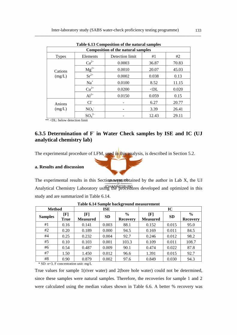
Inter-laboratory study (SABS water-check proficiency testing programme) ______________________________________________________________________________
133
Table 6.13 Composition of the natural samples Composition of the natural samples
Types Elements Detection limit #1 #2 Ca2+ 0.0003 36.87 70.83 Mg2+ 0.0010 20.07 45.03 Sr2+ 0.0002 0.038 0.13 Na+ 0.0100 8.52 11.15 Cu2+ 0.0200 <DL 0.020
Cations (mg/L)
Al3+ 0.0150 0.059 0.15 Cl- - 6.27 20.77 Anions
(mg/L) NO3- - 3.39 26.41
SO42- - 12.43 29.11
** <DL: below detection limit
6.3.5 Determination of F- in Water Check samples by ISE and IC (UJ analytical chemistry lab)
The experimental procedure of LFM, used in this analysis, is described in Section 5.2.
a. Results and discussion
The experimental results in this Section were obtained by the author in Lab X, the UJ
Analytical Chemistry Laboratory using the procedures developed and optimized in this
study and are summarized in Table 6.14.
Table 6.14 Sample background measurement Method ISE IC
Samples [F] True
[F] Measured SD %
Recovery[F]
Measured SD % Recovery
#1 0.16 0.141 0.003 88.1 0.152 0.015 95.0 #2 0.20 0.189 0.000 94.5 0.169 0.011 84.5 #4 0.25 0.232 0.004 92.7 0.246 0.012 98.2 #5 0.10 0.103 0.001 103.3 0.109 0.011 108.7 #6 0.54 0.487 0.009 90.1 0.474 0.022 87.8 #7 1.50 1.450 0.012 96.6 1.391 0.015 92.7 #8 0.90 0.879 0.002 97.6 0.849 0.030 94.3
* SD: n=3, F concentration unit: mg/L
True values for sample 1(river water) and 2(bore hole water) could not be determined,
since these samples were natural samples. Therefore, the recoveries for sample 1 and 2
were calculated using the median values shown in Table 6.6. A better % recovery was
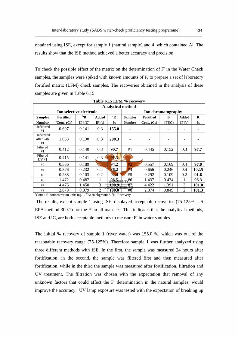
Inter-laboratory study (SABS water-check proficiency testing programme) ______________________________________________________________________________
134
obtained using ISE, except for sample 1 (natural sample) and 4, which contained Al. The
results show that the ISE method achieved a better accuracy and precision.
To check the possible effect of the matrix on the determination of F- in the Water Check
samples, the samples were spiked with known amounts of F, to prepare a set of laboratory
fortified matrix (LFM) check samples. The recoveries obtained in the analysis of these
samples are given in Table 6.15.
Table 6.15 LFM % recovery Analytical method
Ion selective electrode Ion chromatography Samples Fortified bB Added cR Samples Fortified B Added R Number aConc. (Cs) [F] (C) [F](s) % Number Conc. (Cs) [F](C) [F](s) %
Unfiltered #1 0.607 0.141 0.3 155.0 - - - - -
Unfiltered after 24h
#1 1.033 0.138 0.3 298.3 - - - - -
Filtered #1 0.412 0.140 0.3 90.7 #1 0.445 0.152 0.3 97.7
Filtered UV #1 0.415 0.141 0.3 91.3 - - - - -
#2 0.566 0.189 0.4 94.2 #2 0.557 0.169 0.4 97.0#4 0.576 0.232 0.4 86.2 #4 0.656 0.246 0.4 102.5#5 0.288 0.103 0.2 92.4 #5 0.292 0.109 0.2 91.6#6 1.472 0.487 1 98.5 #6 1.437 0.474 1 96.3#7 4.476 1.450 3 100.9 #7 4.422 1.391 3 101.0#8 2.879 0.879 2 100.0 #8 2.874 0.849 2 101.3
aConc.: F- concentration unit: mg/L, bB: Backgraound, cR: Recovery
The results, except sample 1 using ISE, displayed acceptable recoveries (75-125%, US
EPA method 300.1) for the F- in all matrices. This indicates that the analytical methods,
ISE and IC, are both acceptable methods to measure F- in water samples.
The initial % recovery of sample 1 (river water) was 155.0 %, which was out of the
reasonable recovery range (75-125%). Therefore sample 1 was further analyzed using
three different methods with ISE. In the first, the sample was measured 24 hours after
fortification, in the second, the sample was filtered first and then measured after
fortification, while in the third the sample was measured after fortification, filtration and
UV treatment. The filtration was chosen with the expectation that removal of any
unknown factors that could affect the F- determination in the natural samples, would
improve the accuracy. UV lamp exposure was tested with the expectation of breaking up

Inter-laboratory study (SABS water-check proficiency testing programme) ______________________________________________________________________________
135
the organic material in natural samples. The recoveries improved to 90.7% and 91.3%,
respectively, after filtration and filtration with UV lamp exposure. However, the result 24
hours after fortification was the least impressive, 298 %, and was in fact worse than
before. This indicated that filtration was necessary in natural river water samples for
accurate F- measurement, although not the case in the synthetic samples with ISE. Sample
2 (borehole water), another natural sample, showed a reasonable LFM recovery value,
even without filtration. It is therefore clear that the matrix could affect the analytical
results for F- determination, even though the analytical method was accurate enough.
When the ion composition of these samples was compared (Table 6.13), sample 2
contained a larger concentration of each element. Even though a lower concentration of
ions occurred in the river water sample, the LFM recovery value was out of the
acceptable recovery range. This means that there were other factors that caused the
erroneous LFM value in the river water sample. This problem could be solved by
filtration.
In the case of synthetic samples, the recovery for sample 4, which contained Al
interference, was lower 86.2%, for ISE determination, than for the other samples. This
occurred because of the formation of Al-F complexes and the less than 100% efficiency
of the decomplexing agent to break up the complex (see Section 4.2.3.d). In the case of
IC the recovery of sample 4 was 102.5 %. This is because the Al can complex with F-
strongly in the acidic medium used in ISE applied to, but no Al-F complex forms at pH 9
(IC conditions) with the less than 19 mg/L F- and 1 mg/L or 10 mg/L Al as shown in
Figure 5.9 and Figure 5.10. This means that Al is not problematic in the determination of
F-, using IC in terms of interference, but the precipitation of Al hydroxide in basic
medium should be considered, since precipitation could damage the column.
The recoveries for sample 5 were lower for both methods 92.4 % and 91.6 %, because of
a very low-level of F-, 0.10 mg/L.
Inter-laboratory study (SABS water-check proficiency testing programme) ______________________________________________________________________________
136
The other synthetic samples, 6, 7 and 8, yielded good results, close to 100 % recovery.
These samples did not display any significant interference that could result in serious
error.
6.4 Conclusion The Inter-laboratory study undertaken in collaboration with SABS (Chapter 6) was
carried out to evaluate the proficiency of South African analytical laboratories and to
check the proficiency of the procedures developed in this study as well as to establish
how different analytical methods for F- determination cope with interferences such as Al.
SABS water check F- samples data, from 66 participant laboratories, were analyzed
statistically. The most serious errors (+30%) were obtained in sample 5 containing 0.1
mg/L F-, which was very low-level and in sample 4 which contained 2.5 mg/L F- together
with 1mg/L Al interference. The F- results were obtained using various methods: 40%
from ISE, 35% from IC and 7% from SPADNS method. The ISE method is mostly used
in South African laboratories for determination of F-. The 84% of participants gave a
satisfactory result where the Z-score, the parameter for the accuracy, was less than 2. The
best average absolute Z-score was achieved when the ISE method was applied to
determine the F- in the water samples. This showed a good agreement with the conclusion
from Chapter 4 and Chapter 5, which indicated that ISE was the recommended
methodology for the accurate F- determination at low level. Lab X (UJ Analytical
chemistry lab) which applied the procedure developed in Chapter 4, showed the best
accuracy using ISE. This proved the proficiency of the procedures developed in this study.
It should be kept in mind that it is to be expected that it would be the “best” laboratories
or accredited laboratories that would be participating in proficiency testing schemes. The
relatively good results obtained in this study for the proficiency of laboratories in South
Africa to determine low level F-, could therefore reflect an over optimistic picture.
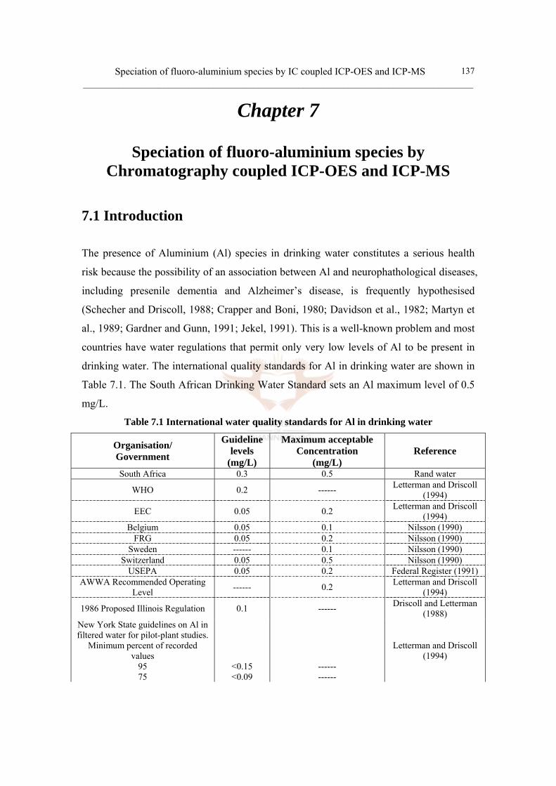
Speciation of fluoro-aluminium species by IC coupled ICP-OES and ICP-MS ______________________________________________________________________________
137
Chapter 7
Speciation of fluoro-aluminium species by Chromatography coupled ICP-OES and ICP-MS
7.1 Introduction The presence of Aluminium (Al) species in drinking water constitutes a serious health
risk because the possibility of an association between Al and neurophathological diseases,
including presenile dementia and Alzheimer’s disease, is frequently hypothesised
(Schecher and Driscoll, 1988; Crapper and Boni, 1980; Davidson et al., 1982; Martyn et
al., 1989; Gardner and Gunn, 1991; Jekel, 1991). This is a well-known problem and most
countries have water regulations that permit only very low levels of Al to be present in
drinking water. The international quality standards for Al in drinking water are shown in
Table 7.1. The South African Drinking Water Standard sets an Al maximum level of 0.5
mg/L.
Table 7.1 International water quality standards for Al in drinking water
Organisation/ Government
Guideline levels
(mg/L)
Maximum acceptable Concentration
(mg/L) Reference
South Africa 0.3 0.5 Rand water
WHO 0.2 ------ Letterman and Driscoll (1994)
EEC 0.05 0.2 Letterman and Driscoll (1994)
Belgium 0.05 0.1 Nilsson (1990) FRG 0.05 0.2 Nilsson (1990)
Sweden ------ 0.1 Nilsson (1990) Switzerland 0.05 0.5 Nilsson (1990)
USEPA 0.05 0.2 Federal Register (1991)AWWA Recommended Operating
Level ------ 0.2 Letterman and Driscoll (1994)
1986 Proposed Illinois Regulation 0.1 ------ Driscoll and Letterman (1988)
New York State guidelines on Al in filtered water for pilot-plant studies.
Minimum percent of recorded values
95 75
<0.15 <0.09
------ ------
Letterman and Driscoll (1994)
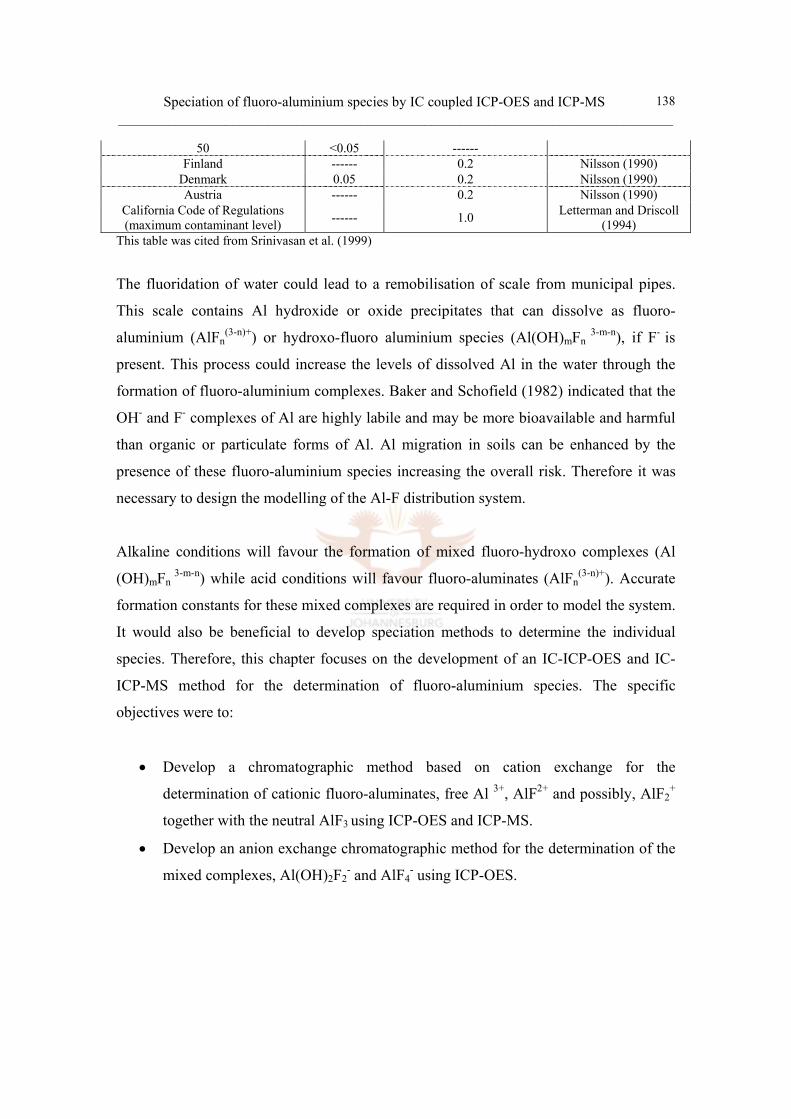
Speciation of fluoro-aluminium species by IC coupled ICP-OES and ICP-MS ______________________________________________________________________________
138
50 <0.05 ------ Finland ------ 0.2 Nilsson (1990)
Denmark 0.05 0.2 Nilsson (1990) Austria ------ 0.2 Nilsson (1990)
California Code of Regulations (maximum contaminant level) ------ 1.0 Letterman and Driscoll
(1994) This table was cited from Srinivasan et al. (1999)
The fluoridation of water could lead to a remobilisation of scale from municipal pipes.
This scale contains Al hydroxide or oxide precipitates that can dissolve as fluoro-
aluminium (AlFn(3-n)+) or hydroxo-fluoro aluminium species (Al(OH)mFn
3-m-n), if F- is
present. This process could increase the levels of dissolved Al in the water through the
formation of fluoro-aluminium complexes. Baker and Schofield (1982) indicated that the
OH- and F- complexes of Al are highly labile and may be more bioavailable and harmful
than organic or particulate forms of Al. Al migration in soils can be enhanced by the
presence of these fluoro-aluminium species increasing the overall risk. Therefore it was
necessary to design the modelling of the Al-F distribution system.
Alkaline conditions will favour the formation of mixed fluoro-hydroxo complexes (Al
(OH)mFn 3-m-n) while acid conditions will favour fluoro-aluminates (AlFn
(3-n)+). Accurate
formation constants for these mixed complexes are required in order to model the system.
It would also be beneficial to develop speciation methods to determine the individual
species. Therefore, this chapter focuses on the development of an IC-ICP-OES and IC-
ICP-MS method for the determination of fluoro-aluminium species. The specific
objectives were to:
• Develop a chromatographic method based on cation exchange for the
determination of cationic fluoro-aluminates, free Al 3+, AlF2+ and possibly, AlF2+
together with the neutral AlF3 using ICP-OES and ICP-MS.
• Develop an anion exchange chromatographic method for the determination of the
mixed complexes, Al(OH)2F2- and AlF4
- using ICP-OES.

Speciation of fluoro-aluminium species by IC coupled ICP-OES and ICP-MS ______________________________________________________________________________
139
7.2 Literature review
Dissolved Al species are complex, and can include complexes with natural organic matter,
F-, PO43-, SO4
2-, and OH-. Many authors recognized that the presence of F- could
markedly enhance Al transport in natural surface waters and in crustal fluids (Mitrovic
and Milacic, 2000; Moine et al., 1998; Zaraisky, 1994; Tennakone et al., 1988). The
presence of F- in aqueous solutions results in an increase in dissolution rates of
aluminium oxides and oxyhydroxides (Kraener et al., 1998; Nordin et al., 1998).
Roberson and Hem (1969) reported that for acidic pH (pH 5.8) and high F- concentration
(F ≥ 0.23 mg/L), complexation reactions between Al and F- are very efficient. Al-F
complexes are soluble and could potentially increase residual Al concentrations. Due to
the toxicity of Al and the existence of various fluoro-aluminium complexes, it is
generally agreed that knowledge of the form of Al species in the water system is of vital
importance.
Fluoride Ion Selective Electrode (F-ISE) has been applied to the estimation of fluoro-
aluminium complexes (Driscoll, 1984; Lazerte, 1984; Hodges, 1987; Ritchie et al., 1988).
Moore and Ritchie (1988) estimated fluoro-aluminium complexes by measuring F- with a
F-ISE before and after adding TISAB. Different methods for determining monomeric
fluoro-aluminium species have been tried, but they were indirect and usually required
speciation calculations (Hodges, 1987).
One way of achieving direct separation is to use ion chromatography (IC).The main
concern using this approach is the kinetic stability of the various fluoro-aluminium
species during the chromatography. The advantage of using IC is the direct determination
of the complexes in stead of relying solely on thermodynamic calculations.
A number of papers have been published concerning IC separation and detection by
UV/VIS spectrophotometry of fluoro-aluminium species using a variety of post-column
reactions to generate chromophores (Bertsch and Anderson, 1989; Willett, 1989; Jones,
1991; Motellier and Pitsch, 1994; Borrmann and Seubert, 1996). A post-column reaction
Speciation of fluoro-aluminium species by IC coupled ICP-OES and ICP-MS ______________________________________________________________________________
140
technique for Al involves the in-line addition of an indicator reagent, such as Tiron (4,5-
dihydroxy-m-benzene disulfonic acid) and Pyrocatechol Violet, to the separator column
effluent (Kawase et al., 1981; Application Note 42, 1986; Bertsch and Anderson, 1988;
Dean, 1989; Tapparo and Bombi, 1990). Both of these reagents are very selective for Al,
and they are useful for minimizing matrix interferences and determining Al in the
presence of other metals.
The chromatographic separation of fluoro-aluminium species was first proposed by
Bertsch and Anderson (1989), who determined the stability constants of several possible
AlFx species. They evaluated an IC method for fluoro-, oxalato-, and citrato- complexes
of Al. This method in which Al was quantitatively determined via post-column
derivatization with Tiron (4,5-dihydrozy-m-benzenedisulfonic acid) was evaluated for its
utility as a method for speciating Al in aqueous solution. However, adjustments to bring
sample ionic strength and pH to that of the eluent were required to prevent redistribution
of the species during determination. This separation was achieved by using a Dionex CS-
3 (4.6×200mm) separator column with 0.7 M NH4Cl eluent, adjusted to pH 2.0, 3.2, or
4.2 with HCl, at a flow rate of 1.0 mL/min. A CG 3 (4.6×50 mm) was also utilized with
weaker eluents (0.4 M NH4Cl). Improved chromatographic resolution of the AlF2+ and
AlF2+ species was achieved when a lower ionic strength (µ) eluent (0.4 M) was used,
though the use of the lower µ eluent tended to broaden the Al3+ peak. The comparison
with thermodynamic calculations gave results consistent with the formation of AlF2+ and
AlF2+ species.
In a similar way Willet (1989) also employed an IC method, using CG-2 column based
on a sulfate eluent, followed by the post-column reaction with pyrocatechol violet, but
without the adjustment of sample ionic strength and pH to match the eluent. The
chromatograms showed the effects of increasing F- concentrations on 40 µM Al, and the
appearance of peaks for fluoro-aluminium species at the expense of Al3+. However, the
resolution of first two peaks, AlF2+ and AlF2+ species, was not good enough for accurate
integration.
Speciation of fluoro-aluminium species by IC coupled ICP-OES and ICP-MS ______________________________________________________________________________
141
Jones (1991) investigated a highly sensitive and selective short-column ion
chromatography method for the direct determination of Al species in water samples. The
eluent used was 0.09 M K2SO4, adjusted to pH 3.0 with dilute nitric acid. The pH was
adjusted to ensure that all Al ions were present as the simple Al 3+ hydrated ion that can
yield only a single peak on the chromatogram of Al standards in absence of F-. It was
concluded that if hydroxy species such as Al(OH)2+ and Al(OH)2+ were present, they
were rapidly converted to the simple hydrated Al3+ ion in the pH 3 eluent stream, thus
giving only one peak. Otherwise, fluoro-aluminium speciation can be very complicated
due to the multi peaks from Al(OH)2+ and Al(OH)2+ species. The chromatogram in this
paper revealed that the first two peaks, AlF2+ and AlF2+ species, were not quite resolved
so the author recommended that for more precise determinations of the fluoro-aluminium
species, longer columns may be required to improve resolution.
A speciation method described by Motellier and Pitsch (1994) was performed with a CS-
2 cation-exchange column protected by a CG-2 guard column. The mobile phase
consisted of 0.5 M NH4Cl - 0.01 M HCl at a flow rate 1.1 mL/min. The post-column
reagent, 3× 10⁻⁴ M Tiron in 3 M ammonium acetate, was introduced into the eluent
stream via a T-piece located at the outlet of the column, at a rate of 0.75 mL/min. This
method requires adjustment of the sample pH and ionic strength to match the mobile
phase. The acidic media was chosen to prevent aluminium-hydroxide precipitation for
cation speciation. Total Al could be determined by the sum of the areas of the three peaks
representing the Al species because the Al species are conserved whatever the amount of
F- in the sample. This suggests that sufficiently rapid kinetics of AlFn3-n dissociation and
Al-Tiron complex formation occur as these species successively react with Tiron before
reaching the detector cell. If the sample pH is low (<4.5), ionic strength and total F-
concentration have no significant influence on the accuracy of the experimental results.
With initial sample pH values higher than 5, acidification of the sample before injection
favours rapid dehydroxylation followed by fluorination of Al3+. Although the total Al
concentration is correctly deduced, the method was not suitable for speciation since the
first two peaks, AlF2+ and AlF2+, were not fully resolved.

Speciation of fluoro-aluminium species by IC coupled ICP-OES and ICP-MS ______________________________________________________________________________
142
Isocratic elution, which used a single eluent, has been employed in the papers mentioned
above. Since the first two peaks have not been separated completely by an isocratic
elution system, some authors tried to carry out the speciation using gradient elution
system. This system uses different eluents in a stepwise elution to improve peak shape
and the separation of peaks.
Borrmann and Seubert (1996) applied IC with a gradient elution system using the eluent,
perchloric acid and ethlenediamine perchlorate, for speciating Al and its fluoro, oxalate
and citrate complexes. The detection method was a post-column reaction with Tiron
followed by UV detector. The chromatogram shows a good separation of three species.
Another application of gradient elution is found in the paper written by Hara et al. (2001).
The gradient elution procedure, using the eluent HNO3 and Ca(NO3)2, produces three
distinctive peaks for an aluminium F- solution. Equilibrium distribution of fluoro-
aluminium species with variation in the concentration ratio of F- to Al is conducted
experimentally and confirmed to agree with the theoretical calculation of species
distribution.
7.3 Modelling of the Al-F-H system and calculation of
distribution curves for cationic fluoro-aluminates
7.3.1 Theoretical distribution curve
The theoretical distribution curve for the species in the Al-F-H system was calculated
using the computer programme Species-Calc (Prof Hans Rohwer, Mandela Metropolitan
University of Port Elizabeth). The species that were taken into account for this
calculation in acidic media were Al3+; AlF2+; AlF2+; AlF3; AlF4
-. The equilibria and
equilibrium constants expressions of the fluoro-aluminium species used in this
calculation are given in Table 7.2.
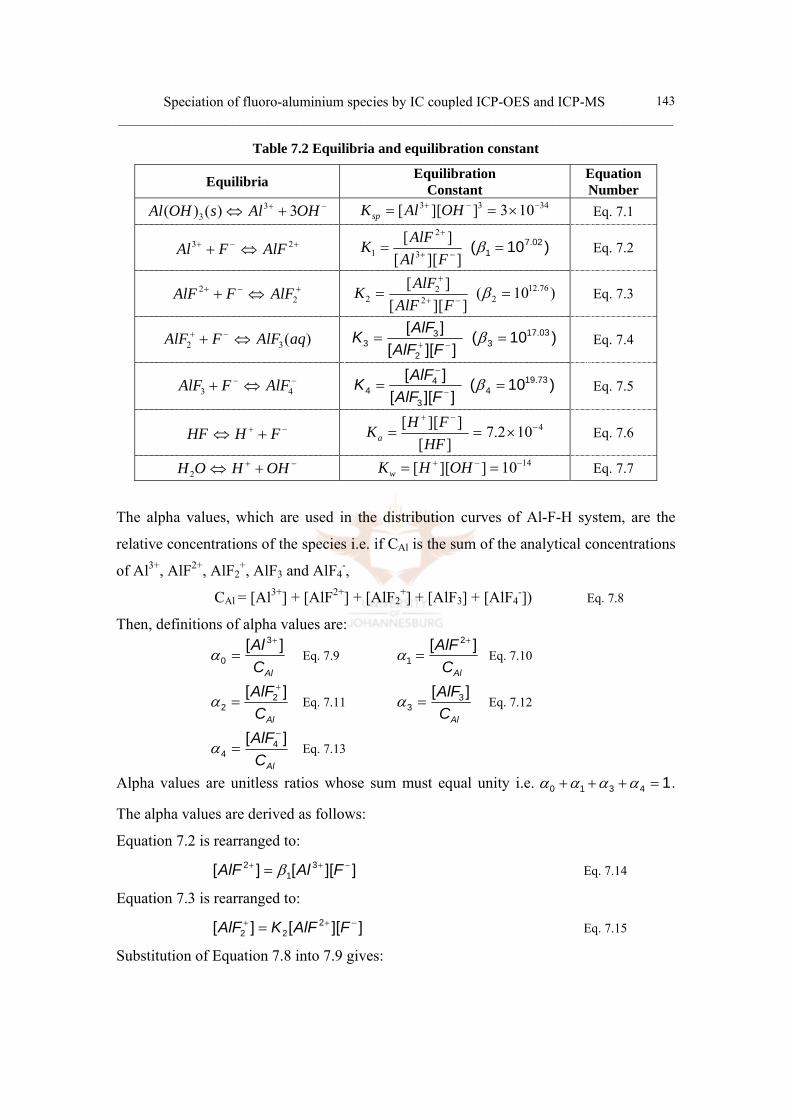
Speciation of fluoro-aluminium species by IC coupled ICP-OES and ICP-MS ______________________________________________________________________________
143
Table 7.2 Equilibria and equilibration constant
Equilibria Equilibration Constant
Equation Number
−+ +⇔ OHAlsOHAl 3)()( 33
3433 103]][[ −−+ ×== OHAlKsp Eq. 7.1
+−+ ⇔+ 23 AlFFAl ]][[
][3
2
1 −+
+
=FAl
AlFK )10( 02.71 =β Eq. 7.2
+−+ ⇔+ 22 AlFFAlF
]][[][
22
2 −+
+
=FAlF
AlFK )10( 76.122 =β Eq. 7.3
)(32 aqAlFFAlF ⇔+ −+ ]][[
][
2
33 −+=
FAlFAlFK )10( 03.17
3 =β Eq. 7.4
−− ⇔+ 43 AlFFAlF ]][[
][
3
44 −
−
=FAlF
AlFK )10( 73.194 =β Eq. 7.5
−+ +⇔ FHHF 4102.7][
]][[ −−+
×==HF
FHKa Eq. 7.6
−+ +⇔ OHHOH2 1410]][[ −−+ == OHHKw Eq. 7.7
The alpha values, which are used in the distribution curves of Al-F-H system, are the
relative concentrations of the species i.e. if CAl is the sum of the analytical concentrations
of Al3+, AlF2+, AlF2+, AlF3 and AlF4
-,
CAl = [Al3+] + [AlF2+] + [AlF2+] + [AlF3] + [AlF4
-]) Eq. 7.8
Then, definitions of alpha values are:
AlC
Al ][ 3
0
+
=α Eq. 7.9 AlC
AlF ][ 2
1
+
=α Eq. 7.10
AlC
AlF ][ 22
+
=α Eq. 7.11 AlC
AlF ][ 33 =α Eq. 7.12
AlC
AlF ][ 44
−
=α Eq. 7.13
Alpha values are unitless ratios whose sum must equal unity i.e. 14310 =+++ αααα .
The alpha values are derived as follows:
Equation 7.2 is rearranged to:
]][[][ 31
2 −++ = FAlAlF β Eq. 7.14
Equation 7.3 is rearranged to:
]][[][ 222
−++ = FAlFKAlF Eq. 7.15
Substitution of Equation 7.8 into 7.9 gives:
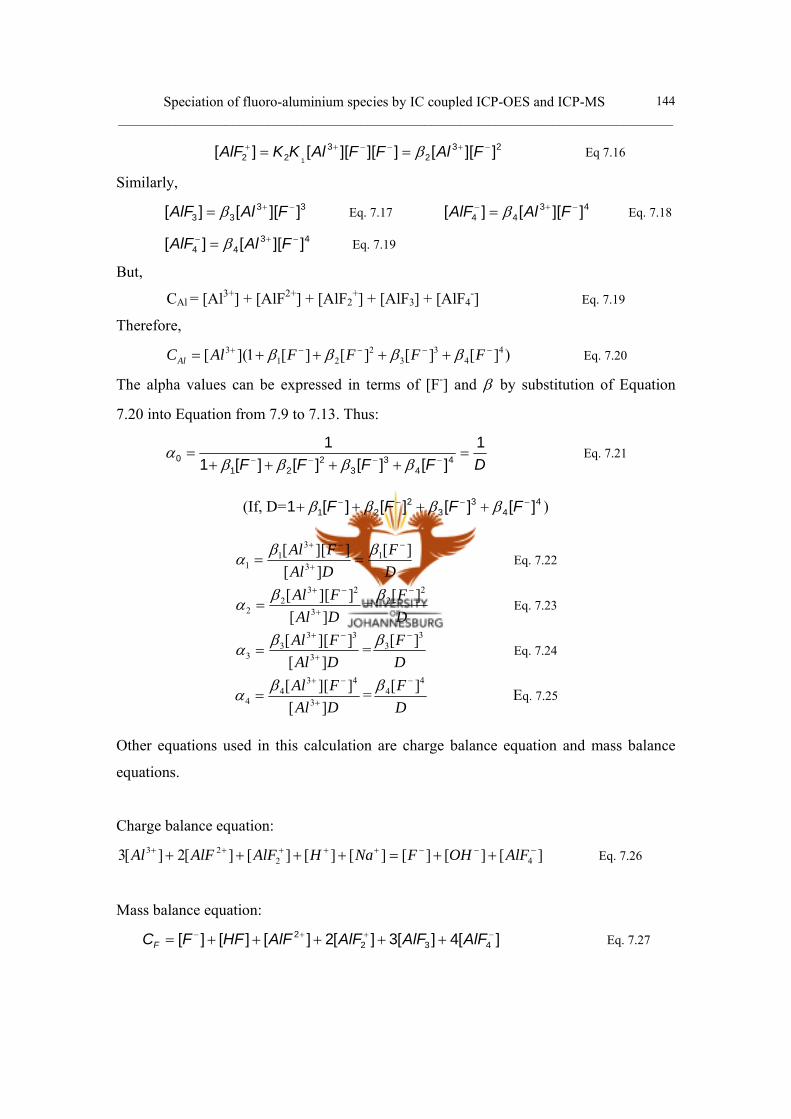
Speciation of fluoro-aluminium species by IC coupled ICP-OES and ICP-MS ______________________________________________________________________________
144
232
322 ]][[]][][[][
1
−+−−++ == FAlFFAlKKAlF β Eq 7.16
Similarly,
3333 ]][[][ −+= FAlAlF β Eq. 7.17 43
44 ]][[][ −+− = FAlAlF β Eq. 7.18
4344 ]][[][ −+− = FAlAlF β Eq. 7.19
But,
CAl = [Al3+] + [AlF2+] + [AlF2+] + [AlF3] + [AlF4
-] Eq. 7.19
Therefore,
)][][][][1]([ 44
33
221
3 −−−−+ ++++= FFFFAlCAl ββββ Eq. 7.20
The alpha values can be expressed in terms of [F-] and β by substitution of Equation
7.20 into Equation from 7.9 to 7.13. Thus:
DFFFF1
][][][][11
44
33
221
0 =++++
= −−−− ββββα Eq. 7.21
(If, D= 4
43
32
21 ][][][][1 −−−− ++++ FFFF ββββ )
DF
DAlFAl ][
][]][[ 1
3
31
1
−
+
−+
==ββα Eq. 7.22
DAlFAl
][]][[
3
232
2 +
−+
=βα =
DF 2
2 ][ −β Eq. 7.23
DAlFAl
][]][[
3
333
3 +
−+
=βα =
DF 3
3 ][ −β Eq. 7.24
DAlFAl
][]][[
3
434
4 +
−+
=βα =
DF 4
4 ][ −β Eq. 7.25
Other equations used in this calculation are charge balance equation and mass balance
equations.
Charge balance equation:
][][][][][][][2][3 4223 −−−+++++ ++=++++ AlFOHFNaHAlFAlFAl Eq. 7.26
Mass balance equation:
][4][3][2][][][ 4322 −++− +++++= AlFAlFAlFAlFHFFCF Eq. 7.27
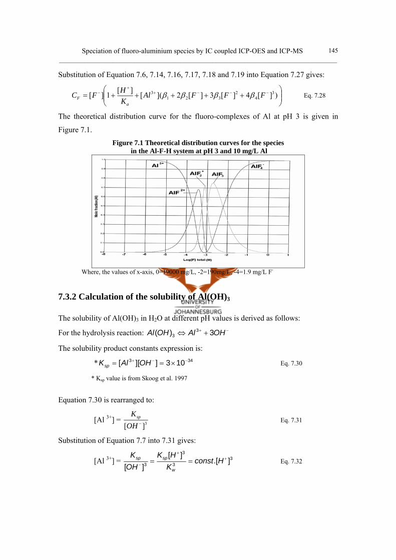
Speciation of fluoro-aluminium species by IC coupled ICP-OES and ICP-MS ______________________________________________________________________________
145
Substitution of Equation 7.6, 7.14, 7.16, 7.17, 7.18 and 7.19 into Equation 7.27 gives:
⎟⎟⎠
⎞⎜⎜⎝
⎛+++++= −−−+
+− )][4][3][2]([][1][ 3
42
3213 FFFAl
KHFC
aF ββββ Eq. 7.28
The theoretical distribution curve for the fluoro-complexes of Al at pH 3 is given in
Figure 7.1.
Figure 7.1 Theoretical distribution curves for the species in the Al-F-H system at pH 3 and 10 mg/L Al
Where, the values of x-axis, 0=19000 mg/L, -2=190mg/L, -4=1.9 mg/L F-
7.3.2 Calculation of the solubility of Al(OH)3
The solubility of Al(OH)3 in H2O at different pH values is derived as follows:
For the hydrolysis reaction: −+ +⇔ OHAlOHAl 3)( 33
The solubility product constants expression is:
* 343 103]][[ −−+ ×== OHAlKsp Eq. 7.30
* Ksp value is from Skoog et al. 1997
Equation 7.30 is rearranged to:
[Al 3+] = 3][ −OHKsp Eq. 7.31
Substitution of Equation 7.7 into 7.31 gives:
[Al 3+] = 33
3
3 ].[][
][+
+
− == HconstKHK
OHK
w
spsp Eq. 7.32
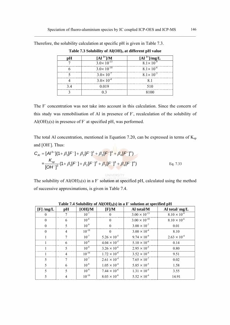
Speciation of fluoro-aluminium species by IC coupled ICP-OES and ICP-MS ______________________________________________________________________________
146
Therefore, the solubility calculation at specific pH is given in Table 7.3.
Table 7.3 Solubility of Al(OH)3 at different pH value
pH [Al 3+]/M [Al 3+]/mg/L 7 3.0×10⁻¹³ 8.1×10⁻⁹ 6 3.0×10⁻¹⁰ 8.1×10⁻⁶ 5 3.0×10⁻⁷ 8.1×10⁻³ 4 3.0×10⁻⁴ 8.1
3.4 0.019 510 3 0.3 8100
The F- concentration was not take into account in this calculation. Since the concern of
this study was remobilisation of Al in presence of F-, recalculation of the solubility of
Al(OH)3(s) in presence of F- at specified pH, was performed.
The total Al concentration, mentioned in Equation 7.20, can be expressed in terms of Ksp
and [OH-]. Thus:
)][][][][1]([ 44
33
221
3 −−−−+ ++++= FFFFAlCAl ββββ
= )][][][][1(][
44
33
2213
−−−−− ++++ FFFF
OHKsp ββββ Eq. 7.33
The solubility of Al(OH)3(s) in a F- solution at specified pH, calculated using the method
of successive approximations, is given in Table 7.4.
Table 7.4 Solubility of Al(OH)3(s) in a F- solution at specified pH [F] /mg/L pH [OH]/M [F]/M Al total/M Al total/ mg/L
0 7 10-7 0 3.00 ×10⁻¹³ 8.10 ×10⁻⁹ 0 6 10-8 0 3.00 ×10⁻¹⁰ 8.10 ×10⁻⁶ 0 5 10-9 0 3.00 ×10⁻⁷ 0.01 0 4 10-10 0 3.00 ×10⁻⁴ 8.10 1 7 10-7 5.26 ×10⁻⁵ 9.74 ×10⁻⁹ 2.63 ×10⁻⁴ 1 6 10-8 4.04 ×10⁻⁵ 5.10 ×10⁻⁶ 0.14 1 5 10-9 3.26 ×10⁻⁶ 2.95 ×10⁻⁵ 0.80 1 4 10-10 1.72 ×10⁻⁸ 3.52 ×10⁻⁴ 9.51 5 7 10-7 2.61 ×10⁻⁴ 7.65 ×10⁻⁷ 0.02 5 6 10-8 1.05 ×10⁻⁴ 5.85 ×10⁻⁵ 1.58 5 5 10-9 7.44 ×10⁻⁶ 1.31 ×10⁻⁴ 3.55 5 4 10-10 8.03 ×10⁻⁸ 5.52 ×10⁻⁴ 14.91
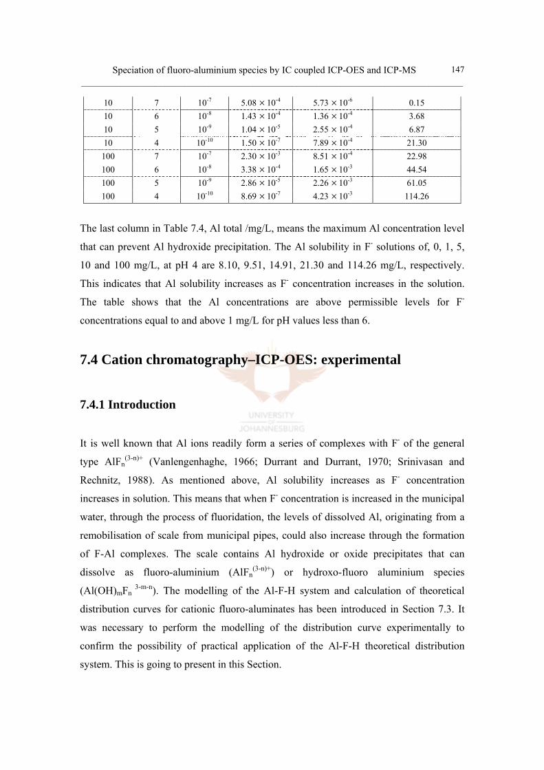
Speciation of fluoro-aluminium species by IC coupled ICP-OES and ICP-MS ______________________________________________________________________________
147
10 7 10-7 5.08 ×10⁻⁴ 5.73 ×10⁻⁶ 0.15 10 6 10-8 1.43 ×10⁻⁴ 1.36 ×10⁻⁴ 3.68 10 5 10-9 1.04 ×10⁻⁵ 2.55 ×10⁻⁴ 6.87 10 4 10-10 1.50 ×10⁻⁷ 7.89 ×10⁻⁴ 21.30 100 7 10-7 2.30 ×10⁻³ 8.51 ×10⁻⁴ 22.98 100 6 10-8 3.38 ×10⁻⁴ 1.65 ×10⁻³ 44.54 100 5 10-9 2.86 ×10⁻⁵ 2.26 ×10⁻³ 61.05 100 4 10-10 8.69 ×10⁻⁷ 4.23 ×10⁻³ 114.26
The last column in Table 7.4, Al total /mg/L, means the maximum Al concentration level
that can prevent Al hydroxide precipitation. The Al solubility in F- solutions of, 0, 1, 5,
10 and 100 mg/L, at pH 4 are 8.10, 9.51, 14.91, 21.30 and 114.26 mg/L, respectively.
This indicates that Al solubility increases as F- concentration increases in the solution.
The table shows that the Al concentrations are above permissible levels for F-
concentrations equal to and above 1 mg/L for pH values less than 6.
7.4 Cation chromatography–ICP-OES: experimental
7.4.1 Introduction
It is well known that Al ions readily form a series of complexes with F- of the general
type AlFn(3-n)+ (Vanlengenhaghe, 1966; Durrant and Durrant, 1970; Srinivasan and
Rechnitz, 1988). As mentioned above, Al solubility increases as F- concentration
increases in solution. This means that when F- concentration is increased in the municipal
water, through the process of fluoridation, the levels of dissolved Al, originating from a
remobilisation of scale from municipal pipes, could also increase through the formation
of F-Al complexes. The scale contains Al hydroxide or oxide precipitates that can
dissolve as fluoro-aluminium (AlFn(3-n)+) or hydroxo-fluoro aluminium species
(Al(OH)mFn 3-m-n). The modelling of the Al-F-H system and calculation of theoretical
distribution curves for cationic fluoro-aluminates has been introduced in Section 7.3. It
was necessary to perform the modelling of the distribution curve experimentally to
confirm the possibility of practical application of the Al-F-H theoretical distribution
system. This is going to present in this Section.
Speciation of fluoro-aluminium species by IC coupled ICP-OES and ICP-MS ______________________________________________________________________________
148
Since Bersch and Anderson (1989) proposed the separation of fluoro-aluminium species,
many authors reported this speciation mainly using the IC method (Willet, 1989; Jones,
1991; Motelier and Pitsch, 1994). However, their methods were not suitable for
speciation since the first two peaks, AlF2+ and AlF2+, were not completely resolved. The
purpose of the current work was to develop a method for the simultaneous determination
of fluoro-aluminium species, free Al 3+, AlF2+ and possibly, AlF2+ together with the
neutral AlF3. The separation was carried out on a cation exchange column and the fluoro-
aluminium species were detected by inductively coupled plasma-optical emission
spectrometry (IC-ICP-OES). The distribution curves for the fluoro-aluminium complexes,
determined experimentally by the IC-ICP-OES method, were compared with theoretical
curves based on the calculations with formation constants.
7.4.2 Instrumentation
A Dionex Gradient Pump equipped with a Rheodyne Model 9126 Injection Valve (100
µ L sample loop) was coupled to a Dionex Ion Pac CG5A and CG 5 (Serial number
5914) cation exchange column. The chromatographic columns were connected to a
Varian Liberty 110 ICP Emission Spectrometer. The flow rate was 2 mL/min. Data
capturing and peak analyses were performed with the use of Star Chromatography
Software (1995, Varian Associates Inc.).
7.4.3 Reagents and standard solutions
All reagents were of AR grade and high quality deionised water (18 MΩ) was used for
preparing all solutions. Samples and eluents were filtered through 0.22 µm membrane
filters.
The following solutions were prepared:
• 1000 mg/L Al stock solution: 0.894 g AlCl3·6H2O was dissolved in deionised
water and diluted to 100 mL in a volumetric flask

Speciation of fluoro-aluminium species by IC coupled ICP-OES and ICP-MS ______________________________________________________________________________
149
• 1000 mg/L F- Stock solution: 0.221 g NaF was dissolved in deionised water and
diluted to 100 mL in a polystyrene volumetric flask.
• Eluent (0.5 M NH4Cl, 1mM HCl): 26.745 g NH4Cl was dissolved in deionised
water and diluted to 1L with a 1 mM HCl matrix (100µ L of 32% HCl (10 M)) in
a volumetric flask.
A series of synthetic sample mixtures, 10 mg/L Al and various concentrations of F-,
were prepared by the appropriate dilution of the stock solutions with 1 mM HCl.
7.4.4 Results and discussion
a. Optimisation of ICP-OES conditions
A summary of the optimised parameters for ICP-OES is given in Table 7.5.
Table 7.5 ICP-OES operating condition Parameter Setting
Al Emission Wavelength 396.152 nm Plasma power 1.00 kW
Search window 0.040 nm Viewing height 6 mm
Plasma gas flow rate 15.0 L/min Nebuliser pressure 150 kPa
Pump speed 250 rpm Auxiliary gas flow rate 1.50 L/min
b. Optimisation of the chromatographic conditions
i) Al concentration and pH optimisation
A 1 mg/L and 10 mg/L Al solution in 0.01 M HCl was tested with the eluent 0.5M NH4Cl
and 0.01 M HCl (Motellier and Pitsch 1994) using two Dionex CS5 (Serial number 5754,
6223) analytical columns. No peak was observed at the 1 mg/L Al concentration level
with CS5 (S/N6223) and only a very small peak with CS5 (S/N 5754). This meant that
the IC coupled ICP-OES method was not sensitive enough to analyse at 1 mg/L Al level.
One big Al3+ peak, however, was obtained with the 10mg/L Al solution. In further work
and the experimental verification of the distribution diagram given in Figure 7.1, 10 mg/L
Al solution was used.

Speciation of fluoro-aluminium species by IC coupled ICP-OES and ICP-MS ______________________________________________________________________________
150
As briefly summarized in the literature review, Jones (1991) has demonstrated the
importance of pH on the fluoro-aluminium speciation (see Section 7.2). Another aspect
concerning pH, which the current work has pointed out, is the Al hydroxide precipitation
at higher pH. This precipitation can damage the column. The solubility of Al(OH)3 in
H2O and in F- solution at different pH values is described in Section 7.3.2. The last
column in Table 7.4, Al total /mg/L, presents the solubility of Al(OH)3 in various
concentrations of F- at specific pH values. The purpose of this experiment was to measure
the distribution curve over the whole range of F- at a fixed concentration of Al, 10mg/L.
It was necessary to choose a suitable pH value, which would prevent Al(OH)3
precipitation. The solubility of Al(OH)3, given in Table 7.4, in presence of 0 mg/L and 1
mg/L F- at pH 4 was 8.10 mg/L and 9.51,mg/L respectively. These values were less than
the chosen Al concentration, 10 mg/L, in previous paragraph. Therefore, the fluoro-
aluminium speciation at pH 4 or higher than pH 4 could not be performed owing to the
Al(OH)3 solubility, which was lower than the chosen Al concentration, 10 mg/L.
According to the solubility data in Table 7.3, the solubility of Al(OH)3 in 0 mg/L F- at pH
3 was 8100 mg/L. This value was high enough to prevent precipitation of Al(OH)3.
Therefore, pH 3 was chosen for further work. Wang et al. (1996) has demonstrated that in
highly acidic medium, F- reacts with H+ to form HF, leading to a decrease in the rate of
complexation of Al3+ with F-. At pH>3.0, the hydrolysis reaction of Al3+ can take place
with the formation of Al(OH)i(3-i)+, which reduces free Al and therefore the concentration
of complex.
ii) Eluent and column optimisation
Dionex CG12A and CG5A guard columns, which are shorter in length than the full
analytical column and would allow the analysis time to remain short resulting in a quick
and cost effective analysis, were chosen for fluoro-aluminium speciation studies of the
cationic species.
As previously mentioned in Section 7.2, the published methods were not suitable for
speciation since the first two peaks, AlF2+ and AlF2+, were not fully resolved to allow
accurate integration (Willet, 1989; Jones, 1991; Motellier and Pitsch, 1994). Therefore, it
Speciation of fluoro-aluminium species by IC coupled ICP-OES and ICP-MS ______________________________________________________________________________
151
was important to separate the first two peaks, i.e. for AlF2+ and AlF2+ species. The
theoretical distribution curve in Figure 7.1 shows the intersection point of these species,
AlF2+ and AlF2+, at about 10 mg/L Al and 10 mg/L F-. The intersection was a suitable
point to optimize eluent and column, since two peaks with similar sensitivity were
expected. The peak of Al3+ was not expected to show on the chromatogram, since the
alpha value of Al3+ at this point was very small, about 0.02. Therefore, the concentrations
of this point, 10 mg/L Al and 10 mg/L F-, were chosen for optimization of eluent and
column.
0.5 M NH4Cl and 0.001 M HCl, at pH 3, and a flow rate 1.2 mL/min were chosen for
speciation of Al-F species. No peak was found with the CG 12A column and overlapping
peaks with poor resolution were displayed with the CG 5A column. Therefore, these
guard columns were not suitable for separation of Al-F species. Thus, the CG 5A guard
column, which showed overlapping peaks, was used in conjunction with the CS5
analytical column. Various CS5 analytical columns, (serial number 6223, 5914 and 5754
from Dionex), were evaluated to determine the column, that provided the best
chromatographic separation, for further work. The two peaks, AlF2+ and AlF2+, were
separated with good resolution with a CG5A guard column in conjunction with a CS5
analytical column. The CS5 with serial number 5914 in conjunction with a CG5A was
found to give the best chromatographic separation.
To confirm the efficiency of these column systems in the F- concentration range, that
could display three peaks on the chromatogram, a test solution containing 10mg/L Al and
6mg/L F- was analyzed as well. The three peaks, AlF2+, AlF2+ and Al3+, were separated
with good resolution using this column system. Therefore, CG5A guard column in
conjunction with CS 5 (S/N 5914) analytical column was chosen for further work.
iii) Flow rate optimisation
A sample containing 10 mg/L Al and 10 mg/L F-, for which 2 similar size
chromatographic peaks were displayed, was used for optimisation of flow rate. Flow rates
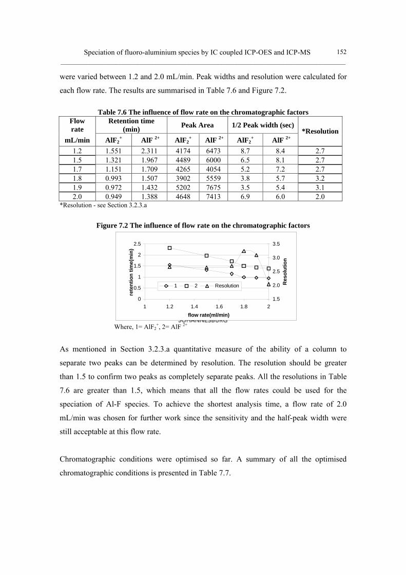
Speciation of fluoro-aluminium species by IC coupled ICP-OES and ICP-MS ______________________________________________________________________________
152
were varied between 1.2 and 2.0 mL/min. Peak widths and resolution were calculated for
each flow rate. The results are summarised in Table 7.6 and Figure 7.2.
Table 7.6 The influence of flow rate on the chromatographic factors
Flow rate
Retention time (min) Peak Area 1/2 Peak width (sec)
mL/min AlF2+ AlF 2+ AlF2
+ AlF 2+ AlF2+ AlF 2+
*Resolution
1.2 1.551 2.311 4174 6473 8.7 8.4 2.7 1.5 1.321 1.967 4489 6000 6.5 8.1 2.7 1.7 1.151 1.709 4265 4054 5.2 7.2 2.7 1.8 0.993 1.507 3902 5559 3.8 5.7 3.2 1.9 0.972 1.432 5202 7675 3.5 5.4 3.1 2.0 0.949 1.388 4648 7413 6.9 6.0 2.0
*Resolution - see Section 3.2.3.a
Figure 7.2 The influence of flow rate on the chromatographic factors
0
0.5
1
1.5
2
2.5
1 1.2 1.4 1.6 1.8 2flow rate(ml/min)
rete
ntio
n tim
e(m
in)
1.5
2.0
2.5
3.0
3.5
Res
olut
ion
1 2 Resolution
Where, 1= AlF2
+, 2= AlF 2+
As mentioned in Section 3.2.3.a quantitative measure of the ability of a column to
separate two peaks can be determined by resolution. The resolution should be greater
than 1.5 to confirm two peaks as completely separate peaks. All the resolutions in Table
7.6 are greater than 1.5, which means that all the flow rates could be used for the
speciation of Al-F species. To achieve the shortest analysis time, a flow rate of 2.0
mL/min was chosen for further work since the sensitivity and the half-peak width were
still acceptable at this flow rate.
Chromatographic conditions were optimised so far. A summary of all the optimised
chromatographic conditions is presented in Table 7.7.
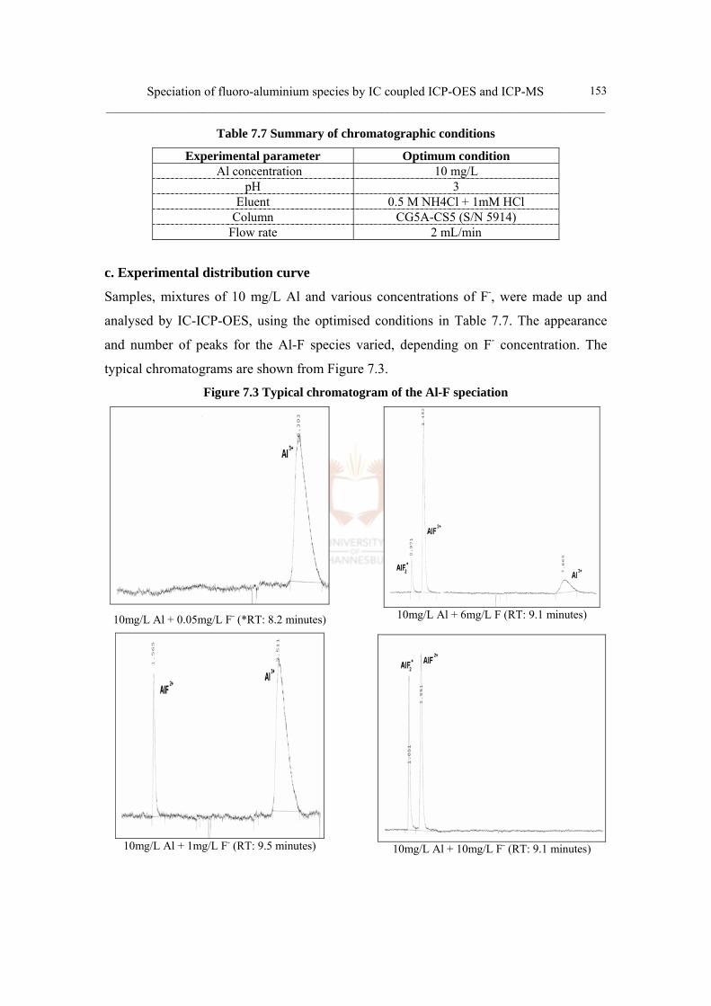
Speciation of fluoro-aluminium species by IC coupled ICP-OES and ICP-MS ______________________________________________________________________________
153
Table 7.7 Summary of chromatographic conditions
Experimental parameter Optimum condition Al concentration 10 mg/L
pH 3 Eluent 0.5 M NH4Cl + 1mM HCl
Column CG5A-CS5 (S/N 5914) Flow rate 2 mL/min
c. Experimental distribution curve
Samples, mixtures of 10 mg/L Al and various concentrations of F-, were made up and
analysed by IC-ICP-OES, using the optimised conditions in Table 7.7. The appearance
and number of peaks for the Al-F species varied, depending on F- concentration. The
typical chromatograms are shown from Figure 7.3.
Figure 7.3 Typical chromatogram of the Al-F speciation
10mg/L Al + 0.05mg/L F- (*RT: 8.2 minutes)
10mg/L Al + 1mg/L F- (RT: 9.5 minutes)
10mg/L Al + 6mg/L F (RT: 9.1 minutes)
10mg/L Al + 10mg/L F- (RT: 9.1 minutes)
Speciation of fluoro-aluminium species by IC coupled ICP-OES and ICP-MS ______________________________________________________________________
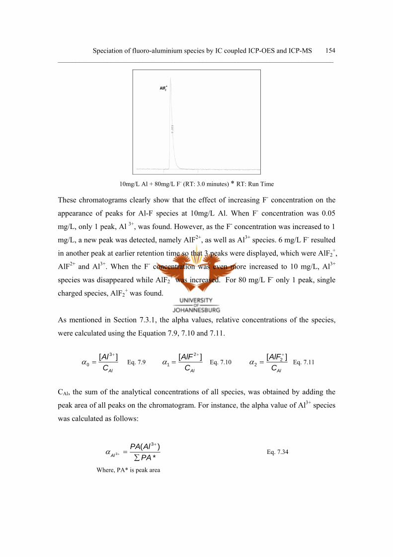
Speciation of fluoro-aluminium species by IC coupled ICP-OES and ICP-MS ______________________________________________________________________________
154
10mg/L Al + 80mg/L F- (RT: 3.0 minutes) * RT: Run Time
These chromatograms clearly show that the effect of increasing F- concentration on the
appearance of peaks for Al-F species at 10mg/L Al. When F- concentration was 0.05
mg/L, only 1 peak, Al 3+, was found. However, as the F- concentration was increased to 1
mg/L, a new peak was detected, namely AlF2+, as well as Al3+ species. 6 mg/L F- resulted
in another peak at earlier retention time so that 3 peaks were displayed, which were AlF2+,
AlF2+ and Al3+. When the F- concentration was even more increased to 10 mg/L, Al3+
species was disappeared while AlF2+ was increased. For 80 mg/L F- only 1 peak, single
charged species, AlF2+ was found.
As mentioned in Section 7.3.1, the alpha values, relative concentrations of the species,
were calculated using the Equation 7.9, 7.10 and 7.11.
AlCAl ][ 3
0
+
=α Eq. 7.9 AlC
AlF ][ 2
1
+
=α Eq. 7.10 AlC
AlF ][ 22
+
=α Eq. 7.11
CAl, the sum of the analytical concentrations of all species, was obtained by adding the
peak area of all peaks on the chromatogram. For instance, the alpha value of Al3+ species
was calculated as follows:
*)( 3
3PAAlPA
Al ∑=
+
+α Eq. 7.34
Where, PA* is peak area
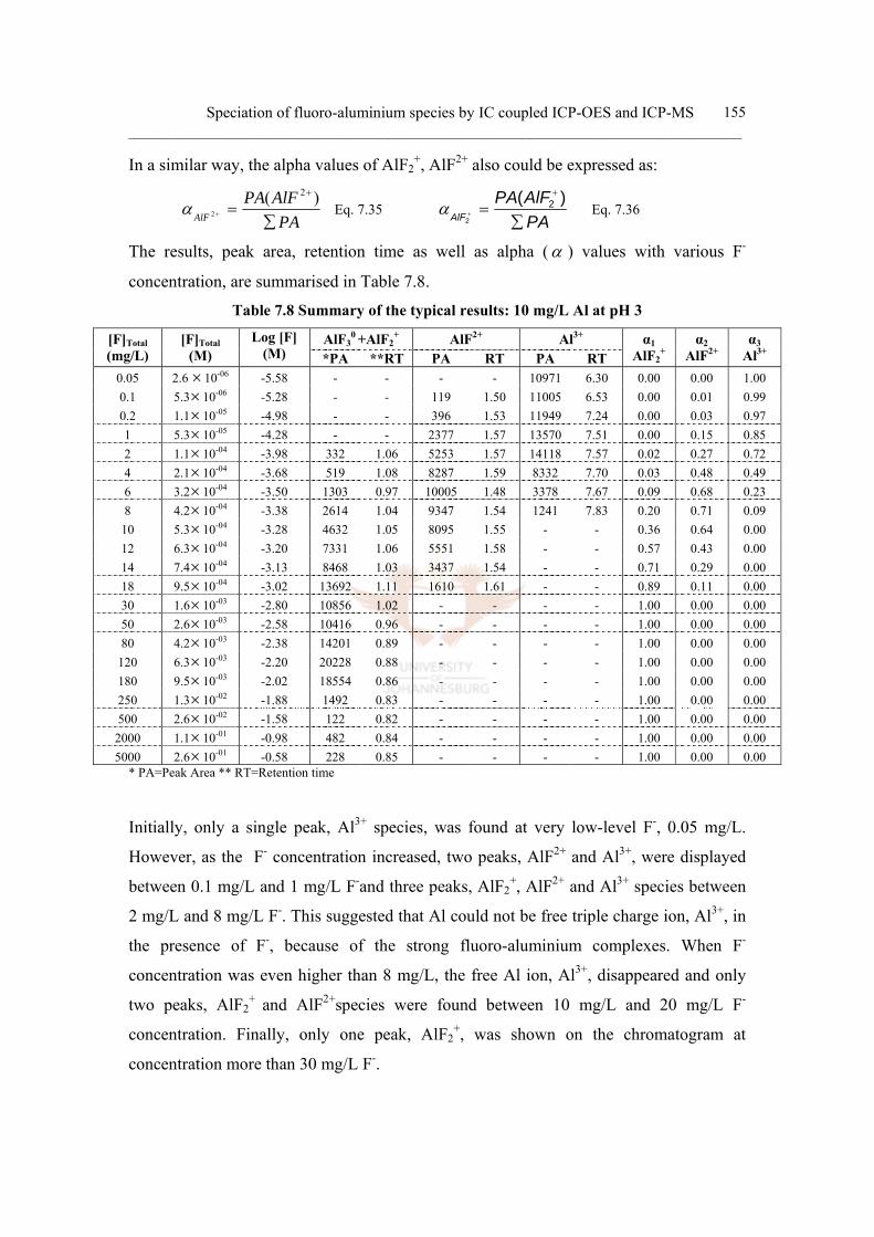
Speciation of fluoro-aluminium species by IC coupled ICP-OES and ICP-MS ______________________________________________________________________________
155
In a similar way, the alpha values of AlF2+, AlF2+ also could be expressed as:
PAAlFPA
AlF ∑=
+
+
)( 2
2α Eq. 7.35 PAAlFPA
AlF ∑=
+
+
)( 22
α Eq. 7.36
The results, peak area, retention time as well as alpha (α ) values with various F-
concentration, are summarised in Table 7.8.
Table 7.8 Summary of the typical results: 10 mg/L Al at pH 3
AlF30 +AlF2
+ AlF2+ Al3+ [F]Total (mg/L)
[F]Total (M)
Log [F] (M) *PA **RT PA RT PA RT
α1 AlF2
+ α2
AlF2+ α3
Al3+ 0.05 2.6 ×10-06 -5.58 - - - - 10971 6.30 0.00 0.00 1.00 0.1 5.3×10-06 -5.28 - - 119 1.50 11005 6.53 0.00 0.01 0.99 0.2 1.1×10-05 -4.98 - - 396 1.53 11949 7.24 0.00 0.03 0.97 1 5.3×10-05 -4.28 - - 2377 1.57 13570 7.51 0.00 0.15 0.85 2 1.1×10-04 -3.98 332 1.06 5253 1.57 14118 7.57 0.02 0.27 0.72 4 2.1×10-04 -3.68 519 1.08 8287 1.59 8332 7.70 0.03 0.48 0.49 6 3.2×10-04 -3.50 1303 0.97 10005 1.48 3378 7.67 0.09 0.68 0.23 8 4.2×10-04 -3.38 2614 1.04 9347 1.54 1241 7.83 0.20 0.71 0.09 10 5.3×10-04 -3.28 4632 1.05 8095 1.55 - - 0.36 0.64 0.00 12 6.3×10-04 -3.20 7331 1.06 5551 1.58 - - 0.57 0.43 0.00 14 7.4×10-04 -3.13 8468 1.03 3437 1.54 - - 0.71 0.29 0.00 18 9.5×10-04 -3.02 13692 1.11 1610 1.61 - - 0.89 0.11 0.00 30 1.6×10-03 -2.80 10856 1.02 - - - - 1.00 0.00 0.00 50 2.6×10-03 -2.58 10416 0.96 - - - - 1.00 0.00 0.00 80 4.2×10-03 -2.38 14201 0.89 - - - - 1.00 0.00 0.00
120 6.3×10-03 -2.20 20228 0.88 - - - - 1.00 0.00 0.00 180 9.5×10-03 -2.02 18554 0.86 - - - - 1.00 0.00 0.00 250 1.3×10-02 -1.88 1492 0.83 - - - - 1.00 0.00 0.00 500 2.6×10-02 -1.58 122 0.82 - - - - 1.00 0.00 0.00 2000 1.1×10-01 -0.98 482 0.84 - - - - 1.00 0.00 0.00 5000 2.6×10-01 -0.58 228 0.85 - - - - 1.00 0.00 0.00
* PA=Peak Area ** RT=Retention time
Initially, only a single peak, Al3+ species, was found at very low-level F-, 0.05 mg/L.
However, as the F- concentration increased, two peaks, AlF2+ and Al3+, were displayed
between 0.1 mg/L and 1 mg/L F-and three peaks, AlF2+, AlF2+ and Al3+ species between
2 mg/L and 8 mg/L F-. This suggested that Al could not be free triple charge ion, Al3+, in
the presence of F-, because of the strong fluoro-aluminium complexes. When F-
concentration was even higher than 8 mg/L, the free Al ion, Al3+, disappeared and only
two peaks, AlF2+ and AlF2+species were found between 10 mg/L and 20 mg/L F-
concentration. Finally, only one peak, AlF2+, was shown on the chromatogram at
concentration more than 30 mg/L F-.
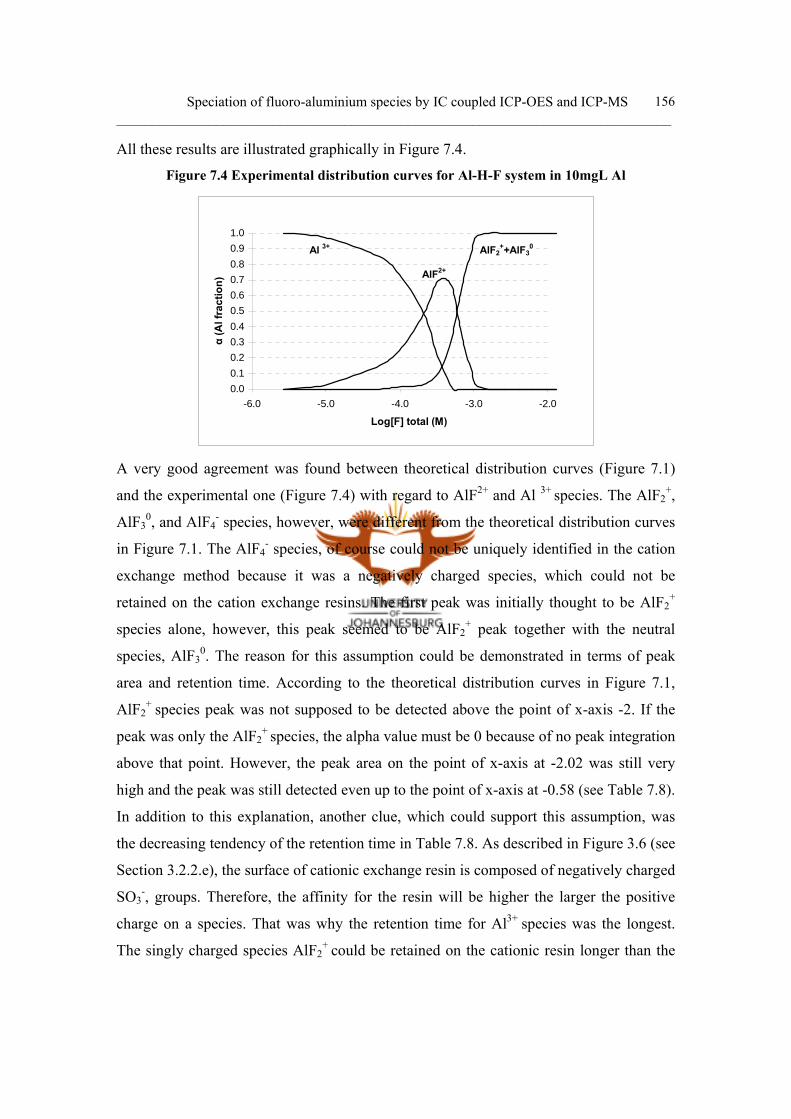
Speciation of fluoro-aluminium species by IC coupled ICP-OES and ICP-MS ______________________________________________________________________________
156
All these results are illustrated graphically in Figure 7.4.
Figure 7.4 Experimental distribution curves for Al-H-F system in 10mgL Al
0.00.10.20.30.40.50.60.70.80.91.0
-6.0 -5.0 -4.0 -3.0 -2.0
Log[F] total (M)
α (A
l fra
ctio
n)
Al 3+
AlF2+
AlF2++AlF3
0
A very good agreement was found between theoretical distribution curves (Figure 7.1)
and the experimental one (Figure 7.4) with regard to AlF2+ and Al 3+ species. The AlF2+,
AlF30, and AlF4
- species, however, were different from the theoretical distribution curves
in Figure 7.1. The AlF4- species, of course could not be uniquely identified in the cation
exchange method because it was a negatively charged species, which could not be
retained on the cation exchange resins. The first peak was initially thought to be AlF2+
species alone, however, this peak seemed to be AlF2+ peak together with the neutral
species, AlF30. The reason for this assumption could be demonstrated in terms of peak
area and retention time. According to the theoretical distribution curves in Figure 7.1,
AlF2+ species peak was not supposed to be detected above the point of x-axis -2. If the
peak was only the AlF2+ species, the alpha value must be 0 because of no peak integration
above that point. However, the peak area on the point of x-axis at -2.02 was still very
high and the peak was still detected even up to the point of x-axis at -0.58 (see Table 7.8).
In addition to this explanation, another clue, which could support this assumption, was
the decreasing tendency of the retention time in Table 7.8. As described in Figure 3.6 (see
Section 3.2.2.e), the surface of cationic exchange resin is composed of negatively charged
SO3-, groups. Therefore, the affinity for the resin will be higher the larger the positive
charge on a species. That was why the retention time for Al3+ species was the longest.
The singly charged species AlF2+ could be retained on the cationic resin longer than the
Speciation of fluoro-aluminium species by IC coupled ICP-OES and ICP-MS ______________________________________________________________________________
157
neutral species, AlF30. In other words, the neutral species, AlF3
0, seemed to be eluted a
little bit earlier than the singly charged species, AlF2+. A good correspondence between
this explanation and the data of retention time for the first peak was found. Therefore, the
first peak was not only AlF2+ species but also AlF2
+ together with AlF30 species.
Concerning this first peak, Hara et al. (2001) also demonstrated that the first peak
represents species with a negative, neutral or 1+ charge. According to the current
experiment, this column system could not separate the neutral and singly charge species
perfectly. Therefore, the distribution curve shown in Figure 7.4, which was drawn for
high F- concentration, depicts AlF2+ together with AlF3
0 species.
7.4.5 Conclusion
Speciation of fluoro-aluminium complexes has been demonstrated using a cation
chromatographic column system, CG5A in conjunction with CS5, coupled to an ICP-
OES as the detector. The species, Al 3+, AlF2+ and possibly, AlF2+ together with the
neutral AlF3,0
were well resolved with this column system and the experimental
distribution curves correlate well with theoretical curves, obtained by calculation from
the complexation constants.
7.5 Anion chromatography – ICP-OES: experimental 7.5.1 Introduction
The purpose of the current work was to develop a speciation method of the mixed
complexes, Al(OH)2F2- and AlF4
-. This was to be carried out using a hyphenated
technique between anion chromatography and inductively coupled plasma-optical
emission spectrometry (IC-ICP-OES). No literature was found on this matter. The
development of a method using an anion exchange chromatographic method was to be
considered. Because of the fact that it would be performed under basic conditions, meant
that it had the risk of blocking the column due to aluminium hydroxide precipitation.
Speciation of fluoro-aluminium species by IC coupled ICP-OES and ICP-MS ______________________________________________________________________________
158
7.5.2 Instrumentation
A Dionex Gradient Pump equipped with a Rheodyne Model 9126 Injection Valve (100
µL sample loop) was coupled to a Dionex Ion Pac AG 5 and AG 14 anion exchange
column. The chromatographic columns were connected to a Varian Liberty 110 ICP
Emission Spectrometer. The flow rate was 1.5 mL/min. Data capturing and peak analyses
were performed with the use of Star Chromatography Software (1995, Varian Associates
Inc.)
7.5.3 Reagents and standard solutions
All reagents were of AR grade and high quality deionised water (18 MΩ) was used for
preparing all solutions. Samples and eluent were filtered through 0.22 µm membrane
filters.
The following solutions were prepared:
• 1000 mg/L Al stock solution: 0.894 g AlCl3·6H2O was dissolved in deionised water
and diluted to 100 mL in a volumetric flask.
• 1000 mg/L F- Stock solution: 0.221 g NaF was dissolved in deionised water and
diluted to 100 mL in a polystyrene volumetric flask.
• Eluent (1mM HCO3-, 3.5mM CO3
2-): 4 mL 0.5 M HCO3-, 14 mL 0.5 M CO3
2-
solutions were combined and diluted to 2000mL.
- 0.5 M CO32- stock solution: 26.49 g Na2CO3 (AnalaR, BDH Chemicals Ltd,
Poole, England) was dissolved in 500 mL deionised water.
- 0.5 M HCO3- stock solution: 21g NaHCO3 (Saarchem (Pty) Ltd) was dissolved
in 500mL deionised water.
• A series of synthetic sample mixtures, 10 mg/L Al and various concentration of F-,
were prepared by the appropriate dilution of the stock solutions adjusted the pH at 9
using NaOH.
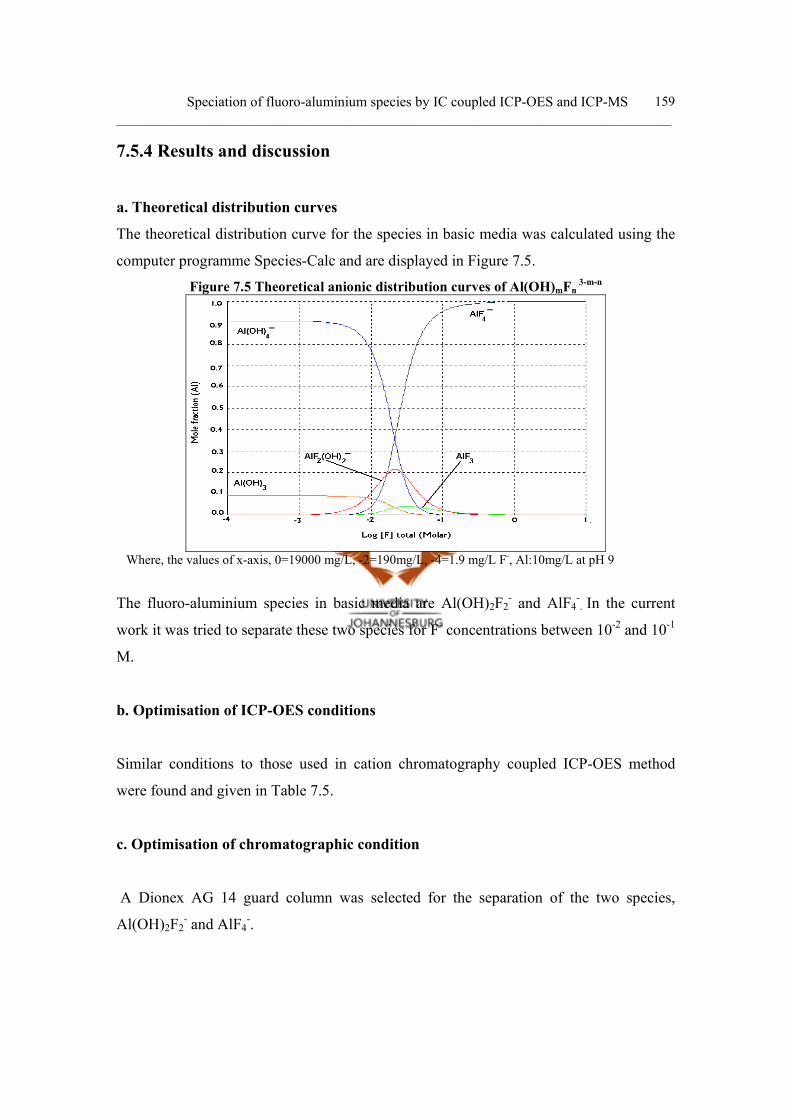
Speciation of fluoro-aluminium species by IC coupled ICP-OES and ICP-MS ______________________________________________________________________________
159
7.5.4 Results and discussion
a. Theoretical distribution curves
The theoretical distribution curve for the species in basic media was calculated using the
computer programme Species-Calc and are displayed in Figure 7.5.
Figure 7.5 Theoretical anionic distribution curves of Al(OH)mFn 3-m-n
Where, the values of x-axis, 0=19000 mg/L, -2=190mg/L, -4=1.9 mg/L F-, Al:10mg/L at pH 9
The fluoro-aluminium species in basic media are Al(OH)2F2- and AlF4
-. In the current
work it was tried to separate these two species for F- concentrations between 10-2 and 10-1
M.
b. Optimisation of ICP-OES conditions
Similar conditions to those used in cation chromatography coupled ICP-OES method
were found and given in Table 7.5.
c. Optimisation of chromatographic condition
A Dionex AG 14 guard column was selected for the separation of the two species,
Al(OH)2F2- and AlF4
-.
Speciation of fluoro-aluminium species by IC coupled ICP-OES and ICP-MS ______________________________________________________________________________
160
10-1M NaOH solution was initially selected to elute the species at the flow rate 2.0
mL/min. However, no peak was detected with this eluent, so it was thought that this
eluent was too weak to elute the species. Thus, sodium bicarbonate/carbonate solution,
which is a stronger eluent, and is the typical eluent for anion chromatographic separations,
was selected as the eluent A single peak was detected at a F- concentration 250 mg/L, at
which two peaks were expected.
To find a column, that was appropriate for separating the two peaks, the AG 5 guard
column was evaluated. Only one peak was obtained as before. This was probably because
the two species had the same single-charge as well as about the same size and thus the
affinity of these two species for the stationary phase seemed to be very similar. This
made the anion separation impossible with the columns tried in this investigation. Owing
to this fact as well as the risk of blocking the columns by aluminium-hydroxide
precipitation, this separation work was discontinued.
7.5.5 Conclusion
An anionic chromatographic procedure with ICP-OES detection was investigated for the
simultaneous separation and determination of Al(OH)2F2- and AlF4
-. However, it was
discontinued because the two species had the same charge and the similar size, which
made separation impossible with the column available in this study.
7.6 Cation chromatography – ICP-MS: experimental 7.6.1 Introduction The cationic fluoro-aluminium speciation, Al 3+, AlF2+ and possibly, AlF2
+ together with
the neutral AlF3, has been demonstrated at 10 mg/L Al concentration, using ICP-OES
detector in Section 7.4. Using this method, all the species, were well resolved and the
comparison with theoretical curves gave results consistent with the experimental
distribution curves. However, the concentration used in ICP-OES detection, 10 mg/L Al,
Speciation of fluoro-aluminium species by IC coupled ICP-OES and ICP-MS ______________________________________________________________________________
161
was quite high compared to the environmental Al concentration level. Thus, the Al-F
speciation using ICP-MS detection, which provides very low detection limit, as described
in Section 3.4.1, was investigated at low level of Al and especially tried to find the 3
peaks configuration.
7.6.2 Instrumentation
A Dionex Gradient Pump equipped with a Rheodyne Model 9126 Injection Valve (100
µL sample loop) was coupled to a Dionex Ion Pac CG5A and CG 5 (Serial number 5914)
cation exchange column. Al-specific ICP-MS detection was carried out using a Thermo
Elemental X 7 (Thermo electron corporation, USA) fitted with a concentric nebuliser
(conical) and a Peltier cooled (2°C) spray chamber (Impact bead type). All
chromatograms were obtained monitoring Al at m/z 27 using time resolved analysis. The
flow rate was 2 mL/min. Thermo electron Plasma Lab software was used for system
control and data collection.
7.6.3 Reagents and standard solutions
All reagents were of AR grade, ultra-pure HNO3 (Merck), which contain no Al impurity,
and deionised water (18 MΩ cm), obtained from a combination MilliQ Elix and Milli Q-
element water purification system, was used for preparing all solutions. Samples and
eluent were filtered through 0.22 µm membrane filters.
The following solutions were prepared:
• 1000 mg/L Al stock solution: Dissolve 0.894 g AlCl3·6H2O in deionised water
and dilute to 100 mL in a volumetric flask.
• 1000 mg/L F- Stock solution: Dissolve 0.221 g NaF in deionised water and dilute
to 100 mL in a polystyrene volumetric flask.
• Eluent (0.5 M NH4NO3, 1mM HNO3): Dissolve 40.02 g NH4NO3 in deionised
water and dilute to 1L with a 1 mM HNO3 matrix (10mL of 0.1M HNO3) in a
volumetric flask.
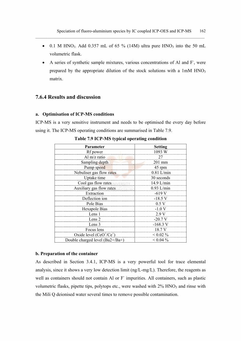
Speciation of fluoro-aluminium species by IC coupled ICP-OES and ICP-MS ______________________________________________________________________________
162
• 0.1 M HNO3: Add 0.357 mL of 65 % (14M) ultra pure HNO3 into the 50 mL
volumetric flask.
• A series of synthetic sample mixtures, various concentrations of Al and F-, were
prepared by the appropriate dilution of the stock solutions with a 1mM HNO3
matrix.
7.6.4 Results and discussion
a. Optimisation of ICP-MS conditions
ICP-MS is a very sensitive instrument and needs to be optimised the every day before
using it. The ICP-MS operating conditions are summarised in Table 7.9.
Table 7.9 ICP-MS typical operating condition
Parameter Setting Rf power 1093 W
Al m/z ratio 27 Sampling depth 201 mm
Pump speed 45 rpm Nebuliser gas flow rates 0.81 L/min
Uptake time 30 seconds Cool gas flow rates 14.9 L/min
Auxiliary gas flow rates 0.93 L/min Extraction -619 V
Deflection ion -18.5 V Pole Bias 0.5 V
Hexapole Bias -1.0 V Lens 1 2.9 V Lens 2 -20.7 V Lens 3 -168.3 V
Focus lens 18.7 V Oxide level (CeO+/Ce+) < 0.02 %
Double charged level (Ba2+/Ba+) < 0.04 %
b. Preparation of the container
As described in Section 3.4.1, ICP-MS is a very powerful tool for trace elemental
analysis, since it shows a very low detection limit (ng/L-mg/L). Therefore, the reagents as
well as containers should not contain Al or F- impurities. All containers, such as plastic
volumetric flasks, pipette tips, polytops etc., were washed with 2% HNO3 and rinse with
the Mili Q deionised water several times to remove possible contamination.
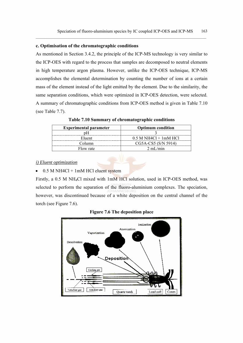
Speciation of fluoro-aluminium species by IC coupled ICP-OES and ICP-MS ______________________________________________________________________________
163
c. Optimisation of the chromatographic conditions
As mentioned in Section 3.4.2, the principle of the ICP-MS technology is very similar to
the ICP-OES with regard to the process that samples are decomposed to neutral elements
in high temperature argon plasma. However, unlike the ICP-OES technique, ICP-MS
accomplishes the elemental determination by counting the number of ions at a certain
mass of the element instead of the light emitted by the element. Due to the similarity, the
same separation conditions, which were optimized in ICP-OES detection, were selected.
A summary of chromatographic conditions from ICP-OES method is given in Table 7.10
(see Table 7.7).
Table 7.10 Summary of chromatographic conditions
Experimental parameter Optimum condition pH 3
Eluent 0.5 M NH4Cl + 1mM HCl Column CG5A-CS5 (S/N 5914)
Flow rate 2 mL/min
i) Eluent optimization
• 0.5 M NH4Cl + 1mM HCl eluent system
Firstly, a 0.5 M NH4Cl mixed with 1mM HCl solution, used in ICP-OES method, was
selected to perform the separation of the fluoro-aluminium complexes. The speciation,
however, was discontinued because of a white deposition on the central channel of the
torch (see Figure 7.6).
Figure 7.6 The deposition place

Speciation of fluoro-aluminium species by IC coupled ICP-OES and ICP-MS ______________________________________________________________________________
164
Figure 7.6 clearly shows that the deposition positioned at the place where desolvation
traditionally occurs. This meant that the component of deposition came from the eluent.
Instead of using 0.5M ammonium chloride, lower concentrations of ammonium chloride,
such as 0.2M, 0.3M and 0.4M, were tested, however, these also yielded the deposition.
Thus, ammonium chloride eluent could not be used in further work.
• 0.45M HNO3 eluent system
Bayón et al. (1999) stated that saline solutions, such as K2SO4, are not recommended in
ICP-MS, because of the possibility of clogging the central channel of the torch and
deposits on the cones. 0.45 M nitric acid, using CG 2 guard column, was selected to
separate the two species, AlF2+ and Al3+. Although only two species were shown in this
paper and the pH was lower than 3, which was the optimized value in the current work,
this eluent was tested to separate the 3 peaks in the current experiment. However, only 2
peaks were found on the chromatogram using nitric acid eluent. This meant that H+ alone,
involved in the process of exchange on the resin, was not strong enough to elute 3 fluoro-
aluminium species, Al3+, AlF2+ and possibly, AlF2+ together with the neutral AlF3.
• 0.5 M NH4NO3 + 1mM HNO3 eluent system
An appropriate eluent, which was stronger than HNO3 and could solve the deposition
problem, was necessary. Ammonium nitrate eluent was tested because all components of
the eluent would be converted into the gaseous state in the plasma and so deposition
should be minimal. This eluent system worked well with the Al-F speciation; however, it
also yielded the deposition problem after instrument being used for a long time. A
possible way to solve this problem was to use the 2% HNO3 solution between sample
measurements, which could prevent the high concentration eluent from flowing through
the entire ICP-MS system. This eluent system was better than the ammonium chloride
eluent in terms of preventing blocking the central channel of torch; therefore this eluent
was introduced for further Al-F speciation work.
d. Typical chromatogram
Samples, mixtures of various concentrations of Al and various concentrations of F-, were
made up and analysed by Ion chromatography coupled ICP-MS, using the optimised ICP-

Speciation of fluoro-aluminium species by IC coupled ICP-OES and ICP-MS ______________________________________________________________________________
165
MS conditions in Table 7.9, IC conditions in Table 7.7 with ammonium nitrate eluent
system. This method worked well for Al-F speciation and the typical chromatogram,
having 3 peaks, is shown in Figure 7.7.
Figure 7.7 Typical chromatogram of the Al-F speciation
using ICP MS detector
e. Pitfall of this method
Although the Al-F speciation at low levels could be performed successfully with this
method, deposit formation in the torch after extended use could occur. This required
regular cleaning of the torch.
7.6.5 Conclusion
The speciation of Al-F was done by using a cation chromatographic column system,
CG5A in conjunction with CS5, coupled to an ICP-MS or ICP-OES as the detector. The
species, Al 3+, AlF2+ and possibly, AlF2+ together with the neutral AlF3,
0 were well
resolved with this column system and the ammonium nitrate eluent system.
Conclusion _____________________________________________________________________________
166
Chapter 8 Conclusion
The investigation of the chemistry and analytical chemistry of low-level (0.05 – 1
mg/L) F- determination was intensively discussed in this thesis. Method validation and
the development of standard ISE and IC procedures for the determination of low-level
F- in deionised water brought new insights in the requirements for accurate analytical
procedures for F- (Chapter 4). It was found that ISE gave more accurate and precise
results. Therefore, ISE is recommended for low level F- determination. In Chapter 5, the
procedures for using ISE and IC determinations, developed in Chapter 4, were evaluated
for the analysis of natural waters. The % recoveries of laboratory fortified samples
(LFM) samples were within the acceptable criterion (75-120 %) as described in the U.S.
EPA method 300.1. The % recovery obtained by the ISE method showed better
accuracy than that by the IC method and the IC method was more susceptible by the
influence of the matrix. Therefore, overall the ISE methodology was found to be
preferable for the accurate determination of F- in both deionised water and natural water
sample matrices.
An Inter-laboratory study in conjunction with SABS (Chapter 6) showed that the ISE
method is the most commonly used method in South African laboratories for
determination of F-. The best accuracy, calculated from average absolute Z-scores, was
achieved by using ISE methodology. This result supported the conclusion from Chapter
4 and Chapter 5. The proficiency of the procedures developed in this study was proven
through the best results obtained by Lab X (UJ Analytical chemistry lab), which
obtained the most accurate results among 66 participants in South Africa laboratories.
The speciation of cationic fluoro-aluminium complexes, Al 3+, AlF2+ and, AlF2+
together with the neutral AlF30, has been successfully accomplished using a cation

Conclusion _____________________________________________________________________________
167
chromatographic column system coupled to an ICP-OES or ICP-MS. The experimental
distribution curves at 10mg/L Al concentration level, achieved by the developed method,
IC-ICP-OES with ammonium chloride eluent system, correlated well with theoretical
curves, obtained by calculation from the complexation constants. However, the
separation and determination of Al(OH)2F2- and AlF4
- , an anionic chromatographic
procedure with ICP-OES detection, was found impossible because the two species had
the same charge (-1) and the similar size.
References ______________________________________________________________________________
168
References
1. ALEXANDERSEN P, RIIS BJ and CHRISTIANSEN C (1999)
Monofluorophosphate combined with hormone replacement therapy induce a
synergistic effect on bone mass by dissociating bone formation and resorption in
postmenopausal women: a randomized study. J. Clin. Endocrinol Metab. 84 2013-
3020
2. ALPÍZAR J, CRESPÍ A, CLADERA A, FORTEZA R and CERDÁ V (1996)
Simultaneous determination of chloride and fluoride ions in waters by sequential
injection analysis electroanalysis 8 1051-1054
3. ANALYTICAL WORKING GROUP OF THE COMITÉ TECHNIQUE EUROPÉEN
DU FLUOR (1986) The determination of fluoride in environmentally relevant
matrices Analytica Chimica Acta 182 1-16
4. Annual Book of ASTM Standards Part 31, “Water”, Standard D 1179-72, Method A,
(1976) Am. Soc. Test Master 310
5. BABCOCK RH and JOHNSON KA (1968) Selective ion electrode system for
fluoride analyses. J. Am. Water Works Assoc. 60 953-961
6. BAKER JP and SCHOFIELD CL (1982) Aluminum toxicity to fish in acidic waters.
Water, Air and Soil Pollut. 18 289-309
7. BARNETT NW, JONES P and HANDLEY HW (1993) The use of zirconyl xylenol
orange for the post-column spectroscopic detection of fluoride in ion chromatography
Analytical letters 26 2525-2529
8. BAYLEY TA, HARRISON JE, MURRAY TM, JOSSE RG, STURTRIDGE W,
PRITZKER KP, STRAUSS A, VIETH R and GOODWIN S (1990) Fluoride-induced
fractures: relation to osteogenic effect. J. Bone Miner. Res. 5 (suppl 1): S217-S222
9. BAYÓN MM, GARCIA AR, ALONSO JIG and SANZ-MEDEL A (1999) Indirect
determination of trace amounts of fluoride in natural waters by ion chromatography: a
comparison of on-line post-column fluorimetry and ICP-MS detectors Analyst 124
27-31
10. BELLACK E (1958) Simplified Fluoride Distillation Method J. Am. Water Works
Assoc. 50
References ______________________________________________________________________________
169
11. BELLACK E and SCHOUBOE PJ (1958) Rapid photometric Determination of
Fluoride in Water Anal. Chem. 30 2032
12. BERSCH PM and ANDERSON MA (1989) Speciation of aluminum in aqueous
solutions using ion chromatography Anal. Chem. 61 535-539
13. BONDOUX G and JONES T (1995) Analysis of Anions and cations in deionised
water at parts-per-billion levels LC-GC 13 144-148
14. BORRMANN G and SEUBERT A (1996) Aluminum speciation by liquid
chromatography concerning hydro- and geo-chemical aspects Analytica Chimica
Acta 332 233-239
15. BORZITSKY JA, DVININ A, PETRUKHIN OM and UROSOV YI (1993) Flow
cell with double slope factor for potentiometric determination of fluoride at low
concentrations Analyst 118 859-861
16. BUTLER JN (1969) Ion Selective Electrodes (DURST RA ed.) Chapter 5 National
bureau of standards special publication 314 Washington D.C.
17. BUTLER WJ, SEGRETO V and COLLINS E (1985) Prevalence of dental mottling
in school-aged lifetime residents of 16 Texas communities Am. J. Public health 75
1408-1412
18. CABELLO-TOMAS ML and WEST TS (1969) Kinetochromic spectrophotometry-
I Determination of fluoride by catalysis of the zirconium-xylenol orange reaction
Talanta 16 781-788
19. CARDWELL TJ, CATTRALL RW, HAUSEN PC and HAMILTON IC (1987)
Buffer systems for use with the fluoride electrode in flow injection analysis Anal.
Chem. 59 206-208
20. CHEN XY, LIN MQ, HE ZL, CHEN C, MIN D, LIU YQ and YU MH (1996)
Relationship between total fluoride intake and dental fluorosis in areas polluted by
airborne fluoride. Fluoride 29 7-12
21. CHEN Y, LIN M, HE Z, XIE X, LIU Y, XIAO Y, ZHOU J, FAN U, XIAO Z and
XU F (1993) Air pollution-type fluorosis in the region of Pingxiang, Jiangxi,
People’s Republic of China. Arch. Environ. Health 48 246-249
22. CRAPPER MDR and BONI D (1980) Aluminum in human brains disease-an
overview. Neurotoxicol 1 3-16

References ______________________________________________________________________________
170
23. CROSBY NT, DENNIS AL and STEVENS JG (1968) An evaluation of some
methods for the determination of fluoride in potable waters and other aqueous
solutions Analyst 93 643-652
24. DAVIDSON AM, WALKER GS and LEWINS AM (1982) Water supply
aluminum concentrations, dialysis dementia, and effects of reverse osmosis water
treatment. Lancet. 2 785-787
25. DEAN HT (1934) Classification of mottled enamel diagnosis J. Am. Dent. Assoc.
21 1421-1426
26. DEPARTMENT OF HEALTH (2000) Regulation No. 873 Regulations under the
Health Act, 1977 (Act No. 63 of 1977) Regulations on Fluoridating Water Supplies.
Government Gazette, 8 September 2000, 423 No 21533, Pretoria.
27. DEVINE RF and PARTINGTON GL (1975) Interference of sulfate ion on
SPANDS colorimetric determination of fluoride in wastewaters Environ. Sci.
Technol. 9 678-679
28. DIONEX (1997) PeakNet Software User’s Guide Document No. 034914
29. DIONEX APPLICATION NOTE 42 (1986) Determination of aluminum by ion
chromatography Dionex Corporation Sunnyvale, CA
30. DIONEX APPLICATION NOTE 133 Determination of inorganic anions in
drinking water by ion chromatography Dionex
31. DIONEX APPLICATION NOTE 135 Determination of Inorganic Anions in
Wastewater by Ion Chromatography Dionex
32. DIONEX APPLICATION NOTE 140 Fast Analysis of anions in drinking water by
ion chromatography Dionex
33. DIONEX APPLICATION NOTE 154 Determination of inorganic anions in
environmental waters using a hydroxide-selective column Dionex
34. DOUGLAS DP (1979) Stability Constants of Metal-Ion Complexes Part B:
ORGANIC LIGANDS” IUPAC Chemical Data Series, No. 22. PERGAMON
PRESS, OXFORD, NEW YORK, TORONTO, SYDNEY, PARIS, FRANDFURT
35. DRISCOLL CT and LETTERMAN RD (1988) Chemistry and fate of Al III in
treated drinking water. Int. J. Environ. Eng. Div. 114(1) 21-37
References ______________________________________________________________________________
171
36. DUFF EJ and STUART JL (1975) The successive determination of chloride,
fluoride and sodium in single samples of orthophosphate minerals by means of ion-
selective electrodes Talanta 22 823-826
37. DURRANT PJ and DURRANT B (1970) Sub-group III N boron, aluminum,
indium and thallium In introduction to advanced Inorganic Chemistry, 2nd edn. New
York John Wiley 522-600
38. DURST RA (1969) Determination of fluoride by analyte addition potentiometry.
Microchim. Acta 31 611-614
39. DURST RA (1969) Ion Selective Electrodes National bureau of standards special
publication 314 Washington D.C.
40. ERIK H (1982) Stability Constants of Metal-Ion Complexes Part A: INORGANIC
LIGANDS” IUPAC Chemical Data Series, No 21. PERGAMON PRESS,
OXFORD, NEW YORK, TORONTO, SYDNEY, PARIS, FRANDFURT
41. FANG Z, ZHU Z, ZHANG S, XU S, GUO L and SUN L (1988) On-line separation
and preconcentration in flow injection analysis Analytica Chimica Acta 214 41-55
42. FARAJ-ZADEH MA and KALHOR EG (2001) Extraction-spectrophotometric
method for determination of fluoride in the range of microgram per liter in natural
waters Mikrochim. Acta 137 169-171
43. FEDRAL REGISTER,1991 Jan 30, 56:20:3573
44. FETIEF DH, SUMMERLIN DJ, HARRIS BE, BRADLEY EL (1985) An
evaluation of three procedures for fluoride analysis. Caries Res. 19 248-254
45. FRANT MS and ROSS JW (1968) Use of a total ionic strength adjustment buffer
for electrode determination of fluoride in water supplies. Anal. Chem. 40 1169-1171
46. FRANT MS and ROSS UW (1966) Electrode for sensing fluoride ion activity in
solution. Science 154 1553-1554
47. FRENZEL W and BRÄTTER (1986) Fluoride ion-selective electrode in flow
injection analysis Analytical Chimica Acta 187 1-16
48. FRENZEL W and BRÄTTER P (1986) The fluoride ion-selective electrode in flow
injection analysis: part 3. Application Analytica Chimica Acta 188 151-164
49. FRITZ JS, RICHARD MJ and KARRAKER SK (1958) Potentiometric titrations
with EDTA. Use of masking agents to improve selectivity Anal. Chem. 30 1347-
1350
References ______________________________________________________________________________
172
50. FRY BW and TAVES DR (1970) Serum fluoride analysis with fluoride electrode. J.
Lab. Clin. Med. 756 1020-1025
51. GARDNER MJ and GUNN AM (1991) Bioavailability of Al from food and
drinking water. Proc. Roual Soc. Med. Round Table Series: Alzheimer’s Diseases
and the Environment, London, UK
52. GARRIDO M, LISTA AG, PALOMEQUE M and FERNÁNDEZ BAND BS
(2002) Fluorimetric determination of fluoride in a flow assembly integrated on-line
to an open/closed FIA system to remove interference by solid phase extraction
Talanta 58 849-853
53. HAARHOFF J (2003) The accuracy of fluoride measurement in water and its
implications for water fluoridation (Rapid communication) Water S.A. 29 219-224
54. HALL LL, SMITH FA, DE LOPEZ OH, GARDNER KE (1972) Direct
potentiometric determination of total ionic fluoride in biological fluids. Clin. Chem.
18 1455-1458
55. HALLSWORTH AS, WEATHERELL JA, DAN DEUTSCH D (1976)
Determination of subnanogram amounts of fluoride with the fluoride electrode.
Anal. Chem. 48 1660-1664
56. HARA H and HUANG CC (1997) Buffer composition suitable for determining
very low fluoride concentrations using a fluoride ion-selective electrode and its
application to the continuous analysis of rain water Analytica. Chimica Acta 338
141-147
57. HARWOOD JE (1969) The use of an ion-selective electrode for routine fluoride
analyses on water samples Water Research 3 273-280
58. JACKSON PE (2000) in: MEYERS RA (Editor) Encyclopedia of Analytical
Chemistry John Wiley and Sons Ltd., Chichester 3 2779
59. JACKSON PE (2001) Determination of inorganic ions in drinking water by ion
chromatography trends in analytical chemistry 20 320-329
60. JACKSON PE, WEIGERT C, POHL CA and SAINI C (2000) Determination of
inorganic anions in environmental waters with a hydroxide-selective column
Journal of Chromatography A 884 175-784
61. JAVIS KE, GRAY AL and HOUK RS (1992) Handbook of Inductively Coupled
plasma mass spectrometry Chapman and Hall New York
References ______________________________________________________________________________
173
62. JEKEL MR (1991) Aluminum in water: How it can be removed? Use of aluminum
salts in treatment Proc. of the Int. Water Supply Assoc. Copenhagen, Demark, May
25-31
63. JOACHIM W (1986) Handbook of Ion Chromatography Dionex Corporation
publishers Sunnyvale California
64. JONES P (1991) The investigation of aluminum speciation in natural and potable
water using short-column ion chromatography Int. J. Environ. Anal. Chem. 44 1-10
65. JONES P (1992) Development of a high-sensitivity ion chromatography method for
the determination of trace fluoride in water utilizing the formation of the AlF2+
species Analytica Chimica Acta 258 123-127
66. KATHRYN EML and HOWARD LC (1973) Comparison of the SPANDS-
Zirconium Lake and Specific Ion Electrode Methods of Fluoride Determination in
Stack Emission Samples Anal. Chem. 45, 1272
67. KAURANEN P (1977) The use of buffers in the determination of fluoride by an Ion
Selective Electrode at low concentration s and in the presence of aluminum
Analytical Letters 10 451-465
68. KHALIFA ME and HAFEZ MAH (1998) Spectrophtometric and complexometric
methods for the determination of thorium and fluoride using bromocresol orange
reagent Talanta 47 547-559
69. KISSA E (1987) Determination of inorganic fluoride in blood with a fluoride ion-
selective electrode. Clin.Chem. 332 253-255
70. LAJUNEN LHJ (1991) Spectrochemical Analysis by Atomic Absorption and
Emission, University of Oulu, Finland
71. LETTERMAN RD and DRISCOLL CT (1994) Control of residual aluminum in
filtered water. AWWA RF Report, AWWA, Denver, CO 80235. 1-93
72. LIBERTY (1991) Analytical methods for the Liberty spectrometer system, Varian
Australia Pty.Ltd., publication N0. 85 100938 00
73. LIU Y ed. (1995) Human exposure assessment of fluoride. An international study
within the WHO/UNEP Human Exposure Assessment Location (HEAL)
Programme. Beijing, Chinese Academy of Preventive Medicine, Institute of
Environmental Health Monitoring, Technical Cooperation Centre of
Fluoride/HEAL Programme, 64
References ______________________________________________________________________________
174
74. LOPES DA CONCEIÇÃO AC, CORREIA DOS SANTOS MM, SIMÕES
GONÇALVES and SANTOS FJV (2000) Gradient flow titration for the
determination of fluoride ion in natural waters Talanta 50 1245-1252
75. MAC LEOD KE and CRIST HL (1973) Comparison of the SPANDS-Zirconium
lake and specific ion electrode methods of fluoride determination in stack emission
samples Anal. Chem. 45 1272-1273
76. MARTYN CN, OSMAND C, EDWARDSON JA, BARKER KJP, HARRIS EC
and LACEY RFC (1989) Geotraphical relatioin between Alzheimer’s disease and
aluminum in drinking water. The Lancet. I (8629) 59-62
77. MCCAFFREY LP (1994) Fluoride electrode vs ion chromatographic analysis of
groundwater. Abstract Volume Analytika 94 87
78. MEUNIER PH, SEVERT JL, REGINSTER JY, BRIANCON D, APELBOOM T,
NETTER P, LOEB G, ROUILLON A, BARRY S, EVREUS JC, AVOUAC B and
MARCHANDISE X (1998) Fluoride salts are no better at preventing new vertebral
fractures than calcium-vitamin D in postmenopausal osteoporosis: the FAVO Study.
Osteoporosis Int, 8 4-12
79. MILLER JC and MILLER JN (1993) Statistics for Analytical Chemistry 3 rd Ed.,
Prentice Hall
80. MONSTER A and GOLIGHTLY DW (1992) Inductively Coupled Plasmas in
Analytical Atomic spectrometry 2nd Ed. VCH Publishers Cambridge
81. MOORE GL (1989) Introduction to Inductively coupled plasma atomic emission
spectrometry Elsevier Amsterdam
82. MOSKVIN LN, KATRUZOV AN and NIKITINA TG (1998) Ion-chromatographic
determination of fluoride and chloride ions in high-purity water Journal of Anal.
Chem. 53 173-177
83. MOTELLIER S and PITSCH H (1994) Determination of aluminum and its fluoro
complexes in natural waters by ion chromatography Journal of Chromatography A
660 211-217
84. MURRY JJ, RUGG0GUNN AJ and JENKINS GN (1991) Fluorides in Caries
Prevention (3rd edn.). Butterworth-Heineman Ltd, Oxford
85. NAJIB FM and OTHMAN S (1992) Computer-aided flow-analysis for laboratory
use and process analysis. Anal. Instrum. 20 79-100

References ______________________________________________________________________________
175
86. NAKAJIMA H, KOMATSU H and OKABE T (1997) Aluminum ions in analysis
of released fluoride from glass ionomers. Journal of Dentistry 25 137-144
87. NICHOLSON K and DUFF EJ (1981) Fluoride determination in water: An
optimum buffer system for use with the fluoride-selective electrode Analytical
letters 14(A7) 493-517
88. NICO (2000) Guide to ISE measurements, www.nico2000.net (accessed May/2004)
89. NILSON R (1990) Residual aluminum concentration in the drinking water after
treatment with aluminum or iron salts. In: HH Hahn and R Klute(eds.) Chemical
Water and Wastewater Treatment, Springer-Verlag, Berlin, Germany. 329-410
90. NISHIMOTO J, YAMADA T and TABATA M (2001) Solvent extraction and
fluorometric determination of fluoride ion at ppb level in the presence of large
excess of aluminum (III) and iron (III) by using an expanded porphyrin, sapphyrin
Analytica Chimica Acta 428 201-208
91. OKAMOTO Y (2001) Determination of fluorine in aqueous samples by
electrothermal vaporization inductively coupled plasma mass spectrometry (ETV-
ICP-MS). J. Anal. At. Spectrom. 16 539-541
92. OKUTANI T, TANAKA C and YAMAGUCHI Y (1989) Determination of fluoride
in natural waters by ion-selective electrode potentiometry after co-precipitation with
aluminum phosphate Talanta 36 973-976
93. OLESIK JW (1996) Fundamental Research in ICP-OES and ICP-MS Anal. Chem.
68 1996
94. OLIVE RT and CLAYTON AG (1970) Direct determination of fluoride in
miscellaneous fluoride materials with the Orion fluoride electrode Analytica
Chimica Acta 51 409-415
95. ORION (1982) Instruction manual, fluoride electrodes, model 94-09 Orion
Research, Cambridge, MA
96. OSZWALDOWSKI S, LIPKA R, MAJEWSKI T and JAROSZ M (1998) Sensitive
reversed-phase liquid chromatographic determination of fluoride based on its
ternary systems with zirconium (IV) or hafnium (IV) and 2-(5-bromo-2-
pyridylazo)-5-diethylaminophenol Analyst 123 1529-1533
97. PAK CYC, SAKHAEE K, PIZIAK V, PETERSON RD, BRESLAU NA, BOYD P,
POINDEXTER JR, HERZOG J, HEARD-SAKHAEE A, HAYNES S, ADAMS-
References ______________________________________________________________________________
176
HUET B and REISCH JS (1994) Slow-release sodium fluoride in the management
of postmenopausal osteoporosis. A randomised controlled trial. Ann. Intern. Med.
120 625-632
98. PAPAEFATATHIOU J, TENA MT and LUQUE DE CASTRO MD (1995) On-line
pervaporation separation process for the potentiometric determination of fluoride in
dirty samples Analytica Chimica Acta 308 246-252
99. PERKIN ELMER SCIEX instruments. Technical note, The 30-Minute Guide to
ICP-MS ( http://las.perkinelmer.com/content/ApplicationNotes/D-6355A.pdf )
100. PICKERING WF (1986) The effect of hydrolyzed aluminum species in fluoride ion
determinations. Talanta 33 661-664
101. PONTIUS FW (1991) Fluoride regulation and water fluoridation J. AWWA 83
20,22,96
102. PONTIUS FW (1993) NRC determines current fluoride MCL appropriate. Opflow
19 3-4
103. REEVES TG (1994) Water Fluorididation: A Manual For Water Plant Operators.
U. S. Department of Health and Human Services, Centers for Disease Control and
Prevention, Atlanta, Georgia.
104. RICHARD AD (1969) Ion selective electrode Department of commerce National
Bureau of Standards Special Publication 314, Washington, D.C.
105. RICHARD FD and GERALD LP (1975) Interference of Sulfate Ion on SPANDS
Colorimetric Determination of Fluoride in Wastewaters. 9 678
106. RICHARDS LF, WESTMORELAND WW, TASHIRO M, MCKAY CM and
MORRISON TJ (1967) Determination of optimum fluoride levels for community
water supplies in relation to temperature. J. Am. Dent. Assoc. 74 389-397
107. RIGGIS BL (1991) Treatment of osteoporosis with sodium fluoride or parathyroid
hormone. Am. J. Med. 91 37S-41S
108. RIZZOLI R, CHEVALLEY T, SLOSMAN DO and BONJOUR JP (1995) Fluoride
intake from foods, beverages and dentifrice by young children in communities with
negligibly and optimally fluoridated water: a pilot study. Community Dent. Oral
Epidemiol 27 288-297
References ______________________________________________________________________________
177
109. ROBERSON CE and HEM JD (1969) Solubility of aluminum in the presence of
hydroxide, fluoride and sulfate. US Geological Survey Water Supply, Paper 1827-C,
US Government Printing Office, Washington, DC.
110. SAAD B, POK RW, SUJARI ANA and SALEH MI (1998) Analysis of anions and
cations in drinking water samples by capillary ion analysis Food chemistry 61 249-
254
111. SAHA S (1993) Treatment of aqueous effluent for fluoride removal. Water Res. 27
1347-1350
112. SARA R and WÄNNINEN E (1975) Separation and determination of fluoride by
diffusion with hexamethyuldisiloxame and use of a fluoride-sensitive electrode
Talanta 22 1033
113. SCHECHER WD and DRISCOLLCT (1988) An evaluation of equilibrium
calculations within acidification models: The effect of uncertainty in measured
chemical components. Water Resour. Res. 24 533-542
114. SKOOG DA, NIEMAN TA and HOLLER FJ (1998) Principles of Instrumental
Analysis, 5th Ed., Harcourt Brace College Publishers, USA
115. SKOOG DA, WEST DM and HOLLER FJ (1997) Fundamentals of Analytical
Chemistry, 7th Ed., Saunders college Publishers, USA
116. SLANINA J, LINERAK WA and BAKKER F (1980) The use of ion-selective
electrodes in manual and computer-controlled flow injection systems Analytica
Chimica Acta 117 91-98
117. SRINIVASAN K and RECHNITZ GA (1988) Reaction rate measurements with
fluoride ion-selective membrane electrode. Formation kinetics of ferrous fluoride
and aluminum fluoride complexes Anal. Chem. 40 1818-1825
118. SRINIVASAN PT, VIRARAGHAVAN T and SUBRAMANIAN KS (1999)
Aluminum in drinking water: An overview. Water S.A. 25(1) 47-55
119. STANDARD METHODS FOR THE EXAMINATION OF WATER AND
WASTEWATER METHOD NO. 414A, Preliminary Distillation Step 389-390 and
Method 414C SPANDS 14th Edition (1975) American Public Health Association,
Washington 393-394
References ______________________________________________________________________________
178
120. STANDARD METHODS FOR THE EXAMINATION OF WATER AND
WASTEWATER METHOD 4500 FD 20th ed., (1998) Am. Pub. Health Assoc.
Washington 4-62
121. STANDARD METHODS FOR THE EXAMINATION OF WATER, SEWAGE,
AND INDUSTRIAL WASTE METHOD (1955) 10th ed. Am. Pub. Health Assoc.,
Am. Water Works Assoc., Am. Federation of Sewage and Industrial Wastes New
York 98-107
122. STEFAN RI, VAN STADEN JF and ABOUL-ENEIN HY (1999) Determination of
fluoride in toothpaste, effluent streams and natural and borehole water using a flow
injection system with a fluoride-selective membrane electrode Pharmaceutica Acta
Helvetiae 73 307-310
123. STEFANOVIĆ ŠC, BOLANĆA T and ĆURKOVIĆ L (2001) Simultaneous
determination of six inorganic anions in drinking water by non-suppressed ion
chromatography Journal of chromatography A 918 325-334
124. TROJANOWICZ M and MATUSZEWSKI W (1982) Limitation of linear response
in flow-injection systems with ion-selective electrodes Analytica Chimica Acta 138
71-79
125. TROJANOWICZ M, ALEXANDER PW and HIBBERT DB (1998) Flow-Injection
analysis wit potentiometric detection for the speciation of fluoride and calcium
Analytica Chimica Acta 366 23-33
126. UNDERWOOD EJ (1977) Trace Elements In Human And Animal Nutrition (4th
edn.) Academic Press, New York, San Francisco, London.
127. US EPA 300.0 (1993) The determination of inorganic anions in water by Ion
Chromatography US Environmental Protection Agency, Cincinnati, OH 45268
128. US EPA 300.1 (1997) Determination of inorganic anions in water by Ion
Chromatography Revision 1.0 US Environmental Protection Agency, Cincinnati,
OH 45268
129. US EPA 340.1 Colorimetric, SPANDS with Bellack Distillation” STORET NO.
Total 00951 Dissolved 00950, 1971-Retrieved May/2004 from
http://www.epa.gov/cgi-bin/climage.sh/ima-link/ORD/images/epa-cin8
References ______________________________________________________________________________
179
130. US EPA METHOD 13A Determination of total fluoride emissions from stationary
sources-SPANDS ZIRCONIUM LAKE METHOD-Retrieved May/2004 from
www.epa.gov/ttn/emc/promgate/m-13b.pdf
131. US EPA METHOD 13B Determination of total fluoride emissions from stationary
sources(specific ion electrode method)-Retrieved May/2004 from
www.epa.gov/ttn/emc/promgate/m-13b.pdf
132. US EPA (1984) Appendix B to Part 136- Definition and Procedure for the
Determination of the Method Detection Limit-Revision 1.11, Federal Register
49(209), 43430, October 26
133. VAN OORT WJ and VAN EERD EJJM (1983) Effect of polishing the fluoride-
selective electrode on the response time and sensitivity in flow systems Analytica
Chimica Acta 155 21-27
134. VAN STADEN JF, STEFAN F and VIRGHILA S (2000) Evaluation of different
SIA sample-buffer configurations using a fluoride-selective membrane electrode as
detector Talanta 52 3-11
135. VAN WYK PJ (1995) Personal communication. Department of Health, Pretoria
136. VANLENGENHAGHE C, VALENSI G and POURBAIX M (1966) Fluorine. In:
Pourbaix m, ed. Atlas of Electrochemical Equilibria in Aqueous Solutions Oxford
Pergamon Press 579-589
137. VARMA A (1991) Handbook of Inductively Coupled plasma atomic emission
Spectroscopy, CRC Press , Florida
138. VICKERY B and VICKERY ML (1976) Suppression of interfering ions in the
analysis of plants to determine fluoride using the fluoride ion selective electrode
Analyst 101 445-454
139. VILLA AE (1988) Rapid method for determination very low fluoride concentration
using an ion-selective electrode. Analyst 113 1299-1303
140. VOGEL GL, CAREY CM, CHOW LC, EKSTRAND J (1990) Fluoride analysis in
nanoliter and microliter-size fluid samples. J. Dent. Res. 69 (special issue) 522-528
141. WADA H, MORI H and NAKAGAWA G (1985) Spectrophotometric
determination of fluoride with lanthanum/alizarin complexone by flow injection
analysis Analytica Chimica Acta 172 297-302
References ______________________________________________________________________________
180
142. WANG H, ZHANG Z, SUN A, LIU D and LIU R (1996) Stopped-flow kinetic
determination of aluminum in Chinese tea leaves by fluoride ion-selective electrode
potentiometry Talanta 43 2067-2072
143. WANG XD, SHEN W, CATTRALL RW, NYBERG GL and LIESEGANG J
(1995) An extrapolation method for the fast evaluation of the fluoride Ion Selective
Electrode equilibrium potential in continuous flow analysis Electroanalysis 7 221-
224
144. WEISS J (1986) Handbook of Ion Chromatography Dionex Corporation California
145. WEISS J, REINHARD S, POHL C, SAINI C and NARAYARAN L (1995)
Stationary phase for the determination of fluoride and other inorganic anions
Journal of chromatography A 706 81-92
146. WELLS AF (1975) Complex, oxy- and hydroxyl-halides. In: Structural Inorganic
Chemistry. 4th edn. London: Oxford University Press 377-413
147. WHO ENVIRONMENTAL HEALTH CRITERIA (1984) Fluorine and fluorides
148. WHO ENVIRONMENTAL HEALTH CRITERIA 227 (2002) Fluorides Geneva
149. WILLET IR (1989) Direct Determination of Aluminum and its Cationic Fluoro-
Complexes by Ion Chromatography Soil Sci. Soc. Am. J. 53 1385-1391
150. WOLFGANG F and PETER B (1986) Fluoride ion-selective electrode in flow
injection analysis Analytical Chimica Acta 187 1-16
151. YUCHI A, MURASE H and WADA H (1995) Structural Features of Organic
Reagents Suitable for Spectrophotometric or Fluorometric Determination of
Fluoride Based on Mixed-Ligand Complex Formation Analytical Sciences 11 221-
226