Evaluation of Advanced Signal Processing Techniques to

ORNL/TM-2016/482

Evaluation of Advanced Signal Processing Techniques to Improve Detection and Identification of Embedded Defects

Dwight Clayton Hector Santos-Villalobos Justin Baba

September 2016

Approved for public release. Distribution is unlimited.

DOCUMENT AVAILABILITY Reports produced after January 1, 1996, are generally available free via US Department of Energy (DOE) SciTech Connect. Website http://www.osti.gov/scitech/ Reports produced before January 1, 1996, may be purchased by members of the public from the following source: National Technical Information Service 5285 Port Royal Road Springfield, VA 22161 Telephone 703-605-6000 (1-800-553-6847) TDD 703-487-4639 Fax 703-605-6900 E-mail [email protected] Website http://www.ntis.gov/help/ordermethods.aspx Reports are available to DOE employees, DOE contractors, Energy Technology Data Exchange representatives, and International Nuclear Information System representatives from the following source: Office of Scientific and Technical Information PO Box 62 Oak Ridge, TN 37831 Telephone 865-576-8401 Fax 865-576-5728 E-mail [email protected] Website http://www.osti.gov/contact.html

This report was prepared as an account of work sponsored by an agency of the United States Government. Neither the United States Government nor any agency thereof, nor any of their employees, makes any warranty, express or implied, or assumes any legal liability or responsibility for the accuracy, completeness, or usefulness of any information, apparatus, product, or process disclosed, or represents that its use would not infringe privately owned rights. Reference herein to any specific commercial product, process, or service by trade name, trademark, manufacturer, or otherwise, does not necessarily constitute or imply its endorsement, recommendation, or favoring by the United States Government or any agency thereof. The views and opinions of authors expressed herein do not necessarily state or reflect those of the United States Government or any agency thereof.

ORNL/TM-2016/482

Electronics and Electrical Systems Research Division

EVALUATION OF ADVANCED SIGNAL PROCESSING TECHNIQUES TO IMPROVE DETECTION AND IDENTIFICATION OF EMBEDDED DEFECTS

Dwight Clayton Hector Santos-Villalobos

Justin Baba

Date Published: September 2016

Prepared by OAK RIDGE NATIONAL LABORATORY

Oak Ridge, Tennessee 37831-6283 managed by

UT-BATTELLE, LLC for the

US DEPARTMENT OF ENERGY under contract DE-AC05-00OR22725

iii

CCONTENTS

Page

LIST OF FIGURES .......................................................................................................................................vLIST OF TABLES ...................................................................................................................................... viiACRONYMS ............................................................................................................................................... ixACKNOWLEDGMENTS ........................................................................................................................... xiEXECUTIVE SUMMARY ........................................................................................................................ xiii1. INTRODUCTION ..................................................................................................................................1

1.1 FABRICATED TEST SPECIMEN, CLASSICAL SYNTHETIC APERTURE FOCUSING TECHNIQUE, AND ELASTIC SOUND PROPERTIES ......................................21.1.1 Fabricated Test Specimen ................................................................................................21.1.2 Classical Synthetic Aperture Focusing Technique ..........................................................31.1.3 Elastic Sound Properties ..................................................................................................4

1.2 WAVELET DECOMPOSITION .................................................................................................51.2.1 Wavelets ..........................................................................................................................51.2.2 Wavelet Packet Decomposition .......................................................................................5

2. RECONSTRUCTION OF ASR AND FREEZE THAW SPECIMENS ................................................92.1 WAVELET PACKET DECOMPOSITION RECONSTRUCTION OF ASR AND NON-

ASR SPECIMENS .......................................................................................................................93. MODEL-BASED ITERATIVE RECONSTRUCTION .......................................................................13

3.1 OVERVIEW ...............................................................................................................................133.2 MODEL-BASED ITERATIVE RECONSTRUCTION .............................................................14

3.2.1 Ultrasonic MBIR ...........................................................................................................153.2.2 Forward Model Crosstalk Upgrade ...............................................................................18

3.3 SIMULATED AND EXPERIMENTAL RESULTS .................................................................213.4 MBIR CLOSING REMARKS ...................................................................................................24

4. UNIVERSAL NDE DATASET FRAMEWORK ................................................................................254.1 INTRODUCTION ......................................................................................................................254.2 THICK, REINFORCED CONCRETE NDE WORKFLOW .....................................................264.3 SOFTWARE ARCHITECTURE: A “PLUG-AND-PLAY” MODEL ......................................27

4.3.1 Data Conversion Interface .............................................................................................284.3.2 Reconstruction Interface ................................................................................................304.3.3 Visualization Interface ...................................................................................................32

4.4 ULTRASOUND DATASET SHARING FORMAT .................................................................324.4.1 Overview on the HDF5 Data File Format .....................................................................32

4.5 DATASET FRAMEWORK CLOSING REMARKS ................................................................345. AUTOMATED DETECTION OF ASR IN CONCRETE ...................................................................35

5.1 FREQUENCY DOMAIN METHODS AND CLASSIFICATION FEATURES ......................365.2 MACHINE LEARNING BASED CLASSIFICATION FEATURES/METHODS ...................37

5.2.1 Artificial Neural Network (ANN) Background .............................................................375.2.2 Development of ANN Algorithm/Method for ASR Detection .....................................385.2.3 Extracting meaningful insights from ANN algorithm/method for ASR detection ........41

5.3 AUTOMATED DETECTION OF ASR CLOSING REMARKS ..........................................426. CONCLUSION .....................................................................................................................................437. REFERENCES .....................................................................................................................................45

iv

v

LLIST OF FIGURES

Figure Page 1. Use of SCC to allow for consolidation without affecting simulated defects. ............................................22. Pitch-Catch method illustrated. ..................................................................................................................33. (a) Block diagram of wavelet decomposition and (b) block diagram of a wavelet packet

decomposition. ..........................................................................................................................................64. Our wavelet decomposition. Nodes in blue were completely analyzed. Underlined nodes appear

in Appendix A and B of [15]. ....................................................................................................................75. SAFT reconstructions for ASR damaged and non-ASR damage specimens for wavelet

decomposed data for frequency bandwidth 0 - 500 kHz (Node 0) ...........................................................96. SAFT reconstructions for ASR damaged and non-ASR damage specimens for wavelet

decomposed data for frequency bandwidth 23.4375 – 31.2500 kHz (Node 66). ....................................107. SAFT reconstructions for ASR damaged and non-ASR damage specimens for wavelet

decomposed data for frequency bandwidth 46.8750 – 54.6875 kHz (Node 69) .....................................118. SAFT reconstruction for (a) thin homogeneous and (b) thick non-homogeneous concrete

structure. ..................................................................................................................................................139. Flowchart of a typical MBIR reconstruction algorithm. ........................................................................1510. Illustration of system matrix coefficient amplitudes for two transducers at time 133us. ......................1711. ICD Algorithm. ......................................................................................................................................1812. Illustration of direct arrival signal. .........................................................................................................1913. Artifacts caused by direct arrival signal from SAFT reconstruction. ....................................................1914. ICD algorithm with direct arrival signal cancellation. ...........................................................................2015. Illustration of ultrasound system position relative to specimens. ..........................................................2116. Comparison between SAFT and MBIR from simulated data of a thin steel plate: (a) Ground

Truth, (b) SAFT Reconstruction, (c) MBIR Reconstruction, (d) SAFT Surface Plot, and (e) MBIR Surface Plot. ...............................................................................................................................22

17. Comparison between SAFT and MBIR from simulated data of a thick steel plate: (a) Ground Truth, (b) SAFT Reconstruction, (c) MBIR Reconstruction, (d) SAFT Surface Plot, and (e) MBIR Surface Plot. ...............................................................................................................................22

18. Comparison between SAFT and MBIR from simulated data of a thin long and short steel plates: (a) Ground Truth, (b) SAFT Reconstruction, (c) MBIR Reconstruction, (d) SAFT Surface Plot, and (e) MBIR Surface Plot. ...................................................................................................................23

19. Comparison between SAFT and MBIR from simulated data of a steel point scatters: (a) Ground Truth, (b) SAFT Reconstruction, (c) MBIR Reconstruction, (d) SAFT Surface Plot, and (e) MBIR Surface Plot. ...............................................................................................................................23

20. Real data obtained from a MIRA system with 40 transducers. The specimen is a cement slab with a steal rebar in the center. ..............................................................................................................23

21. Comparison between SAFT and MBIR from real data for a concrete slab with a rebar at the center: (a) Ground Truth, (b) SAFT Reconstruction, (c) MBIR Reconstruction, (d) SAFT Surface Plot, and (e) MBIR Surface Plot. .............................................................................................24

22. Illustration of the NDE workflow. .........................................................................................................2523. Illustration of NDE workflow for a 10-transducer phased array ultrasound system probing a

thick, reinforced concrete specimen. .....................................................................................................2624. Illustration of the "Plug-and-Play" design. ............................................................................................2725. MATLAB Application GUI conversion pane to convert proprietary files to HDF5. ............................2926. Boilerplate Code for a User-Derived Class from the UTD Interface Class. ..........................................2927. Boiler Plate Code for a User-Derived Class from the Algorithm Interface Class. ................................3028. Reconstruction Interface. .......................................................................................................................31

vi

29. Panoramic frequency-banded SAFT reconstructions for linescan8 Dataset: (a) Frequency band “node 0” from 0-500kHz and (b) Frequency band “node 16” from 31.25-62.5 kHz. ...........................32

30. (a) The hierarchical organization of a typical dataset, (b) encoding information about a linescan node. 33

31. Examples of attributes assigned to (a) a specimen group and (b) a leaf linescan dataset. ...................3432. SAFT reconstructions for (a) ASR damaged and (b) non-ASR damage specimens. ............................3533. FFT spectral analysis results of 4 representative cases. .........................................................................3634. Illustration of neuron connections and weights. ....................................................................................3735. Visualization of the implemented network. ...........................................................................................3836. Confusion matrices for the data set in four categories: training set, validation set, testing set, and

total… ....................................................................................................................................................3937. Size of dataset for each of the nine possible probe-space pairings and the ANN prediction

error… ...................................................................................................................................................4038. Weights of each neuron in the network after training on the specified dataset. ....................................4139. Confusion matrices for the dataset in four categories: training set, validation set, testing set, and

total.. ......................................................................................................................................................42

vii

LLIST OF TABLES

Table Page 1. Example configuration file (CSV viewed in spreadsheet program). .......................................................302. Averaged values for all 45 probe pair combinations for the most representative non-ASR and ASR

samples based on HTI-value classification. R=(nASR/ASR). ................................................................363. Averaged values for all 45 probe pair combinations for the most representative non-ASR and ASR

samples based on HTI-value classification .............................................................................................37

viii

ix

AACRONYMS

BIM Born Iterative Method CG Conjugate Gradient CR3 Crystal River Nuclear Plant CS compressed sensing CT Computed Tomography DPC dry point contact EFIT Elastodynamic Finite Integration Technique GD Gradient Descent GPR Ground Penetrating Radar HFIR High Flux Isotope Reactor ICD Iterative Coordinate Descent IRC intensity reflectivity coefficients LWR Light Water Reactor MAP maximum a posteriori MAST Multi-Axial Subassemblage Testing MBIR Model-Based Iterative Reconstruction MLE maximum likelihood estimation NDE Nondestructive evaluation NPP Nuclear power plant NUFFT Non-uniform Fast Fourier Transform ORNL Oak Ridge National Laboratory PCC Portland cement concrete PET positron emission tomography PSF point spread function q-GGMRF q-Generalized Gaussian Markov Random Fields ROI region of interest SAFT Synthetic Aperture Frequency Technique SCC self-consolidating concrete SIRT simultaneous iterative reconstruction technique TV Total Variation UCT ultrasound computed tomography UMN University of Minnesota UMN-TGL University of Minnesota – Theodore V. Galambos Structural Engineering Laboratory

xi

AACKNOWLEDGMENTS

The work is funded by the U.S. Department of Energy’s office of Nuclear Energy under the Light Water Reactor Sustainability (LWRS) program. The authors also want to acknowledge the assistance of our summer interns, Luke Prince, Kelsey Klett, and Joseph Clayton, who helped to make this report possible. Luke worked on the Universal Framework for NDE Ultrasound Datasets. Kelsey worked processing and assessing the reconstruction results. Joseph worked on implementing a machine learning algorithm for the identification of specimens with ASR defects.

xiii

EEXECUTIVE SUMMARY

By the end of 1996, 109 Nuclear Power Plants were operating in the United States, producing 22% of the Nation’s electricity [1]. At present, more than two thirds of these power plants are more than 40 years old. The purpose of the U.S. Department of Energy Office of Nuclear Energy’s Light Water Reactor Sustainability (LWRS) Program is to develop technologies and other solutions that can improve the reliability, sustain the safety, and extend the operating lifetimes of nuclear power plants (NPPs) beyond 60 years [2]. The most important safety structures in an NPP are constructed of concrete. The structures generally do not allow for destructive evaluation and access is limited to one side of the concrete element. Therefore, there is a need for techniques and technologies that can assess the internal health of complex, reinforced concrete structures nondestructively.

Previously, we documented the challenges associated with Non-Destructive Evaluation (NDE) of thick, reinforced concrete sections and prioritized conceptual designs of specimens that could be fabricated to represent NPP concrete structures [3]. Consequently, a 7 feet tall, by 7 feet wide, by 3 feet and 4-inch-thick concrete specimen was constructed with 2.257-inch-and 1-inch-diameter rebar every 6 to 12 inches. In addition, defects were embedded the specimen to assess the performance of existing and future NDE techniques. The defects were designed to give a mix of realistic and controlled defects for assessment of the necessary measures needed to overcome the challenges with more heavily reinforced concrete structures. Information on the embedded defects is documented in [4]. We also documented the superiority of Frequency Banded Decomposition (FBD) Synthetic Aperture Focusing Technique (SAFT) over conventional SAFT when probing defects under deep concrete cover. Improvements include seeing an intensity corresponding to a defect that is either not visible at all in regular, full frequency content SAFT, or an improvement in contrast over conventional SAFT reconstructed images.

This report documents our efforts in four fronts: 1) Comparative study between traditional SAFT and FBD SAFT for concrete specimen with and without Alkali-Silica Reaction (ASR) damage, 2) improvement of our Model-Based Iterative Reconstruction (MBIR) for thick reinforced concrete [5], 3) development of a universal framework for sharing, reconstruction, and visualization of ultrasound NDE datasets, and 4) application of machine learning techniques for automated detection of ASR inside concrete. Our comparative study between FBD and traditional SAFT reconstruction images shows a clear difference between images of ASR and non-ASR specimens. In particular, the left first harmonic shows an increased contrast and sensitivity to ASR damage. For MBIR, we show the superiority of model-based techniques over delay and sum techniques such as SAFT. Improvements include elimination of artifacts caused by direct arrival signals, and increased contrast and Signal to Noise Ratio. For the universal framework, we document a format for data storage based on the HDF5 file format, and also propose a modular Graphic User Interface (GUI) for easy customization of data conversion, reconstruction, and visualization routines. Finally, two techniques for ASR automated detection are presented. The first technique is based on an analysis of the frequency content using Hilbert Transform Indicator (HTI) and the second technique employees Artificial Neural Network (ANN) techniques for training and classification of ultrasound data as ASR or non-ASR damaged classes. The ANN technique shows great potential with classification accuracy above 95%. These approaches are extensible to the detection of additional reinforced, thick concrete defects and damage.

xiv

1

11. INTRODUCTION

Materials issues are a key concern for the existing nuclear reactor fleet as material degradation can lead to increased maintenance, increased downtime, and increased risk. Extending reactor life to 60 years and beyond will likely increase susceptibility and the severity of known forms of degradation. Additionally, new mechanisms of materials degradation are also possible. A multitude of concrete-based structures are typically part of a light water reactor (LWR) plant to provide foundation, support, shielding, and containment functions. Concrete has been used in the construction of Nuclear Power Plants (NPPs) because of three primary properties: its low cost, its structural strength, and its ability to shield radiation. Examples of concrete structures important to the safety of LWR plants include containment buildings, spent fuel pools, and cooling towers. This use has made its long-term performance crucial for the safe operation of commercial NPPs. With respect to the concrete structures, age-related degradation may affect engineering properties, structural resistance/capacity, failure mode, and location of failure initiation that in turn may affect the ability of a structure to withstand challenges in service. To ensure the safe operation of NPPs, it is essential that the effects of potential degradation of the plant structures, as well as systems and components, be assessed and managed during both the current operating license period as well as subsequent license renewal periods. In contrast to many mechanical and electrical components, replacing many concrete structures is impractical. Therefore, it is necessary that safety issues related to plant aging and continued service of the concrete structures are resolved through sound scientific and engineering understanding.

Unlike most metallic materials, reinforced concrete is a nonhomogeneous material; a composite with a low-density matrix, reinforced concrete is a mixture of cement, sand, aggregate and water, with a high-density reinforcement (typically 5% in NPP containment structures) consisting of steel rebar or tendons. This heterogeneous nature increases the complexity of performing nondestructive evaluations (NDE) by adding “noise” to ultrasonic volumetric images. Additionally, NPPs have been typically built with local cement and aggregate fulfilling the design specifications regarding strength, workability, and durability, but as a consequence each plant’s concrete composition is unique and complex. These NPP structures contain large volumes of thick concrete exposed to different environments (moisture, temperature) and a diversity of degradation mechanisms (high temperatures, radiation exposure, chemical reactions, and other physical mechanisms) at different plant sites, all of which add to the complexity of determining the integrity/quality of the concrete [6].

Comparative testing of the various NDE concrete measurement techniques will require concrete specimens with known material properties, voids, internal microstructure flaws, and reinforcement locations. Ideally, commercial NPPs undergoing the decommissioning process would be used for NDE comparison, since there are certain characteristics of NPP structures that are difficult to replicate [6]. [1] They are also exposed to known degradation mechanisms, including different levels of radiation, temperature, and chemical reactions that provide the most realistic concrete aging specimens. Concrete fabricated some 40 to 50 years ago is difficult to reproduce using fabricated test blocks, since old cements were generally coarser than present-day cement. Fine cements set and hydrate quickly, generating a high heat release at an early age that can cause thermal cracking and potentially delayed ettringite formation if not cured correctly, and the original admixture (plasticizer, etc.) may no longer be available [1] [7]. Exclusive use of commercial NPPs to evaluate the effectiveness of NDE techniques is not feasible for a variety of reasons. Commercial NPPs do not always provide the accessibility to collect data using all potential NDE techniques. Destructive forensic activities necessary to validate discrepancies and limitations in the NDE results are also not typically feasible. Alternative methods such as transporting NPP samples to a laboratory environment could theoretically provide the necessary access and forensic capabilities. However, the lateral dimensions required to mitigate boundary effects for NDE specimens over 3 ft. thick often make the transportation of specimens impractical.

Specially designed and fabricated test specimens can provide realistic flaws that are similar to actual flaws in terms of how they interact with a particular nondestructive evaluation (NDE) technique.

2

Artificial test blocks allow the isolation of certain testing problems as well as the variation of certain parameters. Because conditions in the laboratory are controlled, the number of unknown variables can be decreased, making it possible to focus on specific aspects, investigate them in detail, and gain further information on the capabilities and limitations of each method. To minimize artifacts caused by boundary effects, the dimensions of the specimens should not be too compact. Representative large heavily reinforced PCC specimens would allow for comparative testing to evaluate the state-of-the-art in NDE in this area and to identify additional developments necessary to address the challenges potentially found in NPPs. These types of specimens would also be useful for calibration and validation of new technology and processing techniques.

11.1 FABRICATED TEST SPECIMEN, CLASSICAL SYNTHETIC APERTURE FOCUSING TECHNIQUE, AND ELASTIC SOUND PROPERTIES

1.1.1 Fabricated Test Specimen

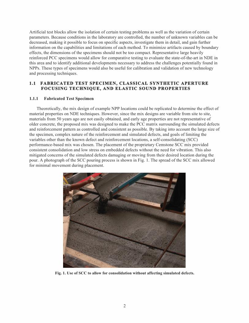
Theoretically, the mix design of example NPP locations could be replicated to determine the effect of material properties on NDE techniques. However, since the mix designs are variable from site to site, materials from 50 years ago are not easily obtained, and early age properties are not representative of older concrete, the proposed mix was designed to make the PCC matrix surrounding the simulated defects and reinforcement pattern as controlled and consistent as possible. By taking into account the large size of the specimen, complex nature of the reinforcement and simulated defects, and goals of limiting the variables other than the known defect and reinforcement locations, a self-consolidating (SCC) performance-based mix was chosen. The placement of the proprietary Cemstone SCC mix provided consistent consolidation and low stress on embedded defects without the need for vibration. This also mitigated concerns of the simulated defects damaging or moving from their desired location during the pour. A photograph of the SCC pouring process is shown in Fig. 1. The spread of the SCC mix allowed for minimal movement during placement.

Fig. 1. Use of SCC to allow for consolidation without affecting simulated defects.

3

The simulated defects were embedded to determine how the current state-of-the-practice NDE techniques will be able to determine various forms of degradation in NPP concrete structures. This is a difficult task since, to date, limited comparisons of state-of-the-art methods have been conducted at the size and reinforcement density of LWR containment structures on controlled specimens, or verified through forensic activities. The constructed specimen is designed to allow for assessment of controlled benchmark defects from previous studies in a more heavily reinforced concrete structure as well as evaluation of realistic defects to ensure that the correct type of features for effective NPP NDE are included.

1.1.2 Classical Synthetic Aperture Focusing Technique

As documented in ONRL/TM-2013/430, ultrasonic linear array devices with 40 or more transducers performed best at volumetric imaging [8]. These devices are based on the “pitch-catch” method of sending and receiving shear wave impulses at the surface, requiring only one-sided access and receiving the echoes at the original surface. Fig. illustrates how the “pitch-catch” method examines the volume under the instrument.

Fig. 2. Pitch-Catch method illustrated.

Improvements in transducer coupling technology have increased productivity by eliminating the need for application of a coupling agent to transfer the vibration to the concrete. The transducers have been developed to transmit and receive shear wave impulses, which allows for measurement pairs with multiple angles of transmission and reception at reduced transducer spacing for high-precision shear wave impulse measurements, and eliminates the need for a manual mechanical impact. The redundancy and spatial diversity of the measurements provide an opportunity to use the Kirchoff migration-based focusing

4

technique to create cross sections of the subsurface structure that correlate to the physical location of the internal concrete structure.

The additional thickness of concrete in NPP applications drastically decreases the signal-to-noise ratio on returned ultrasound signals since the signals must travel through the concrete twice so the echo can be received and analyzed. Even though previous results for thinner structures show promise in the ability to nondestructively evaluate internal characteristics, the results need to be validated for thicker and more heavily reinforced structures. There are two major NDE challenges associated with the fabrication and evaluation of thicker structures:

• Low signal-to-noise ratio with greater depths due to heterogeneous material such as PCC with a dense and complex arrangement of reinforcements.

• Effects from vertical boundaries at similar distances to the region of interest (ROI).

1.1.3 Elastic Sound Properties

A background on elastic wave propagation, which is the basis of the linear array ultrasonic technique used for the data collection in this study, allows for a discussion of these challenges. When exposed to a short duration external impact, the concrete reacts approximately like an elastic solid medium, where the distortion and subsequent movements in the concrete can be described using three general modes of wave propagation categorized by the coverage and direction of particle motion with respect to propagation direction: p-waves, s-waves, and r-waves.

The compression (also known as longitudinal or primary) waves (p-waves) have particle motion parallel with the direction of wave propagation. The four transverse (also known as shear) waves (s waves) have particle motion perpendicular to the wave propagation direction. The Rayleigh waves (r waves) have retrograde elliptical particle motion. The r-waves propagate along the surface, whereas the p- and s-waves propagate throughout the body of the solid in a hyperbolic nature [9]. The reflection of p- and s-waves depends on changes in acoustic impedance from internal characteristics of concrete structures. P- and s-waves are useful in evaluating internal characteristics of concrete structures with only one-sided access because changes in subsurface properties such as flaws, inclusions, or layer boundaries cause reflections back to the surface.

A few observations can be made from these relationships with regard to use of elastic waves for evaluation of thick reinforced concrete structures. Since acoustic impedance is positively correlated to the stiffness of the material, elastic waves are extremely proficient at characterizing interfaces such as cracks, voids, or delamination where the change in acoustic impedance from concrete to air is extremely high. However, since PCC is composed of air voids and aggregates, elastic waves can also experience significant attenuation that limits the penetration depth. For example, since the p-wave has the lowest amount of energy from a point source impact, it may not achieve the necessary penetration depth required to characterize the thick concrete specimen due to the low energy content. However, the ability to propagate in all types of media may provide air-coupled possibilities [10]. S-waves have significantly higher energy content, allowing for greater penetration depth in heterogeneous media such as concrete. However, they require a solid material for propagation, creating a need for ground coupling. Moreover, because they are similar in velocity to r-waves, boundary effect interference may be a problem.

Unlike the loss of signal-to-noise ratio with greater penetration depth problem, which needs to be addressed solely by the NDE technique, the boundary effect problem is less of an issue for in-service inspection of commercial NPP containment structures, where lateral boundaries are less prevalent. However, boundary effects are more critical for thicker concrete structures with regards to specimen design. For many NDE techniques, the first reflected wave received is assumed to be from internal changes in acoustic impedance, or the rear surface, assuming the structure is infinitely expanded in the lateral direction. This assumption is generally valid for evaluation of continuous structures such as NPP containment walls and for internal interrogation of specimens of thin structures such as bridge decks or pavements. However, to use this assumption and properly represent NPP containment structures, thicker concrete structure specimens require higher restrictions for allowable vertical boundaries.

5

11.2 WAVELET DECOMPOSITION

The Time Frequency (TF) technique forming the core of our approach is the wavelet packet decomposition. However, instead of directly using the coefficients from the wavelet packet decomposition, we decompose the original received ultrasound signals into various frequency bands (nodes), select a node based on the frequency band it contains, and then reconstruct the node back to a time-series dataset with the same duration and sampling rate as the original signal. However, this reconstructed dataset contains only the specific band of frequencies contained in the reconstructed node. This process takes advantage of the reconstruction property of the mother wavelet, and the natural frequency segmentation provided by the continued decomposition of the previous decomposition results’ nodes. Any decomposition node can be reconstructed. The end effect is a highly selective analysis of the received signal’s frequency content, which can be visualized using the familiar and reliable SAFT image reconstruction algorithm.

1.2.1 Wavelets

Far more in-depth and detailed introductions to wavelets and multi-resolution analysis can be found in numerous publications such as [11], [12], and [13]. The basics are described below.

The mother wavelet, also known as a basis function, is scaled and translated and then “compared” (i.e., convolved) with the signal being analyzed as shown in Eq. (1), where a is the scale factor, τ is the translation parameter, t is time, x is the signal, and ψ is the mother wavelet [11]

. Equation 1

Using the multi-resolution analysis approach, each scaling and translation of the mother wavelet is

convolved with the signal being analyzed, resulting in a decomposition of the analyzed signal into two nodes. These two decomposition nodes each contain half the bandwidth of the signal that was decomposed. The node containing the lower half of the original bandwidth is called the approximation. The node containing the upper half of the bandwidth is called the detail. Detail nodes and approximation nodes can be further decomposed. The results of an individual node’s decomposition create two more nodes. One node contains the upper half of the decomposed node’s bandwidth, while the other contains the lower half of the decomposed node’s bandwidth. A graphical representation of this is shown in Fig. 3.

When the scale and translation parameters are swept across a continuous range, this convolution is known as the Continuous Wavelet Transform (CWT). Similarly, the Discrete Wavelet Transform (DWT) is the “adjustment” of the scale and translation parameters in discrete steps [13]. We perform a selective CWT packet decomposition.

1.2.2 Wavelet Packet Decomposition

The motivation behind the use of wavelet packet decomposition over wavelet decomposition is based on the greater level of selectivity provided by wavelet packet decomposition. When performing a wavelet decomposition, only the approximation portion is decomposed by each successive decomposition as shown in Fig. 3(a). For wavelet packet decompositions, any approximation or detail can be decomposed, which Daubechies terms as the “splitting trick [13],” and is illustrated in Fig. 3(b). This allows a greater range of frequency bands and bandwidths to be selected and analyzed. Wavelet packet decomposition has the same advantageous properties as wavelet decomposition. The most important properties to this application are the low-frequency leakage and exact reconstruction properties.

dtttxaCWT a )()(),( ττ Ψ= ∫

6

(a)

(b)

Fig. 3. (a) Block diagram of wavelet decomposition and (b) block diagram of a wavelet packet decomposition.

The sampling rate of the commercial ultrasonic inspection system used in the collection of the analyzed data is 1 MHz. Based on Nyquist criteria the collected data contains 500 kHz of bandwidth. This allows for an alias free spectral content of 0 Hz (DC) through 500 kHz. The frequency banding method [14] used is based on wavelet packet decomposition. Ultimately, the end effect is that the bandwidth (spectral content) of a decomposed node is divided between the two resulting nodes. As an illustration, Node 0 is the starting point of the decomposition. It contains all 500 kHz of bandwidth. Node 0 is then decomposed into two new nodes, Node 1 and Node 2. Node 1 contains the lower half of the bandwidth, 0 Hz through 250 kHz. Likewise, Node 2 contains the upper half, 250 kHz through 500 kHz. There is a small amount of frequency leakage between the two new nodes at the dividing point, 250 kHz. At this point, the decomposition continues following the same principle. The bandwidth (spectral content) of Node 1 is split to form Nodes 3 and 4. Node 2 is split to form Nodes 5 and 6. In all cases, each child node contains half of the bandwidth (spectral content) of its parent.

7

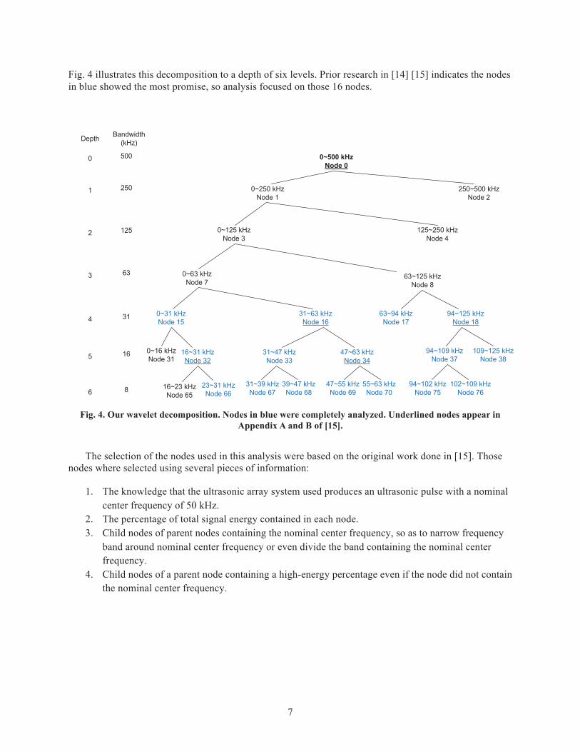
Fig. 4 illustrates this decomposition to a depth of six levels. Prior research in [14] [15] indicates the nodes in blue showed the most promise, so analysis focused on those 16 nodes.

Depth

0~500 kHzNode 0

0~250 kHzNode 1

250~500 kHzNode 2

0

1

0~125 kHzNode 3

125~250 kHzNode 4

2

0~63 kHzNode 7

3

4

5

63~125 kHzNode 8

0~31 kHzNode 15

31~63 kHzNode 16

63~94 kHzNode 17

94~125 kHzNode 18

0~16 kHzNode 31

16~31 kHzNode 32

31~47 kHzNode 33

47~63 kHzNode 34

94~109 kHzNode 37

109~125 kHzNode 38

616~23 kHzNode 65

23~31 kHzNode 66

31~39 kHzNode 67

39~47 kHzNode 68

47~55 kHzNode 69

55~63 kHzNode 70

94~102 kHzNode 75

102~109 kHzNode 76

Bandwidth(kHz)

500

250

125

63

31

16

8

Fig. 4. Our wavelet decomposition. Nodes in blue were completely analyzed. Underlined nodes appear in Appendix A and B of [15].

The selection of the nodes used in this analysis were based on the original work done in [15]. Those

nodes where selected using several pieces of information:

1. The knowledge that the ultrasonic array system used produces an ultrasonic pulse with a nominal center frequency of 50 kHz.

2. The percentage of total signal energy contained in each node. 3. Child nodes of parent nodes containing the nominal center frequency, so as to narrow frequency

band around nominal center frequency or even divide the band containing the nominal center frequency.

4. Child nodes of a parent node containing a high-energy percentage even if the node did not contain the nominal center frequency.

8

9

22. RECONSTRUCTION OF ASR AND FREEZE THAW SPECIMENS

2.1 WAVELET PACKET DECOMPOSITION RECONSTRUCTION OF ASR AND NON-ASR SPECIMENS

This Section compares the results of the wavelet packet decomposition technique Node zero, the original reconstruction, with reconstruction from other nodes to ascertain if wavelet filtering of the datasets increases the contrast between and/or discrimination of non-ASR from ASR samples.

With the goal of increased discrimination of ASR from non-ASR samples, various wavelet filter banks were implemented on the raw US datasets before SAFT reconstruction to investigate their impact

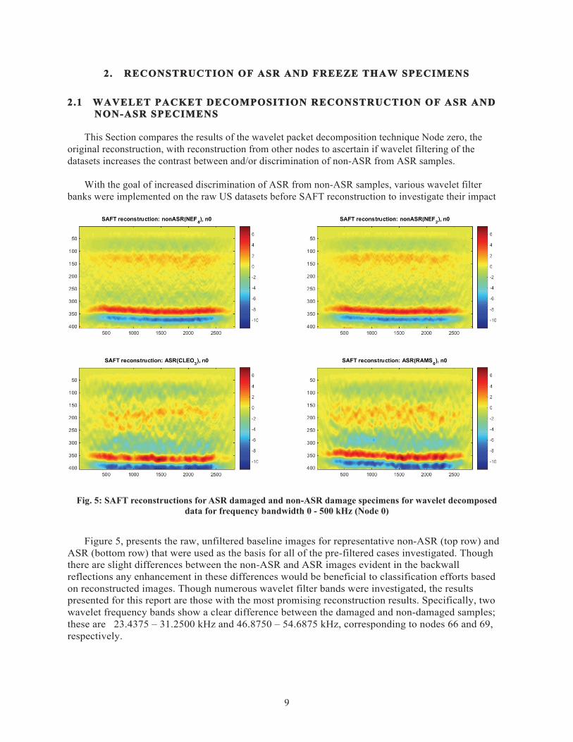
Fig. 5: SAFT reconstructions for ASR damaged and non-ASR damage specimens for wavelet decomposed data for frequency bandwidth 0 - 500 kHz (Node 0)

Figure 5, presents the raw, unfiltered baseline images for representative non-ASR (top row) and

ASR (bottom row) that were used as the basis for all of the pre-filtered cases investigated. Though there are slight differences between the non-ASR and ASR images evident in the backwall reflections any enhancement in these differences would be beneficial to classification efforts based on reconstructed images. Though numerous wavelet filter bands were investigated, the results presented for this report are those with the most promising reconstruction results. Specifically, two wavelet frequency bands show a clear difference between the damaged and non-damaged samples; these are 23.4375 – 31.2500 kHz and 46.8750 – 54.6875 kHz, corresponding to nodes 66 and 69, respectively.

10

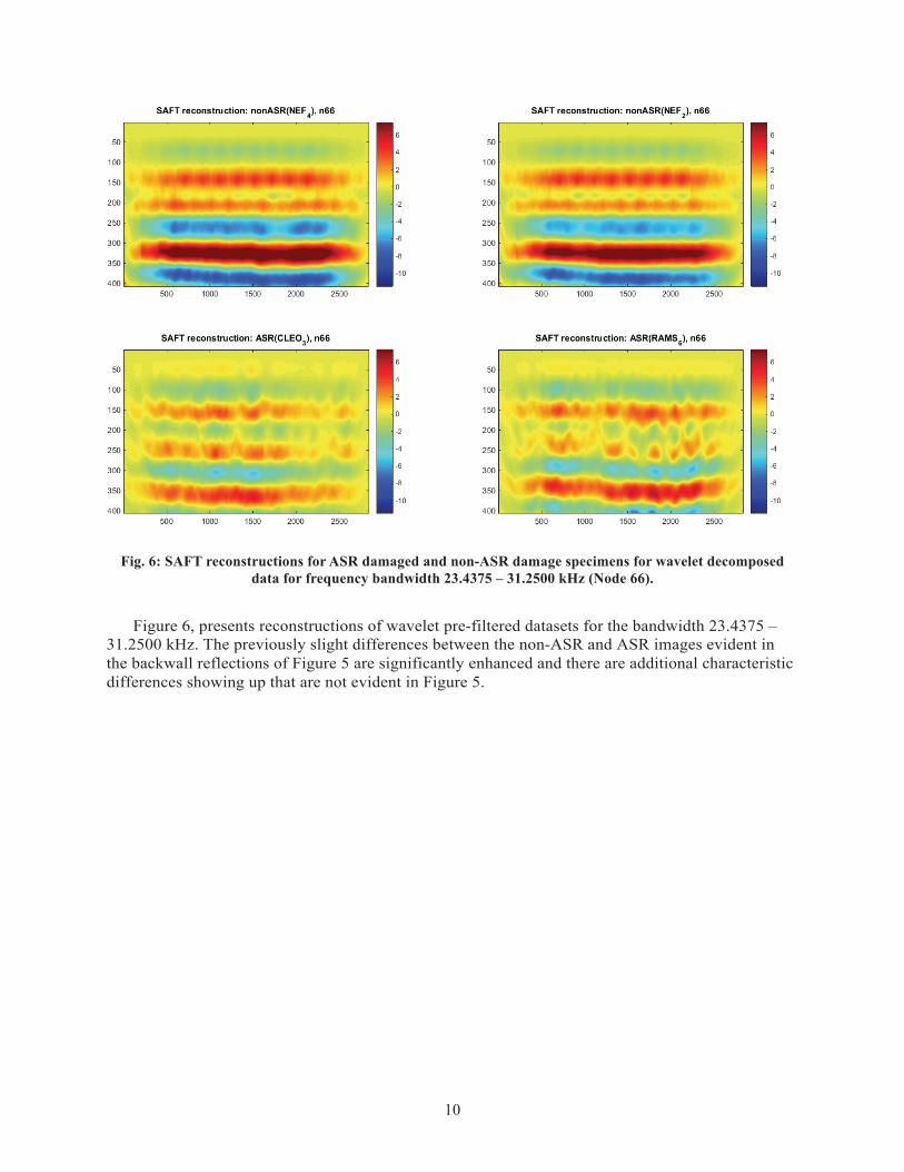
Fig. 6: SAFT reconstructions for ASR damaged and non-ASR damage specimens for wavelet decomposed data for frequency bandwidth 23.4375 – 31.2500 kHz (Node 66).

Figure 6, presents reconstructions of wavelet pre-filtered datasets for the bandwidth 23.4375 –

31.2500 kHz. The previously slight differences between the non-ASR and ASR images evident in the backwall reflections of Figure 5 are significantly enhanced and there are additional characteristic differences showing up that are not evident in Figure 5.

11

Fig. 7: SAFT reconstructions for ASR damaged and non-ASR damage specimens for wavelet decomposed data for frequency bandwidth 46.8750 – 54.6875 kHz (Node 69)

Figure 7, presents reconstructions of wavelet pre-filtered datasets for the bandwidth 46.8750 –

54.6875 kHz. Again different characteristics of the differences between the non-ASR and ASR images are highlighted in the backwall reflections as compared to those of Figures 5 and 6.

Though there are clear visible differences in the results presented in Figures 5-7, we are still

investigating a suitable image quality metric that robustly quantitates this. For an example, we are currently investigating the use of entropy or structural similarity index (SSI) to capture the differences seen in the images in terms of image signal content. Though we have investigated various ASR sample population normalization strategies in conjunction with this effort, as of the time of this report, we have not yet arrived at a robust implementation of either of the aforementioned options.

12

13

33. MODEL-BASED ITERATIVE RECONSTRUCTION

3.1 OVERVIEW

As described above, NDE of complex, non-homogenous, thick objects may extend the operational life of nuclear facilities, bridges, and production wells and provide better characterization of hard to access sub-surfaces. Unlike homogeneous materials, such as many metals, reinforced concrete used in NPPs is a heterogeneous material, a composite with a low-density matrix, a mixture of cement, sand, aggregate and water, and a high-density reinforcement, made up of steel rebar or tendons. This structural complexity makes NDE a challenging task. The state-of-the-art technology that is currently used to evaluate these structures is called Synthetic Aperture Focusing Technique (SAFT) [16, 17, 18]. While acoustic imaging using the SAFT works adequately well for thin specimens of concrete or for steel inspection, enhancements are needed for heavily reinforced, thick concrete.

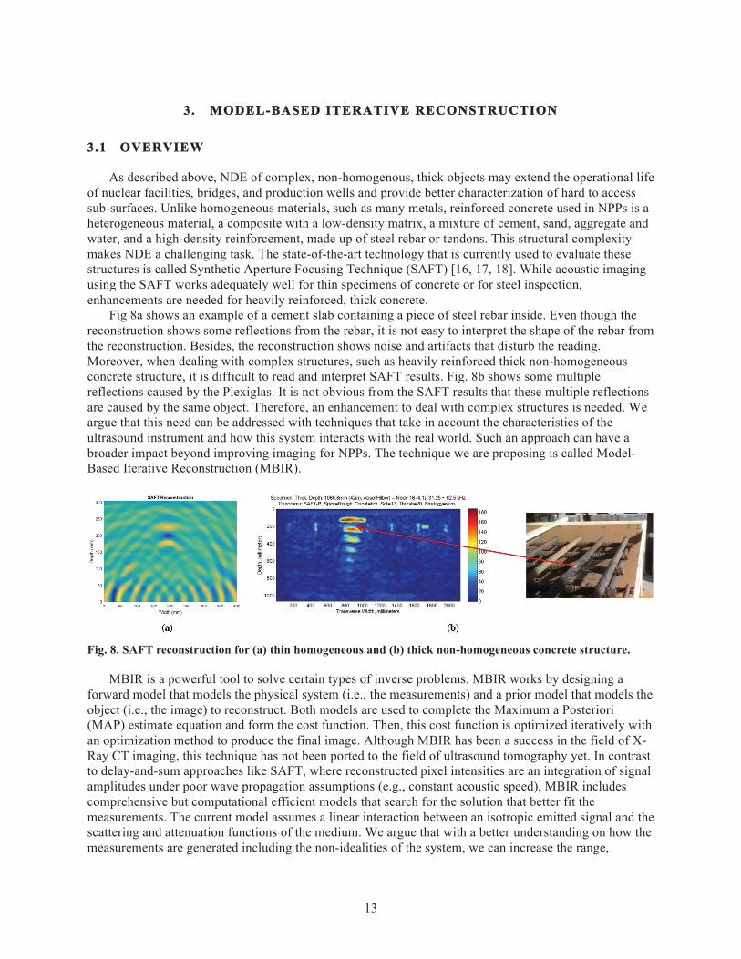
Fig 8a shows an example of a cement slab containing a piece of steel rebar inside. Even though the reconstruction shows some reflections from the rebar, it is not easy to interpret the shape of the rebar from the reconstruction. Besides, the reconstruction shows noise and artifacts that disturb the reading. Moreover, when dealing with complex structures, such as heavily reinforced thick non-homogeneous concrete structure, it is difficult to read and interpret SAFT results. Fig. 8b shows some multiple reflections caused by the Plexiglas. It is not obvious from the SAFT results that these multiple reflections are caused by the same object. Therefore, an enhancement to deal with complex structures is needed. We argue that this need can be addressed with techniques that take in account the characteristics of the ultrasound instrument and how this system interacts with the real world. Such an approach can have a broader impact beyond improving imaging for NPPs. The technique we are proposing is called Model-Based Iterative Reconstruction (MBIR).

Fig. 8. SAFT reconstruction for (a) thin homogeneous and (b) thick non-homogeneous concrete structure.

MBIR is a powerful tool to solve certain types of inverse problems. MBIR works by designing a forward model that models the physical system (i.e., the measurements) and a prior model that models the object (i.e., the image) to reconstruct. Both models are used to complete the Maximum a Posteriori (MAP) estimate equation and form the cost function. Then, this cost function is optimized iteratively with an optimization method to produce the final image. Although MBIR has been a success in the field of X-Ray CT imaging, this technique has not been ported to the field of ultrasound tomography yet. In contrast to delay-and-sum approaches like SAFT, where reconstructed pixel intensities are an integration of signal amplitudes under poor wave propagation assumptions (e.g., constant acoustic speed), MBIR includes comprehensive but computational efficient models that search for the solution that better fit the measurements. The current model assumes a linear interaction between an isotropic emitted signal and the scattering and attenuation functions of the medium. We argue that with a better understanding on how the measurements are generated including the non-idealities of the system, we can increase the range,

14

resolution, and image quality of the ultrasound system; with the end-goal of producing quantitative measurements of the physical properties of the medium under interrogation.

33.2 MODEL-BASED ITERATIVE RECONSTRUCTION

Model-Based Iterative Reconstruction (MBIR) is an image reconstruction framework that embraces the integrated imaging philosophy, where the hardware and software are tailored to provide the most informative measurements. It is a powerful probabilistic tool that has been proven to be very effective for reconstruction in many applications, such as X-ray Computed Tomography (CT) [19], Positron Emission Tomography (PET) [20], and electron tomography [21]. In particular, the method has been extensively applied to the reconstruction of X-ray Computed Tomography (CT) with an image quality superior to that of state-of-the-art filter back projection techniques. MBIR shows equivalent image quality even after X-ray dose reductions of up to 80% [22, 23]. This reduction in X-ray dose is a testament to the robustness of the system in the presence of noise and sparse information collection, which are usually the interrogation conditions for thick concrete.

A typical MBIR problem contains two main parts: the forward model that models the physical system (i.e., the measurements), and the prior model that models the object (i.e., the object image) to be reconstructed. When these models are combined, they form the cost function. Optimizing the cost function will produce the solution to the Maximum a Posteriori (MAP) estimate, given by

Equation 2

where is the cost function [24]. For every iteration and based on the current object image estimate, the MBIR model produces synthetic measurements that are compared against the real data. Then, the difference (e.g., the error) is used to update the object estimate for the next iteration. Fig. 9 shows a flowchart of a typical MBIR algorithm. The models in MBIR are important to understand the probabilistic behavior of the error and to regularize the reconstruction at each iteration. In order to obtain good results and better resolution and contrast for certain applications, the forward and prior models might need to be more complex or non-linear. This in return will make optimizing the cost function very computationally expensive. Therefore, the real challenge in ultrasound MBIR is to find a way to lower the computational cost while preserving the complexity of the models. Many optimization methods, such as Iterative Coordinate Descent (ICD), have been introduced to overcome this issue. Also, several methods have been proposed to approximate complex or non-linear model, such as Taylor Approximation, to lower the computational cost.

15

Fig. 9. Flowchart of a typical MBIR reconstruction algorithm.

There are alternate iterative reconstruction methods, such as iterative Maximum Likelihood Estimation (MLE) [25], and Simultaneous Iterative Reconstruction Technique (SIRT) [26]. The main difference between MBIR and MLE is that MLE does not require a prior model of the object, which can be sensitive to random variation in data. The prior model is necessary to regulate the estimation and reduce variance. However, this will require having an accurate prior model. Similarly, SIRT does not require a prior model, either, and does not require a probabilistic model for the measurements [27]. In addition, there are a few iterative non-MBIR reconstruction methods for ultrasound, such as the Born Iterative Method (BIM), which is combined with Total Variation (TV) minimization for Ultrasound Computed Tomography (UCT) using compressed sensing (CS) [28], and the Iterative Inverse Non-Uniform Fast Fourier Transform (NUFFT), which is used in diffraction UCT [29]. While these methods can produce excellent results, they are intended for transmission measurements. In this paper, we show an MBIR implementation for one-sided ultrasound applications.

3.2.1 Ultrasonic MBIR

To apply MBIR to the ultrasonic signals, we need to formulate the forward model, , and the prior model, , where is the observed data and is the unknown Intensity Reflectivity Coefficients (IRC). The forward model, , is obtained from the equation

Equation 3

where A is the system matrix, W is a Gaussian random vector with distribution , and is a diagonal matrix with statistical weights. From Eq. 3, is a Gaussian random vector with distribution

which allows to express the forward statistical model as

Equation 4

16

In order to compute the system matrix A, we will consider an ultrasound system that probes a position in a homogeneous medium [30] by transmitting a signal from the ith transducer located at position and receives the reflected signal at the jth transducer located at position . If the medium is

linear, homogeneous, and isotropic, then the transfer function from the transmitter to the point p is given by

Equation 5

where

Equation 6

is the rate of attenuation in , and

Equation 7

is the phase delay due to propagation through the medium [29]. Similarly, the transfer function from the point p to the receiver is given by

. Equation 8

Let be the transmitted signal, and let be the IRC of the voxel at location p that we would like to estimate. Then, the received signal due to reflections from the voxel at location p is given by

Equation 9

where is the Fourier transform of , and

Equation 10

From Eq. 9, the system Point Spread Function (PSF) is defined as

Equation 11

Then, the received signal amplitude at time t is given by

. Equation 12

Finally, the full signal transmitted and received by transducer i and j, respectively is computed by integrating over p.

Equation 13

.

.

17

where the system matrix is defined as

Equation 14

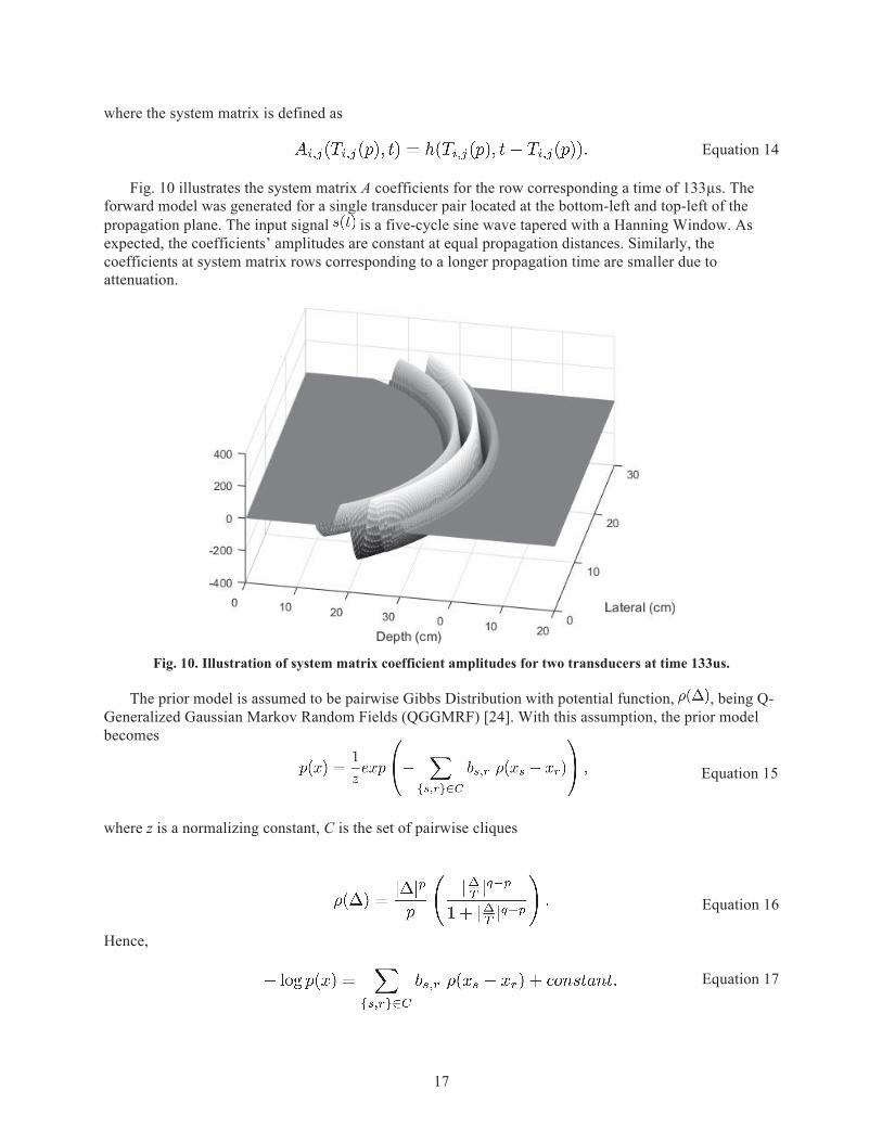
Fig. 10 illustrates the system matrix A coefficients for the row corresponding a time of 133µs. The forward model was generated for a single transducer pair located at the bottom-left and top-left of the propagation plane. The input signal is a five-cycle sine wave tapered with a Hanning Window. As expected, the coefficients’ amplitudes are constant at equal propagation distances. Similarly, the coefficients at system matrix rows corresponding to a longer propagation time are smaller due to attenuation.

Fig. 10. Illustration of system matrix coefficient amplitudes for two transducers at time 133us.

The prior model is assumed to be pairwise Gibbs Distribution with potential function, , being Q-Generalized Gaussian Markov Random Fields (QGGMRF) [24]. With this assumption, the prior model becomes

Equation 15

where z is a normalizing constant, C is the set of pairwise cliques

Equation 16

Hence,

Equation 17

18

The pairwise Gibbs distribution was chosen, because it models natural existing edges more accurately. QGGMRF was chosen because it guarantees function convexity, models sharp discontinuities, and tends to generate fewer reconstruction artifacts.

After formulating the forward and prior models, the MAP estimate is complete, i.e.

Equation 18

Equation 19

Equation 20

Eq. 19 is optimized using Iterative Coordinate Descent algorithm (ICD). For this kind of MAP estimate or cost function, ICD is stable, fast, and efficient and tends to emphasize high frequency components on low contrast regions. Fig. 11 shows a general ICD algorithm to solve such cost functions.

Fig. 11. ICD Algorithm.

3.2.2 Forward Model Crosstalk Upgrade

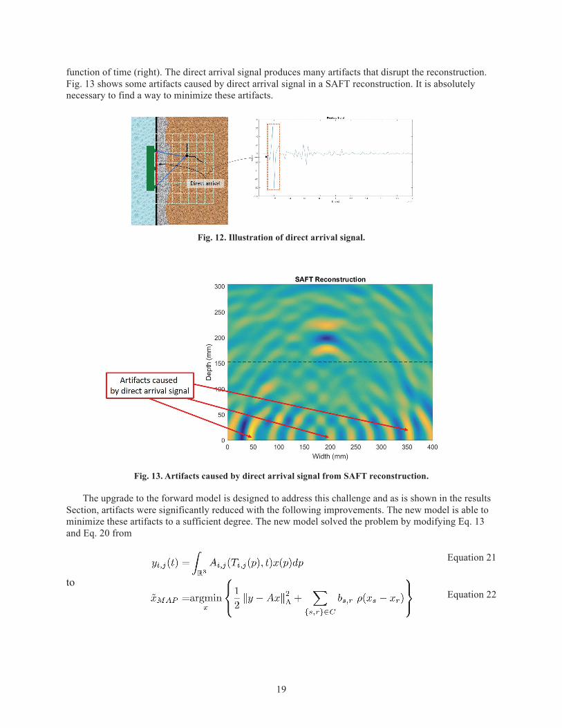
The forward model in the previous section does not account for the direct arrival signal or crosstalk. The direct arrival signal is a surface wave signal that is received directly from transmitter to receiver. Fig. 12 shows an example of direct arrival signal in the field of view (left) and in the measurements as a

19

function of time (right). The direct arrival signal produces many artifacts that disrupt the reconstruction. Fig. 13 shows some artifacts caused by direct arrival signal in a SAFT reconstruction. It is absolutely necessary to find a way to minimize these artifacts.

Fig. 12. Illustration of direct arrival signal.

Fig. 13. Artifacts caused by direct arrival signal from SAFT reconstruction.

The upgrade to the forward model is designed to address this challenge and as is shown in the results Section, artifacts were significantly reduced with the following improvements. The new model is able to minimize these artifacts to a sufficient degree. The new model solved the problem by modifying Eq. 13 and Eq. 20 from

Equation 21

to Equation 22

20

where rj is the position of the receiver, zi,j is a scaling coefficient, d is the discretized version of , z is a vector containing all the zi,j coefficients for each measurement. The solution for

the MAP estimate of z is

Equation 23

Equation 24

Equation 25

Eq. 24 is easy to compute because (dtd) is a diagonal matrix, defined as

Equation 26

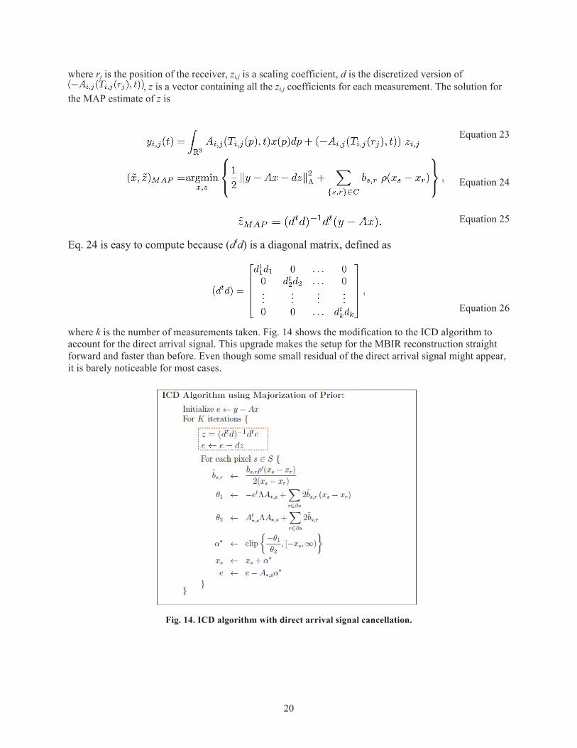
where k is the number of measurements taken. Fig. 14 shows the modification to the ICD algorithm to account for the direct arrival signal. This upgrade makes the setup for the MBIR reconstruction straight forward and faster than before. Even though some small residual of the direct arrival signal might appear, it is barely noticeable for most cases.

Fig. 14. ICD algorithm with direct arrival signal cancellation.

j

21

33.3 SIMULATED AND EXPERIMENTAL RESULTS

Simulated data for an ultrasonic phased array system has been obtained using a third party simulator called K-Wave [30]. All simulated tests are assumed to be for a homogeneous cement slab with acoustic speed of 3,680 m/s and attenuation coefficient of 1.5 × 10−6 . The ultrasound system is defined as non-focused isotropic sources and sensors, where the input signal is a 3-cycle sine wave with a central frequency of 52KHz. Four test samples were generated for a medium size of 40 cm wide and 30 cm deep. In addition, 10 equally spaced transducers are used as transmitters and receivers. Each sample has a different phantom test: thin steel plate, thick steel plate, long and short thin steel plates, and point scatters. Fig. 15 illustrates the position of the transducer with respect the specimen.

Fig. 15. Illustration of ultrasound system position relative to specimens.

Usually, the MBIR algorithm is initialized with a low frequency (i.e., blurred) version of the object. The low frequency initial object estimate could be obtained from a back projection x0 = AT y or from other reconstruction techniques such as SAFT. Since the cost function is strictly convex, any initialization will lead to the same answer. For the experiments below, the MBIR algorithm is initialized with a zero initialization for simplicity and unbiased convergence. The simulated data is used to get reconstruction results from both SAFT and MBIR. The results will be analyzed to compare both reconstruction techniques. However, the results will also be used to show some challenges to the current MBIR models. Currently, the SAFT model and MBIR forward model share the same acoustic assumptions—the specimen is homogeneous, sources are isotropic, and the models are linear. These are acceptable assumptions for simple structures. The results will show that for complex structures, these assumptions do not hold. One of the powerful features of MBIR is that its forward and prior model can always be enhanced to match real physical behavior.

Fig. 16 to Fig. 19 shows all the results obtained from simulated data. The transducers are placed at the bottom or at the left of the 2D reconstructions and 3D surface plots, respectively. The 3D images are obtained from the Matlab ’mesh’ function of the SAFT and MBIR cross-section 2D reconstructions. First, test sample in Fig. 16 is the sample for a thin steel plate. The steel plate appears in both methods. However, SAFT produces a more artifacts caused by the direct arrival signals. Also, noise appears everywhere in the image, and the shape of the object is not well defined. On the other hand, the reconstruction from MBIR is cleaner and clearer, most of the artifacts and noise are removed, and the

22

shape of the object is well defined and easy to interpret. Second, the test sample in Fig. 17 is the sample for the thick steel plate. The analysis is similar to the test sample in Fig. 16. However, in both SAFT and MBIR, the steel plate appears to be thinner than it should. This happened because it was assumed by both methods that the medium is homogeneous and has constant speed. Since sound travels faster in steel than in cement, both methods produced a thinner plate. Therefore, to image thick or large objects, modeling of a non-homogeneous medium is needed. Third, the test sample in Fig. 18 is the sample for long and short thin steel plates. This test was performed to assess the performance of the reconstruction technique when back features (e.g., short plate) are occluded by front features (e.g., long plate). The results are similar to the test sample in Fig. 16. However, the short plate is highly attenuated in both SAFT and MBIR. This is because both methods assume linearity. The reflection from the short plate is further attenuated by the long plate because of non-linearity. This is an example where a nonlinear model is required to image such structures. Next, the test sample in Fig. 19 is the sample for point scatters. This test was performed to analyze the reconstruction from weak reflections. Five point scatters were placed, and they all appeared in the SAFT and MBIR reconstruction. However, MBIR produced some artifacts at the bottom similar to the ones in SAFT. The reason this happened is because the residual of the direct arrival signal cancellation performed by MBIR is greater than the reflected signal from the point scatters. Therefore, MBIR considers the artifacts as information and allows it to pass. Even though MBIR produced artifacts for this test, it can be shown that the SNR is reduced for the SAFT reconstruction.

Fig. 16. Comparison between SAFT and MBIR from simulated data of a thin steel plate: (a) Ground Truth, (b) SAFT Reconstruction, (c) MBIR Reconstruction, (d) SAFT Surface Plot, and (e) MBIR Surface Plot.

Fig. 17. Comparison between SAFT and MBIR from simulated data of a thick steel plate: (a) Ground Truth, (b) SAFT Reconstruction, (c) MBIR Reconstruction, (d) SAFT Surface Plot, and (e) MBIR Surface Plot.

23

Fig. 18. Comparison between SAFT and MBIR from simulated data of a thin long and short steel plates: (a) Ground Truth, (b) SAFT Reconstruction, (c) MBIR Reconstruction, (d) SAFT Surface Plot, and (e) MBIR

Surface Plot.

Fig. 19. Comparison between SAFT and MBIR from simulated data of a steel point scatters: (a) Ground Truth, (b) SAFT Reconstruction, (c) MBIR Reconstruction, (d) SAFT Surface Plot, and (e) MBIR Surface

Plot.

Experimental data has been obtained from a cement slab with a steel rebar placed in the center. Fig. 20 shows the experiment performed. The estimated acoustic speed for the cement is 2,500 m/s, the input signal has a central frequency of 52 kHz, and the medium size is 40cm wide and 30cm deep. Fig. 21 shows the SAFT and MBIR reconstruction results from this real dataset. The analysis of the results is similar to the analysis of the test sample in Fig. 16. Moreover, this experimental data comparison is the most important reconstruction due to the fact that this real data reconstruction supports our claim that better reconstruction can be obtained if the reconstruction technique’s assumptions better matches those of the real world. In addition, we get this improvement with minimal trade in computational cost. SAFT reconstruction takes less than a second while MBIR reconstructions can be obtained in about 11 seconds.

Fig. 20. Real data obtained from a MIRA system with 40 transducers. The specimen is a cement slab with a steal rebar in the center.

24

Fig. 21. Comparison between SAFT and MBIR from real data for a concrete slab with a rebar at the center: (a) Ground Truth, (b) SAFT Reconstruction, (c) MBIR Reconstruction, (d) SAFT Surface Plot, and (e) MBIR

Surface Plot.

33.4 MBIR CLOSING REMARKS

We demonstrated an MBIR implementation for a one-sided ultrasonic phased array system. This implementation has been enhanced to eliminate the artifacts caused by direct arrival signals. We compared MBIR reconstruction results with SAFT reconstruction results using simulated and experimental data. We showed that MBIR is a much better replacement for SAFT. We also showed some challenges to the current model. One of the powerful features of MBIR is that its forward and prior model can always be enhanced and upgraded to match the physical system and address current limitations and challenges. Our goal is to improve MBIR’s current models to account for more complex structures, such as heavily reinforced thick concrete structures, and model elastic non-linear effects, such as mode conversion and diffraction. Therefore, the future work for this research is to upgrade the forward model from a simple model, which is homogeneous, isotropic, and linear, to a complex model, which should be non-homogeneous, anisotropic, and non-linear. Our biggest challenge is to incorporate these complex features while keeping the forward model tractable and computationally efficient. Also, results from a wide variety of real experiments will be shown for future publication.

25

44. UNIVERSAL NDE DATASET FRAMEWORK

4.1 INTRODUCTION

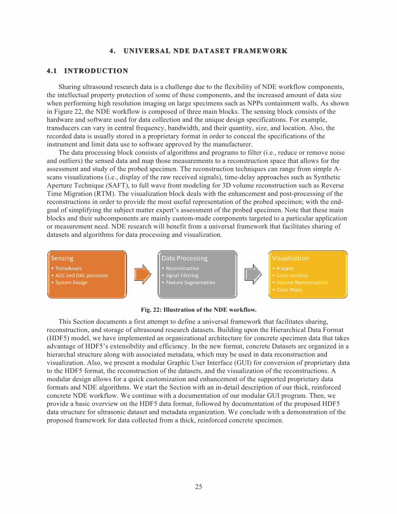
Sharing ultrasound research data is a challenge due to the flexibility of NDE workflow components, the intellectual property protection of some of these components, and the increased amount of data size when performing high resolution imaging on large specimens such as NPPs containment walls. As shown in Figure 22, the NDE workflow is composed of three main blocks. The sensing block consists of the hardware and software used for data collection and the unique design specifications. For example, transducers can vary in central frequency, bandwidth, and their quantity, size, and location. Also, the recorded data is usually stored in a proprietary format in order to conceal the specifications of the instrument and limit data use to software approved by the manufacturer.

The data processing block consists of algorithms and programs to filter (i.e., reduce or remove noise and outliers) the sensed data and map those measurements to a reconstruction space that allows for the assessment and study of the probed specimen. The reconstruction techniques can range from simple A-scans visualizations (i.e., display of the raw received signals), time-delay approaches such as Synthetic Aperture Technique (SAFT), to full wave front modeling for 3D volume reconstruction such as Reverse Time Migration (RTM). The visualization block deals with the enhancement and post-processing of the reconstructions in order to provide the most useful representation of the probed specimen; with the end-goal of simplifying the subject matter expert’s assessment of the probed specimen. Note that these main blocks and their subcomponents are mainly custom-made components targeted to a particular application or measurement need. NDE research will benefit from a universal framework that facilitates sharing of datasets and algorithms for data processing and visualization.

Fig. 22: Illustration of the NDE workflow.

This Section documents a first attempt to define a universal framework that facilitates sharing, reconstruction, and storage of ultrasound research datasets. Building upon the Hierarchical Data Format (HDF5) model, we have implemented an organizational architecture for concrete specimen data that takes advantage of HDF5’s extensibility and efficiency. In the new format, concrete Datasets are organized in a hierarchal structure along with associated metadata, which may be used in data reconstruction and visualization. Also, we present a modular Graphic User Interface (GUI) for conversion of proprietary data to the HDF5 format, the reconstruction of the datasets, and the visualization of the reconstructions. A modular design allows for a quick customization and enhancement of the supported proprietary data formats and NDE algorithms. We start the Section with an in-detail description of our thick, reinforced concrete NDE workflow. We continue with a documentation of our modular GUI program. Then, we provide a basic overview on the HDF5 data format, followed by documentation of the proposed HDF5 data structure for ultrasonic dataset and metadata organization. We conclude with a demonstration of the proposed framework for data collected from a thick, reinforced concrete specimen.

26

44.2 THICK, REINFORCED CONCRETE NDE WORKFLOW

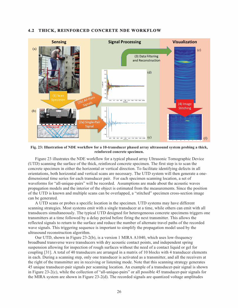
Fig. 23: Illustration of NDE workflow for a 10-transducer phased array ultrasound system probing a thick, reinforced concrete specimen.

Figure 23 illustrates the NDE workflow for a typical phased array Ultrasonic Tomographic Device (UTD) scanning the surface of the thick, reinforced concrete specimen. The first step is to scan the concrete specimen in either the horizontal or vertical direction. To facilitate identifying defects in all orientations, both horizontal and vertical scans are necessary. The UTD system will then generate a one-dimensional time series for each transducer pair. For each specimen scanning location, a set of waveforms for “all-unique-pairs” will be recorded. Assumptions are made about the acoustic waves propagation models and the interior of the object is estimated from the measurements. Since the position of the UTD is known and multiple scans can be overlapped, a “stitched” specimen cross-section image can be generated.

A UTD scans or probes a specific location in the specimen. UTD systems may have different scanning strategies. Most systems emit with a single transducer at a time, while others can emit with all transducers simultaneously. The typical UTD designed for heterogeneous concrete specimens triggers one transmitters at a time followed by a delay period before firing the next transmitter. This allows the reflected signals to return to the surface and reduce the number of alternate travel paths of the recorded wave signals. This triggering sequence is important to simplify the propagation model used by the ultrasound reconstruction algorithm.

Our UTD, shown in Figure 23-2(b), is a version 1 MIRA A1040, which uses low-frequency broadband transverse wave transducers with dry acoustic contact points, and independent spring suspension allowing for inspection of rough surfaces without the need of a contact liquid or gel for coupling [31]. A total of 40 transducers are arranged in a matrix of 10 blocks with 4 transducer elements in each. During a scanning step, only one transducer is activated as a transmitter, and all the receivers at the right of the transmitter are in receiving or listening mode. Note that this scanning strategy generates 45 unique transducer-pair signals per scanning location. An example of a transducer-pair signal is shown in Figure 23-2(c), while the collection of “all-unique-pairs” or all possible 45 transducer-pair signals for the MIRA system are shown in Figure 23-2(d). The recorded signals are quantized voltage amplitudes

27

that are proportional to the pressure sensed from the mechanical ultrasonic waves. These recorded amplitudes are usually stored in a proprietary file format. Some UTD system includes the signal processing and visualization blocks in a single package. However, for most systems, the collected data is processed offline where more computational resources are available.

As shown in Figure 23-2(e), a cross-section of the specimen is estimated from the “all-unique-pairs” 1D signals. In order to accomplish this task, some assumptions about the system and the ultrasound propagation have to be defined. For SAFT, it is important to define the acoustic speed of the specimen and the relative location of the transducer-pairs. Each reconstruction technique has unique features. Some trade accuracy for speed, such as SAFT, while others compromise speed in order to provide reconstruction images with pixel intensities that correlate to the acoustic properties of the specimen, such as ultrasound MBIR [6]. For large specimens, such as a thick, reinforced concrete slab, a single UTD scan is not enough to fully evaluate the specimen. Therefore, multiple scans are obtained. Usually, the UTD is moved in the vertical or horizontal line direction (e.g., a linescan) where the border of a scan overlaps with the neighbor scan. As shown in Figure 23-2(f), full-length cross-section images of the specimen can be generated from linescans.

From the description above, it is apparent the complexity of the NDE workflow and the potential for customizable sub-components yields an environment that encourages innovation. Our goal is to develop a Universal NDE Framework, which includes a software architecture model and a file storage format that allows researchers to share ultrasound datasets from different UTDs and specimens.

44.3 SOFTWARE ARCHITECTURE: A “PLUG-AND-PLAY” MODEL

In developing an NDE research application, we have considered the needs of analyzing ultrasonic data collected from a variety of commercial UTDs, most with their own proprietary data formats. By allowing different parties to incorporate their own routines for reading proprietary data into the application, it is possible for those with certain format rights to create datasets that are shareable with others for collaborative research or for the purposes of creating standard testing databases. It is also desirable to allow different parties to incorporate their own algorithms for the reconstruction of converted raw data. This allows for a controlled environment to benchmark new algorithms or recreate research for the experimental validation of others’ published results. Therefore, it is desirable to design and develop a modular application with the means to safely integrate user code for the purposes of reading proprietary data and the integration of algorithmic reconstruction and visualization components.

Fig. 24: Illustration of the "Plug-and-Play" design.

Figure 24 illustrates the “Plug-and-Play” software architecture concept. Each puzzle piece represents an independent piece of code that cannot impact the integrity or maintainability of the software package with its addition or removal. The pieces with the underlined text corresponds to the NDE workflow blocks defined by our framework. All other puzzle pieces are defined by the users. The pieces at the top

28

represent modules that are exclusively defined by the user, while the pieces at the bottom are modules that are part of the software package core code. Note that there are empty connectors. These empty connectors represent the capability of the framework to be enhancement on demand. The design goal is to develop independent code modules where the input and outputs are predefined by the interface modules, but whose existence or absence does not affect the functionality, maintainability, and integrity of the overall software package. Following, the NDE workflow description from the previous Section, we are working on the development of three principal interfaces: the data conversion interface, the signal processing interface, and the visualization interface. The male and female connectors represent communication channels. Note that we allow communication between user-developed modules and the corresponding interfaces, but no user-to-user module communication is permitted. This is desirable to avoid dependence on custom module functionalities that can be removed or upgraded in the future. The software package could include implementation of core modules, such as basic SAFT reconstruction code, HDF5 read/write routines, stitching algorithms, etc. User-defined modules can implement and interface or enhance an existing module, if such module allows it. For example, the SAFT module could be design in such a way that another module could be attached in order to allow for frequency banding SAFT reconstruction.

4.3.1 Data Conversion Interface

To convert to HDF5 in our application, users can integrate their own functions for reading proprietary files through the use of a provided data conversion interface class. The UTD Interface class is contained in the cnde.dev package located with the application code. The user must derive their own class from the UTD interface in the cnde.dev package folder. There are several application aspects that the class developer should take into account. For example, in a typical ultrasonic experiment, data is collected from one or several concrete specimens and stored in multiple proprietary files, either as an individual file per specimen, or scan position, or as one file per sequential collection of scans (e.g. a line of scans across one side of the specimen). File names may be auto-generated based upon the time or order of data collection or some other standard. The filename may not explicitly relate to the actual specimen or location in which data was collected from the numerical data contained in each file may be multidimensional in nature, depending on the collection method.

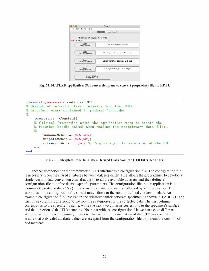
When defining an instance of the UTD interface, the program needs to adapt the class to the unique characteristics of the dataset to convert. On startup, the application automatically locates the user-derived classes in the folder and populates a dropdown menu in the conversion pane of the application. Figure 25 shows a screen shot of the conversion GUI pane. The contents of the dropdown menu pointed to by the red arrow are controlled by the UTD classes that are defined by the user outside of the application. Figure 26 contains boilerplate code for a user-derived class from the UTD interface. The class name is the name used to populate the conversion pane UTD popup menu. The funname and funpath properties must contain the function name and directory path respectively for the user’s function for reading proprietary data files. This removes the need for the user to have a local copy of their code along with the application.

The extension property must contain the proprietary file extension. The application recursively searches for proprietary files from a top-level directory provided by the user. The extension property ensures files of the correct format are located for conversion to HDF5. To convert proprietary files to HDF5 in our application, the user must navigate to the Convert GUI pane, (See Figure 25), of the application and select a UTD from the popup menu. This effectively chooses the appropriate function to read the proprietary data. The user must then select the top-level directory containing all proprietary files of interest and the save directory for the HDF5 file to be created.

29

Fig. 25: MATLAB Application GUI conversion pane to convert proprietary files to HDF5.

Fig. 26: Boilerplate Code for a User-Derived Class from the UTD Interface Class.

Another component of the framework’s UTD interface is a configuration file. The configuration file

is necessary when the shared attributes between datasets differ. This allows the programmer to develop a single, custom data conversion class that apply to all the available datasets, and then define a configuration file to define dataset-specific parameters. The configuration file in our application is a Comma-Separated Value (CSV) file consisting of attribute names followed by attribute values. The attributes in the configuration file should match those in the custom-defined conversion class. An example configuration file, inspired in the reinforced thick concrete specimen, is shown in TABLE 1. The first three columns correspond to the top three categories for the collected data. The first column corresponds to the specimen’s name, while the next two columns correspond to the specimen’s surface and the direction of the UTD scanning. Note that with the configuration file we can assign different attribute values to each scanning direction. The custom implementation of the UTD interface should ensure that only valid attribute values are accepted from the configuration file to prevent the creation of bad metadata.

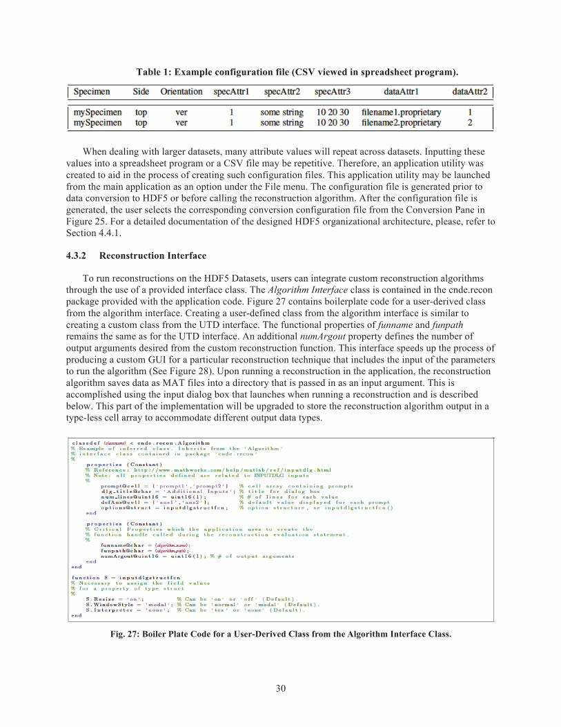
30

Table 1: Example configuration file (CSV viewed in spreadsheet program).

When dealing with larger datasets, many attribute values will repeat across datasets. Inputting these values into a spreadsheet program or a CSV file may be repetitive. Therefore, an application utility was created to aid in the process of creating such configuration files. This application utility may be launched from the main application as an option under the File menu. The configuration file is generated prior to data conversion to HDF5 or before calling the reconstruction algorithm. After the configuration file is generated, the user selects the corresponding conversion configuration file from the Conversion Pane in Figure 25. For a detailed documentation of the designed HDF5 organizational architecture, please, refer to Section 4.4.1.

4.3.2 Reconstruction Interface

To run reconstructions on the HDF5 Datasets, users can integrate custom reconstruction algorithms through the use of a provided interface class. The Algorithm Interface class is contained in the cnde.recon package provided with the application code. Figure 27 contains boilerplate code for a user-derived class from the algorithm interface. Creating a user-defined class from the algorithm interface is similar to creating a custom class from the UTD interface. The functional properties of funname and funpath remains the same as for the UTD interface. An additional numArgout property defines the number of output arguments desired from the custom reconstruction function. This interface speeds up the process of producing a custom GUI for a particular reconstruction technique that includes the input of the parameters to run the algorithm (See Figure 28). Upon running a reconstruction in the application, the reconstruction algorithm saves data as MAT files into a directory that is passed in as an input argument. This is accomplished using the input dialog box that launches when running a reconstruction and is described below. This part of the implementation will be upgraded to store the reconstruction algorithm output in a type-less cell array to accommodate different output data types.

Fig. 27: Boiler Plate Code for a User-Derived Class from the Algorithm Interface Class.

31

Fig. 28: Reconstruction Interface.

The user navigates to the Reconstruction pane, (See Figure 28(a)), in the main GUI, and selects the desired algorithm from a dropdown menu. This action loads the appropriate algorithm for data reconstruction. Then, the user selects the HDF5 file containing the datasets to process. When a reconstruction is requested a GUI with the reconstruction algorithm configuration parameters is shown (See Figure 28(b)). Example inputs could be a save path for created reconstruction files, relaxation parameters in iterative reconstruction approaches, etc. Upon running the reconstruction program, a function handle is created for the user’s custom algorithm and the additional input arguments are passed to an evaluation statement that runs the algorithm. User defined algorithms are assumed to have input arguments following a particular format in order to guarantee correct function with the application. The expected format is as follows:

function ,

where OUTPUT is a vector with the reconstruction algorithm results, data is the dataset to reconstruct, attributesArray is a list of attributes defined in the implementation of the UTD interface for the dataset in data, and the inputsX are the optional reconstruction algorithm configuration parameters entered in the configuration pane similar to the example in Figure 28(b). The reconstruction function handle for our SAFT reconstruction algorithm implementation was defined as:

function

where savePath is the directory to save the reconstruction results, pix2mm is the pixel size in millimeters for the reconstruction plane, wavNodes is an array with the wavelet nodes to reconstruct [32], and depthMM is the depth of the reconstruction plane in millimeters. These inputs are the additional arguments required by our custom reconstruction algorithm. It is assumed that the user has defined the appropriate data type conversions from the string type structures in the GUI and the types used by the reconstruction algorithm.

(a) (b)

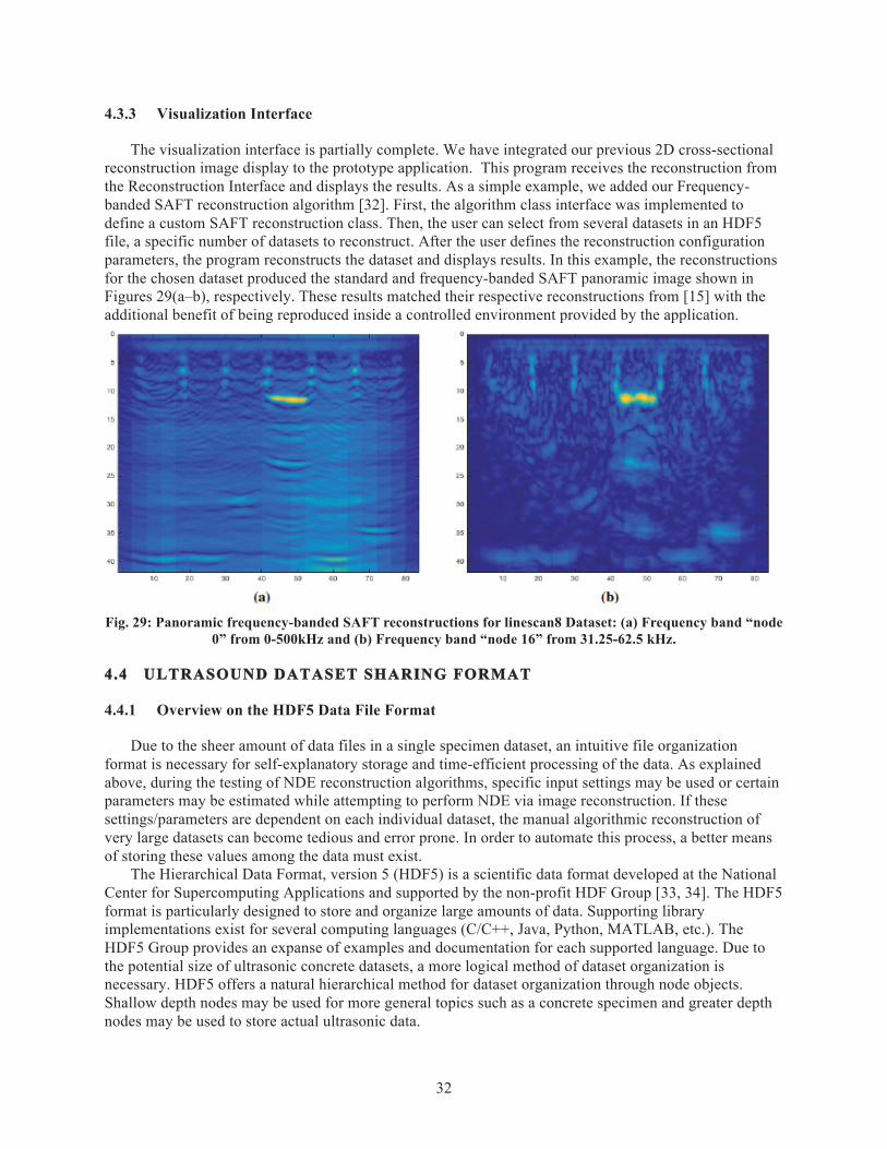
32

4.3.3 Visualization Interface

The visualization interface is partially complete. We have integrated our previous 2D cross-sectional reconstruction image display to the prototype application. This program receives the reconstruction from the Reconstruction Interface and displays the results. As a simple example, we added our Frequency-banded SAFT reconstruction algorithm [32]. First, the algorithm class interface was implemented to define a custom SAFT reconstruction class. Then, the user can select from several datasets in an HDF5 file, a specific number of datasets to reconstruct. After the user defines the reconstruction configuration parameters, the program reconstructs the dataset and displays results. In this example, the reconstructions for the chosen dataset produced the standard and frequency-banded SAFT panoramic image shown in Figures 29(a–b), respectively. These results matched their respective reconstructions from [15] with the additional benefit of being reproduced inside a controlled environment provided by the application.

Fig. 29: Panoramic frequency-banded SAFT reconstructions for linescan8 Dataset: (a) Frequency band “node

0” from 0-500kHz and (b) Frequency band “node 16” from 31.25-62.5 kHz.

44.4 ULTRASOUND DATASET SHARING FORMAT

4.4.1 Overview on the HDF5 Data File Format

Due to the sheer amount of data files in a single specimen dataset, an intuitive file organization format is necessary for self-explanatory storage and time-efficient processing of the data. As explained above, during the testing of NDE reconstruction algorithms, specific input settings may be used or certain parameters may be estimated while attempting to perform NDE via image reconstruction. If these settings/parameters are dependent on each individual dataset, the manual algorithmic reconstruction of very large datasets can become tedious and error prone. In order to automate this process, a better means of storing these values among the data must exist.

The Hierarchical Data Format, version 5 (HDF5) is a scientific data format developed at the National Center for Supercomputing Applications and supported by the non-profit HDF Group [33, 34]. The HDF5 format is particularly designed to store and organize large amounts of data. Supporting library implementations exist for several computing languages (C/C++, Java, Python, MATLAB, etc.). The HDF5 Group provides an expanse of examples and documentation for each supported language. Due to the potential size of ultrasonic concrete datasets, a more logical method of dataset organization is necessary. HDF5 offers a natural hierarchical method for dataset organization through node objects. Shallow depth nodes may be used for more general topics such as a concrete specimen and greater depth nodes may be used to store actual ultrasonic data.

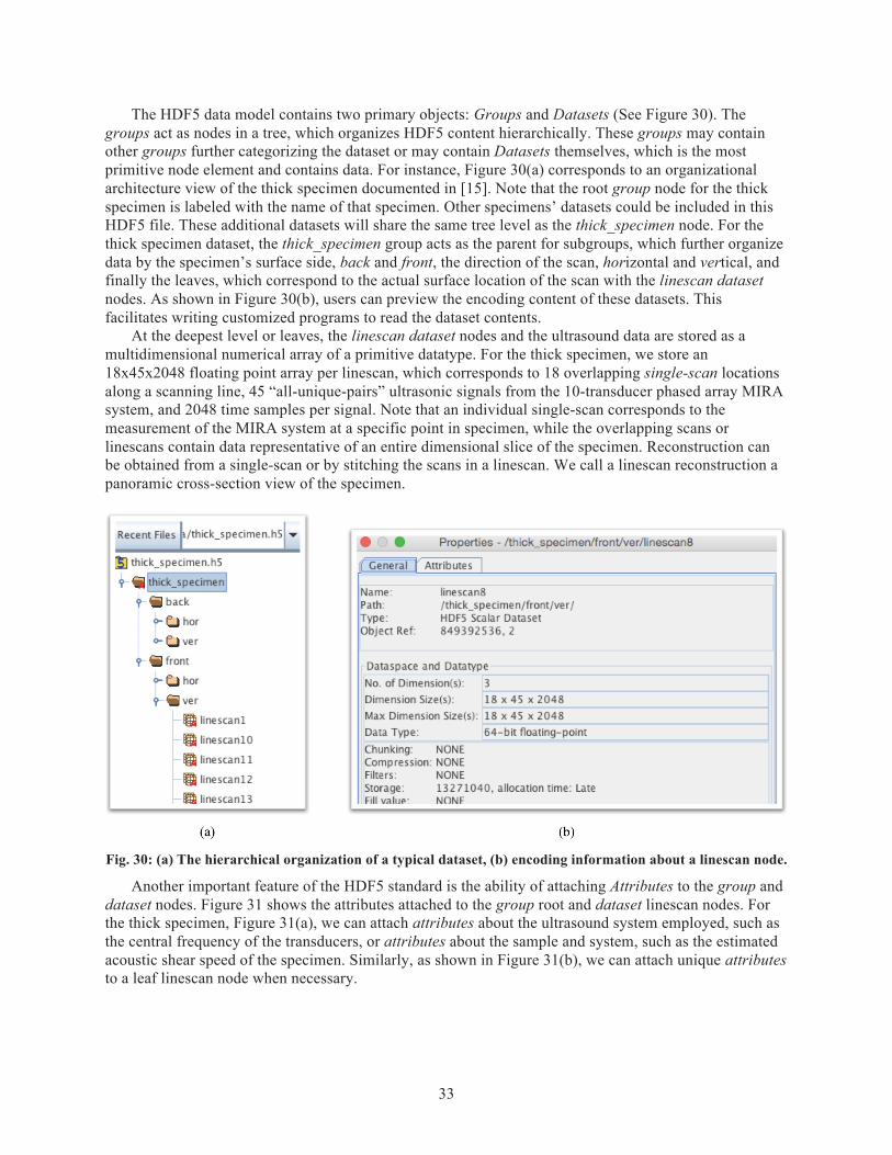
33

The HDF5 data model contains two primary objects: Groups and Datasets (See Figure 30). The groups act as nodes in a tree, which organizes HDF5 content hierarchically. These groups may contain other groups further categorizing the dataset or may contain Datasets themselves, which is the most primitive node element and contains data. For instance, Figure 30(a) corresponds to an organizational architecture view of the thick specimen documented in [15]. Note that the root group node for the thick specimen is labeled with the name of that specimen. Other specimens’ datasets could be included in this HDF5 file. These additional datasets will share the same tree level as the thick_specimen node. For the thick specimen dataset, the thick_specimen group acts as the parent for subgroups, which further organize data by the specimen’s surface side, back and front, the direction of the scan, horizontal and vertical, and finally the leaves, which correspond to the actual surface location of the scan with the linescan dataset nodes. As shown in Figure 30(b), users can preview the encoding content of these datasets. This facilitates writing customized programs to read the dataset contents.

At the deepest level or leaves, the linescan dataset nodes and the ultrasound data are stored as a multidimensional numerical array of a primitive datatype. For the thick specimen, we store an 18x45x2048 floating point array per linescan, which corresponds to 18 overlapping single-scan locations along a scanning line, 45 “all-unique-pairs” ultrasonic signals from the 10-transducer phased array MIRA system, and 2048 time samples per signal. Note that an individual single-scan corresponds to the measurement of the MIRA system at a specific point in specimen, while the overlapping scans or linescans contain data representative of an entire dimensional slice of the specimen. Reconstruction can be obtained from a single-scan or by stitching the scans in a linescan. We call a linescan reconstruction a panoramic cross-section view of the specimen.

Fig. 30: (a) The hierarchical organization of a typical dataset, (b) encoding information about a linescan node.

Another important feature of the HDF5 standard is the ability of attaching Attributes to the group and dataset nodes. Figure 31 shows the attributes attached to the group root and dataset linescan nodes. For the thick specimen, Figure 31(a), we can attach attributes about the ultrasound system employed, such as the central frequency of the transducers, or attributes about the sample and system, such as the estimated acoustic shear speed of the specimen. Similarly, as shown in Figure 31(b), we can attach unique attributes to a leaf linescan node when necessary.

34

Fig. 31: Examples of attributes assigned to (a) a specimen group and (b) a leaf linescan dataset.

44.5 DATASET FRAMEWORK CLOSING REMARKS

We have developed a prototype application built upon our envisioned HDF5 organizational architecture, to show that an HDF5-based framework is a valuable solution for furthering concrete NDE research by enabling and encouraging research collaboration. This scheme was chosen to allow an HDF5 file to be extended with new specimen data without causing conflict with other specimen datasets. In addition, the HDF5 hierarchical structure exhibits a natural, self-descriptive organization and may contain any local metadata necessary for image reconstruction or visualization.

Our application provides a controlled environment for data conversion and algorithm testing which facilitates the production of sharable, publishable, and reproducible data and results. We have demonstrated the effectiveness of the framework and application through the conversion of our own UTD proprietary data files and reconstruction with our own algorithms. The framework works well for moderately-sized rectangular concrete specimens, but could be expanded to support specimens of varying sizes and geometries. A natural expansion of our developing application would be to incorporate advanced data visualization tools for both the raw and reconstructed datasets.

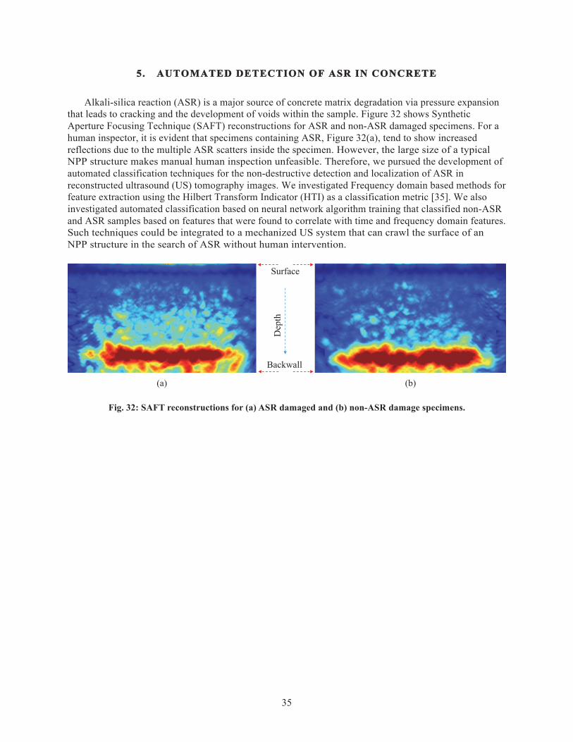
35

55. AUTOMATED DETECTION OF ASR IN CONCRETE

Alkali-silica reaction (ASR) is a major source of concrete matrix degradation via pressure expansion that leads to cracking and the development of voids within the sample. Figure 32 shows Synthetic Aperture Focusing Technique (SAFT) reconstructions for ASR and non-ASR damaged specimens. For a human inspector, it is evident that specimens containing ASR, Figure 32(a), tend to show increased reflections due to the multiple ASR scatters inside the specimen. However, the large size of a typical NPP structure makes manual human inspection unfeasible. Therefore, we pursued the development of automated classification techniques for the non-destructive detection and localization of ASR in reconstructed ultrasound (US) tomography images. We investigated Frequency domain based methods for feature extraction using the Hilbert Transform Indicator (HTI) as a classification metric [35]. We also investigated automated classification based on neural network algorithm training that classified non-ASR and ASR samples based on features that were found to correlate with time and frequency domain features. Such techniques could be integrated to a mechanized US system that can crawl the surface of an NPP structure in the search of ASR without human intervention.

Fig. 32: SAFT reconstructions for (a) ASR damaged and (b) non-ASR damage specimens.

(a) (b)

Depth

Backwall

Surface

36

55.1 FREQUENCY DOMAIN METHODS AND CLASSIFICATION FEATURES

(a) (b)

(c) (d)

Fig. 33: FFT spectral analysis results of 4 representative cases.

The frequency content in the averaged A-scan data for representative non-ASR and ASR samples are presented in Figure 33 for both raw and smooth spectra and the most significant time period regimes are evident in this plot. Figures 33(a) and 33(b) represent the raw spectral data while Figures 33(c) and 33(d) represent the smoothed data. R is the ratio non ASR:ASR of summed FFT amplitudes within regions demarcated by the vertical green lines. As depicted, characteristic peaks within certain bands are summarized in Table 1. The first regime is the cross-talk zone that encompasses the first 60 µs time-shift period. The second regime is the backwall reflectance zone that follows the cross-talk regime and encompasses the rest of the signal acquisition time duration. A closer examination of each of these regimes and zones follows.

Table 2: Averaged values for all 45 probe pair combinations for the most representative non-ASR and ASR samples based on HTI-value classification. R=(nASR/ASR).

Δ Δ

Δ

Δ

5-100 1.0135 0.0135 6100-200

1.6037 0.6037 1

200-260

1.1775 0.1775 4

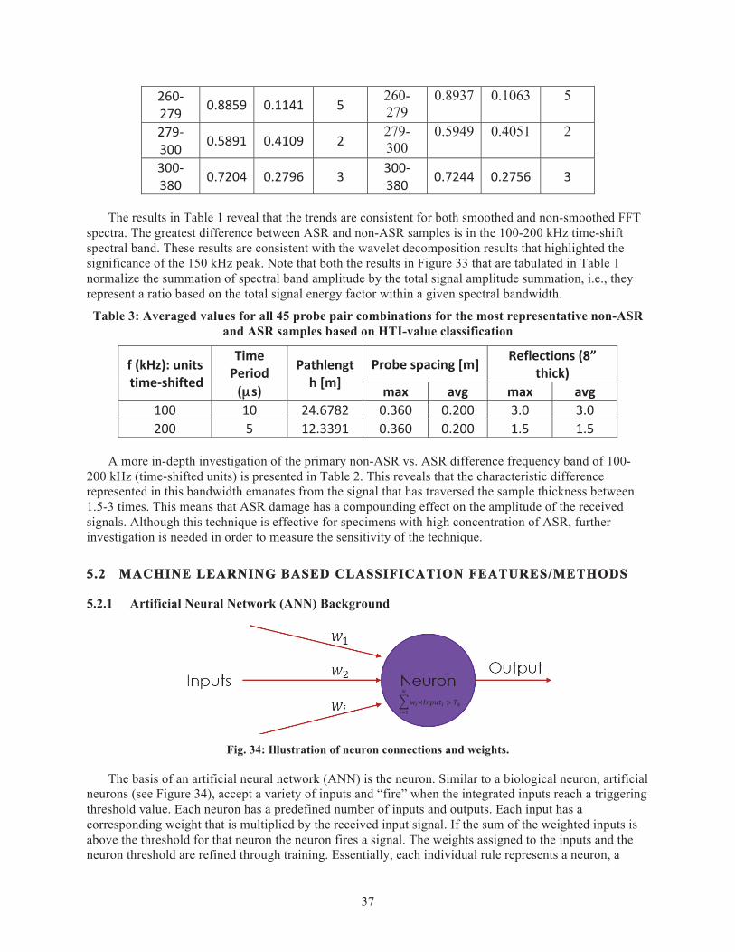
37

260-279

0.8937 0.1063 5

279-300

0.5949 0.4051 2

The results in Table 1 reveal that the trends are consistent for both smoothed and non-smoothed FFT spectra. The greatest difference between ASR and non-ASR samples is in the 100-200 kHz time-shift spectral band. These results are consistent with the wavelet decomposition results that highlighted the significance of the 150 kHz peak. Note that both the results in Figure 33 that are tabulated in Table 1 normalize the summation of spectral band amplitude by the total signal amplitude summation, i.e., they represent a ratio based on the total signal energy factor within a given spectral bandwidth.

Table 3: Averaged values for all 45 probe pair combinations for the most representative non-ASR and ASR samples based on HTI-value classification

A more in-depth investigation of the primary non-ASR vs. ASR difference frequency band of 100-200 kHz (time-shifted units) is presented in Table 2. This reveals that the characteristic difference represented in this bandwidth emanates from the signal that has traversed the sample thickness between 1.5-3 times. This means that ASR damage has a compounding effect on the amplitude of the received signals. Although this technique is effective for specimens with high concentration of ASR, further investigation is needed in order to measure the sensitivity of the technique.

55.2 MACHINE LEARNING BASED CLASSIFICATION FEATURES/METHODS

5.2.1 Artificial Neural Network (ANN) Background

Fig. 34: Illustration of neuron connections and weights.

The basis of an artificial neural network (ANN) is the neuron. Similar to a biological neuron, artificial neurons (see Figure 34), accept a variety of inputs and “fire” when the integrated inputs reach a triggering threshold value. Each neuron has a predefined number of inputs and outputs. Each input has a corresponding weight that is multiplied by the received input signal. If the sum of the weighted inputs is above the threshold for that neuron the neuron fires a signal. The weights assigned to the inputs and the neuron threshold are refined through training. Essentially, each individual rule represents a neuron, a

μμ

38

combination of two rules represents a neural connection, and each serial combination of rules between the original input(s) and the overall ANN output represents a layer. The neural connections can be layered, that is to say that the connections can be hidden from the original inputs and/or the overall ANN output.

Typically, the neurons and their layered connections are created via a training process where representative cases are provided as inputs to create internal sets of rules for classification. The ANN learning process entails the determination of the appropriate weighting of each neuron in order to achieve the correct classification of the known samples of the training dataset. After the training is accomplished, then other known samples not used in the original training dataset, i.e., the validation dataset, can then be run through the ANN, and the classification results can be compared to the true values to determine the classification error rate. If the classification error rate for the validation dataset does not meet an acceptable tolerance level, then more characteristic samples are needed to rebuild and retrain the ANN. Upon achieving an acceptable error rate tolerance level, then the ANN is then ready to be applied to unknown samples, i.e., test dataset, for classification.

A major strength of the use of ANN is robustness in the presence of noise, as the correct output can be achieved via the training process of adjusting neural weights, thus minimizing its impact. Fundamentally, an ANN is a non-linear process that utilizes numerous non-linear (i.e., multi-dimensional), multiple relationships (i.e., multi-variable) within the data to achieve a classification. This contrasts with a linear method that employs a few well-defined linearly-related variables, and is thus inherently susceptible to noise. An underlying requirement for ANN success is the use of a sufficient number of well demarcated samples for training. ANN performance directly correlates to the quality of the training dataset. A notable downside of employing ANN is that the practical and/or physical basis for a given rule (i.e., neuron) or result (i.e., output) is not readily obvious. At times, this makes it difficult to achieve meaningful insights.

5.2.2 Development of ANN Algorithm/Method for ASR Detection

Fig. 35: Visualization of the implemented network.

For the specific application of ASR detection, with robustness to noise in mind, we developed an ANN based automated classification algorithms for non-ASR vs. ASR samples. A single input (an A-scan from a transducer pairing) is passed to ten neurons, whose output is then weighted and then summed to predict the classification label as damaged or undamaged. The training dataset consisted of the raw A-scan signals of the MIRA 45 transducer pairing combinations from previously classified representative samples (i.e., ground truth). As shown in Figure 35, a single-layer ANN, with ten interior neurons and one output neutron, were then used to define an ANN classification based on their appropriate weighting to ensure the accurate prediction of non-ASR and ASR ground truth samples used for the training.

39

Fig. 36: Confusion matrices for the data set in four categories: training set, validation set, testing set, and total.

For the training set, we used data from one non-damaged concrete sample—the Nefertiti specimen. All six regions of the specimen were included in the dataset. For ASR damage data, we used two specimens—the Ramses and Cleopatra specimens [35]. For the Ramses and Cleopatra specimens, we included the odd and even positions, respectively. The complete dataset was then randomly subdivided into three subsets: 70% training, 15%, validation and 15% testing datasets. The ANN receives a US time series and classifies the signal as 0 for undamaged, 1 for damaged. The Confusion matrix in Figure 36 summarizes the results for our training and testing. The algorithm correctly classified the testing dataset more than 95% of the time.

It was observed that false positives (i.e., classifying a healthy specimen as damaged) are below half of a percent, while there is an order magnitude increase in false negatives (i.e., classifying a damaged specimen as healthy). This increase in false negatives may be due to mislabeling of the ground truth data. Recall that the ANN considers each transducer pairing time series as a sample. This may be problematic since known classification labeling is at the US system position level and not at the level of each time series. In other words, every pairing is labeled with the same classification label even though each pairing traces a different path through the sample. It is possible for ASR damage to be present in a scan position, but not in the path of a specific transducer pairing. Consequently, the training datasets were regrouped by transducer pair distance.

40

Fig. 37: Size of dataset for each of the nine possible probe-space pairings and the ANN prediction error.

The measurement instrument, a phased array US system with 10 effective transducers, has a transducer pitch (i.e., transducer center-to-center distance) of 40mm. The left axis in Figure 32 shows the number of samples available for each corresponding transducer pair distance. Note that for the maximum transducer pair distance—i.e., the transducers located at the periphery of the system—there are only 132 available samples from our specimens, while for the shortest distance there are over a thousand samples. As mentioned above, ANN are excellent non-linear classifiers when the number of training samples is sufficiently high. This requirement does not hold for the maximum transducer pair distance.

The right axis in Figure 37 shows the error rate for each transducer pair distance set. The prediction error presented is based on the average results from 50 independent networks that were trained on different randomly selected training, validation and testing datasets. As such, the contribution of statistical errors has been minimized to achieve a better comparison between pairings. Still, note that the error stays below 5% for all distances apart from the group with for the lowest available samples—the maximum pairing distance. Therefore, the results for this group should be discarded, as data from more specimens is required. However, this may explain the increase in the number of false negatives in the overall tests.

41

5.2.3 Extracting meaningful insights from ANN algorithm/method for ASR detection

Fig. 38: Weights of each neuron in the network after training on the specified dataset.

The results of the ANN weightings for each of the aforementioned pre-treatments are presented in Figure 38 with each colored line representing an individual neuron. A few insights are revealed from these plots. First, the networks do not diverge in amplitudes for the independent treatments, but instead exhibit similarities for various epochs in the time series, i.e., time domain features. In particular, the weightings for the networks of the original raw and normalized signals exhibit the same pattern, with strong weights in the region containing the cross-talk and the backwall reflection signals. They also share significant weighting of the second reflection signal that is in the vicinity of 400µs. Therefore, the experiments above were repeated for time series samples with high backwall reflection likelihood.

42

Fig. 39: Confusion matrices for the dataset in four categories: training set, validation set, testing set, and total.

Figure 39 shows the classification error rates when using the original and post-processed data for training. The data set consisted of the initial signal, the backwall signal, the derivative of the signal, and normalized signal. The post-processed data results were grouped in three groups: the derivative of the raw time series, the standard score normalized time series, and the truncated time series that was selected for backwall reflected samples. All results were comparable, with best ANN classification performance when the network was trained with the normalized signals.

55.3 AUTOMATED DETECTION OF ASR CLOSING REMARKS

We have documented two independent techniques for the automated detection of ASR in concrete specimens. From both methods, the ANN technique shows great potential with classification accuracy above 95%. Further assessment of these techniques should be performed with a larger set of specimens in order to confirm and validate the results presented in this report. Note that these approaches are extensible to the detection of additional reinforced, thick concrete defects and damage. .

43

66. CONCLUSION

Given the age of most NPPs in the United States, it is critical to develop NDE techniques to assess the health of their concrete safety structures. To address these needs and challenges, advanced reconstruction techniques have been assessed using a specially fabricated representative NPP structure specimen with intentional embedded defects.

This report documents our efforts for the past year. The effort was split in four research areas: 1) Comparative study between traditional SAFT and FBD SAFT for concrete specimen with and without Alkali-Silica Reaction (ASR) damage, 2) improvement of our Model-Based Iterative Reconstruction (MBIR) for thick reinforced concrete [6], 3) development of a universal framework for sharing, reconstruction, and visualization of ultrasound NDE datasets, and 4) application of machine learning techniques for automated detection of ASR damaged concrete. Our comparative study between FBD and traditional SAFT reconstruction images shows a clear difference between images of ASR and non-ASR specimens. In particular, the first harmonic shows an increased contrast and sensitivity to ASR damage. For MBIR, we show the superiority of model-based techniques over delay and sum techniques such as SAFT. Improvements include elimination of artifacts caused by direct arrival signals, and increased contrast and Signal to Noise Ratio. For the universal framework, we document a format for data storage based on the HDF5 file format, and also propose a modular Graphic User Interface (GUI) for easy customization of data conversion, reconstruction, and visualization routines. Finally, we developed two techniques for ASR automated detection. The first technique is based on an analysis of the frequency content using Hilbert Transform Indicator (HTI) and the second technique employees Artificial Neural Network (ANN) techniques for training and classification of ultrasound data as ASR or non-ASR damaged classes. The ANN technique shows great potential with classification accuracy above 95%. These approaches are believed to be extensible to the detection of additional reinforced, thick concrete defects and damage.

Future investigation will be directed to the refinement of our universal framework and the collection and analysis of data from large thick concrete specimens affected by ASR – the University of Tennessee ASR specimens and the NIST specimen planned for FY2017. As we incorporate new datasets to our NDE program, we will enhance the current framework as needed. In addition, we plan to develop ASR measurements techniques that highly correlates with the visual appearance of the damage in the reconstruction images – even detecting ASR damage prior to any visible surface damage. Important improvements are needed to the current MBIR propagation model. We need to upgrade the current linear model to a non-linear model that address the attenuation of impedance differences for the reflected path. Finally, we will further assess the performance of the HTI and ANN ASR classification techniques with a larger dataset of ASR damaged specimens to determine which technique is most appropriate for concrete structures used in NPPs. Additionally, with the development of the ANN technique, additional data will be collected on the NPP specimen at the University of Minnesota varying various collection parameters to determine if the detection of defects can be improved using ANN.

44

45

77. REFERENCES

[1] J. I. Braverman, C. A. Miller, B. R. Ellingwood, D. J. Naus, C. H. Hofmayer, P. Bezler, and T. Y.

Chang, “Structural performance of degraded reinforced concrete members,” in Transaction 17th International Conference on Structural Mechanics, March 2001.

[2] L. J. Bond, "Old Reactors, New Tricks," IEEE Spectrum 49(8), 30–35 (2012).

[3] D. A. Clayton K. Hoegh, L. Khazanovich, and M. S. Hileman, “Preliminary Conceptual Design of Thick Concrete Nondestructive Evaluation Specimen,” ORNL/TM-2014/136, Oak Ridge National Laboratory, 2014.

[4] D. A. Clayton, K. Hoegh, and L. Khazanovich, “Thick Concrete Specimen Construction, Testing, and Preliminary Analysis,” ORNL/TM-2015/72, Oak Ridge National Laboratory, 2015.

[5] H. Almansouri, D. Clayton, R. Kisner, Y. Polsky, C. Bouman and H. Santos-Villalobos, “Development of acoustic model-based iterative reconstruction technique for thick-concrete imaging,” in AIP Conference Proceedings Review of Progress in Quantitative Nondestructive Evaluation (QNDE), July 2015.

[6] D. J. Naus, C. B. Oland, B. R. Ellingwood, C. J. Hookham and H. L. Graves III, "Summary and conclusions of a program addressing aging of nuclear power plant concrete structures," Nuclear Engineering and Design, vol. 194, no. 1, pp. 73-96, November 1999.

[7] D. J. Naus, C. B. Oland and E. G. Arndt, "Ageing management of safety-related concrete structures to provide improved bases for continuing the service of nuclear power plants," Materials and Structures, vol. 24, no. 4, pp. 308-316, 1991.

[8] Dwight A. Clayton, Cyrus M. Smith, Christopher Ferraro, Jordan Nelson, Lev Khazanovich, Kyle Hoegh, Satish Chintakunta, John Popovics, Hajin Choi, and Suyun Ham, “Evaluation of Ultrasonic Techniques on Concrete Structures,” ORNL/TM-2013/430, Oak Ridge National Laboratory, 2013.

[9] F. Schubert and R. Marklein, "Ten lectures on impact-echo," Journal of Nondestructive Evaluation, vol. 27, no. 1-3, pp. 5-21, 2008.

[10] J. Zhu and J. S. Popovics, "Imaging concrete structures using air-coupled impact-echo," Journal of Engineering Mechanics, vol. 133, no. 6, pp. 628-640, 2007.

[11] G. Gargour, M. Gabrea, V. Ramachandran and J. M. Lina, "A short introduction to wavelets and their applications," Circuits and Systems Magazine, vol. 9, no. 2, pp. 57-68, June 2009.

[12] O. Rioul and M. Vetterli, "Wavelets and signal processing," Signal Processing Magazine, vol. 8, no. 4, pp. 14-38, October 1991.

[13] I. Daubechies, "Ten lectures on Wavelets," in Society for Industrial Applied Mathematics (SIAM), Philadelphia, 1992.

46

[14] A. P. Albright and D. A. Clayton, "The benefits of using time-frequency analysis with synthetic aperture focusing technique," in Review of Progress Quantitative Nondestructive Evaluation, Minneapolis, 2015.

[15] D. A. Clayton, A. Barker, H. Santos-Villalobos, A. Albright, K. Hoegh and L. Khazanovich, "Nondestructive Evaluation of Thick Concrete Using Advanced Signal Processing Techniques," Oak Ridge National Laboratory, Oak Ridge, 2015.

[16] Z. Shao, L. Shi, Z. Shao, and J. Cai, Review of Scientific Instruments 82, p. 073708 (2011).

[17] B. J. Engle, J. L. W. Schmerr, and A. Sedov, AIP Conference Proceeding 1581, p. 49 (2014).

[18] G. Dobie, S. G. Pierce, and G. Hayward, NDT and E International 58, 10–17 (2013).

[19] Z. Yu, J. Thibault, C. Bouman, K. Sauer, and J. Hsieh, IEEE Transactions on Image Processing 20, 161–175, January (2011).

[20] M. E. Kamasak, C. A. Bouman, E. D. Morris, and K. Sauer, IEEE Transactions on Medical Imaging 24, 636–650, May (2005).

[21] Z. H. Levine, A. J. Kearsley, and J. G. Hagedorn, J. Res. Nat. Inst. Stand. Technol. 11, 411–417, November (2006).

[22] M. Katsura, I. Matsuda, M. Akahane, J. Sato, H. Akai, K. Yasaka, A. Kunimatsu, and K. Ohtomo, European Radiology 22, p. 1613-1623 (2012).

[23] S. Boudabbous, D. Arditi, E. Paulin, A. Syrogiannopoulou, C. Becker, and X. Montet, American Journal of Roentgenology 205, p. 380-385 (2015).

[24] C. Bouman, Model Based Image Processing, 1st ed. (Purdue University, 2013).

[25] Q. Wang and G. Ren, IEEE Transactions on Wireless Communications 14, 2778–2787, May (2015).

[26] Z. Haiyan, S. Xiuli, Q. Xuerui, F. Shixuan, L. Xiao, and L. Donghui, “Lamb wave tomography combining simulated annealing and simultaneous iterative reconstruction technique,” in Microwave Conference (2008), pp. 741–744.

[27] S. Venkatakrishnan, L. Drummy, M. Jackson, M. D. Graef, J. Simmons, and C. Bouman, IEEE Transactions on Image Processing 22, 4532–4544, November (2013).

[28] S. J. Norton and M. Linzer, IEEE Transactions on Biomedical Engineering BME-28, 202–220, February (1981).

[29] A. Kak and K. A. Dines, IEEE Transactions on Biomedical Engineering BME-25, 321–344, July (1978).

[30] B. E. Treeby and B. T. Cox, J. Biomed. Opt. 14, p. 021314 (2010).

[31] Acoustic Control Systems (ACSYS), Ultrasonic Tomograph for Imaging of Concrete Structures A1040 MIRA, http://www.acsys.ru/eng/production/detail/a1040-mira/ (2016).

[32] A. Albright and D. Clayton, “The benefits of using time-frequency analysis with synthetic aperture focusing technique,” in 41st Annual Review of Progress in Quantitative Nondestructive Evaluation: Volume 34, Vol. 1650 (AIP Publishing, 2015), pp. 94–103.

47

[33] The HDF Group, Hierarchical Data Format, Version 5, http://www.hdfgroup.org/HDF5 (1997-2016).

[34] National Center for Supercomputing Applications, National Center for Supercomputing Applications Web Page, http://www.ncsa.illinois.edu/ (July 2015).

[35] D. A. Clayton, L. Khazanovich, and Lucio Salles, “Linear Array Ultrasonic Test Results from Alkali-Silica Reaction (ASR) Specimens”, ORNL/TM-2016/159, Oak Ridge National Laboratory, 2016.

Documents

Evaluation of Advanced Signal Processing Techniques to