Evaluation of a new tool for use in association mapping

Structure

Reinhard Simon, 2002/10/29

Structure 2.0

http://pritch.bsd.uchicago.edu

Pritchard JK, Stephens M, Donelly P (2000): Inference of population structure using multilocus genotype data. Genetics, 155: 945-959

Software

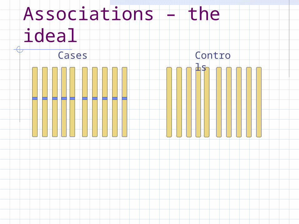
Associations – the ideal Cases Control

s

Test for association

A diploid locus: Pearsons Chi-square test

*

28)(AA

oaoa nn

mmmqq

Example: Contingency table

Frequency of Total # of alleles (diploid)

Alleles A A*

Cases qa 1-qa 2ma

Controls

qo 1-qo 2mo

total nA nA* 2m

Associations – the less ideal

Cases Controls

Associations – simple admixture

Cases Controls

Associations – admixture complications

Cases Controls

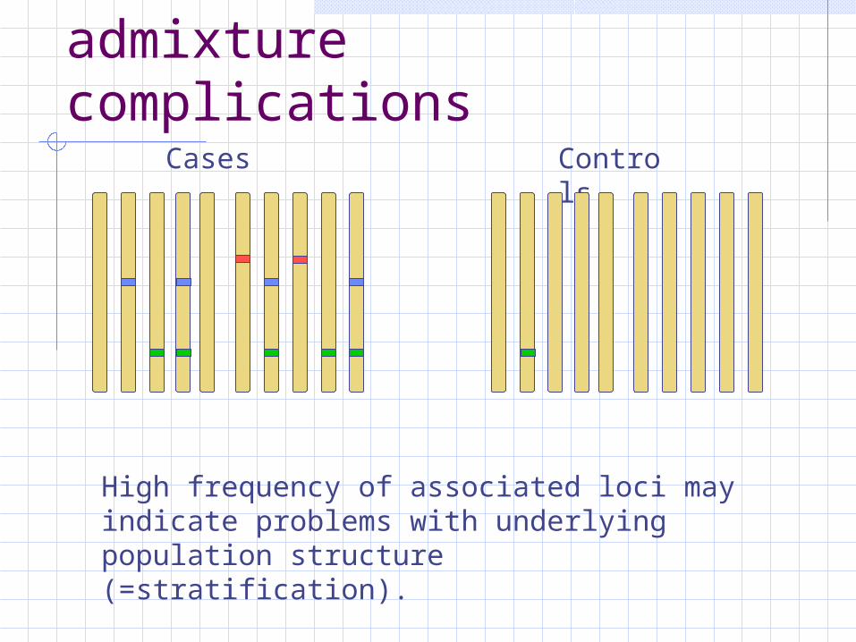
Associations – admixture complications

Cases Controls

High frequency of associated loci may indicate problems with underlying population structure (=stratification).

Associations – accounted for

Cases Controls

Questions

• Is there a stratification?

• If so: - how many subpopulations- which individual belongs to which

subpopulation

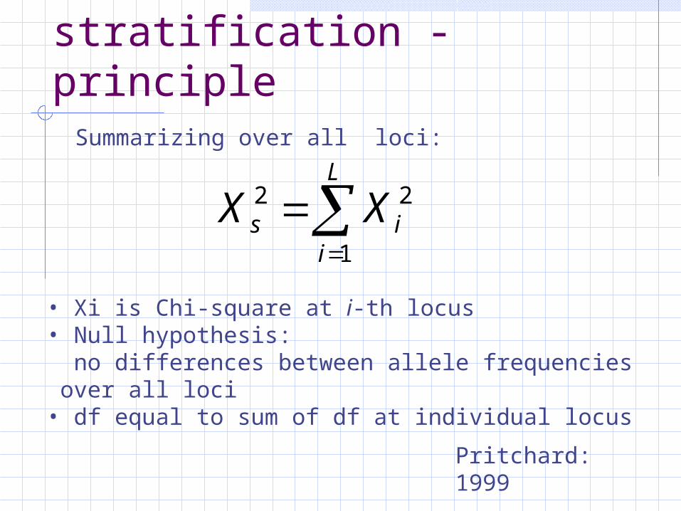
Test for stratification - principle

Summarizing over all loci:

L

iis XX

1

22

• Xi is Chi-square at i-th locus• Null hypothesis: no differences between allele frequencies over all loci• df equal to sum of df at individual locus

Pritchard: 1999

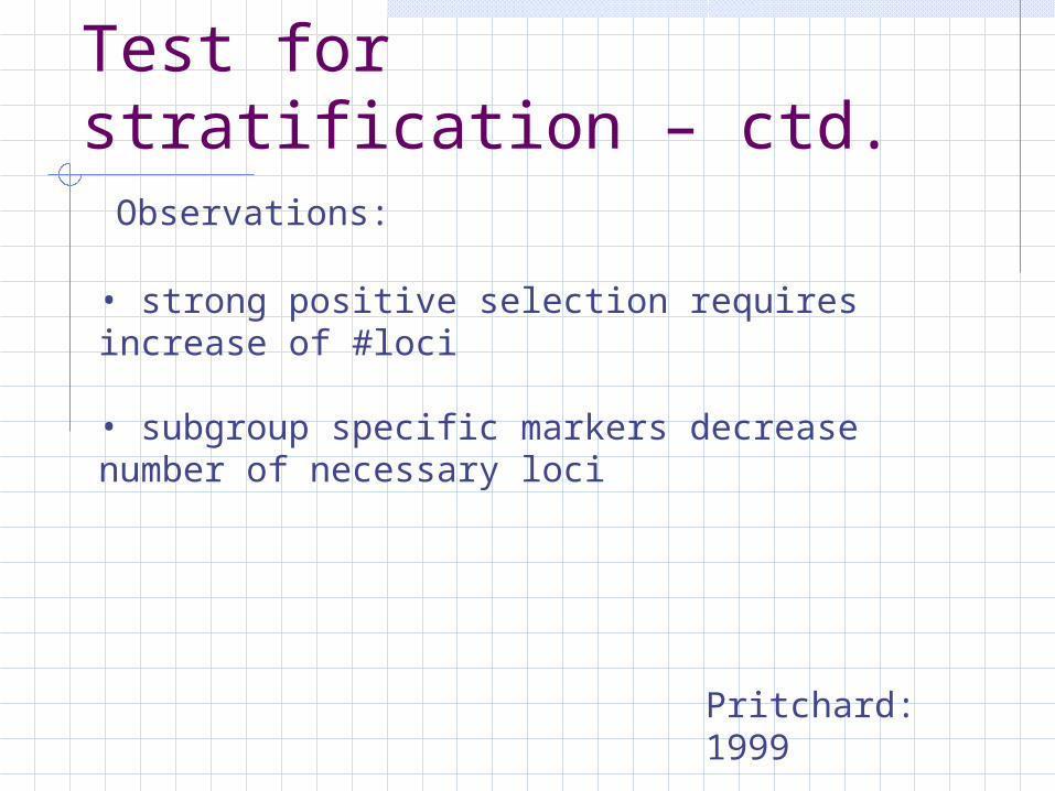
Test for stratification – ctd.Observations:

• strong positive selection requires increase of #loci

• subgroup specific markers decrease number of necessary loci

Pritchard: 1999

How to group individuals?

Based on distance measures Based on models

Pair wise distance measures

Jaccard

Nei & Li

Sokal & Michener

Model based Bayesian inference

• Bayesean statistics: Uncertainty is modeled using probabilities

• probability statements are made about model parameters

Advantages:

• very general framework

• assumptions are made explicit and are quantified

Bayesian inference – how?

Bayesian inference centers on the posterior distribution p(theta|X), e.g.a genetic model of the distribution of allele frequencies However, analytic evaluation is seldom possible ....

Bayesian inference - methods

Alternatives:

Numerical evaluation approximation simulation, e.g. Markov Chain Monte Carlo Methods

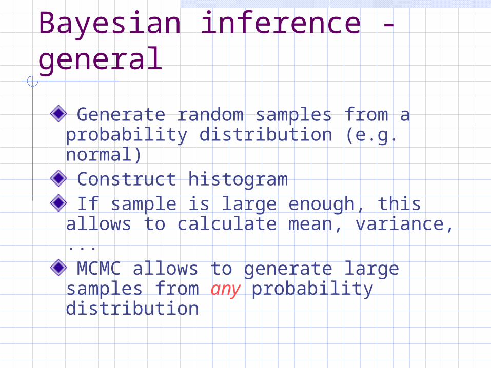
Simulation methods for Bayesian inference - general

Generate random samples from a probability distribution (e.g. normal) Construct histogram If sample is large enough, this allows to calculate mean, variance, ... MCMC allows to generate large samples from any probability distribution

Markov Chain behaviour

• Reaches an equilibrium (basic MCMC theorem) and

• the present state depends only on the preceding: “The future depends on the past only through the present.”

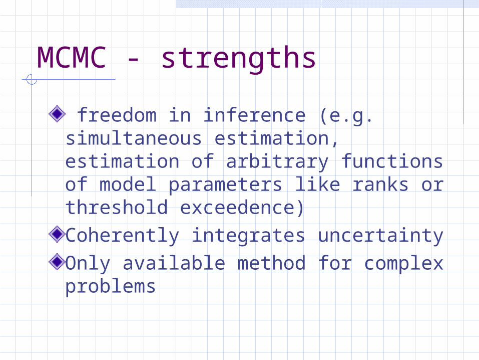
MCMC - strengths

freedom in inference (e.g. simultaneous estimation, estimation of arbitrary functions of model parameters like ranks or threshold exceedence)Coherently integrates uncertaintyOnly available method for complex problems

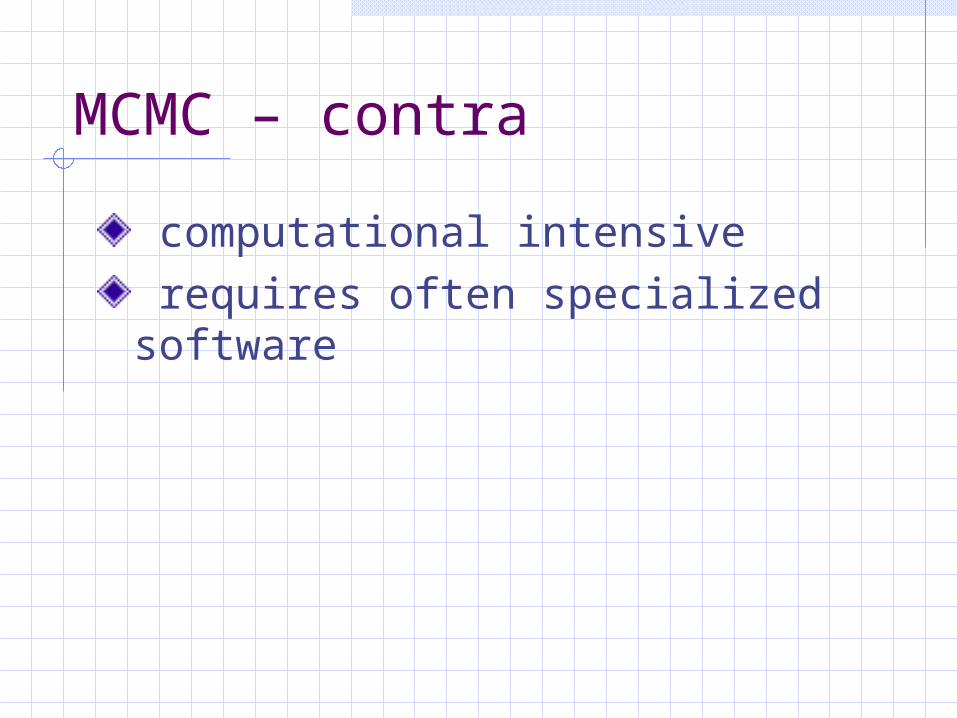
MCMC – contra

computational intensive requires often specialized software

Inferring population structure

X = genotypes of sampled invidualsunknown:Z = population of originP = allele frequencies in all populationsQ = proportion of genome that originates from population k

Pr(Z, P, Q|X) ~ Pr(Z) * Pr(P) * Pr(Q) * Pr(X|Z,P,Q)

Solution:Using MCMC for Bayesian inference;simultaneous estimation of Q, Z and P.

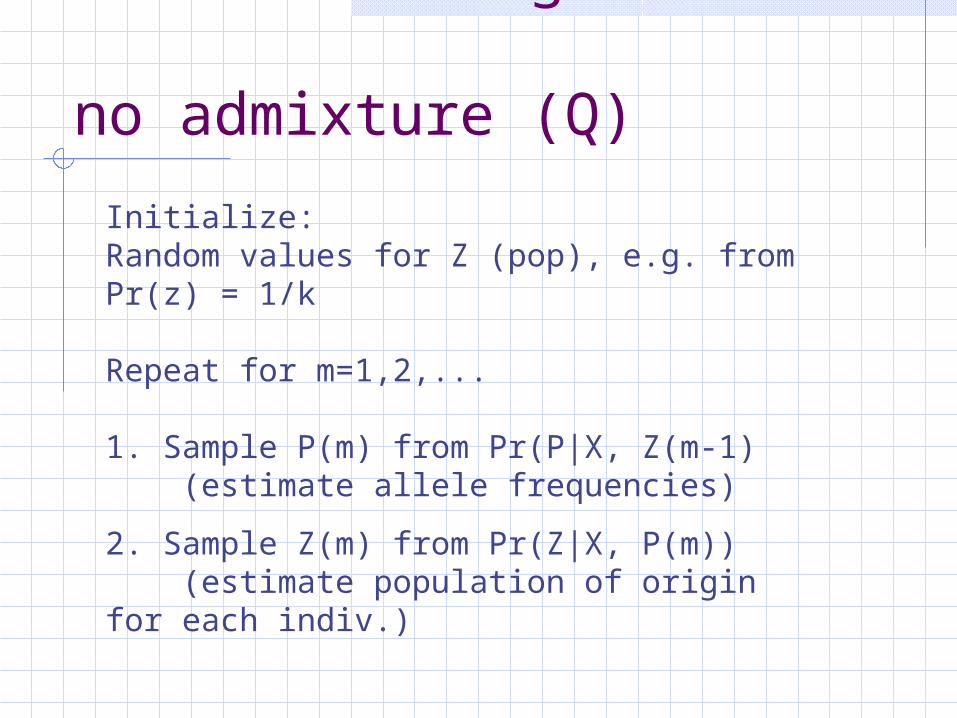
Basic MCMC algorithm – no admixture (Q)

Initialize:Random values for Z (pop), e.g. from Pr(z) = 1/k

Repeat for m=1,2,...

1. Sample P(m) from Pr(P|X, Z(m-1) (estimate allele frequencies)

2. Sample Z(m) from Pr(Z|X, P(m)) (estimate population of origin for each indiv.)

Basic MCMC algorithm – with admixture (Q)

Initialize:Random values for Z (pop), e.g. from Pr(z) = 1/k

Repeat for m=1,2,...

1. Sample P(m), Q(m) from Pr(P, Q|X, Z(m-1) (estimate allele frequencies)

2. Sample Z(m) from Pr(Z|X, P(m), Q(m))

3. Update alpha (admixture proportion)

Program – parameters: MCMC

Program – parameters: Q

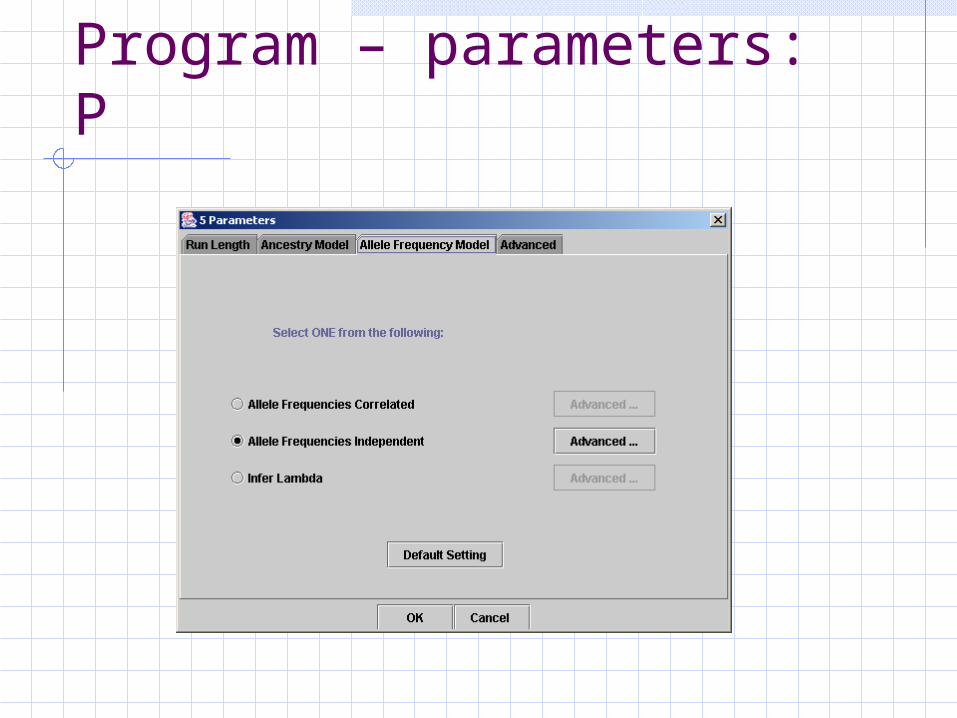
Program – parameters: P

Program – parameters: Z, K

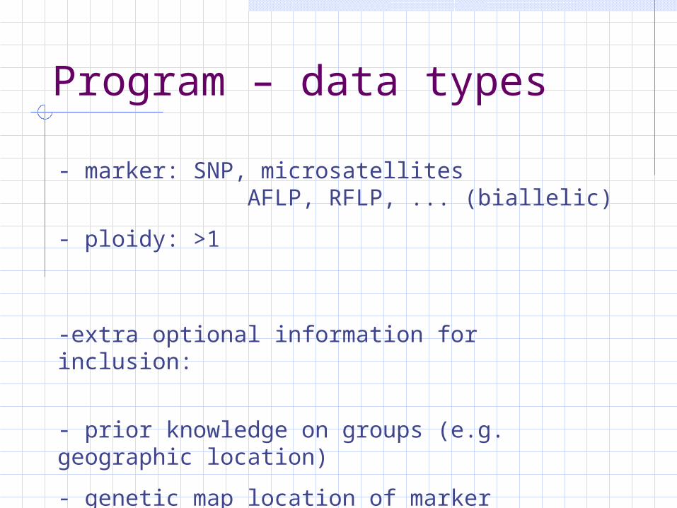
Program – data types

- marker: SNP, microsatellites AFLP, RFLP, ... (biallelic)

- ploidy: >1

-extra optional information for inclusion:

- prior knowledge on groups (e.g. geographic location)

- genetic map location of marker

Program – data format

Example – S.t. tuberosum vs andigena

Other:1st 30 genotypes from tuberosum

2nd 20 genotypes from andigena

Example – S.t. tuberosum vs andigenaPNA:

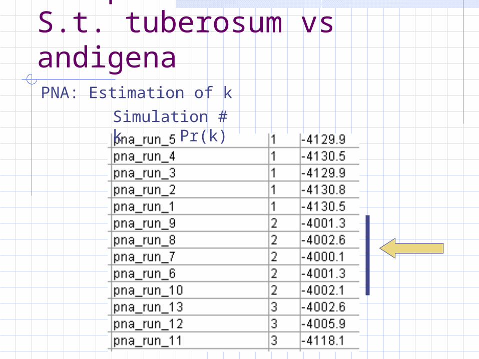
Example – S.t. tuberosum vs andigenaPNA: Estimation of k

Simulation # k Pr(k)

Example – S.t. tuberosum vs andigenaPNA: assignment

1 = tbr; 2 = adggenotypes #31-#3: adg from Indiagenotype #49: adg from Ecuador

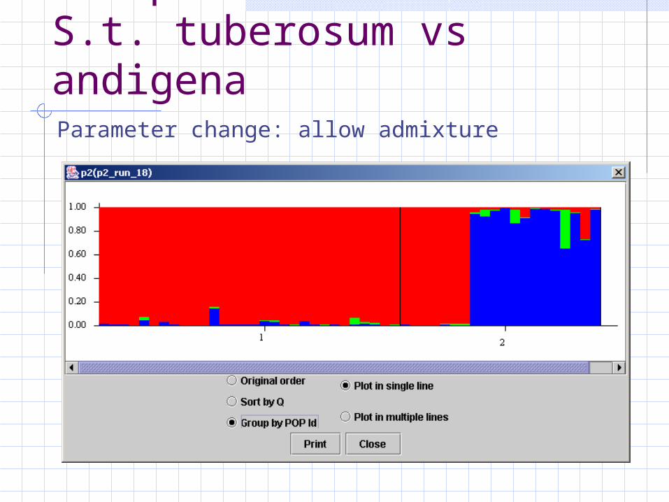
Example – S.t. tuberosum vs andigenaParameter change: allow admixture

Ancestry Model Info Use Admixture Model * Infer Alpha * Initial Value of ALPHA (Dirichlet Parameter for Degree of Admixture): 1.0

* Use Same Alpha for all Populations * Use a Uniform Prior for Alpha ** Maximum Value for Alpha: 10.0 ** SD of Proposal for Updating Alpha: 0.025

Frequency Model Info

Allele Frequencies are Independent among Pops * Infer LAMBDA ** Use a Uniform Lambda for All Population ** Initial Value of Lambda: 1.0

Example – S.t. tuberosum vs andigenaParameter change: allow admixture

Example – S.t. tuberosum vs andigenaParameter change: allow admixture

sub1 sub2 sub345 Huaycha-ADG 0 2 : 0.012 0.002 0.985 (0.000,0.081) (0.000,0.011) (0.912,1.000)46 Huagalina-ADG 0 2 : 0.021 0.004 0.976 (0.000,0.135) (0.000,0.022) (0.854,1.000)47 Guincho-ADG 0 2 : 0.019 0.326 0.655 (0.000,0.113) (0.164,0.503) (0.449,0.829)48 Puca-ADG-BO 0 2 : 0.038 0.006 0.957 (0.000,0.267) (0.000,0.037) (0.729,1.000)49 Puna-ADG-EC 0 2 : 0.270 0.002 0.728 (0.000,1.000) (0.000,0.010) (0.000,1.000)50 Pellejo-ADG 0 2 : 0.011 0.007 0.983 (0.000,0.061) (0.000,0.049) (0.899,1.000)

Example – S.t. tuberosum vs andigenaParameter change: allow admixture

Example – andigena

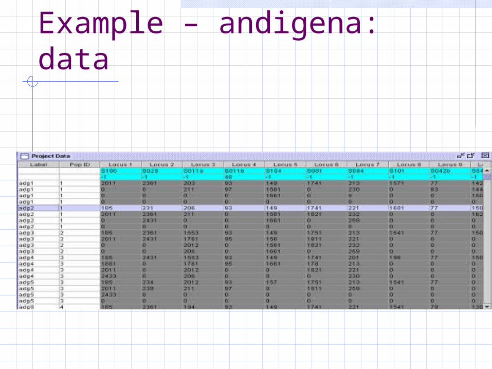
Example – andigena: data

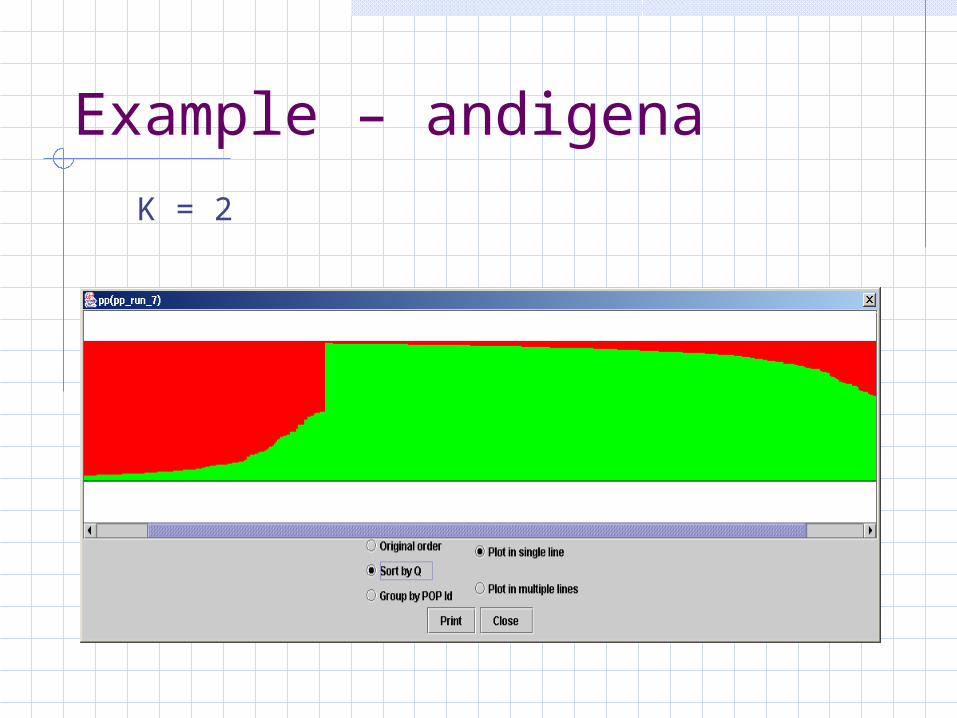
Example – andigena

K = 2

Example – andigenaK = 3

Example – andigenaK = 3

Example – andigena: genetic distance

K = 3

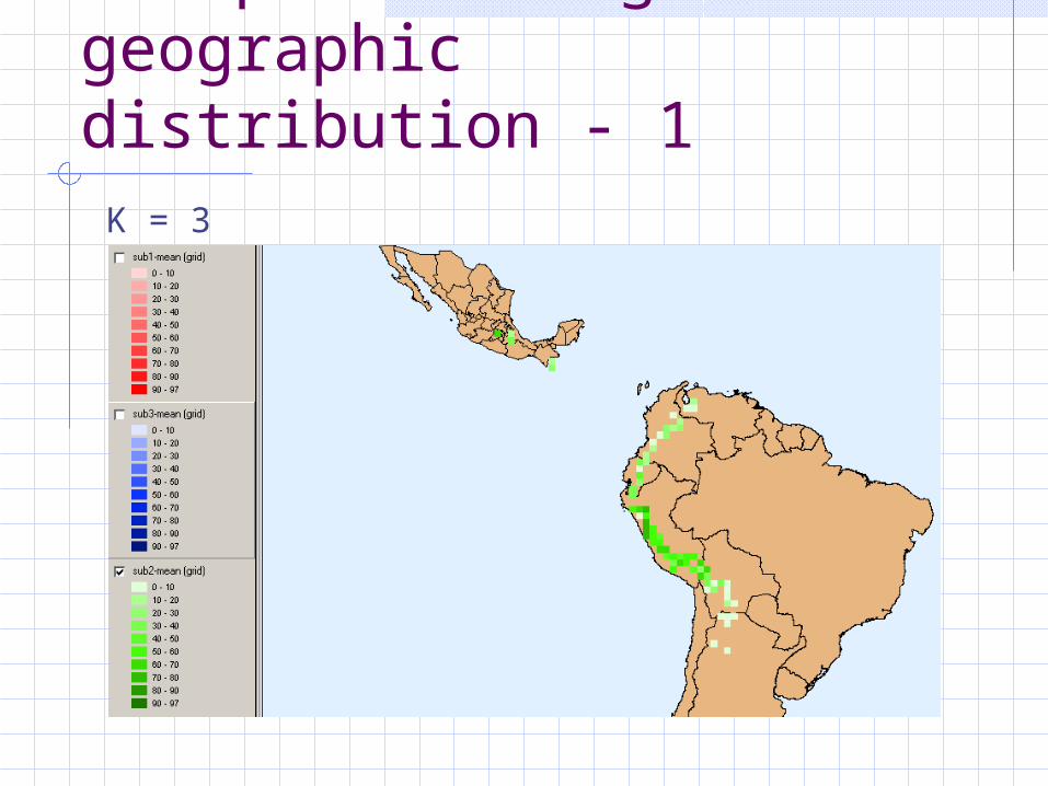
Example – andigena: geographic distribution - 1

K = 3

Example – andigena: geographic distribution - 2

K = 3

Example – andigena: geographic distribution - 3

K = 3

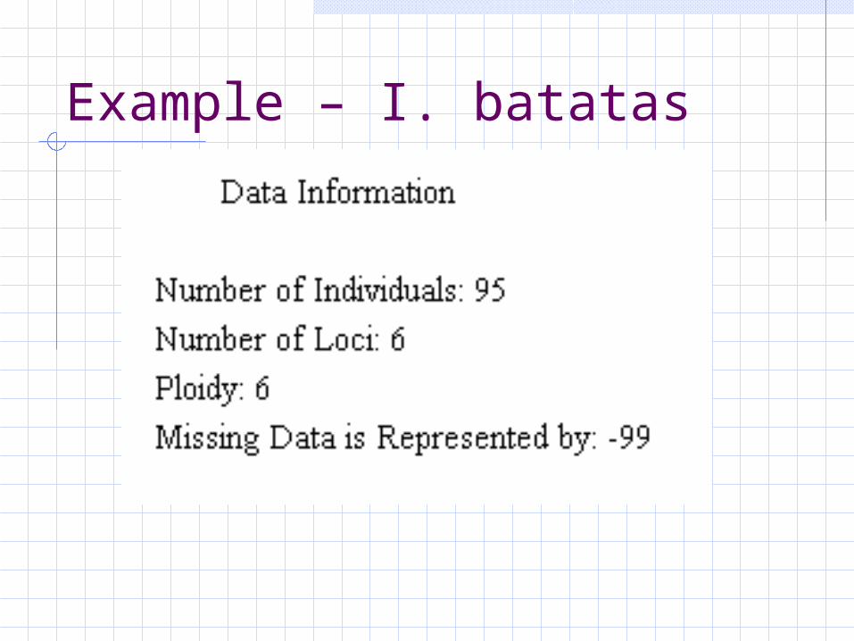
Example – I. batatas

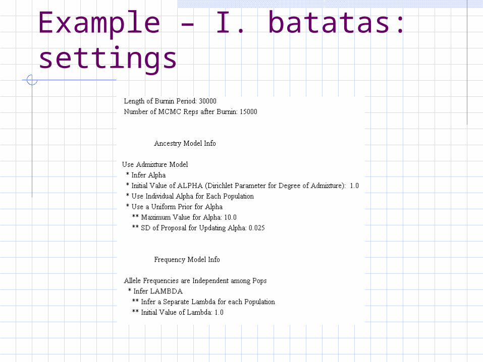
Example – I. batatas: settings

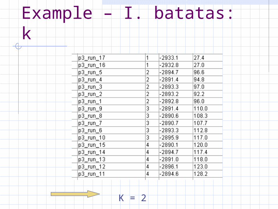
Example – I. batatas: k

K = 2

Example – I. batatas: k = 2

1=PAN, 2=HON, 3=GTM, 4=NIC, 5=MEX, 6=COL, 7=VEN, 8=ECU, 9=PER

Example – I. batatas: k = 3

1=PAN, 2=HON, 3=GTM, 4=NIC, 5=MEX, 6=COL, 7=VEN, 8=ECU, 9=PER

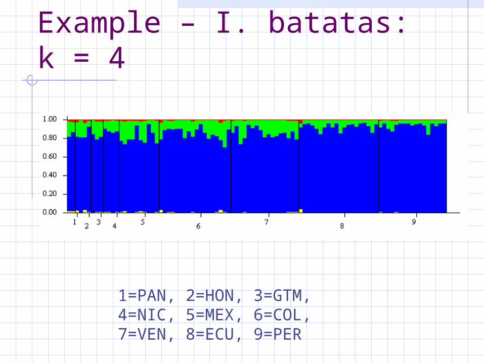
Example – I. batatas: k = 4

1=PAN, 2=HON, 3=GTM, 4=NIC, 5=MEX, 6=COL, 7=VEN, 8=ECU, 9=PER

Example – I. batatas: genetic distance

Example – S. paucissectum

Example – paucissectum: data

Example – paucissectum: configuration

Example – paucissectum: results: k =2

Example – paucissectum: results: k =3

Example – paucissectum: results: k =3

Example – paucissectum: results: k =4

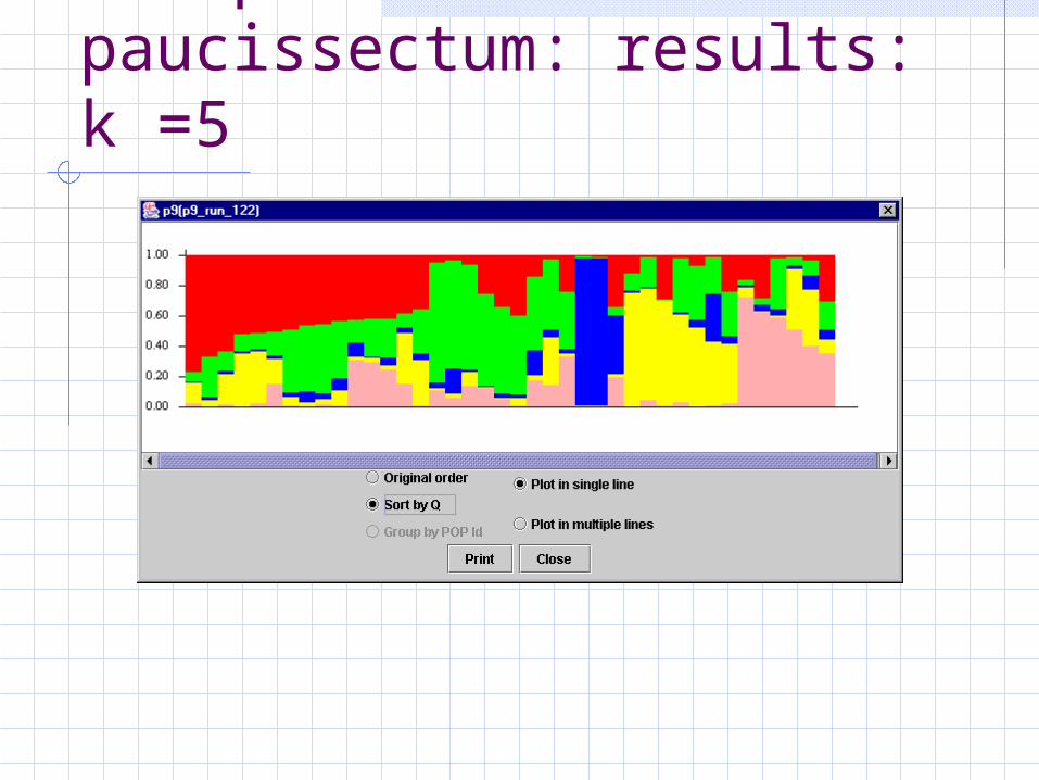
Example – paucissectum: results: k =5

Example – paucissectum: results: k =6

Summary

• The software was tested with population data from diploid, tetraploid and hexaploid species with microsatellite and biallelic marker

• The algorithm seems stable and delivers sensible results under a variety of settings

• Great advantage: assigns each individual a probability of being a member of a certain subgroup

Thanks for your attention!