Embed Size (px)
Citation preview
Evaluation of a 3D ReconstructionSystem Comprising Multiple
Stereo Cameras
DIPLOMARBEIT
zur Erlangung des akademischen Grades
Diplom-Ingenieur
im Rahmen des Studiums
Computational Intelligence
eingereicht von
Christian Kapeller, BSc.
Matrikelnummer 0225408
an der Fakultät für Informatik
der Technischen Universität Wien
Betreuung: Ao.Univ.-Prof. Dipl.-Ing. Mag. Dr. Margrit Gelautz
Wien, 13. November 2018
Christian Kapeller Margrit Gelautz
Technische Universität Wien
A-1040 Wien Karlsplatz 13 Tel. +43-1-58801-0 www.tuwien.ac.at

Evaluation of a 3D ReconstructionSystem Comprising Multiple
Stereo Cameras
DIPLOMA THESIS
submitted in partial fulfillment of the requirements for the degree of
Diplom-Ingenieur
in
Computational Intelligence
by
Christian Kapeller, BSc.
Registration Number 0225408
to the Faculty of Informatics
at the TU Wien
Advisor: Ao.Univ.-Prof. Dipl.-Ing. Mag. Dr. Margrit Gelautz
Vienna, 13th November, 2018
Christian Kapeller Margrit Gelautz
Technische Universität Wien
A-1040 Wien Karlsplatz 13 Tel. +43-1-58801-0 www.tuwien.ac.at


Erklärung zur Verfassung der
Arbeit
Christian Kapeller, BSc.
Hiermit erkläre ich, dass ich diese Arbeit selbständig verfasst habe, dass ich die verwen-deten Quellen und Hilfsmittel vollständig angegeben habe und dass ich die Stellen der Arbeit – einschließlich Tabellen, Karten und Abbildungen –, die anderen Werken oder dem Internet im Wortlaut oder dem Sinn nach entnommen sind, auf jeden Fall unter Angabe der Quelle als Entlehnung kenntlich gemacht habe.
Wien, 13. November 2018
Christian Kapeller
v


Acknowledgements
I would like to express my deep gratitude to my supervisor, Professor Margrit Gelautz,for her generous support and her insightful feedback throughout the creation of this work.
I also thank my colleagues Braulio Sespede and Christine Mauric at Vienna Universityof Technology for their assistance. Braulio participated in numerous fruitful discussionsand enthusiastically helped with the code for novel view evaluation and the user study.Christine was brave enough to help me in correcting the present text. I would further liketo thank my colleagues at emotion3D GmbH, Matej Nezveda and Dr. Florian Seitner,for their feedback, providing hardware and assistance in acquiring the data sets. Alsobig thanks to my colleagues at Rechenraum e.U., Matthias Labschütz and Dr. SimonFlöry, for their input and help in generating the 3D models used in this work, and forfitting spheres into the validation object data.
I gratefully acknowledge the funding provided by the Austrian Research PromotionAgency (FFG) and the Austrian Ministry BMVIT. This work has been carried out aspart of the project Precise3D (grant no. 6905496) under the program ICT of the Future.
A big thank you to all friends and other people, who participated in the user study andbore the trials.
Above all, I would like to thank my parents Gerhild Kapeller and Marcus Hartmann formy existence, for making it possible for me to study and for supporting me in becomingthe person that I am. Thanks for your kindness and patience. You did a great job.
vii


Kurzfassung
Jüngste Fortschritte in den Bereichen Medienproduktion und Mixed/Virtual-Realityerzeugen zunehmenden Bedarf nach qualitativ hochwertigen 3D Modellen realer Szenen.Mehrere 3D Rekonstruktionsmethoden inklusive Stereo Vision können zur Berechnungvon Bildtiefe angewendet werden. Generell kann die Genauigkeit von Stereo MatchingAlgorithmen mit etablierten Benchmarks und öffentlich zugänglichen Referenzlösungenermittelt werden. Im Gegensatz zu üblichen Bildsensorkonfigurationen, bedarf die Eva-luierung von Daten aus 3D Rekonstruktionssystemen mit einem speziellen Aufbau derEntwicklung neuer oder adaptierter, auf das jeweilige System zugeschnittener, Bewertungs-strategien. Diese Arbeit befasst sich mit der Bewertung von Qualität und Genauigkeit von3D Modellen, die mit einem 3D Rekonstruktionssystem bestehend aus drei Stereokameraserzeugt wurden. Dazu werden drei verschiedene Evaluierungsmethoden vorgeschlagenund umgesetzt. Zunächst wird die Genauigkeit von 3D Modellen mittels geometrischeinfacher, speziell zu diesem Zweck erstellter, Körper (Kugel, Quader) ermittelt. Entspre-chende ideale 3D Objekte werden in rekonstruierte Punktwolken eingepasst und mit denechten Maßen verglichen. Weiters bestimmt eine bildbasierte Novel View Evaluierungdie Genauigkeit verschiedener Rekonstruktionsmethoden bei Punktwolken und finalen3D Netzmodellen. Zuletzt ermittelt eine paarvergleichsbasierende Studie die subjektiveQualität verschiedener Rekonstruktionsverfahren anhand selbst erstellter texturierter 3DNetzmodelle. Wir demonstrieren die drei Evaluierungsverfahren anhand selbst erstellterDaten. In diesem Kontext beobachten wir, dass sich die Genauigkeit der betrachteten Me-thoden in der Novel-View Evaluierung nur leicht voneinander unterscheidet, die Resultateder Benutzerstudie jedoch eindeutige Präferenzen zeigen. Dies bestätigt die Notwendigkeitquantitative mit qualitativen Evaluierungsmethoden zu verbinden.
ix

Abstract
Recent advances in the fields of media production and mixed/virtual reality have generatedan increasing demand for high-quality 3D models obtained from real scenes. A varietyof 3D reconstruction methods including stereo vision techniques can be employed tocompute the scene depth. Generally, the accuracy of stereo matching algorithms canbe evaluated using well-established benchmarks with publicly available test data andreference solutions. As opposed to standard imaging configurations, the quality assessmentof data delivered by customized 3D reconstruction systems may require the developmentof novel or adapted evaluation strategies tailored to the specific set-up. This work isconcerned with evaluating the quality and accuracy of 3D models acquired with a 3Dreconstruction system consisting of three stereo cameras. To this end, three differentevaluation strategies are proposed and implemented. First, the 3D model accuracyis determined by acquiring reconstructions of geometrically simple validation objects(sphere, cuboid) that were specifically created for this purpose. Corresponding ideal 3Dobjects are fitted into the reconstructed point clouds and are compared to their realmeasurements. Second, an image-based novel view evaluation determines the accuracyof multiple reconstruction approaches on intermediate point clouds and final 3D meshmodels. Finally, a pair comparison-based user study determines the subjective quality ofdifferent depth reconstruction approaches on acquired textured 3D mesh models. Wedemonstrate the three evaluation approaches on a set of self-recorded data. In thiscontext, we also observe that the performance of the examined approaches varies onlyslightly in the novel view evaluation, while the user study results show clear preferences,which confirms the necessity to combine both quantitative and qualitative evaluation.
xi


Contents
Kurzfassung ix
Abstract xi
Contents xiii
1 Introduction 11.1 Objectives and Contributions . . . . . . . . . . . . . . . . . . . . . . . 21.2 Organisation of this Work . . . . . . . . . . . . . . . . . . . . . . . . . 3
2 Fundamentals of 3D Reconstruction 52.1 Transformations in 3D . . . . . . . . . . . . . . . . . . . . . . . . . . . 52.2 Camera Models and Calibration . . . . . . . . . . . . . . . . . . . . . . 7
2.2.1 Pinhole Camera Model . . . . . . . . . . . . . . . . . . . . . . . 72.2.2 Lens Distortion . . . . . . . . . . . . . . . . . . . . . . . . . . . 92.2.3 Stereo Cameras . . . . . . . . . . . . . . . . . . . . . . . . . . . 102.2.4 Stereo Camera Calibration . . . . . . . . . . . . . . . . . . . . . 11
3 3D Reconstruction Using Multiple Depth Sensors 153.1 Data Acquisition . . . . . . . . . . . . . . . . . . . . . . . . . . . . . . 153.2 Depth Reconstruction . . . . . . . . . . . . . . . . . . . . . . . . . . . 17
3.2.1 Image Similarity . . . . . . . . . . . . . . . . . . . . . . . . . . 173.2.2 Stereo Matching . . . . . . . . . . . . . . . . . . . . . . . . . . 193.2.3 Scene Representations . . . . . . . . . . . . . . . . . . . . . . . 22
3.3 View Fusion . . . . . . . . . . . . . . . . . . . . . . . . . . . . . . . . . 233.4 Summary . . . . . . . . . . . . . . . . . . . . . . . . . . . . . . . . . . 24
4 Evaluation Methods 254.1 Overview of Evaluation Methods . . . . . . . . . . . . . . . . . . . . . 254.2 Image-based Novel View Evaluation . . . . . . . . . . . . . . . . . . . 27
4.2.1 Third-Eye Technique . . . . . . . . . . . . . . . . . . . . . . . . 274.2.2 Two-View Evaluation . . . . . . . . . . . . . . . . . . . . . . . 27
4.3 Subjective Quality Assessment . . . . . . . . . . . . . . . . . . . . . . 294.3.1 Subjective Assessment of 3D Models . . . . . . . . . . . . . . . 29
xiii
4.3.2 Study Design and Environmental Conditions . . . . . . . . . . 304.3.3 Testing Methodologies . . . . . . . . . . . . . . . . . . . . . . . . 31
5 System and Evaluation Framework 33
5.1 System Description . . . . . . . . . . . . . . . . . . . . . . . . . . . . . 335.1.1 System Overview . . . . . . . . . . . . . . . . . . . . . . . . . . 345.1.2 Hardware and Data Acquisition . . . . . . . . . . . . . . . . . . 345.1.3 Calibration, Registration and Image Rectification . . . . . . . . 405.1.4 Depth Reconstruction and 3D Model Generation . . . . . . . . 435.1.5 Summary . . . . . . . . . . . . . . . . . . . . . . . . . . . . . . 54
5.2 Evaluation Strategies . . . . . . . . . . . . . . . . . . . . . . . . . . . . 545.2.1 Evaluation on Validation Objects . . . . . . . . . . . . . . . . . 545.2.2 Novel View Evaluation . . . . . . . . . . . . . . . . . . . . . . . 555.2.3 Subjective User Study . . . . . . . . . . . . . . . . . . . . . . . 56
5.3 Summary . . . . . . . . . . . . . . . . . . . . . . . . . . . . . . . . . . 59
6 Evaluation Results 61
6.1 Data Set and Evaluated Approaches . . . . . . . . . . . . . . . . . . . . 616.1.1 Data Set . . . . . . . . . . . . . . . . . . . . . . . . . . . . . . . . 616.1.2 Evaluated Approaches . . . . . . . . . . . . . . . . . . . . . . . 62
6.2 Results of Evaluation on Validation Objects . . . . . . . . . . . . . . . 636.2.1 Data Set and Validation Objects . . . . . . . . . . . . . . . . . 646.2.2 Results for Spherical Objects . . . . . . . . . . . . . . . . . . . 656.2.3 Results for Cuboid Objects . . . . . . . . . . . . . . . . . . . . 666.2.4 Discussion . . . . . . . . . . . . . . . . . . . . . . . . . . . . . . 66
6.3 Results of Novel View Evaluation . . . . . . . . . . . . . . . . . . . . . 686.3.1 Data Set . . . . . . . . . . . . . . . . . . . . . . . . . . . . . . . 696.3.2 Results of Depth Sensors . . . . . . . . . . . . . . . . . . . . . 696.3.3 Results for Evaluated Approaches . . . . . . . . . . . . . . . . 706.3.4 Discussion . . . . . . . . . . . . . . . . . . . . . . . . . . . . . . 72
6.4 User Study Results . . . . . . . . . . . . . . . . . . . . . . . . . . . . . 736.4.1 Study Design . . . . . . . . . . . . . . . . . . . . . . . . . . . . 746.4.2 Compared Approaches . . . . . . . . . . . . . . . . . . . . . . . 756.4.3 Discussion . . . . . . . . . . . . . . . . . . . . . . . . . . . . . . 77
7 Conclusion 79
List of Figures 81
List of Tables 83
Acronyms 85
Bibliography 87

Appendix A - System Ground Truth Measurements 97
Appendix B - User Study 99User Instructions . . . . . . . . . . . . . . . . . . . . . . . . . . . . . . . . . 99User Questionnaire . . . . . . . . . . . . . . . . . . . . . . . . . . . . . . . . 99User Screening . . . . . . . . . . . . . . . . . . . . . . . . . . . . . . . . . . 99Detailed User Information . . . . . . . . . . . . . . . . . . . . . . . . . . . . 106

CHAPTER 1Introduction
Reconstruction of 3D object models has been a long tackled problem in computervision research. Applications requiring such models include quality control of manu-factured items [BKH10], cultural heritage preservation [VCB15], and urban reconstruc-tion [KHSM17]. Another area demanding high quality 3D models is media contentgeneration, such as mixing real world objects with synthetic content.
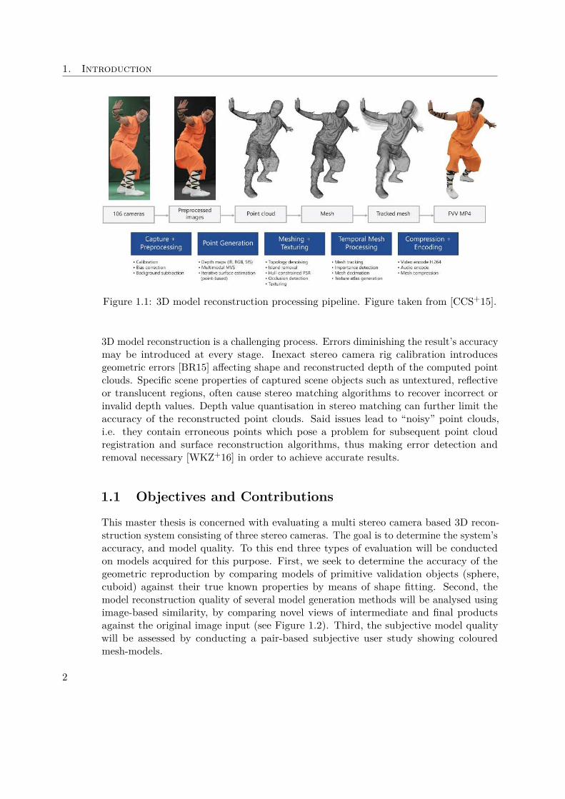
The generation of dynamic 3D model content can be divided into five principal process-ing steps: acquisition and preprocessing, 3D point generation, meshing and texturing,temporal mesh processing and mesh post-processing (see Figure 1.1). A common methodis to capture the scene from multiple view-points with calibrated and registered stereocameras. The resulting image pairs are then used to recover scene depth by means ofstereo matching (e.g. [SNG+15, WFR+16]). The results of matching process are disparitymaps, images whose pixel values encode the scene depth in terms of the horizontaldisplacement between a scene point’s location the input image pairs. Using knowngeometric camera properties, disparity maps can then be turned into 3D point clouds.Surface reconstruction algorithms (e.g. [DTK+16, GG07]) then transfer point clouds intosurface meshes [GG07] or volumetric grids [DTK+16]. In the case of dynamic scenes, thetask of temporary tracking merging models is often performed by non-rigid registration(e.g. [DTK+16]).
1
1. Introduction
Figure 1.1: 3D model reconstruction processing pipeline. Figure taken from [CCS+15].
3D model reconstruction is a challenging process. Errors diminishing the result’s accuracymay be introduced at every stage. Inexact stereo camera rig calibration introducesgeometric errors [BR15] affecting shape and reconstructed depth of the computed pointclouds. Specific scene properties of captured scene objects such as untextured, reflectiveor translucent regions, often cause stereo matching algorithms to recover incorrect orinvalid depth values. Depth value quantisation in stereo matching can further limit theaccuracy of the reconstructed point clouds. Said issues lead to “noisy” point clouds,i.e. they contain erroneous points which pose a problem for subsequent point cloudregistration and surface reconstruction algorithms, thus making error detection andremoval necessary [WKZ+16] in order to achieve accurate results.
1.1 Objectives and Contributions
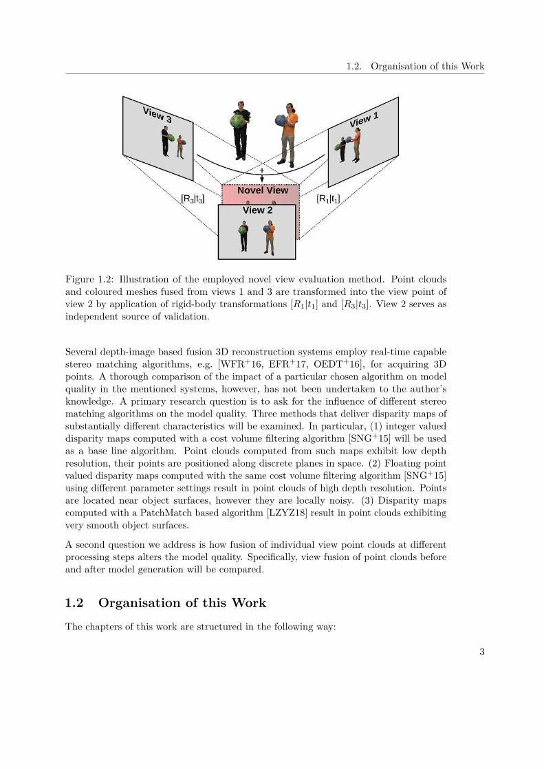
This master thesis is concerned with evaluating a multi stereo camera based 3D recon-struction system consisting of three stereo cameras. The goal is to determine the system’saccuracy, and model quality. To this end three types of evaluation will be conductedon models acquired for this purpose. First, we seek to determine the accuracy of thegeometric reproduction by comparing models of primitive validation objects (sphere,cuboid) against their true known properties by means of shape fitting. Second, themodel reconstruction quality of several model generation methods will be analysed usingimage-based similarity, by comparing novel views of intermediate and final productsagainst the original image input (see Figure 1.2). Third, the subjective model qualitywill be assessed by conducting a pair-based subjective user study showing colouredmesh-models.
2
1.2. Organisation of this Work
Figure 1.2: Illustration of the employed novel view evaluation method. Point cloudsand coloured meshes fused from views 1 and 3 are transformed into the view point ofview 2 by application of rigid-body transformations [R1|t1] and [R3|t3]. View 2 serves asindependent source of validation.
Several depth-image based fusion 3D reconstruction systems employ real-time capablestereo matching algorithms, e.g. [WFR+16, EFR+17, OEDT+16], for acquiring 3Dpoints. A thorough comparison of the impact of a particular chosen algorithm on modelquality in the mentioned systems, however, has not been undertaken to the author’sknowledge. A primary research question is to ask for the influence of different stereomatching algorithms on the model quality. Three methods that deliver disparity maps ofsubstantially different characteristics will be examined. In particular, (1) integer valueddisparity maps computed with a cost volume filtering algorithm [SNG+15] will be usedas a base line algorithm. Point clouds computed from such maps exhibit low depthresolution, their points are positioned along discrete planes in space. (2) Floating pointvalued disparity maps computed with the same cost volume filtering algorithm [SNG+15]using different parameter settings result in point clouds of high depth resolution. Pointsare located near object surfaces, however they are locally noisy. (3) Disparity mapscomputed with a PatchMatch based algorithm [LZYZ18] result in point clouds exhibitingvery smooth object surfaces.
A second question we address is how fusion of individual view point clouds at differentprocessing steps alters the model quality. Specifically, view fusion of point clouds beforeand after model generation will be compared.
1.2 Organisation of this Work
The chapters of this work are structured in the following way:
3
1. Introduction
Chapter 2 introduces selected fundamental concepts of 3D vision used throughout thiswork. First, basic concepts of 3D projective space and 3D transformations will bedescribed. Second, the pinhole camera model will be introduced and extended tothe stereo camera case. Third, the camera calibration procedure is shortly outlined.The chapter focuses on the most important concepts that are used throughout thiswork.
Chapter 3 presents the state-of-the-art in 3D reconstruction of dynamic scenes. First,different methods of depth acquisition hardware and their characteristics sum-marised. Then, fundamental concepts of the employed stereo matching algorithmswill be presented. This includes a summary of popular image similarity measures,stereo matching algorithms, as well different kinds of scene representation. Lastly,model generation algorithms commonly used for reconstruction will be shown.
Chapter 4 presents the state-of-the-art of evaluation methods relevant in this work. Itstarts with an overview of applicable quantitative and qualitative methods. Next,a summary of image-based novel view evaluation follows. Lastly, subjective qualityassessment is explained.
Chapter 5 describes the system under examination and the methods applied for itsevaluation. This chapter comprises two parts. In the first part, the examinedsystem and its processing pipeline are described in detail. Specifically, hardwareand data acquisition, camera calibration and registration, and depth reconstructionwill be discussed. The chapter also contains discussions of failure cases that canarise for each of the described pipeline stages. The chapter’s second part is outlinesthe concrete application of evaluation methods laid out in Chapter 4.
Chapter 6 presents the results of our evaluation. First, the used data set will bepresented, and the approaches we compare will be explained in detail. Second, theresults of the evaluation on validation objects will be shown. Third, the results ofthe novel view evaluation will be presented. Fourth, the results of the user studycarried out within this work will be discussed.
Chapter 7 summarises the covered topics and discusses conclusions that can be drawn.Further, it shows possible future work.
4
CHAPTER 2Fundamentals of 3D
Reconstruction
This chapter recapitulates selected fundamental topics of 3D vision that are employedwithin this work. First, transformations in three-dimensional space are presented. Next,we introduce the pinhole camera, and the stereo camera model, and show how points in3D space are projected onto 2D coordinates of a camera image.
2.1 Transformations in 3D
Intuitively, we can imagine that each object in 3D space has its own coordinate sys-tem attached to it. Transformations formalise the notion of how we can arrive fromthe coordinate frame of one object to that of another. The content in this sectionsummarises selected topics presented in Hartley and Zisserman’s book Multiple ViewGeometry [HZ04].
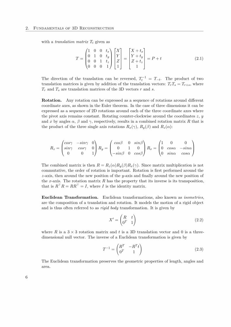
Translation. Translation of an object is presented by shifting it from its attachedcoordinate frame into another coordinate frame that is displaced by the translation vector.Translation can be seen as shifting the origin of object coordinate frame into anotherone given by T = Co − Cc, where T is a three-dimensional vector, Co is the origin of theobject’s original coordinate frame, and Cc is the origin of the object’s new coordinateframe after translation.
A point P = (X, Y, Z) is translated by a vector t = (tx, ty, tz) in homogeneous coordinates
5
2. Fundamentals of 3D Reconstruction
with a translation matrix Tt given as
T =
1 0 0 tx
0 1 0 ty
0 0 1 tz
0 0 0 1
XYZ1
=
X + tx
Y + ty
Z + tz
1
= P + t (2.1)
The direction of the translation can be reversed, T −1t = T−t. The product of two
translation matrices is given by addition of the translation vectors: TrTs = Tr+s, whereTr and Ts are translation matrices of the 3D vectors r and s.
Rotation. Any rotation can be expressed as a sequence of rotations around differentcoordinate axes, as shown in the Euler theorem. In the case of three dimensions it can beexpressed as a sequence of 2D rotations around each of the three coordinate axes wherethe pivot axis remains constant. Rotating counter-clockwise around the coordinates z, yand x by angles α, β and γ, respectively, results in a combined rotation matrix R that isthe product of the three single axis rotations Rx(γ), Ry(β) and Rz(α):
Rz =
cosγ −sinγ 0sinγ cosγ 0
0 0 1
Ry =
cosβ 0 sinβ0 1 0
−sinβ 0 cosβ
Rx =
1 0 00 cosα −sinα0 sinα cosα
The combined matrix is then R = Rz(α)Ry(β)Rx(γ). Since matrix multiplication is notcommutative, the order of rotation is important. Rotation is first performed around thez-axis, then around the new position of the y-axis and finally around the new position ofthe x-axis. The rotation matrix R has the property that its inverse is its transposition,that is R⊤R = RR⊤ = I, where I is the identity matrix.
Euclidean Transformation. Euclidean transformations, also known as isometries,are the composition of a translation and rotation. It models the motion of a rigid objectand is thus often referred to as rigid body transformation. It is given by
X ′ =
(
R t0T 1
)
(2.2)
where R is a 3 × 3 rotation matrix and t is a 3D translation vector and 0 is a three-dimensional null vector. The inverse of a Euclidean transformation is given by
T −1 =
(
RT −RT t0T 1
)
(2.3)
The Euclidean transformation preserves the geometric properties of length, angles andarea.
6
2.2. Camera Models and Calibration
(a) Camera obscura [Zah85]
C optical axisf
P=(X,Y,Z)
p=(x,y,-f)
image plane
X
Y
Z
(b) Pinhole camera model
Figure 2.1: The pinhole camera model.
2.2 Camera Models and Calibration
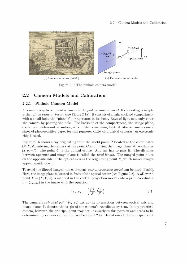
2.2.1 Pinhole Camera Model
A common way to represent a camera is the pinhole camera model. Its operating principleis that of the camera obscura (see Figure 2.1a). It consists of a light enclosed compartmentwith a small hole, the “pinhole”, or aperture, in its front. Rays of light may only enterthe camera by passing the hole. The backside of the compartment, the image plane,contains a photosensitive surface, which detects incoming light. Analogue cameras use asheet of photosensitive paper for this purpose, while with digital cameras, an electronicchip is used.
Figure 2.1b shows a ray originating from the world point P located at the coordinates(X, Y, Z) entering the camera at the point C and hitting the image plane at coordinates(x, y, −f). The point C is the optical centre. Any ray has to pass it. The distancebetween aperture and image plane is called the focal length. The imaged point p lieson the opposite side of the optical axis as the originating point P , which makes imagesappear upside down.
To avoid the flipped images, the equivalent central projection model can be used [Bra00].Here, the image plane is located in front of the optical center (see Figure 2.2). A 3D worldpoint P = (X, Y, Z) is mapped in the central projection model onto a pixel coordinatep = (xu, yu) in the image with the equation
(xu, yu) =(
fX
Z,fY
Z
)
(2.4)
The camera’s principal point (cx, cy) lies at the intersection between optical axis andimage plane. It denotes the origin of the camera’s coordinate system. In any practicalcamera, however, the principal point may not lie exactly at this position and needs to bedetermined by camera calibration (see Section 2.2.4). Deviations of the principal point
7

2. Fundamentals of 3D Reconstruction
Figure 2.2: Frontal projection model. Taken from [Bra00].
from the camera center change the location of mapped image points and needs to becompensated:
(x, y) = (x + cx, y + cy) = (fX
Z+ cx,
fY
Z+ cy) (2.5)
The camera is positioned within the 3D space. To relate the camera’s coordinate systemwith the world coordinate system the following perspective projection is used.
qm⊤ = K[R|t]M⊤ (2.6)
q
uv1
=
fx s cx
0 fy cy
0 0 1
r11 r12 r13 t1
r21 r22 r23 t2
r31 r32 r33 t3
XYZ1
(2.7)
where m⊤ is an image point and M⊤ is a world point. q denotes a scaling factor, fx, fy
are vertical and horizontal focal lengths, cx, cy are the image coordinates of the principal
8

2.2. Camera Models and Calibration
(a) No Distortion (b) Barrel (c) Pincushion (d) Tangential
Figure 2.3: Typical types of lens distortion. A checkerboard pattern (a) when imagedby a camera, exhibits different types of distortion. Barrel distortion (b) and pincushiondistortion (c) are caused by lens manufacturing inaccuracies, whereas tangential dis-tortion (d) is caused by misalignment of the image sensor relative to the image plane.Source: [Bra00]
point and s is the camera’s skew. rij for i, j ∈ 1, 2, 3 is a rotation matrix and t1, t2, t3
is a translation vector.
The matrix K denotes the intrinsic parameters of the camera. It determines the camera’sinternal projection completely and is independent of its position in the world coordinatesystem. The focal length is given both horizontally and vertically and are often assumedto be the same for both directions, fx = fy. This amounts to stating that pixels aresquares. Another common restriction is that the camera does not exhibit skew, that iss = 0.
The joint rotation-translation matrix [R|t] are called extrinsic parameters or its pose. Itrelates the world coordinate system to the camera coordinate system.
2.2.2 Lens Distortion
A physical pinhole camera has significant drawbacks. The small aperture of the pinholelimits the amount of light that can pass onto the image plane in a given time. Further,the focal length is determined by the camera’s physical size. For this reason, practicalcameras use lenses. They allow the adaptation of focal length and correspondingly thefield of view. Moreover, they feature apertures of varying size, which allows controllingthe amount of light that can reach the image plane.
A drawback of using lenses is that they introduce distortion to the images by changingpixel locations of imaged world points. A common way for modelling lens distortionis the Brown-Conrady [Bro66] model. It allows compensating for radial and tangentialdistortion.
Radial Distortion Due to manufacturing inaccuracies, lenses distort the location ofimaged pixels of light rays entering near the lens’ outer rim. Straight lines, for examplethose of a rectangular pattern imaged facing parallel to the image plane (see Figure 2.3a),
9
2. Fundamentals of 3D Reconstruction
become increasingly curved near the image border. This effect is often called barrel orfish-eye distortion (see Figure 2.3b). It is especially noticeable in wide-angle lenses, moreso in those of low quality. The opposite effect, pincushion distortion, bends straight linesinto inwards direction (Figure 2.3c).
The amount of radial distortion is small near the image centre and increases with thedistance from it. It can be modelled in terms of a Taylor series expansion around thecamera’s principle point. Let r be the radius of a circle with the center in the principlepoint, then
xrad = x(1 + k1r2 + k2r4 + k3r6)
yrad = y(1 + k1r2 + k2r4 + k3r6)
where (xrad, yrad) is the image coordinate of the radially distorted pixel and (x, y) is thelocation of the pixel corrected for radial distortion. k1, k2, k3 are the radial distortioncoefficients.
Tangential Distortion Tangential distortion occurs due to the camera’s sensor notbeing aligned parallel with the image plane (Figure 2.3d). It can be characterised asfollows:
xtang = x + [2p1y + p2(r2 + 2x2)]
ytang = y + [p1(r2 + 2y2) + 2p2x]
where (xtang, ytang) is the image coordinate of the radially distorted pixel and (x, y) isthe location of the pixel corrected for tangential distortion. p1, p2 are the tangentialdistortion coefficients.
The tuple of coefficients dist = (k1, k2, p1, p2, k3) determines the combined radial andtangential distortion an imaged pixel. Distortion is independent from image resolutionand only depends on the distance of a pixel from the distortion center, that is assumedto be equal to the camera’s principal point.
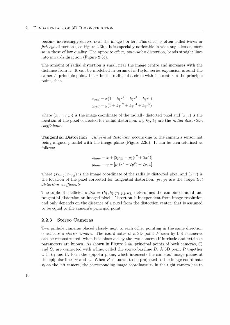
2.2.3 Stereo Cameras
Two pinhole cameras placed closely next to each other pointing in the same directionconstitute a stereo camera. The coordinates of a 3D point P seen by both camerascan be reconstructed, when it is observed by the two cameras if intrinsic and extrinsicparameters are known. As shown in Figure 2.4a, principal points of both cameras, Cl
and Cr are connected with a line, called the stereo baseline B. A 3D point P togetherwith Cl and Cr form the epipolar plane, which intersects the cameras’ image planes atthe epipolar lines el and er. When P is known to be projected to the image coordinatexl on the left camera, the corresponding image coordinate xr in the right camera has to
10
2.2. Camera Models and Calibration
lie on the epipolar line er. If xr it unknown, it is sufficient to restrict the search for it toimage coordinates of er.
The search for an unknown image point xr can be further simplified by virtually movingthe image planes of both cameras in a way that aligns the epipolar lines el and er withhorizontal coordinates of the cameras’ image planes, as shown in Figure 2.4b. Theepipolar lines become parallel to the baseline B. This configuration is said to meet theepipolar constraint. Rectification of a stereo camera involves modifying both cameras’relative pose (R, t) so that the epipolar constraint is met. Determining suitable relativeposes of both views of a stereo camera is a task of stereo camera calibration. If theepipolar constraint is met, the search for an unknown corresponding image point xr fora known image point xl reduces to a one dimensional scan for x coordinate at the ycoordinate of xl in the right camera’s image plane. The difference between xl and xr
is called the disparity d of point P . With known point correspondences xl and xr, thedistance of P to the stereo camera can be determined by the method of similar triangles(see Figure 2.4c), resulting in the following formula for the distance Z of point P
Z =f ∗ B
xl − xr=
f ∗ B
d(2.8)
where f is the camera’s focal length in pixels. B is the base line in meters. xl and xr
denote horizontal pixel coordinates in the left and right camera image, respectively. Theirdifference is the disparity denoted by d.
2.2.4 Stereo Camera Calibration
Camera calibration refers to determining the intrinsic and extrinsic camera parameters.When these are known, 3D world points can be projected to 2D image coordinates andvice versa. Calibration involves acquiring images of objects with well-known dimensions.Camera parameters are then determined by relating object properties with their imagedcounterparts.
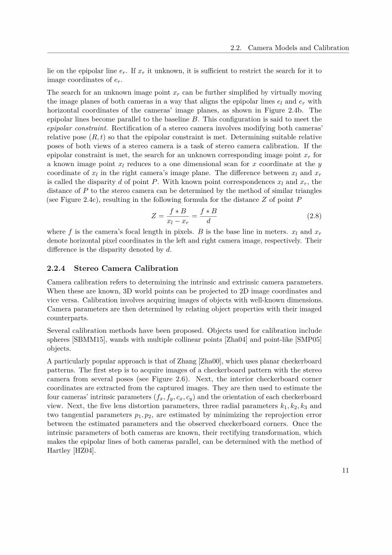
Several calibration methods have been proposed. Objects used for calibration includespheres [SBMM15], wands with multiple collinear points [Zha04] and point-like [SMP05]objects.
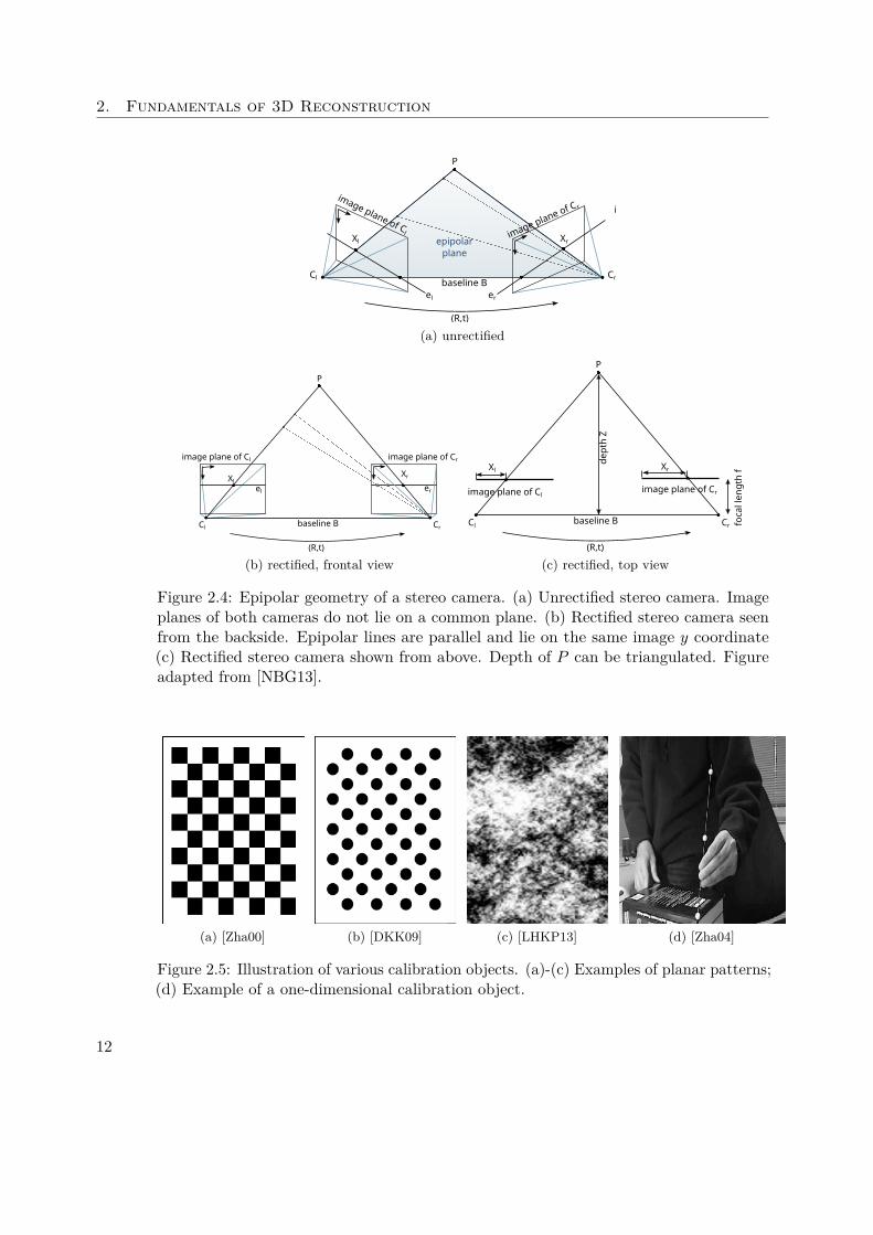
A particularly popular approach is that of Zhang [Zha00], which uses planar checkerboardpatterns. The first step is to acquire images of a checkerboard pattern with the stereocamera from several poses (see Figure 2.6). Next, the interior checkerboard cornercoordinates are extracted from the captured images. They are then used to estimate thefour cameras’ intrinsic parameters (fx, fy, cx, cy) and the orientation of each checkerboardview. Next, the five lens distortion parameters, three radial parameters k1, k2, k3 andtwo tangential parameters p1, p2, are estimated by minimizing the reprojection errorbetween the estimated parameters and the observed checkerboard corners. Once theintrinsic parameters of both cameras are known, their rectifying transformation, whichmakes the epipolar lines of both cameras parallel, can be determined with the method ofHartley [HZ04].
11
2. Fundamentals of 3D Reconstruction
baseline BCl Cr
P
image plane of Cl
epipolarplane
image plane of C r
Xl Xr
(R,t)
el er
i
(a) unrectified
image plane of Cr
P
Cl Cr
image plane of Cl
Xl
(R,t)
el er
Xr
baseline B
(b) rectified, frontal view
Cl Cr
image plane of Cl
baseline B
Xl
(R,t)
image plane of Cr
Xr
foca
l le
ng
th f
de
pth
Z
P
(c) rectified, top view
Figure 2.4: Epipolar geometry of a stereo camera. (a) Unrectified stereo camera. Imageplanes of both cameras do not lie on a common plane. (b) Rectified stereo camera seenfrom the backside. Epipolar lines are parallel and lie on the same image y coordinate(c) Rectified stereo camera shown from above. Depth of P can be triangulated. Figureadapted from [NBG13].
(a) [Zha00] (b) [DKK09] (c) [LHKP13] (d) [Zha04]
Figure 2.5: Illustration of various calibration objects. (a)-(c) Examples of planar patterns;(d) Example of a one-dimensional calibration object.
12
2.2. Camera Models and Calibration
Figure 2.6: Camera calibration with planar patterns. Figure taken from [BKB08].
13

CHAPTER 33D Reconstruction Using
Multiple Depth Sensors
In this chapter, we present the state-of-the-art related to our approach to 3D reconstruc-tion that is suited for acquiring dynamic scenes in a controlled environment. Here, depthsensors are positioned statically around an acquisition area. Each sensor acquires 3Dinformation from its own viewpoint. Individual views of the scene are then fused tocombined 3D models.
This chapter is structured as follows. In Section 3.1, we give an overview of employed dataacquisition techniques. Next, we discuss how depth information can be reconstructedfrom image pairs in Section 3.2. Lastly, the fusion of views into combined models areexplained in Section 3.3.
3.1 Data Acquisition
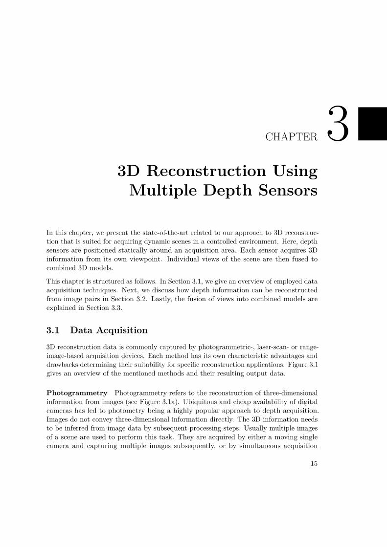
3D reconstruction data is commonly captured by photogrammetric-, laser-scan- or range-image-based acquisition devices. Each method has its own characteristic advantages anddrawbacks determining their suitability for specific reconstruction applications. Figure 3.1gives an overview of the mentioned methods and their resulting output data.
Photogrammetry Photogrammetry refers to the reconstruction of three-dimensionalinformation from images (see Figure 3.1a). Ubiquitous and cheap availability of digitalcameras has led to photometry being a highly popular approach to depth acquisition.Images do not convey three-dimensional information directly. The 3D information needsto be inferred from image data by subsequent processing steps. Usually multiple imagesof a scene are used to perform this task. They are acquired by either a moving singlecamera and capturing multiple images subsequently, or by simultaneous acquisition
15
3. 3D Reconstruction Using Multiple Depth Sensors
Figure 3.1: Data acquisition methods and their results. (a) Photogrammetric acquisitionyields RGB images. Source: [Nym17]; (b) Laser scanning devices produce uncolouredpoint clouds, illustrated as colour-mapped. Source: [Mon07]; (c) Time-of-flight camerasmay produce RGB-D images. Source: [EA14].
with multiple cameras at different positions. Depth information can then be recoveredby identifying corresponding image points and triangulating them between multipleimages (see Section 2.2.3). Although this way of depth acquisition is prone to errorsand requires a significant amount of computation, it is also the most flexible depthreconstruction method. Applications of photogrammetry range from highly precise depthmeasurements of small objects [BKH10, SCD+06], over large-scale reconstruction ofterrain [ZTDVAL14] and urban areas [LNSW16] to the acquisition of highly dynamicscenes [DTK+16, EFR+17, CCS+15].
Range Images Range imaging is an active method of depth acquisition. A signalcreated by the depth sensor interacts with the scene and is then measured by the sensor.Two predominant technologies delivering range images are structured-light [HLCH12,SLK15] and time-of-flight (TOF) [HLCH12, SAB+07]. Figure 3.1c illustrates the popularKinect One sensor and an acquired point cloud that exhibits depth as well as RGB colourinformation (i.e. RGB-D). In structured light techniques, a pattern is projected onto ascene, usually in the near infra-red spectrum invisible to the human eye. The pattern isdistorted by the scene and is again captured by a monochrome charge-coupled-device(CCD) image sensor. Examples of recent high performance real-time 3D acquisitionsystems employing structured light are e.g. [DTK+16, OEDT+16]. There, additionalRGB cameras are used to acquire colour information for model texturing. TOF cameras,on the other hand, achieve similar results by measuring runtime differences of light sentby the sensor and reflected by scene objects. Range image cameras are able to provide
16

3.2. Depth Reconstruction
depth maps and colour images simultaneously. The spatial resolution of depth maps isusually limited, as is the maximal achievable measurement distance. The popular KinectOne sensor has a depth image resolution of 512 × 424 pixels and can measure distancesof up to 4.5 meters with a frame rate of up to 30 Hz [SLK15].
3.2 Depth Reconstruction
We will now discuss how 3D models can be recovered from images of a scene. We start bypresenting image-based measures that can be used to find corresponding regions amongmultiple images. Next, depth reconstruction from stereo image pairs is elaborated. Lastly,common ways of scene representation are explained.
3.2.1 Image Similarity
A key task for any reconstruction algorithm is to identify corresponding points or featureswithin two or more images. Image similarity, also called photo-consistency, captures thisconcept. An object’s illumination and colour can change significantly when viewed fromdifferent positions due to directional light sources, or object material. It is desirable forsimilarity measures to be invariant to such changes.
We can distinguish sparse and dense approaches. In the first category, we have featuredescriptors (e.g. SIFT [Low04] or SURF [BTV06]) that identify prominent image regions.They are considered sparse, as they only track prominent image regions, such as edgesor contours. The second are dense similarity functions that assign a numerical value toevery pixel of an image. Given a set of N images and a 3D point p seen in every , we candefine photo-consistency [FH15] between pairs of images Ii and Ij , i, j ∈ (1, . . . , N) as
Cij(p) = ρ(Ii(Ω(πi(p))), Ij(Ω(πj(p)))), (3.1)
where ρ is a similarity function, πi(p) is the projection that maps the 3D point p intoimage i, Ω(x) defines a support region, also called domain, around point p and Ii(x)denotes the intensity or colour values of pixels within the domain. The choice of ρ andΩ describes a particular similarity measure. Note that image coordinates are integral,whereas πi(p) is real valued. To accommodate 3D points that are projected onto real-valued coordinates some interpolation scheme is needed. Further, the described similaritymeasures operate on single channel images only. RGB images require preprocessing inorder to determine similarity. One way is to perform computation on grey-scale versions.Another way is to compute similarity on each of the three colour channels separately,and then combine the results by pixel-wise averaging [FH15].
We give details on three commonly used similarity measures.
• Sum of Absolute Differences (SAD) is defined as the L1 norm between twovectors of pixel intensity values in support regions f and g around the image
17
3. 3D Reconstruction Using Multiple Depth Sensors
coordinates to which a 3D point p is projected. More formally,
ρSAD(f, g) = ||f − g||1 (3.2)
SAD is sensitive to brightness and contrast changes. It is useful mainly for imagesof similar illumination characteristics. On the other hand, SAD is computationallycheap, which makes it useful for real-time applications that can guarantee similarimage illumination.
• Normalised Cross Correlation (NCC). The normalised cross coefficient is anestablished tool for determining image similarity in presence of illumination andexposure changes. It is a statistical measure defined as
ρNCC(f, g) =(f − f) · (g − g)
σf σg∈ [−1, 1] (3.3)
where f , g denote the mean values and σf and σg the standard deviations of pixelintensity values within the domains around the pixels projected into Ii and Ij ,respectively.
Its invariance to illumination changes makes NCC one of the most commonly usedsimilarity measures in two-view and multi-view stereo. NCC, however, fails todetect pixels in untextured regions.
• Census [ZW94] Census is one of the best performing similarity measures for stereocorrespondences [HS07]. In contrast to other presented measures, it does not useintensity values themselves, but first computes a bit string describing whetherpixels within the support domain of a pixel p are lighter or darker than p and thencomputes the Hamming distance between the two resulting bit strings.
Formally, a comparison operator is defined that determines whether a pixel a isbrighter than a pixel b
ξ(a, b) = 1 if a < b, 0 otherwise, (3.4)
A bit string describing brighter and darker pixels in Ω is computed as
census(f) = ⊕q∈Ωξ(f(p), f(q)), (3.5)
where ⊕ is the concatenation operator and p and q are image pixels. The Censusscore is then the Hamming distance of the two bit strings.
ρCensus(f, g) = |census(f) − census(g)|1 ∈ [0, N ] (3.6)
where N is the size of the support region Ω. Census is especially robust againstimage brightness and contrast changes, as well as around depth boundaries.
18
3.2. Depth Reconstruction
3.2.2 Stereo Matching
Stereo matching is the problem of recovering depth from image pairs that are slightlydisplaced akin to human eyes (see Figure 3.2a). After appropriate rectification, theimaged objects exhibit a horizontal displacement, called disparity, depending on theirdistance to the camera. It is measured in terms of the number of displaced pixels. Nearobjects have high disparity, whereas objects that are more distant have low disparity.For example, the chimney edge shown in Figure 3.2 appears in the left view at pointPl and in the right view as Pr. The disparity between these points is denoted as dP .The Teddy’s ear, on the other hand, is marked as Ql and Qr respectively, and is locatedfurther in the backside of the scene. The chimney is nearer than the ear, and we havedP > dQ. A stereo matching algorithm computes depth in form of a disparity map, whichis a single channel image whose pixel intensity values correspond to the scene disparityat pixels in the corresponding (left) input image.
Assumptions. Stereo matching algorithms commonly make some assumptions tocompute disparity maps. The first one is the photo consistency assumption. It demandsthat corresponding pixels in the left and right view have the same colour values. Next,there is the epipolar assumption, requiring that corresponding pixels in left and right viewalways appear on a horizontal line. This is ensured by image rectification explained inSection 2.2.3. The smoothness assumption states that spatially close pixels have similardisparity values. The smoothness assumption holds in most image regions, except forobject borders.
Types of Stereo Matching Algorithms. Stereo Matching algorithms can be broadlycategorised by the way they determine point correspondences. Local methods finddisparity values by searching for each pixel in the left view a corresponding pixel in theright view by sliding local windows along horizontal image lines. A typical example forlocal stereo matching is the cost volume filtering technique [HRB+13, SNG+15]. Globalmethods minimise an explicit energy function over all image pixels. A typical energyfunction [BB13] has the form
E(p) = Edata(p) + λEsmooth(p)
where E(p) is the total energy value of an image pixel p. The data term Edata accounts forcolour similarity. Esmooth, the smoothness term, captures local object smoothness. Theparameter λ ∈ R balances is the relative influence of the terms Edata and Esmooth. Com-mon examples for global stereo matching algorithms are dynamic programming [BT99]and belief propagation [FH06]. An elaborate discussion on global stereo methods can befound in [BB13].
Learning based methods rely on machine learning methods for depth estimation. There,first a model is trained with ground truth data, and then the trained model can beused to estimate depth. An example for a learning based algorithm is the Global PatchCollider [WFR+16]. It uses random forests to represent the model.
19

3. 3D Reconstruction Using Multiple Depth Sensors
(a) Left and Right View (b) Disparities (c) Disparity Map
Figure 3.2: Stereo matching. (a) Left input view (top), right input view (bottom). (b)Disparity dP of a nearer object, marked as Pl and Pr in left and right input is large,while objects father away, e.g. Ql, and Qr, exhibit a lower displacement dQ. (c) Disparitymap: intensities encode the disparity value.
Stereo Matching Pipeline. Stereo matching algorithms generally have to perform thesame processing steps [SS02], regardless whether they are local or global algorithms. Inthe following, the conceptual processing steps involved are summarised. Specific methodsmay skip or aggregate some steps. As the 3D reconstruction system addressed in thiswork employs primarily a local stereo matching algorithm, the focus lies on local methods.Local algorithms compute disparity by searching for each pixel potentially matchingcandidates in the other image in a pre-defined search range (Figure 3.3b). The completesearch space is often called Disparity Space Image [SS02], or cost volume [BRR11].Candidate search can be limited to pixels on the same horizontal line when relying onrectified input images (Figure 3.3a).
Cost Computation (CC). Pixels are compared using some dissimilarity- or cost-measure that takes into account a small support region around pixels. Measures thatare typically employed include SAD, NCC or Census. They have been discussed inSection 3.2.1.
Cost Aggregation (CA). Local methods usually enforce spatial consistency im-plicitly in the Cost Aggregation stage (Figure 3.3c). This process can be viewed asfiltering of the cost volume [HRB+13]. Cost aggregation has a significant impact
20
3.2. Depth Reconstruction
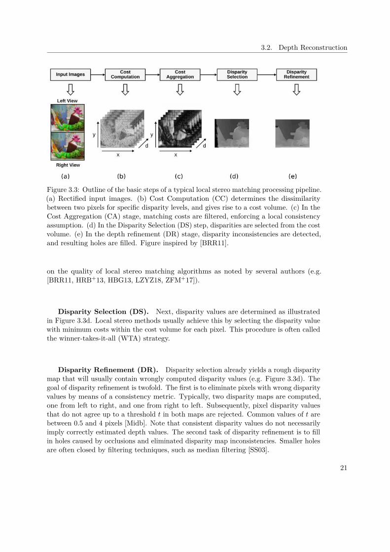
Figure 3.3: Outline of the basic steps of a typical local stereo matching processing pipeline.(a) Rectified input images. (b) Cost Computation (CC) determines the dissimilaritybetween two pixels for specific disparity levels, and gives rise to a cost volume. (c) In theCost Aggregation (CA) stage, matching costs are filtered, enforcing a local consistencyassumption. (d) In the Disparity Selection (DS) step, disparities are selected from the costvolume. (e) In the depth refinement (DR) stage, disparity inconsistencies are detected,and resulting holes are filled. Figure inspired by [BRR11].
on the quality of local stereo matching algorithms as noted by several authors (e.g.[BRR11, HRB+13, HBG13, LZYZ18, ZFM+17]).
Disparity Selection (DS). Next, disparity values are determined as illustratedin Figure 3.3d. Local stereo methods usually achieve this by selecting the disparity valuewith minimum costs within the cost volume for each pixel. This procedure is often calledthe winner-takes-it-all (WTA) strategy.
Disparity Refinement (DR). Disparity selection already yields a rough disparitymap that will usually contain wrongly computed disparity values (e.g. Figure 3.3d). Thegoal of disparity refinement is twofold. The first is to eliminate pixels with wrong disparityvalues by means of a consistency metric. Typically, two disparity maps are computed,one from left to right, and one from right to left. Subsequently, pixel disparity valuesthat do not agree up to a threshold t in both maps are rejected. Common values of t arebetween 0.5 and 4 pixels [Midb]. Note that consistent disparity values do not necessarilyimply correctly estimated depth values. The second task of disparity refinement is to fillin holes caused by occlusions and eliminated disparity map inconsistencies. Smaller holesare often closed by filtering techniques, such as median filtering [SS03].
21
3. 3D Reconstruction Using Multiple Depth Sensors
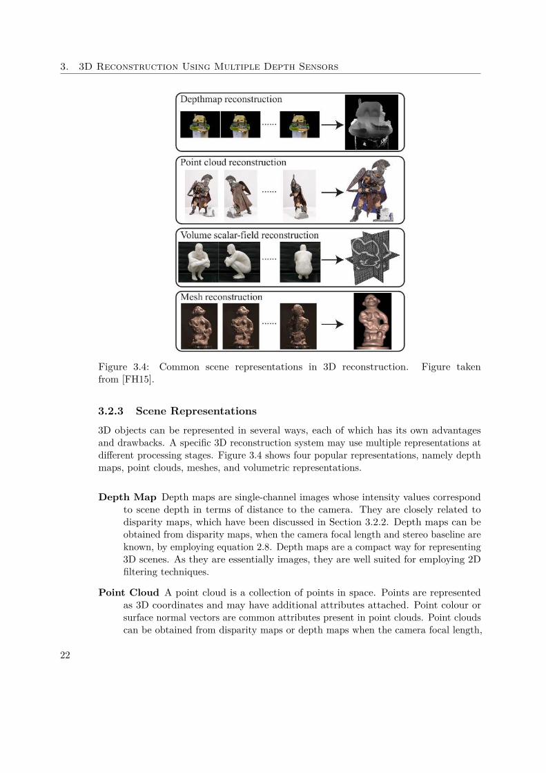
Figure 3.4: Common scene representations in 3D reconstruction. Figure takenfrom [FH15].
3.2.3 Scene Representations
3D objects can be represented in several ways, each of which has its own advantagesand drawbacks. A specific 3D reconstruction system may use multiple representations atdifferent processing stages. Figure 3.4 shows four popular representations, namely depthmaps, point clouds, meshes, and volumetric representations.
Depth Map Depth maps are single-channel images whose intensity values correspondto scene depth in terms of distance to the camera. They are closely related todisparity maps, which have been discussed in Section 3.2.2. Depth maps can beobtained from disparity maps, when the camera focal length and stereo baseline areknown, by employing equation 2.8. Depth maps are a compact way for representing3D scenes. As they are essentially images, they are well suited for employing 2Dfiltering techniques.
Point Cloud A point cloud is a collection of points in space. Points are representedas 3D coordinates and may have additional attributes attached. Point colour orsurface normal vectors are common attributes present in point clouds. Point cloudscan be obtained from disparity maps or depth maps when the camera focal length,
22
3.3. View Fusion
principal point and stereo baseline are known, as shown in Section 2.2.1. Depthmaps, in result, are often treated as geometric proxy for point clouds.
Polygon Mesh Meshes, specifically polygonal, 3D meshes, are collections of vertices,edges and faces. Vertices correspond to points of a 3D point cloud. Edges define(typically triangular) faces attached to mesh vertices, and approximate an object’ssurface. Algorithms commonly used to reconstruct meshes from point cloudsare the Screened Poisson surface reconstruction [KH13], and Algebraic Point SetSurfaces [GG07].
Volumetric Representations Volumetric representations were originally proposedin [CL96] for range images. Here, the scene space is divided into a three-dimensionalregular grid of cells, also called voxels (e.g. volumetric pixels). Each voxel storesthe value of a signed distance function (SDF) that describes the distance of avoxel’s center to an object’s surface. Voxels also have a weight that accounts forthe measurement reliability. Positive SDF values denote voxels in front of a surfacepoint p. Voxels behind p have negative values. Often, the SDF is truncated (TSDF)to some threshold ±t to allow a compact representation of small distances. Anobject’s surface is implicitly represented within the volume by the TSDF’s zerocrossings. The potential accuracy of regular voxel grids is determined by volumesize and grid resolution. A high memory demand of Θ(n3) complexity in the gridsize n, makes them impractical for precise real-time applications. Hierarchicalvolumetric grids lower the memory consumption by storing voxels in an octree-likedata structure that provides high spatial resolution only for regions containing closepoints (e.g. [DTK+16]). Volumetric representations are popular in 3D reconstructionsystems for dynamic scenes (e.g [DTK+16, OEDT+16, YGX+17, CCS+15]) becausethey are well suited for spatial fusion of multiple views, as well as temporal fusionof subsequent sensor readings.
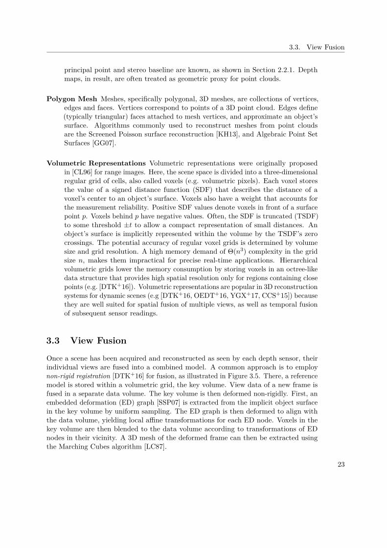
3.3 View Fusion
Once a scene has been acquired and reconstructed as seen by each depth sensor, theirindividual views are fused into a combined model. A common approach is to employnon-rigid registration [DTK+16] for fusion, as illustrated in Figure 3.5. There, a referencemodel is stored within a volumetric grid, the key volume. View data of a new frame isfused in a separate data volume. The key volume is then deformed non-rigidly. First, anembedded deformation (ED) graph [SSP07] is extracted from the implicit object surfacein the key volume by uniform sampling. The ED graph is then deformed to align withthe data volume, yielding local affine transformations for each ED node. Voxels in thekey volume are then blended to the data volume according to transformations of EDnodes in their vicinity. A 3D mesh of the deformed frame can then be extracted usingthe Marching Cubes algorithm [LC87].
23
3. 3D Reconstruction Using Multiple Depth Sensors
Figure 3.5: View fusion with non-rigid alignment. Figure taken from [DTK+16].
3.4 Summary
In this chapter, we have presented the principles and state of the art of 3D reconstructionusing multiple sensors. The processing pipeline acquires dynamic 3D models fromstatically positioned stereo cameras, and computes point clouds with stereo matching.Point clouds of individual viewpoints are fused into a combined object model from whichpolygonal meshes are extracted. We have presented the two main methods of acquiringscene data, namely photogrammetry and range imaging. Further, we have discussed howscene depth is computed from stereo camera images by means of stereo matching. Lastly,we have outlined how 3D models from single views are combined into 3D mesh modelswith non-rigid registration.
24

CHAPTER 4Evaluation Methods
This chapter introduces the state-of-the-art methods for evaluation 3D reconstructionsystem.
The following chapter is structured as follows. Section 4.1 provides an overview ofavailable evaluation methods. Next, Section 4.2 focuses on image-based novel viewevaluation. Finally, Section 4.3 discusses subjective evaluation in more detail.
4.1 Overview of Evaluation Methods
3D reconstruction systems can be evaluated in several ways. Figure 4.1 provides anoverview. In particular, we can distinguish between quantitative and qualitative evalua-tion. Quantitative evaluation analyses properties of observations numerically. Qualitativeevaluation, on the other hand, is concerned with comparing the subjective impression ofan observation or product. Here, we focus on quantitative methods, while Section 4.3 isconcerned with qualitative subjective evaluation.
Quantitative evaluation can further be categorised into methods that are ground truthbased and those without ground truth. An overview of 3D visual content datasets in thecontext of 3D video quality evaluation can be found in [FBC+18].
Ground Truth-based Methods. In the context of 3D reconstruction, ground truth isdata set containing highly accurate reference solutions, such as disparity maps [Midb] orpoint cloud [SSG+17]. Creation of ground truth data sets (e.g. [Mida, Midb, KIT]) for 3Dreconstruction is often performed with structured light [SS02, SS03, SHK+14, SCD+06]or laser scanners [GLU12, SSG+17]. Given a ground truth data set, the deviation ofthe result of a compared method can be determined using an error measure. A typicalmeasure often employed in the field of stereo matching is the Bad Matched Pixel (BMP)error (e.g. [CTF12]). It is defined as the ratio of disparity map pixels, whose values
25

4. Evaluation Methods
Ground Truth based Without Ground Truth
Quantitative Methods Qualitative Methods
Non-dense
Histogram based
ROC based
Error Measure
Disparity Quality
Prediction Error
Confidence Measures
Evaluation Methods
Subjective Evaluation
Using two Views
Using three Views
Shape fitting based
Paired Comparison
Absolute Rating
Figure 4.1: Taxonomy of evaluation methods. Figure adapted from [VCB15]
deviate from a ground truth disparity map more than a threshold value. BMP is definedover every valid pixel and is said to be dense. In contrast, non-dense methods, such ashistogram- or Receiver Operator Characteristic (ROC), measure ground truth deviationsonly for certain regions of the ground truth. Further, shape-fitting relies on the measuringfeatures of reconstructed models and comparing them with real-world counter parts, suchas edge lengths of a complex manufactured product [BKH10].
Methods without Ground Truth. In cases where no direct comparison to groundtruth data is available or viable, sources of validation can be obtained directly from theinput data. This approach can be distinguished into two categories, confidence basedand prediction error based methods. Confidence-measures can be computed from thereconstruction input alone. High confidence values correlate with high reconstructionquality. An example for a confidence measure in stereo vision is the Left-Right consistencycheck that is computed from two corresponding disparity maps. Numerous other measureshave been proposed (e.g. [HM12]). Prediction error-based evaluation methods are image-based methods that employ image warping to align input data to the reconstruction output.One way, often seen in stereo vision, is to acquire data with a third camera and to use theadditional sensor data as source of validation [Sze99, CGK14, MK09, SCSK13, SCK15].Another way, which is often used in image-based rendering, is to directly employ inputimages for validation [WBF+17, VV14]. Both methods will be discussed in the followingSection 4.2.
26
4.2. Image-based Novel View Evaluation
4.2 Image-based Novel View Evaluation
Image-based novel view methods allow evaluating a 3D reconstruction system in absenceof ground truth data provided by a ready-made data set, or a high-precision depthsensor, such as a measurement laser. They validate against an image that is acquired orcomputed in the course of the acquisition process. We can distinguish methods that relyon an additional sensor, and those that do not.
4.2.1 Third-Eye Technique
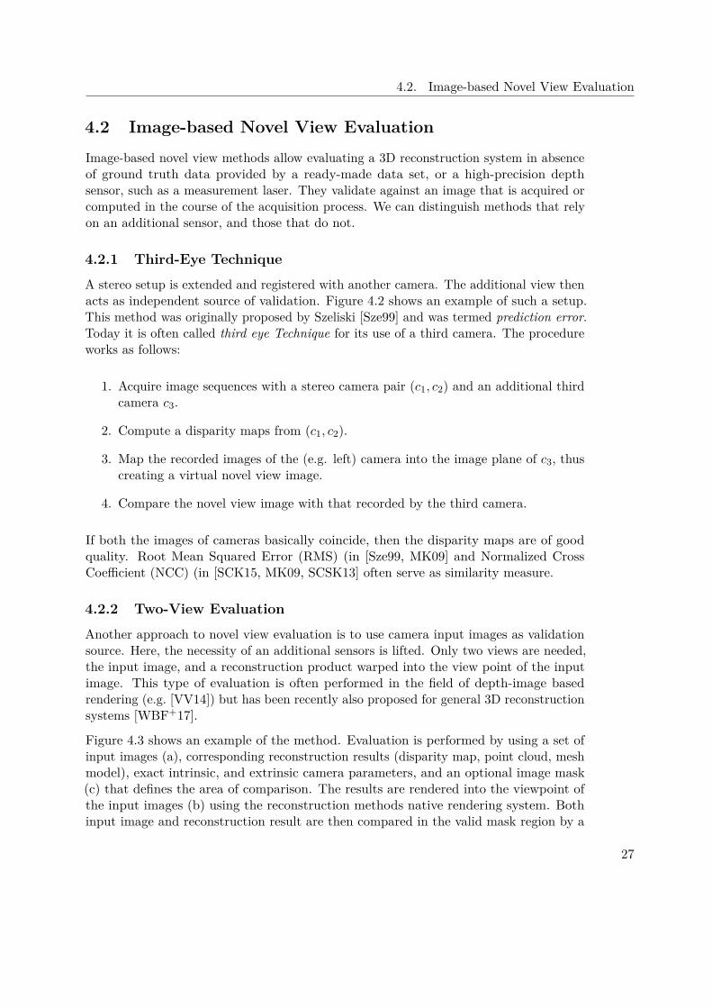
A stereo setup is extended and registered with another camera. The additional view thenacts as independent source of validation. Figure 4.2 shows an example of such a setup.This method was originally proposed by Szeliski [Sze99] and was termed prediction error.Today it is often called third eye Technique for its use of a third camera. The procedureworks as follows:
1. Acquire image sequences with a stereo camera pair (c1, c2) and an additional thirdcamera c3.
2. Compute a disparity maps from (c1, c2).
3. Map the recorded images of the (e.g. left) camera into the image plane of c3, thuscreating a virtual novel view image.
4. Compare the novel view image with that recorded by the third camera.
If both the images of cameras basically coincide, then the disparity maps are of goodquality. Root Mean Squared Error (RMS) (in [Sze99, MK09] and Normalized CrossCoefficient (NCC) (in [SCK15, MK09, SCSK13] often serve as similarity measure.
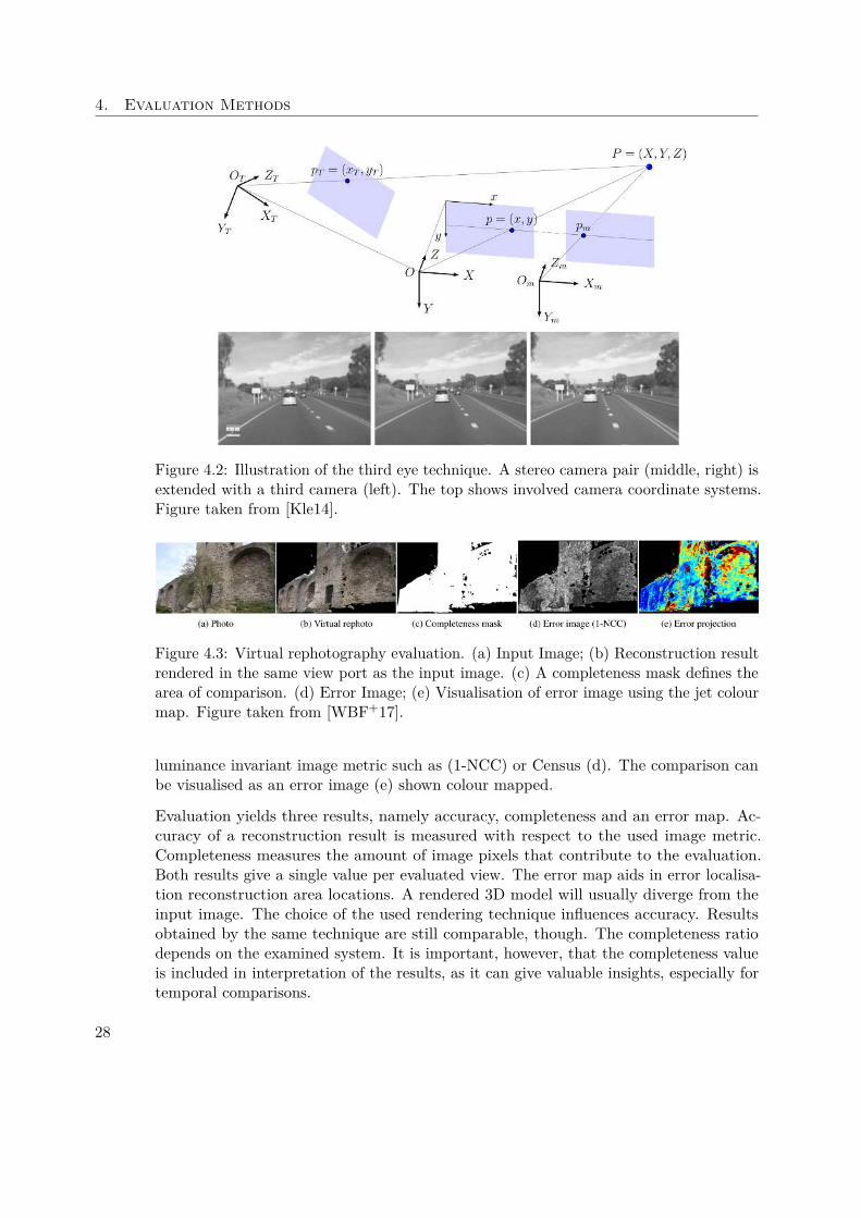
4.2.2 Two-View Evaluation
Another approach to novel view evaluation is to use camera input images as validationsource. Here, the necessity of an additional sensors is lifted. Only two views are needed,the input image, and a reconstruction product warped into the view point of the inputimage. This type of evaluation is often performed in the field of depth-image basedrendering (e.g. [VV14]) but has been recently also proposed for general 3D reconstructionsystems [WBF+17].
Figure 4.3 shows an example of the method. Evaluation is performed by using a set ofinput images (a), corresponding reconstruction results (disparity map, point cloud, meshmodel), exact intrinsic, and extrinsic camera parameters, and an optional image mask(c) that defines the area of comparison. The results are rendered into the viewpoint ofthe input images (b) using the reconstruction methods native rendering system. Bothinput image and reconstruction result are then compared in the valid mask region by a
27
4. Evaluation Methods
Figure 4.2: Illustration of the third eye technique. A stereo camera pair (middle, right) isextended with a third camera (left). The top shows involved camera coordinate systems.Figure taken from [Kle14].
Figure 4.3: Virtual rephotography evaluation. (a) Input Image; (b) Reconstruction resultrendered in the same view port as the input image. (c) A completeness mask defines thearea of comparison. (d) Error Image; (e) Visualisation of error image using the jet colourmap. Figure taken from [WBF+17].
luminance invariant image metric such as (1-NCC) or Census (d). The comparison canbe visualised as an error image (e) shown colour mapped.
Evaluation yields three results, namely accuracy, completeness and an error map. Ac-curacy of a reconstruction result is measured with respect to the used image metric.Completeness measures the amount of image pixels that contribute to the evaluation.Both results give a single value per evaluated view. The error map aids in error localisa-tion reconstruction area locations. A rendered 3D model will usually diverge from theinput image. The choice of the used rendering technique influences accuracy. Resultsobtained by the same technique are still comparable, though. The completeness ratiodepends on the examined system. It is important, however, that the completeness valueis included in interpretation of the results, as it can give valuable insights, especially fortemporal comparisons.
28

4.3. Subjective Quality Assessment
4.3 Subjective Quality Assessment
The quality of 3D point clouds and meshes can be determined by means of subjectivequality assessment. Here, the observer’s perception constitutes a ground truth value.The International Telecommunication Union (ITU) has published recommendations onhow to conduct subjective quality assessment in the context of television system. Theaim is to arrive at meaningful, unbiased and reproducible evaluation results. A thoroughreview of different methods for measuring the quality of experience related to 3D videocontent can be found in [BÁBB+18]
This section is structured as follows. We start by introducing state-of-the-art in subjectiveassessment of 3D meshes and specific considerations when doing so in Section 4.3.1.Then, we continue by elaborating on study design and procedures to conduct subjectiveassessments in Section 4.3.2. Finally, commonly applied testing methodologies arediscussed in Section 4.3.2.
4.3.1 Subjective Assessment of 3D Models
Subjective assessment of mesh models is often performed to determine the influence ofalgorithms modifying them, such as compression [GVC+16] and watermarking [CGEB07].Another area is performance testing of quality measures [VSKL17, AUE17, TWC15].Traditionally these studies use high quality benchmark data sets such as [SCD+06].Subjective evaluation of dynamically captured 3D models, on the other hand, is anarea of active research. Only few publications are concerned with quality assessment ofdynamic [TWC15], or captured mesh models [DZC+18].
For subjective assessment of 3D models, no specific recommendation has been proposedby ITU, so authors usually adopt one of the test procedures of ITU BT-500.13 [ITU12]or ITU P.910 [ITU08]. These recommendations target evaluation of images, and videosin the context of television systems. Contrary to images and videos, point clouds andmesh models allow an observer to regard them from multiple viewpoints. Fixed viewinteraction just shows one preselected view [TWC15]. Free view interaction allows theobserver to view the test material by his choice. This includes free rotation, translationand zooming. [TWC15] This procedure has two shortcomings. The first is cognitiveoverload of the observer. The other issue is, that each observer will have a differentimpression of the test material, which can bias assessment results. Another approach touser interaction is adopted in [GVC+16], where animated renderings of the material isshown. This hybrid technique allows observers to regard the material from multiple viewpoints, while guaranteeing reproducible impressions. Torkhani et. al [TWC15] observe asignificant difference between mean objective scores given by viewers of free view andfixed view setting.
Additional factors to consider when assessing quality of 3D models are the type of shadingmethod and scene illumination. Guo et.al [GVC+16] notes that choice of position andtype of illumination has as strong impact on the observer’s perception of mesh models.
29

4. Evaluation Methods
Characteristic Condition
Maximum observation angle 30 degRatio of luminance background behind picture monitor to peak pictureluminance
≈ 0.15
Background Chromacity D65Room illumination low
Table 4.1: Viewing conditions for subjective assessment as defined in ITU Recommenda-tion ITU-R BT.500 [ITU12]
Corsini et. al suggest the use of a non-uniform background [CGEB07] and extensivelycomment on rendering conditions.
4.3.2 Study Design and Environmental Conditions
Extensive recommendations exist concerning the testing environment and the studydesign.
Environment. To ensure meaningful results, ITU recommends a controlled environ-ment in which study participants perform their task. Table 4.1 summarises the mostimportant aspects of a suitable environment. Observers should be seated in a distraction-free room of neutral colour and low light conditions. They should sit orthogonally to theevaluation screen.
Study Design. At least fifteen observers are recommended [ITU08]. For preliminarystudies, 4 to 8 persons are sufficient. It is important to report supplemental informationon the observers in order to be able to put observations into context. Particulars toreport are, for example, whether the observers are naïve (non-experts) or experts, theirlevel of expertise, occupation category (student, professor), as well as gender and agerange. It is advised to include as much detail as possible in the assessment. A trial startswith observers being introduced to the task. Next, they need to be screened for visualacuity to ensure they are able to make sensible judgements. A training phase makessure participants have understood the task at hand. Then, a testing phase starts, toallow observers to familiarise themselves with the task. Test sessions are expected tolast up to 30 minutes, to avoid subject exhaustion. The exact mode and sequence ofshown material depends on the goals of the study. A number of testing methodologiesoften used for 3D mesh model evaluation is discussed in Section 4.3.3. For image content,the recommended show time of a single stimulus is approximately 4 seconds. Dynamiccontent, such as video needs to be presented for a longer time, approximately 10 seconds,these times can be adapted in a particular study.
30
4.3. Subjective Quality Assessment
4.3.3 Testing Methodologies
In order to meet the needs of varying assessment purposes and contexts a numberof testing protocols have been proposed. Two broad categories can be distinguished,impairment and quality. Impairment protocols assume comparison of a degraded, orsomehow altered test signal against a references signal of known characteristics. Qualityprotocols, on the other hand, assess quality of either a single or multiple stimuli.
• Absolute categorical rating (ACR) [ITU08] is also called single stimulus method.It is especially useful, to assess quality in absence of a reference signal. One stimulusis presented at a time, after that observers judge on a five grade scale.
• Double-Stimulus continuous quality-scale (DSQS) [ITU12] is appropriate ifa new system tested, or impairment parameters cannot be varied. Observersare shown a series of picture pairs, one item shown at a time, and can freelyswitch among the two. Each of the pairs, shown in randomised order, consists ofan unmodified, and an impaired stimulus, both of which are themselves shownrandomly ordered. Each pair is typically shown two to three times. Voting happensat the last time on a five grade scale for both images.
• Pair comparison (PC) [ITU08] This method is advised if the difference of originaland modified stimulus is small in terms of perceived quality. In PC all possiblecombinations of original and changed stimuli are presented. Given n differentstimuli
(n2
)
= n(n−1)2 impressions are shown. Elements of pairs should be displayed
in both the possible order. That is, for two stimuli A,B, both (A,B) and (B,A) areshown. Test subjects vote by expressing their preference of one stimulus over theother. Possible judgements can be “A is better than B” or “B is better than A”.Depending on the study design, observers also may vote for a tie between A and Bwhen the presented stimuli are only slightly different in terms of perceived quality.A major drawback of the PC methodology is the high number of pairs that need tobe shown. It limits the number of comparable stimuli in a trial session.
31

CHAPTER 5System and Evaluation
Framework
This chapter contains a detailed exposition of the examined reconstruction system,and then lays down the framework of methods used for its evaluation. First, thesystem is introduced and discussed in some detail. In particular, this includes hardwarecomponents and physical setup, as well as an overview of the processing pipeline. Next, theindividual stages, data acquisition, calibration and registration, and depth reconstructionare described. Further, failure cases and challenges that can occur at the respectiveprocessing steps are discussed. In the second part of this chapter, methods that are usedto evaluate the system are introduced and discussed.
The chapter is structured as follows. In Section 5.1, the evaluated 3D reconstructionsystem is presented. Section 5.2 describes the framework of evaluation methods used inthe course this work. Finally, Section 5.3 provides a summary.
5.1 System Description
This section gives a detailed exposition of the reconstruction system under examination.In particular, we start with an overview of the system’s processing pipeline in Section 5.1.1.Next, a description of the processing pipeline follows. Then, we give details of each stepand challenges that can arise in the course of processing. Hardware and data acquisitionare discussed in Section 5.1.2. Next, calibration and registration of the capturing unitsare detailed in Section 5.1.3. Finally, the process of depth reconstruction and modelgeneration follows in Section 5.1.4.
33
5. System and Evaluation Framework
5.1.1 System Overview
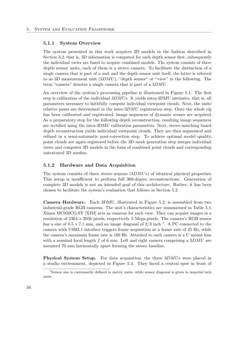
The system presented in this work acquires 3D models in the fashion described inSection 3.2, that is, 3D information is computed for each depth sensor first, subsequentlythe individual views are fused to acquire combined models. The system consists of threedepth sensor units, each of them is a stereo camera. To facilitate the distinction of asingle camera that is part of a unit and the depth sensor unit itself, the latter is referredto as 3D measurement unit (3DMU), “depth sensor“ or “view” in the following. Theterm “camera” denotes a single camera that is part of a 3DMU .
An overview of the system’s processing pipeline is illustrated in Figure 5.1. The firststep is calibration of the individual 3DMUs. It yields intra-3DMU intrinsics, that is, allparameters necessary to faithfully compute individual viewpoint clouds. Next, the units’relative poses are determined in the inter-3DMU registration step. Once the whole righas been calibrated and registrated, image sequences of dynamic scenes are acquired.As a preparatory step for the following depth reconstruction, resulting image sequencesare rectified using the intra-3DMU calibration parameters. Next, stereo matching baseddepth reconstruction yields individual viewpoint clouds. They are then segmented andrefined in a semi-automatic post-correction step. To achieve optimal model quality,point clouds are again registered before the 3D mesh generation step merges individualviews and computes 3D models in the form of combined point clouds and correspondinguntextured 3D meshes.
5.1.2 Hardware and Data Acquisition
The system consists of three stereo sensors (3DMUs) of identical physical properties.This setup is insufficient to perform full 360-degree reconstructions. Generation ofcomplete 3D models is not an intended goal of this architecture. Rather, it has beenchosen to facilitate the system’s evaluation that follows in Section 5.2.
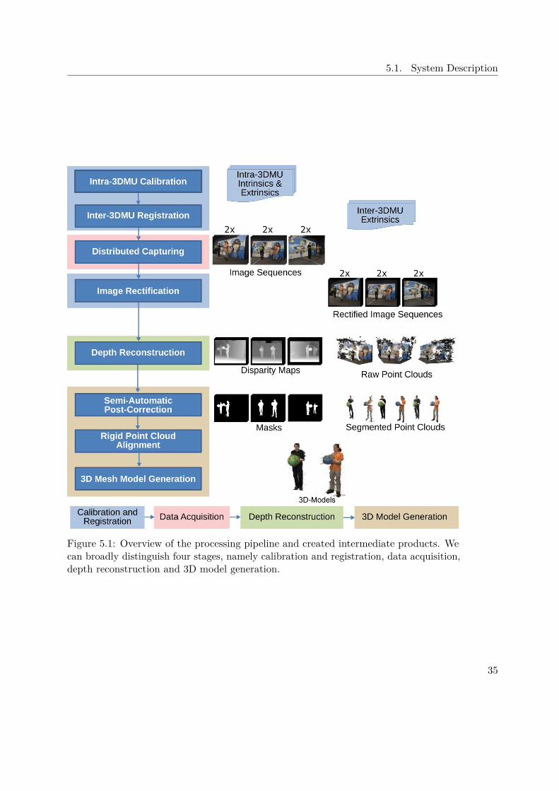
Camera Hardware. Each 3DMU, illustrated in Figure 5.2, is assembled from twoindustrial-grade RGB cameras. The unit’s characteristics are summarised in Table 5.1.Ximea MC050CG-SY [XIM] acts as cameras for each view. They can acquire images in aresolution of 2464 × 2056 pixels, respectively 5 Mega-pixels. The camera’s RGB sensorhas a size of 8.5 × 7.1 mm, and an image diagonal of 2/3 inch 1. A PC connected to thecamera with USB3.1 interface triggers frame acquisition at a frame rate of 25 Hz, whilethe camera’s maximum frame rate is 100 Hz. Attached to each camera is a C mount lenswith a nominal focal length f of 6 mm. Left and right camera comprising a 3DMU aremounted 70 mm horizontally apart forming the stereo baseline.
Physical System Setup. For data acquisition, the three 3DMUs were placed ina studio environment, depicted in Figure 5.4. They faced a central spot in front of
1Sensor size is customarily defined in metric units, while sensor diagonal is given in imperial inchunits.
34
5.1. System Description
Figure 5.1: Overview of the processing pipeline and created intermediate products. Wecan broadly distinguish four stages, namely calibration and registration, data acquisition,depth reconstruction and 3D model generation.
35
5. System and Evaluation Framework
Figure 5.2: Image of a 3D Measurement Unit (3DMU). It is a stereo camera comprisingtwo Ximea MC050CG-SY [XIM] industrial-grade cameras.
Camera properties Unit Value
Camera model Ximea MC050CG-SY [XIM]Lens mount CInterface USB 3.1Sensor dynamic range (used/max) bits per pixel 8/12Sensor size/diagonal mm 8.5 × 7.1/11.1Sensor size inch 2/3Camera resolution pix / Mpix 2464 × 2056 / 5.0Frame rate (used/max) Hz 25/100Lens focal length f mm 6Stereo baseline B mm 70
Table 5.1: System hardware characteristics.
the background that was at roughly 4 meter distance away. The main unit, 3DMU2,was placed approximately orthogonally to the planar scene background. 3DMU1 wassituated 2.2 m rightwards, and 3DMU3 2.4 m leftwards to the main unit. Ground truthmeasurements of the relative unit placement where taken with a measurement tape (seeAppendix A). In addition to ambient light from three windows, additional studio lightsilluminated the scene. Camera lenses were adjusted with the help of a preview and imagehistogram. Lens apertures were set such that the image intensity values covered thewhole histogram, while simultaneously avoiding overexposed image regions. Next, thelens focal points were jointly adjusted to have the scene’s center spot in focus. Finally,the camera’s white balance was carefully set to have the same chromatic properties in allviews.
Data Acquisition. Once the system is calibrated and rectified (see Section 5.1.3),image sequences of dynamic scenes can be acquired. A single controlling PC is connectedvia Ethernet to three capturing PCs, each of which is handling acquisition for a single3DMU . The system time of all PCs is synchronised via the Network Time Protocol (NTP).
36

5.1. System Description
Figure 5.3: Illustration of the physical camera setup and scene distance. Thegreen circles denote the physical positions of the depth sensor units. 3DMU1
is positioned at (2214.64, −61.71, −481.90), 3DMU2 at (0, 0, 0) and 3DMU3 at(−2471.13, 85.6284, −1228.66) in millimeter units. The reconstructed scene is depicted aspoint cloud coloured by distance to the origin of the coordinate system in 3DMU2.
Figure 5.4: Physical system setup. The three 3DMUs were placed approximately 2meters apart facing the scene in roughly 4 meters camera distance. Controlling andcapturing PCs are shown in the back. Additional to the light provided by the windows,three studio lights with diffuser boxes were used to illuminate the captured scenes.
37
5. System and Evaluation Framework
The controlling PC starts and stops image acquisition by sending respective messages viathe User Datagram Protocol (UDP) to the capturing PCs. Upon simultaneous receptionof the start message, capturing PCs start a local timer and periodically trigger frameacquisition of the attached cameras at a frequency of 25 frames per second. Images thatarrive at the PCs in raw sensor format are first converted into the RGB colour space, andare then saved to hard disk as uncompressed bitmap files. This format was chosen forlossless storage, and to keep processing time low. At the end of acquisition, the controllersends a stop signal causing the capturing PCs to end capturing. Data acquisition of ascene yields sequences of RGB image pairs for each of the three units.
Failure Cases. Two major failure cases with respect to data acquisition can be identi-fied, namely image synchronisation and motion blur.
Image Synchronisation. One challenge in acquiring image sequences for depthreconstruction is image synchronisation. Stereo matching algorithms that recover depthinformation from dynamic scenes assume that images are acquired at the same time.This assumption does not always hold for the acquired data used in this work. An errorin the camera control software caused image sequences captured by individual viewsto be of diverging lengths. For the same scene, one camera would output a differentnumber of frames than others. An attempt to recover synchronous image sequences hasbeen made according to the following procedure. First, one camera, namely the left, ofeach 3DMU was chosen as the main image source. Then for each frame of the maincamera, a corresponding frame in the right view with minimum time difference to themain camera’s frame is chosen. This yields a “repaired” image sequence for a single3DMU . The same procedure was repeated to temporally align image sequences amongseveral 3DMUs. Looking at subsequent frames of each camera, we can observe relativemotion. Due to the fact that one camera captured the scene at a different point in timethan its corresponding camera, we can see different amounts of motion in one view of acamera pair than the other (see Figure 5.5 top left and mid). The restoration procedureintroduced another case of temporal misalignment. There, motion is present in one view,but none occurs in the other (Figure 5.5 top right). Disparity maps computed frominsufficiently synchronised image pairs exhibit temporal flickering, depth discontinuitieswithin objects, as well as missing disparity values (see Figure 5.5 bottom). Point cloudscomputed from such disparity maps show distortions in moving regions (see Figure 5.5bottom). Subsequently, the system evaluation in this work is restricted to the first frameof each acquired scene only. There, strict camera synchronisation has been found to bepresent, whereas it is usually lost in later scene sections. Consequently, the evaluation ofdynamic motion is not part of this work.
Motion Blur. Another factor determining the quality of acquired models is motionblur. A video camera captures a certain number of frames per fixed units of time. Itis measured in frames per second (FPS). Images are acquired by integrating photonshitting the image sensor for a certain amount of time, the exposure time. The camera
38
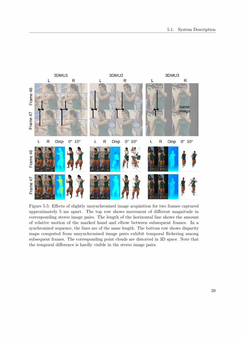
5.1. System Description
Figure 5.5: Effects of slightly unsynchronised image acquisition for two frames capturedapproximately 5 ms apart. The top row shows movement of different magnitude incorresponding stereo image pairs. The length of the horizontal line shows the amountof relative motion of the marked hand and elbow between subsequent frames. In asynchronized sequence, the lines are of the same length. The bottom row shows disparitymaps computed from unsynchronised image pairs exhibit temporal flickering amongsubsequent frames. The corresponding point clouds are distorted in 3D space. Note thatthe temporal difference is hardly visible in the stereo image pairs.
39

5. System and Evaluation Framework
(a) Input image (b) Disparity map (c) Point cloud
Figure 5.6: Illustration of motion blur in a scene containing fast movement. (a) Leftinput image; (b) Computed disparity map; (c) Point cloud.
FPS setting determines the maximum exposure time. For example, a camera capturingat 30 FPS frame rate has a maximum shutter speed of 33.3 ms. Any motion happeningseen by the camera in this time period is averaged in the same image. Borders of movingobjects appear blurred (i.e. motion blur). An example of this effect is illustrated inFigure 5.6. Borders of feet moving are almost completely blurred (Figure 5.6a). In thecomputed disparity map blurred areas are often assigned to the foreground, causing objectfattening, (Figure 5.6b). Corresponding point clouds (Figure 5.6c) contain erroneouspoints not belonging to the person’s foot, but rather to the background. At 25 fps,the feet of a slowly walking person appear blurred. It has been shown that movingpersons can be captured at 60 fps by state-of-the-art systems [DTK+16], whereas othersources [YGX+17] report failures already at 40 fps. Increasing the capture frame rateis one measure to cope with motion blur. Another approach is to keep the frame ratefixed, while decreasing the camera’s exposure time. A “staccato” effect can be observedin videos captured in this way. 3D reconstruction systems, however, use captured imagesnot as final output, but rather as an intermediate product for model generation. Thiseffect is not expected to play an important role in this application.
5.1.3 Calibration, Registration and Image Rectification
In order to perform depth reconstruction, first, individual camera parameters and depthsensor relative poses need to be determined. In our project, the method of Zhang [Zha00]is used to determine these parameters. Calibration and registration are performed beforethe actual image acquisition. The workflow is illustrated in Figure 5.7. It starts withestimating individual camera parameters. Next, relative poses of camera pairs withinindividual 3DMUs are determined, yielding the intra-3DMU calibration. It contains allparameters necessary to reconstruct models for each unit. Then camera poses of 3DMUsrelative to the main unit 3DMU2 are obtained, denoted as inter-3DMU registration.They facilitate later view fusion. Lastly, captured image sequences are rectified to allow
40
5.1. System Description
depth reconstruction by a stereo matching algorithm.
Intra-3DMU Calibration. We start by determining intra-3DMU calibration, andacquire all parameters necessary to reconstruct depth for a single view. For calibration,we use the camera model of the OpenCV [Bra00] library. Its camera model assumes thatno camera skew is present and uses the lens distortion model of Brown [Bro66].
Single Camera Calibration. Calibration images of a circle-grid pattern (see Figure 2.5b)are acquired while it is held in multiple poses. The asymmetric pattern grid has 4 rowsand 11 columns of circles. Circle center points are spread 50 mm apart between rowsand 25 mm between columns. Image coordinates of the circle centers are detected fromthe captured calibration images. Together with the known planar 3D coordinates of thecircle grid, a system of equations is formulated, whose solution yields the camera focallengths f i
xv, f iyv
and principle points cixv, ci
yvfor each camera v ∈ l, r of 3DMUi. They
can be represented as camera matrix:
Kiv =
f ix 0 ci
x
0 f iy ci
y
0 0 1
(5.1)
The skew parameter of Kiv is assumed to be 0. Lens distortion coefficients are given as
distiv = (ki
1v, ki2v, ki
3v, pi1v, pi
2v) as defined in Section 2.2.2 for each camera. In the project,the calibration process is initialised with a known nominal lens focal length of 6 mm(see Table 5.1) for both x and y dimensions to assist the calibration procedure in thedetermination of focal lengths, principal points and lens distortion. Said parameters arethen computed by invoking the function cv::calibrateCamera().
Stereo Camera Calibration. Next, relative poses of cameras within individual 3DMUsare obtained. Here, in the project OpenCV’s cv::stereoRectify() function is used.It yields rotation- and translation-vectors Ri and T i, respectively. They describe therectifying transformation aligning image planes of the left view caml
i and right view camri
belonging to 3DMUi, and put corresponding epipolar lines onto the same horizontalimage lines. Figure 5.8 illustrates the involved transformations. Note that the translationvectors point from camr
i to camli. After image rectification, a 3D world point at distance
infinity will have a value of 0 in the computed disparity maps. To keep the same imagesize along the whole processing pipeline, and to avoid aggressive image interpolation,applying the rectifying transformation warps captured image content into a sub-region ofthe original image. Stereo camera calibration describes these regions as bounding boxesfor the left, ROIi
l and the right, ROIir views of 3DMUi.
Finally, we have fully parameterised the individual camera geometry. For each 3DMUi,i ∈ 1, 2, 3, the set Intri = (Ki
l ∪ distil) ∪ (Ki
r ∪ distir) ∪ Ri ∪ T i ∪ ROIi
l ∪ ROIir is then
called the intra-3DMU calibration of the depth sensor 3DMUi.
Camera Registration. Once we know the intra-3DMU calibration, we can determinerelative poses between individual 3DMUs. We choose the middle depth sensor, 3DMU2,
41
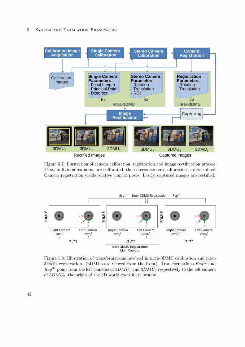
5. System and Evaluation Framework
Figure 5.7: Illustration of camera calibration, registration and image rectification process.First, individual cameras are calibrated, then stereo camera calibration is determined.Camera registration yields relative camera poses. Lastly, captured images are rectified.
yz
x
Left CameraRight Camera
3D
MU
1
caml1camr
1
[R1,T1]
yz
x
3D
MU
2
Left CameraRight Cameracaml
2camr2
[R2,T2]
yz
x
3D
MU
3
Left CameraRight Cameracaml
3camr3
[R3,T3]
Main Camera
Reg12 Reg32Inter-3DMU Registration
Intra-3DMU Registration
Figure 5.8: Illustration of transformations involved in intra-3DMU calibration and inter-3DMU registration. (3DMUs are viewed from the front). Transformations Reg12 andReg32 point from the left cameras of 3DMU1 and 3DMU3 respectively to the left cameraof 3DMU2, the origin of the 3D world coordinate system.
42
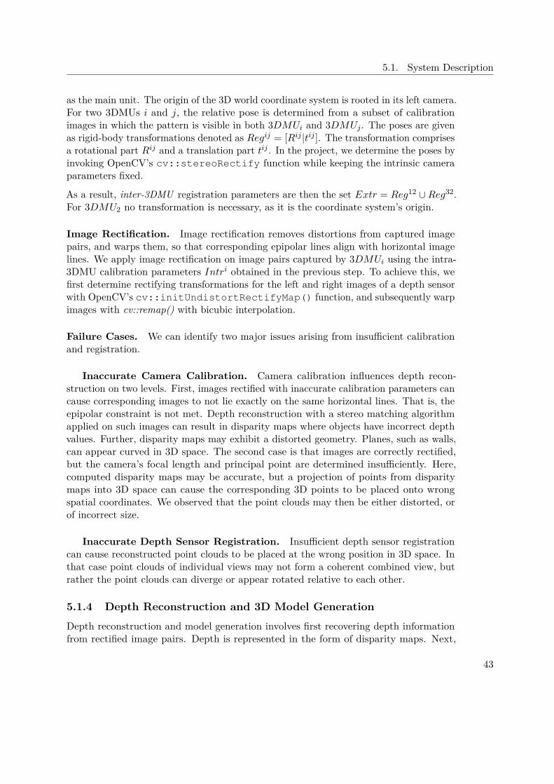
5.1. System Description
as the main unit. The origin of the 3D world coordinate system is rooted in its left camera.For two 3DMUs i and j, the relative pose is determined from a subset of calibrationimages in which the pattern is visible in both 3DMUi and 3DMUj . The poses are givenas rigid-body transformations denoted as Regij = [Rij |tij ]. The transformation comprisesa rotational part Rij and a translation part tij . In the project, we determine the poses byinvoking OpenCV’s cv::stereoRectify function while keeping the intrinsic cameraparameters fixed.
As a result, inter-3DMU registration parameters are then the set Extr = Reg12 ∪ Reg32.For 3DMU2 no transformation is necessary, as it is the coordinate system’s origin.
Image Rectification. Image rectification removes distortions from captured imagepairs, and warps them, so that corresponding epipolar lines align with horizontal imagelines. We apply image rectification on image pairs captured by 3DMUi using the intra-3DMU calibration parameters Intri obtained in the previous step. To achieve this, wefirst determine rectifying transformations for the left and right images of a depth sensorwith OpenCV’s cv::initUndistortRectifyMap() function, and subsequently warpimages with cv::remap() with bicubic interpolation.
Failure Cases. We can identify two major issues arising from insufficient calibrationand registration.
Inaccurate Camera Calibration. Camera calibration influences depth recon-struction on two levels. First, images rectified with inaccurate calibration parameters cancause corresponding images to not lie exactly on the same horizontal lines. That is, theepipolar constraint is not met. Depth reconstruction with a stereo matching algorithmapplied on such images can result in disparity maps where objects have incorrect depthvalues. Further, disparity maps may exhibit a distorted geometry. Planes, such as walls,can appear curved in 3D space. The second case is that images are correctly rectified,but the camera’s focal length and principal point are determined insufficiently. Here,computed disparity maps may be accurate, but a projection of points from disparitymaps into 3D space can cause the corresponding 3D points to be placed onto wrongspatial coordinates. We observed that the point clouds may then be either distorted, orof incorrect size.
Inaccurate Depth Sensor Registration. Insufficient depth sensor registrationcan cause reconstructed point clouds to be placed at the wrong position in 3D space. Inthat case point clouds of individual views may not form a coherent combined view, butrather the point clouds can diverge or appear rotated relative to each other.
5.1.4 Depth Reconstruction and 3D Model Generation
Depth reconstruction and model generation involves first recovering depth informationfrom rectified image pairs. Depth is represented in the form of disparity maps. Next,
43
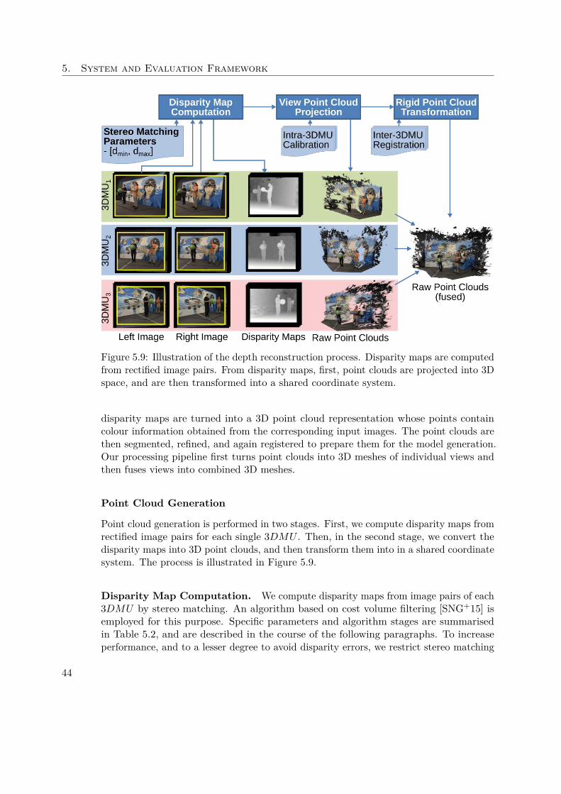
5. System and Evaluation Framework
Figure 5.9: Illustration of the depth reconstruction process. Disparity maps are computedfrom rectified image pairs. From disparity maps, first, point clouds are projected into 3Dspace, and are then transformed into a shared coordinate system.
disparity maps are turned into a 3D point cloud representation whose points containcolour information obtained from the corresponding input images. The point clouds arethen segmented, refined, and again registered to prepare them for the model generation.Our processing pipeline first turns point clouds into 3D meshes of individual views andthen fuses views into combined 3D meshes.
Point Cloud Generation
Point cloud generation is performed in two stages. First, we compute disparity maps fromrectified image pairs for each single 3DMU . Then, in the second stage, we convert thedisparity maps into 3D point clouds, and then transform them into in a shared coordinatesystem. The process is illustrated in Figure 5.9.
Disparity Map Computation. We compute disparity maps from image pairs of each3DMU by stereo matching. An algorithm based on cost volume filtering [SNG+15] isemployed for this purpose. Specific parameters and algorithm stages are summarisedin Table 5.2, and are described in the course of the following paragraphs. To increaseperformance, and to a lesser degree to avoid disparity errors, we restrict stereo matching
44

5.1. System Description
Algorithm Stage Method Parameter Value
Cost computation Census [ZW94] W=5 × 5Cost aggregation Permeability Filter [ÇığlaAA13] σ = 12Disparity post-processing Left-right consistency check Threshold: 0Hierarchical Matching [SNG+15] Levels: 0-2Temporal filtering Permeability Filter [ÇığlaAA13] σ = 12, σt = 1
Table 5.2: Stereo matching parameters used for disparity map computation.
to image areas containing active valid pixels. They are given as part of the intra-3DMUcalibration (see Section 5.1.3) and are denoted by ROIi
l and ROIir.
Cost Computation. Matching costs are computed with the Census [ZW94] simi-larity measure (see Section 3.2.1). Here, it measures the dissimilarity or costs betweentwo potentially corresponding pixels in left and right images of a pair. A local rectangularwindow of 5 × 5 size centered around pixels is taking into account for matching costcomputation.
Cost Volume. The per-pixel matching costs are stored in a three-dimensionalmatrix, the cost volume, of dimensions W × H × D in pixel units. W and H denoteimage width and height, and D = |dmax − dmin| is the size of the disparity search range(dmin, dmax). The disparity search range is given to the algorithm as input parameter,and has to be chosen the corresponding to minimum and maximum disparity valuesoccurring in the rectified image pairs. Note that disparity map values computed by thesystem are negative numbers, and consequently dmax denotes the disparity value of thefarthest point considered, while dmin denotes the value of the nearest point.
Cost Aggregation and Disparity Selection. The cost volume is then filteredin the cost aggregation step with the edge preserving permeability filter [ÇığlaAA13].The disparity value for a pixel p is selected with the common Winner-takes-it-all (WTA)strategy. Out of all D possible disparity values in the cost volume at position of pixel p,the one with minimum matching costs C(p, d) is chosen:
d(p) = argmind∈DC(p, d) (5.2)
Hierarchical Matching Scheme. Disparity estimation is embedded in a hierar-chical matching scheme to improve run-time and quality of the result. For each imagepair, a Gaussian image pyramid with k = 3 layers is built. Stereo matching is firstperformed on the coarsest layer l2. Images in this layer have a resolution of W
22 × H22 pixels.
Based on this initial disparity map, an offset map is computed that guides disparityestimation on the next finer layer l1 on images with W
21 × H21 pixels resolution. The process
45

5. System and Evaluation Framework
is then repeated for the finest layer l0 of the Gaussian pyramid with images of nativeresolution.
Consistency Checking. Next, inconsistent disparity map values are removed witha left-right consistency check. To do so, in addition to the original disparity map Dlr, asecond disparity map Drl is computed with the right view as the reference image. Anypixels whose corresponding disparity values differ between Dlr and Drl by more than athreshold value τ are marked as invalid. Here, τ is set to 0, to minimise the number oferroneously computed pixels.
Sub-pixel Refinement. In the cost volume approach possible disparity values arerepresented as slices of the cost volume. WTA disparity selection chooses as disparitythe index of the slice with minimum costs, yielding integral values. This leads to pointsbeing arranged along discrete planes in the corresponding point clouds. An enhancementstep recovers sub-pixel accuracy for each pixel p with disparity d by fitting a paraboliccurve through neighbouring cost values at p’s position in the cost volume [YYDN07].
dsp(p) = d −C(p, d + 1) − C(p, d − 1)
2 × (C(p, d − 1) + C(p, d + 1) − 2 × C(p, d))(5.3)
where dsp denotes the interpolated disparity value of pixel p at sub-pixel precision.
Temporal Filtering. Slightest changes in capturing conditions can lead to tempo-ral noise between subsequent frames of a video sequence. In order to reduce it, temporalfiltering with the permeability filter is applied. The cost penalties approach of [ÇığlaAA12]is used. Specifically, the cost volume is updated with a temporal consistency term. First,the temporal change of each pixel in terms of its RGB value is determined by computingits permeability weight µt:
µt = min(e−∆R
σ , e−∆G
σ , e−∆B
σ ) (5.4)
where ∆R, ∆G, ∆B denote the absolute difference between R, G and B channel valuesof a pixel in two subsequent image frames, and σ is the permeability filter smoothingfactor. A pixel’s permeability weight µt determines the ratio of pixels to be transferredfrom the previous to the next frame. µt is high for pixels with similar RGB values, thosein non-moving areas, and low for pixels in fast moving areas, as they have diverging RGBvalues. Next, the cost volume is updated. For each pixel p = (x, y) at disparity value dand costs C(p, d), updated costs Ct(p, d) are computed as:
Ct(p, d) + µt × |d − dt−1(p)| × σt (5.5)
where dt−1 is the disparity value of p at the previous frame. σt is a temporal smoothingfactor. For pixels in fast moving regions, those with high permeability weight, the newdisparity value is favoured, while for pixels in non-moving areas disparity values changesmoothly from one frame to the next. The temporal smoothing factor σt is set to 1.
46
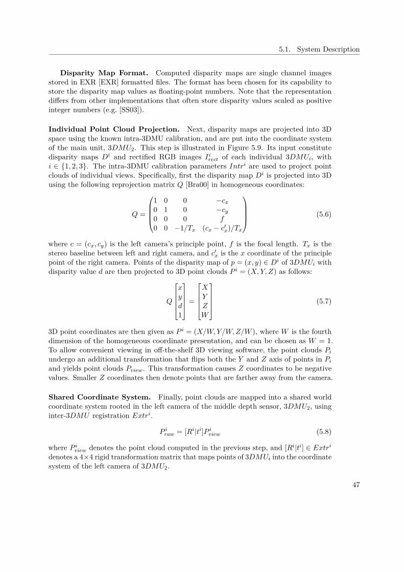
5.1. System Description
Disparity Map Format. Computed disparity maps are single channel imagesstored in EXR [EXR] formatted files. The format has been chosen for its capability tostore the disparity map values as floating-point numbers. Note that the representationdiffers from other implementations that often store disparity values scaled as positiveinteger numbers (e.g. [SS03]).
Individual Point Cloud Projection. Next, disparity maps are projected into 3Dspace using the known intra-3DMU calibration, and are put into the coordinate systemof the main unit, 3DMU2. This step is illustrated in Figure 5.9. Its input constitutedisparity maps Di and rectified RGB images Ii
rect of each individual 3DMUi, withi ∈ 1, 2, 3. The intra-3DMU calibration parameters Intri are used to project pointclouds of individual views. Specifically, first the disparity map Di is projected into 3Dusing the following reprojection matrix Q [Bra00] in homogeneous coordinates:
Q =
1 0 0 −cx
0 1 0 −cy
0 0 0 f0 0 −1/Tx (cx − c′
x)/Tx
(5.6)
where c = (cx, cy) is the left camera’s principle point, f is the focal length. Tx is thestereo baseline between left and right camera, and c′
x is the x coordinate of the principlepoint of the right camera. Points of the disparity map of p = (x, y) ∈ Di of 3DMUi withdisparity value d are then projected to 3D point clouds P i = (X, Y, Z) as follows:
Q
xyd1
=
XYZW
(5.7)
3D point coordinates are then given as P i = (X/W, Y/W, Z/W ), where W is the fourthdimension of the homogeneous coordinate presentation, and can be chosen as W = 1.To allow convenient viewing in off-the-shelf 3D viewing software, the point clouds Pi
undergo an additional transformation that flips both the Y and Z axis of points in Pi
and yields point clouds Pview. This transformation causes Z coordinates to be negativevalues. Smaller Z coordinates then denote points that are farther away from the camera.
Shared Coordinate System. Finally, point clouds are mapped into a shared worldcoordinate system rooted in the left camera of the middle depth sensor, 3DMU2, usinginter-3DMU registration Extri.
P iraw = [Ri|ti]P i
view (5.8)
where P iview denotes the point cloud computed in the previous step, and [Ri|ti] ∈ Extri
denotes a 4×4 rigid transformation matrix that maps points of 3DMUi into the coordinatesystem of the left camera of 3DMU2.
47

5. System and Evaluation Framework
The output of the point cloud projection constitute point clouds P iraw = (X, Y, Z, R, G, B)
where X,Y , and Z are coordinates in the shared coordinate system, and R,G,B are red,green and blue colour channel values obtained from the corresponding input images Ii
rect.The point clouds P i
raw are stored in the PLY [PLY] format.
Rigid Point Cloud Registration
The relative pose between individual views (see Section 5.1.3) is refined in the 3D domainon a per scene basis to achieve optimal view overlap. An example of the updatedregistration and its effect on the scene is shown in Figure 5.10. The refined registrationshifts points of 3DMU3 to the right, and removes duplication of the right person’sfront. As input for rigid point cloud registration, a segmented point cloud containingonly the object P i
raw reconstructed from 3DMU1 and 3DMU2 is aligned to the static3DMU2. The point clouds are registered by our project partners using a variant of theSuper4PCS [MAM14] algorithm that takes point coordinates, as well as points’ RGBcolour information, into account. This process results in two rigid body transformationsT 12
corr and T 32corr. Applying these transformations to 3DMU1 and 3DMU3 brings them
into optimal alignment with 3DMU2.
Semi-automatic Post-Correction
A custom interactive software application, developed outside of the scope of this work,is used to process and examine point clouds based on previously computed disparitymaps (see Section 5.1.4). The application serves multiple purposes. First, it enables thecreation of segmentation masks that identify scene regions that serve as input for modelgeneration. Next, it creates registered and corrected individual viewpoint clouds. Lastly,it contains several tools for point cloud refinement, such as cleaning point clouds fromoutliers.
Image Segmentation Although models for the whole captured scene can be generated,usually, only parts of the scene are of interest. Identification of these areas is done bycreating segmentation masks. The user draws coarse annotations (i.e. “scribbles”) overtarget objects (Figure 5.11a). Two kinds of scribbles can be drawn, namely foreground-and background-scribbles. They identify object- and background-regions, respectively.Scribbles are interactively expanded using a model [Bro16] that incorporates colour-information from the view’s input image, as well as depth-cues from disparity maps. Toassist the user, scribbles can be propagated onto the views of other 3DMUs, employinginter-3DMU registration. The same model [Bro16] allows the propagation of drawnscribbles temporally over several image frames, and facilitates video segmentation. Oncethe user is satisfied with the annotation, scribbles are then converted into object masks(see Figure 5.11b). In another step, the computed object masks are then propagatedtemporally to subsequent frames of a temporal sequence. The application contains severaltools, to facilitate accurate mask generations. Among them are morphological operations,
48
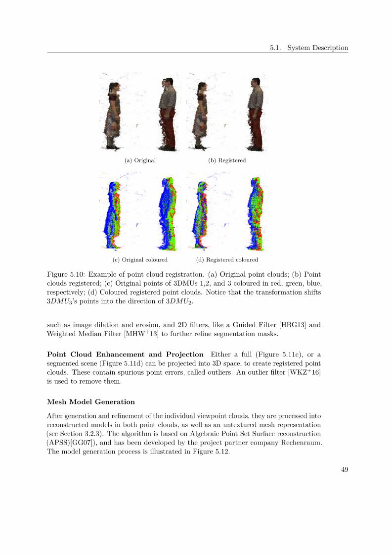
5.1. System Description
(a) Original (b) Registered
(c) Original coloured (d) Registered coloured
Figure 5.10: Example of point cloud registration. (a) Original point clouds; (b) Pointclouds registered; (c) Original points of 3DMUs 1,2, and 3 coloured in red, green, blue,respectively; (d) Coloured registered point clouds. Notice that the transformation shifts3DMU3’s points into the direction of 3DMU2.
such as image dilation and erosion, and 2D filters, like a Guided Filter [HBG13] andWeighted Median Filter [MHW+13] to further refine segmentation masks.
Point Cloud Enhancement and Projection Either a full (Figure 5.11c), or asegmented scene (Figure 5.11d) can be projected into 3D space, to create registered pointclouds. These contain spurious point errors, called outliers. An outlier filter [WKZ+16]is used to remove them.
Mesh Model Generation
After generation and refinement of the individual viewpoint clouds, they are processed intoreconstructed models in both point clouds, as well as an untextured mesh representation(see Section 3.2.3). The algorithm is based on Algebraic Point Set Surface reconstruction(APSS)[GG07]), and has been developed by the project partner company Rechenraum.The model generation process is illustrated in Figure 5.12.
49
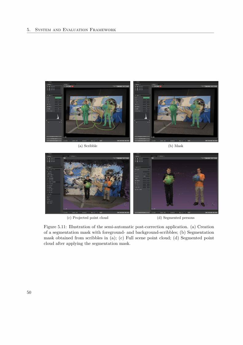
5. System and Evaluation Framework
(a) Scribble (b) Mask
(c) Projected point cloud (d) Segmented persons
Figure 5.11: Illustration of the semi-automatic post-correction application. (a) Creationof a segmentation mask with foreground- and background-scribbles; (b) Segmentationmask obtained from scribbles in (a); (c) Full scene point cloud; (d) Segmented pointcloud after applying the segmentation mask.
50
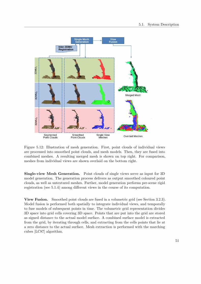
5.1. System Description
Figure 5.12: Illustration of mesh generation. First, point clouds of individual viewsare processed into smoothed point clouds, and mesh models. Then, they are fused intocombined meshes. A resulting merged mesh is shown on top right. For comparison,meshes from individual views are shown overlaid on the bottom right.
Single-view Mesh Generation. Point clouds of single views serve as input for 3Dmodel generation. The generation process delivers as output smoothed coloured pointclouds, as well as untextured meshes. Further, model generation performs per-scene rigidregistration (see 5.1.4) among different views in the course of its computation.
View Fusion. Smoothed point clouds are fused in a volumetric grid (see Section 3.2.3).Model fusion is performed both spatially to integrate individual views, and temporallyto fuse models of subsequent points in time. The volumetric grid representation divides3D space into grid cells covering 3D space. Points that are put into the grid are storedas signed distance to the actual model surface. A combined surface model is extractedfrom the grid, by iterating through cells, and extracting from the cells points that lie ata zero distance to the actual surface. Mesh extraction is performed with the marchingcubes [LC87] algorithm.
51
5. System and Evaluation Framework
Failure Cases
Depth reconstruction is an ill-posed problem, and is consequently prone to errors. Wecan broadly identify two major areas that can cause inaccurate results. The first has todo with artefacts introduced in disparity map computation. The second area lies in meshmodel generation and subsequent fusion of the single views.
Depth Reconstruction Artefacts. Stereo matching recovers scene depth by identify-ing pixels belonging to the same imaged objects in image pairs. In addition to occlusions,that is pixels, which are only visible in one of the two images, untextured regions, such asevenly white walls, and specular or transparent image regions often cause stereo matchingalgorithms produce erroneous matches. When disparity maps are projected into 3D spaceas point clouds, inaccuracies become more prominent. Disparity map noise within anobject is translated to ill-defined surfaces in point clouds. This makes reconstructionof fine object features challenging. In the example of the dancer’s head depicted inFigure 5.13, facial features like nose and cheeks are hard to distinguish in the pointcloud. Subsequent 3D model generation also applies outlier detection and smoothing tofit smooth surfaces onto the remaining points. In our example, this causes the nose toappear flattened in the computed mesh model. The reverse effect can be observed on thechin. It appears more pronounced than it is in reality. For larger objects, the amountof point cloud noise poses a lesser problem, as can be seen on the torso in Figure 5.14.The high amount of smoothing necessary to recover other, more delicate areas, however,leads to spurious bumps, as can be seen at the arms.
View Fusion Artefacts. View fusion is performed to achieve complete models. Thefusion method has to cope with overlapping, and slightly misaligned regions. Theperson’s feet in the overlaid mesh shown in Figure 5.12 give an example of such amisalignment occurring despite careful unit pose registration, and per-scene re-registration.Misalignment can lead to degraded models that exhibit duplication of misaligned features.This issue can be mitigated by iteratively updating pose registration on a frame-by-framebasis from reconstructed model data [ZSG+18]. Another type of artefact occurringwhile fusing models are chromatic misalignments. Model colours diverge slightly inthe individual views due to differing illumination conditions at respective depth sensorpositions. Careful chromatic alignment of the capturing cameras is not sufficient toeliminate this effect. Some state-of-the-art systems, such as [DCC+18], additionallyperform chromatic alignment by creating linear colour mapping among the views offline,and applying them to the captured images. The generated meshes are untextured. Theyare textured by simple colour interpolation from the corresponding smoothed pointcloud. In order to acquire high resolution texture and to eliminate ridges in fusedmodel textures, more sophisticated texture stitching approaches need to be applied,e.g. [EFR+17, DCC+18]. Accurate texture reproduction, however, was outside of thescope of the examined system.
52

5.1. System Description
Figure 5.13: Detailed views of the dancers1 data set. Input point clouds, shown incolour and colour-coded by capturing 3DMU , are noisy in small local regions, like thehead. Output point clouds are aggressively smoothed (middle). The mesh output isinitially untextured. Texture information is added by colour interpolation from theoutput point cloud.
(a) 3DMU3 (b) 3DMU2 (c) 3DMU1 (d) Merged Points
Figure 5.14: Illustration of model artefacts introduced by views. 3DUM3 (a) introducesbumps on the back. While 3DMU2 (b) captures the persons nose accurately, 3DMU1
captures no distinct nose. Chromatic artefacts in the final mesh (d) are introduced bysimple colour interpolation.
53
5. System and Evaluation Framework
5.1.5 Summary
In this section, the examined system has been described in detail along the processingpipeline’s major building blocks. First a high-level overview of the processing pipelineand processing steps has been given. Then, the individual stages depth acquisition,calibration and registration, and depth reconstruction have been discussed. Further,challenges and failure cases that can arise at the respective steps have been discussed.
5.2 Evaluation Strategies
This section describes the evaluation methods used to evaluate the system described inSection 5.1. It is structured as follows. Section 5.2.1 lays out the evaluation on validationobjects. Next, in Section 5.2.2 the novel view evaluation method is described. Lastly,Section 5.2.3 covers the design of the user study conducted in this work.
5.2.1 Evaluation on Validation Objects
Ideally, 3D reconstruction recovers metric properties of the captured scene. Lengths andangles measured on real objects are the same as on their reconstructed counterparts.Any given real system inevitably exhibits deviations from the ideal situation. Goal of theground truth evaluation is to quantify these deviations, and to characterise the system’sability to recover metric properties of captured objects. We consider two different typesof objects.
The first type are spherical objects. From a geometric perspective, spheres are simplebodies that can be defined only by their position in 3D space and their radius. Recon-struction of spheres, however, can be challenging, since, apart from their outline, they donot exhibit any distinct geometric features. An important measure is the distribution ofdeviation of sampled points compared to their ideal position. Depth- as well as surfacereconstruction algorithms often perform filtering that can lead to sphere models notbeing round but rather “bumpy”.
The second type of object examined are cuboid bodies, that is boxes. Adjacent faces of abox join in a 90 deg angle. Deviations from this angle allow us to identify spatial skew inthe reconstruction.
The evaluation on validation objects will be carried out in the following manner:
1. Creation of validation objects Spherical and cuboid objects will be created.Special care will be put into the quality of their surfaces, as they need do beproperly acquired by the system. Another consideration is their size. They will bemade large enough, so they that their reconstructions comprise sufficiently manysample points. For spheres, the measured diameter will be used as ground truthvalue.
54
5.2. Evaluation Strategies
2. Validation object acquisition The objects will then be acquired with the system.Samples from various object positions will be taken, in order to get diverse dataset.
3. Object segmentation A semi-automatic post-correction application (see Sec-tion 5.1.4) will then be used to segment out only points constituting the validationobjects. For spheres, the whole visible sphere area is considered. For boxes, faceswill be segmented separately to allow plane fitting on each face. After segmentation,point clouds only consisting of the object areas will be generated.
4. Shape Fitting Validation object point cloud samples will undergo a shape fittingprocess. For spherical objects, an ideal sphere with measured true sphere radiuswill be fitted into the point cloud samples, determining the position in space thatbest fits the sample. For cuboid objects, plane fitting will determine the planeoptimally describing the orientation of each face. Shape fitting is performed forsphere and planes by means of the non-linear least squares optimisation [Sha98].The sphere fitting procedure is performed by our project partner.
5. Analysis of shape fitting results Once the ground truth data set is available,deviations from ground truth measurements will be determined. The signed errorbetween the distance of a reconstructed point to the fitted sphere center and thesphere’s true radius is determined. Another area of interest is the relation betweenthe signed distance error and the distance of the object to the camera.
5.2.2 Novel View Evaluation
For novel view evaluation, we adopt the image-based virtual rephotography methodproposed in [WBF+17] that has been described in Section 4.2. The goal of this evaluationis to determine the quality of intermediate and final reconstruction products in terms ofsimilarity to the input images of the reconstruction process. Selected input images serveas ground truth against which the reconstruction products are compared.
1. Data set acquisition Representative scenes of persons are acquired and processedinto 3D models. Several variants are created to examine their performance ondifferent variants of model generation. A full description of the considered variantsis given in Section 6.1.2. For each variant and model, original point clouds, smoothedpoint clouds, and textured meshes are prepared for examination. The use of theseproducts allows to track the results of individual processing steps over the courseof the reconstruction process.
2. Novel view generation Next, novel view images of the created products arerendered into the viewpoint of each depth sensor, such that the novel view imagesideally show the exact same content as the respective rectified input image. Viewgeneration takes into account intra-3DMU calibration parameters to determine
55
5. System and Evaluation Framework
the corresponding field-of-view, as well as inter-3DMU registration to replicate thepose of the capturing depth sensor camera.
3. Accuracy computation Then, the accuracy of all products and variants is de-termined. Accuracy is defined as the similarity between the (rectified) image ofthe depth sensor’s left camera and the novel-view image of the corresponding prod-uct. For similarity computation, the normalised cross coefficient (NCC) measureis chosen due to its robustness to illumination and exposure changes. Further,the NCC measure has been shown to correlate to user opinions in subjectiveevaluations [WBF+17] on 3D reconstructed models.
Similarity is computed in the masked region used for segmentation of the foregroundmodels from the scene background. NCC values are linearly transformed into the[0, 1] value range, so that a value of 0 indicates total dissimilarity, and 1 identity ofcompared images. A window size of 30 pixels is used for similarity computation.
Model completeness is determined for all comparisons. It is defined as the ratio ofvalid mask pixels with respect to the total numbers of image pixels. Waechter etal. [WBF+17] deem reporting of completeness ratios as necessary in conjunctionwith accuracy, for fair comparison.
4. Analysis of similarity results Model completeness is reported for each model.For accuracy, two specific cases are considered, reconstruction at the original cameraposition and reconstruction at a novel view. In the first case, the accuracy of eachdepth sensor is determined with views corresponding the original sensor’s position.In the second case, models that have been fused from the two outermost views3DMU1 and 3DMU3 are compared against the reference view 3DMU2. Since dataof the reference view is not part of the compared models, it can be used as anindependent source of validation.
5.2.3 Subjective User Study
This section describes the experimental setup and design of the user study conductedfor this work. It serves two aims. The first is to assess how the participants rate thedesign of the proposed study. Its results will be used as feedback for the design of asubsequent larger study with more participants, which is outside the scope of this diplomathesis. The second goal is to compare different 3D model reconstruction methods interms of perceived model quality (see Section 6.1). The participants’ judgement is takenas measure for the quality of the selected reconstruction methods.
Testing Environment. A room was prepared to allow users to regard the testingmaterial without visual distraction. While the trial was in progress, the room was keptdarkened, so to achieve uniform and controlled illumination conditions. We set up atesting environment, shown in Figure 5.15, according to the requirements of [ITU12]. Alaptop was running a software developed for this purpose. The material was presentedon an uncalibrated monitor (Asus VG278) with a diagonal of 27 inch and a display
56
5.2. Evaluation Strategies
Figure 5.15: Illustration of the lab environment for subjective evaluation.
resolution of 1920 × 1080 pixels. The monitor’s white balance was set to 5000 Kelvin, itsbrightness was adjusted to a minimum. Participants were seated at approximately 0.9meter distance to the screen.
Testing Material. We rendered videos of textured 3D meshes in front of a non-uniform(violet to black) background. Each video was shown for a fixed time of 20 seconds. To allowviewers to concentrate on the models, the scene background was removed as described inSection 5.1.4 with the same segmentation masks as for the novel-view evaluation (seeSection 5.2.2). In the course of the video the camera’s viewpoint moves slowly on apath, and stops at certain positions for one second. The positions are those of the depthsensors capturing the models (see Section 5.1.2). A fourth, additional, viewpoint above3DMU2 is introduced as a novel viewpoint. This procedure is adopted for two reasons.First, it allows viewers to regard the material from different perspectives. Second, itavoids mental overload. Participants can concentrate on regarding the presented materialwithout having to navigate themselves within the scene. This aspect is especially helpfulfor naïve participants not familiar with navigation in 3D scenes.
Study Design. The Pair Comparison (PC) methodology described in Section 4.3 isadopted for this assessment. The study design is similar to that of [Nez14, NBSG14]. InPC, pairs of stimuli (e.g 3D models, videos, images, etc.) are displayed to the participants.They express their preference for one item of a pair with an “A is better than B” or “B isbetter than A” choice. Participants are also allowed to vote for “no preference” [LGE13],as the compared approaches can be similar. The trial sessions lasted for approximately40 minutes. One participant at a time was admitted to the trial.
A session comprises five stages, with the steps being (1) introduction, (2) screening, (3)practice, (4) experimental trial and (5) interview. Participants where briefly introducedorally, and where given written instructions in either English (see Figure B.1) or German
57
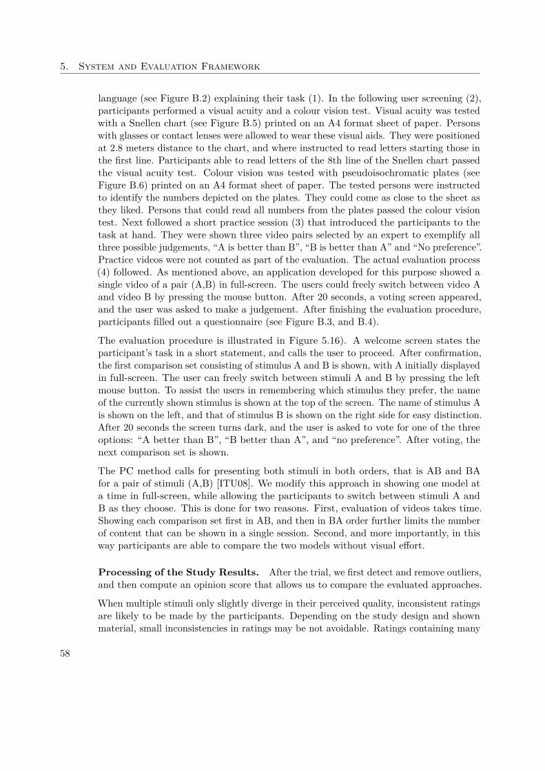
5. System and Evaluation Framework
language (see Figure B.2) explaining their task (1). In the following user screening (2),participants performed a visual acuity and a colour vision test. Visual acuity was testedwith a Snellen chart (see Figure B.5) printed on an A4 format sheet of paper. Personswith glasses or contact lenses were allowed to wear these visual aids. They were positionedat 2.8 meters distance to the chart, and where instructed to read letters starting those inthe first line. Participants able to read letters of the 8th line of the Snellen chart passedthe visual acuity test. Colour vision was tested with pseudoisochromatic plates (seeFigure B.6) printed on an A4 format sheet of paper. The tested persons were instructedto identify the numbers depicted on the plates. They could come as close to the sheet asthey liked. Persons that could read all numbers from the plates passed the colour visiontest. Next followed a short practice session (3) that introduced the participants to thetask at hand. They were shown three video pairs selected by an expert to exemplify allthree possible judgements, “A is better than B”, “B is better than A” and “No preference”.Practice videos were not counted as part of the evaluation. The actual evaluation process(4) followed. As mentioned above, an application developed for this purpose showed asingle video of a pair (A,B) in full-screen. The users could freely switch between video Aand video B by pressing the mouse button. After 20 seconds, a voting screen appeared,and the user was asked to make a judgement. After finishing the evaluation procedure,participants filled out a questionnaire (see Figure B.3, and B.4).
The evaluation procedure is illustrated in Figure 5.16). A welcome screen states theparticipant’s task in a short statement, and calls the user to proceed. After confirmation,the first comparison set consisting of stimulus A and B is shown, with A initially displayedin full-screen. The user can freely switch between stimuli A and B by pressing the leftmouse button. To assist the users in remembering which stimulus they prefer, the nameof the currently shown stimulus is shown at the top of the screen. The name of stimulus Ais shown on the left, and that of stimulus B is shown on the right side for easy distinction.After 20 seconds the screen turns dark, and the user is asked to vote for one of the threeoptions: “A better than B”, “B better than A”, and “no preference”. After voting, thenext comparison set is shown.
The PC method calls for presenting both stimuli in both orders, that is AB and BAfor a pair of stimuli (A,B) [ITU08]. We modify this approach in showing one model ata time in full-screen, while allowing the participants to switch between stimuli A andB as they choose. This is done for two reasons. First, evaluation of videos takes time.Showing each comparison set first in AB, and then in BA order further limits the numberof content that can be shown in a single session. Second, and more importantly, in thisway participants are able to compare the two models without visual effort.
Processing of the Study Results. After the trial, we first detect and remove outliers,and then compute an opinion score that allows us to compare the evaluated approaches.
When multiple stimuli only slightly diverge in their perceived quality, inconsistent ratingsare likely to be made by the participants. Depending on the study design and shownmaterial, small inconsistencies in ratings may be not avoidable. Ratings containing many
58
5.3. Summary
A
B
20 sec VoteA B=
Welcome Finish
Next Comparison Set
Figure 5.16: Illustration of the pair-based comparison scheme. The user is brieflyintroduced to the task on a welcome screen. Next, the first comparison set is shown,with one stimulus of a pair in full-screen. Users can freely switch between two stimuli bypressing the left mouse button. After 20 seconds, a gray screen appears calling to vote.
contradicting, or even random, judgements, however, are considered as outliers, and needto be excluded from consideration, so not to bias the evaluation results. We apply thealgorithm of [LGE13] to detect and reject outliers. It detects inconsistent judgements bycounting circular triads, that is inconsistent triples of stimuli preference. An example fora circular triad are three stimuli A, B and C together with the preferences A > B, B > Cand C > A, where the relation symbols < and > denote preference. A few inconsistentjudgements per participant are allowed. If the number of circular triads rises beyond athreshold, however, the judgement is to be excluded from statistical processing. Theratio of inconsistent judgements to the total number of judgements is referred to as thetransitivity satisfaction rate [LGE13].
For statistical processing, we first extract separate comparison sets for depth reconstruc-tion and view-fusion approaches from the combined comparison sets obtained from thetrials. To this end, we group judgements according to the respective type of comparedapproach. Following the approach of [NBSG14], we then transform the comparisonsets into continuous quality scores using the Bradley-Terry model [BT52], by maximumlikelihood estimation of a log-likelihood function. The converted quality scores and theirstandard deviation are then reported.
5.3 Summary
This chapter presented a description of the examined system and the applied evaluationmethods. The system consists of three RGB stereo-camera based depth sensors termed3DMU (3D measurement unit). Prior to model acquisition, the depth sensors arecalibrated and their poses relative to the middle (reference) view are determined. Stereo-image pairs are acquired in a synchronised and distributed fashion on multiple computers.A stereo matching algorithm recovers point clouds from image pairs of individual depthsensors. In a semi-automatic approach, point clouds of individual views are segmentedand cleaned from outliers. An APSS based surface reconstruction algorithm first createsrefined point clouds for each view and finally fuses them into combined mesh models.
The plan for evaluating the regarded multi-view 3D reconstruction system in terms of
59

5. System and Evaluation Framework
accuracy and model quality comprises two quantitative and one qualitative evaluation.The first approach uses acquisitions of specially crafted validation objects (sphere, box),to determine the geometric reproduction capabilities. Second, a novel view evaluationdetermines model accuracy by measuring image-based similarity on intermediate and finalsystem products. Lastly, a pair-based user study conducted in the course of this workdetermines the quality of several model reconstruction methods in terms of subjectiveuser opinions.
60
CHAPTER 6Evaluation Results
This chapter discusses the evaluation results in detail. First, Section 6.1.1 presents thedata set used for novel view evaluation and the user study. Next, Section 6.3 containsthe results of the novel view evaluation. Finally, Section 6.4 details the results of theuser study conducted for this work.
6.1 Data Set and Evaluated Approaches
6.1.1 Data Set
We have chosen five acquired models for evaluation (see Figure 6.1). Due to someacquisition limitations described in Section 5.1.2, only static models are considered inthe current evaluation. Several intermediate and final products, summarised in Table 6.1,are examined. From the three available views, we generate combined models consistingof views 3DMU1 and 3DMU3, while ignoring for now the view generated from 3DMU2.Combined versions are created for smoothed points and coloured meshes and are denotedin the following as view 3DMU1+3.
Product Description
Original points Input point cloud for model generationSmoothed points Intermediate point cloud created in model generationColoured meshes Created from final mesh output of model generation
Table 6.1: Products used for novel-view evaluation and user study. For a more detaileddescription see Section 5.1.4.
61
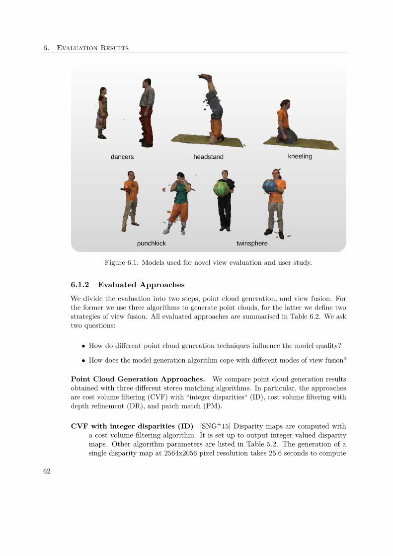
6. Evaluation Results
Figure 6.1: Models used for novel view evaluation and user study.
6.1.2 Evaluated Approaches
We divide the evaluation into two steps, point cloud generation, and view fusion. Forthe former we use three algorithms to generate point clouds, for the latter we define twostrategies of view fusion. All evaluated approaches are summarised in Table 6.2. We asktwo questions:
• How do different point cloud generation techniques influence the model quality?
• How does the model generation algorithm cope with different modes of view fusion?
Point Cloud Generation Approaches. We compare point cloud generation resultsobtained with three different stereo matching algorithms. In particular, the approachesare cost volume filtering (CVF) with “integer disparities“ (ID), cost volume filtering withdepth refinement (DR), and patch match (PM).
CVF with integer disparities (ID) [SNG+15] Disparity maps are computed witha cost volume filtering algorithm. It is set up to output integer valued disparitymaps. Other algorithm parameters are listed in Table 5.2. The generation of asingle disparity map at 2564x2056 pixel resolution takes 25.6 seconds to compute
62
6.2. Results of Evaluation on Validation Objects
a disparity map 1, and is the fastest of all considered methods. Integer valueddisparity maps exhibit discrete spatial resolution. In the derived point clouds, the3D points are grouped along few planes in Z axis direction. The model generationalgorithm has to cope with relatively few cues with respect to available depthinformation.
CVF with depth refinement (DR) [SNG+15] Disparity maps are computed withthe same algorithm as for the ID variant. Here, the disparity map is additionallyrefined using sub-pixel enhancement [YYDN07], and filtered with a weighted medianfilter [MHW+13]. Other algorithm parameters are listed in Table 5.2. Generationof a disparity map takes 71.37 seconds on average. DR disparity maps and derivedpoint clouds are dense, and locally noisy. The model generation algorithm has tocorrectly derive smooth surfaces from many points.
PatchMatch (PM) [LZYZ18] In contrast to CVF, PatchMatch derives disparity valuesby estimating slanted planes per pixel and then minimising a global energy function.Models are generated with the parameters set for the Middlebury 2006 benchmarkas described in [LZYZ18]. A notable difference to the paper is that we let thealgorithm run for 30 iterations, instead of the originally suggested 5. Disparitymap computation takes on average 25.8 minutes per view. PM disparity mapsand corresponding point clouds are already very smooth. The model generationalgorithm input data is optimal in terms of input noise.
View Fusion Approaches. We assess the quality of the model generation algorithmdescribed in Section 5.1.4) by comparing two different methods of view fusion:
Fuse views after model generation (FA). Here, we first generate single view mod-els, and afterwards fuse them. This method effectively performs a union operationon the regarded single views.
Fuse views before model generation (FB). In contrast to the previous approach,we fuse point clouds before model generation. Fused point clouds are treated as asingle view by the model generation algorithm.
6.2 Results of Evaluation on Validation Objects
In this evaluation, we want to determine the accuracy of reconstructed objects. Geometri-cally simple-shaped validation objects created for this purpose are acquired by the system.Then, ideal 3D models of same geometric properties are fitted into the reconstructedobject point clouds. We then obtain deviations of the acquired point clouds to the fitted
1A desktop PC with a 12 thread Intel i7-3930K CPU clocked at 3.2 GHz with 32 GB of RAM wasused for determining the computation times. The active area of the input images had a resolution ofapproximately 2200 × 1800 pixels. All methods were using multi-threaded CPU implementations.
63

6. Evaluation Results
Abbr. Description
ID CVF [SNG+15] integer disparities. No subpixel refinement, no depth refine-ment
DR CVF [SNG+15] floating point disparity. Subpixel refinement [YYDN07] anddepth refinement [MHW+13]
PM Patch Match [LZYZ18] floating point disparities
FB View point clouds are fused before model generationFA View point clouds are fused after model generation
Table 6.2: Evaluated approaches for novel view evaluation and user study.
models that serve as ground truth measurements. The method has been described inSection 5.2.1.
In particular we pose the following questions:
1. How accurate is the reconstruction of spherical objects in terms of outliers?
2. Does accuracy depend on the camera to object distance?
3. How accurate is the plane reconstruction of a cuboid?
6.2.1 Data Set and Validation Objects
Validation Objects Two spheres and one box were created for this evaluation. Theirsurfaces were designed to allow a robust reconstruction. Specifically, a primarily bluesphere of 150 mm radius and a green sphere of 185 mm radius serve as validation object(see the twinsphere model in Figure 6.1). A cardboard box serves as cuboid object(e.g. Figure 6.5).
Data Set We use raw point clouds that are produced by the depth-reconstructionstage of the system (see Section 5.1.4). The point clouds were generated with the DRapproach described in Section 6.1.2.
The sphere data set comprises 29 reconstructions of blue and green spheres. Out ofthese, 26 samples are used. 3 samples had to be dropped from the data set due to thesphere fitting algorithm not converging. Sphere point cloud samples ranged from 47500to 217872 points, with an average point count of 108189. The distance of the spheres tothe respective depth sensor ranged from 2.3 to 2.9 meters.
The data set for the evaluation of cuboid objects comprises in total 40 point clouds from5 frames acquired by all 3 depth sensors. In each frame the box is turned slightly. Thevisible sides are first segmented individually from the point cloud. The number of pointsper side ranges from 931 to 22836 points with an average of 7646 points. Planes are fittedinto each side by least squares plane fitting. We determine the angle between adjacentbox sides using plane normal vectors.
64
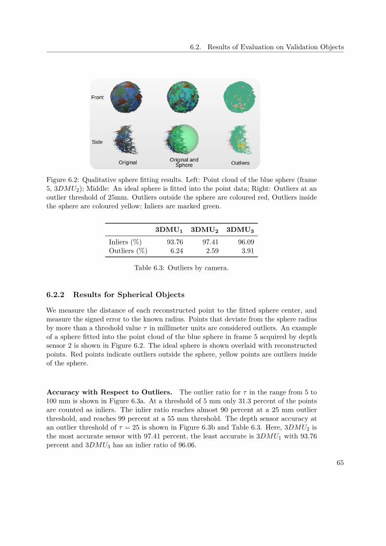
6.2. Results of Evaluation on Validation Objects
Figure 6.2: Qualitative sphere fitting results. Left: Point cloud of the blue sphere (frame5, 3DMU2); Middle: An ideal sphere is fitted into the point data; Right: Outliers at anoutlier threshold of 25mm. Outliers outside the sphere are coloured red, Outliers insidethe sphere are coloured yellow; Inliers are marked green.
3DMU1 3DMU2 3DMU3
Inliers (%) 93.76 97.41 96.09Outliers (%) 6.24 2.59 3.91
Table 6.3: Outliers by camera.
6.2.2 Results for Spherical Objects
We measure the distance of each reconstructed point to the fitted sphere center, andmeasure the signed error to the known radius. Points that deviate from the sphere radiusby more than a threshold value τ in millimeter units are considered outliers. An exampleof a sphere fitted into the point cloud of the blue sphere in frame 5 acquired by depthsensor 2 is shown in Figure 6.2. The ideal sphere is shown overlaid with reconstructedpoints. Red points indicate outliers outside the sphere, yellow points are outliers insideof the sphere.
Accuracy with Respect to Outliers. The outlier ratio for τ in the range from 5 to100 mm is shown in Figure 6.3a. At a threshold of 5 mm only 31.3 percent of the pointsare counted as inliers. The inlier ratio reaches almost 90 percent at a 25 mm outlierthreshold, and reaches 99 percent at a 55 mm threshold. The depth sensor accuracy atan outlier threshold of τ = 25 is shown in Figure 6.3b and Table 6.3. Here, 3DMU2 isthe most accurate sensor with 97.41 percent, the least accurate is 3DMU1 with 93.76percent and 3DMU3 has an inlier ratio of 96.06.
65
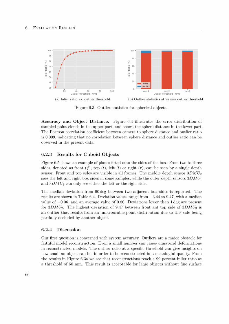
6. Evaluation Results
20 40 60 80 100Outlier Threshold [mm]
30
40
50
60
70
80
90
100
Inlie
r Rat
io [%
]
(a) Inlier ratio vs. outlier threshold
cam 1 cam 2 cam 3Outlier Threshold [mm]
0
20
40
60
80
100
Inlie
r Rat
io [%
]
inliersoutliers
(b) Outlier statistics at 25 mm outlier threshold
Figure 6.3: Outlier statistics for spherical objects.
Accuracy and Object Distance. Figure 6.4 illustrates the error distribution ofsampled point clouds in the upper part, and shows the sphere distance in the lower part.The Pearson correlation coefficient between camera to sphere distance and outlier ratiois 0.009, indicating that no correlation between sphere distance and outlier ratio can beobserved in the present data.
6.2.3 Results for Cuboid Objects
Figure 6.5 shows an example of planes fitted onto the sides of the box. From two to threesides, denoted as front (f), top (t), left (l) or right (r), can be seen by a single depthsensor. Front and top sides are visible in all frames. The middle depth sensor 3DMU2
sees the left and right box sides in some samples, while the outer depth sensors 3DMU1
and 3DMU3 can only see either the left or the right side.
The median deviation from 90 deg between two adjacent box sides is reported. Theresults are shown in Table 6.4. Deviation values range from −3.44 to 9.47, with a medianvalue of −0.06, and an average value of 0.80. Deviations lower than 1 deg are presentfor 3DMU2. The highest deviation of 9.47 between front ant top side of 3DMU3 isan outlier that results from an unfavourable point distribution due to this side beingpartially occluded by another object.
6.2.4 Discussion
Our first question is concerned with system accuracy. Outliers are a major obstacle forfaithful model reconstruction. Even a small number can cause unnatural deformationsin reconstructed models. The outlier ratio at a specific threshold can give insights onhow small an object can be, in order to be reconstructed in a meaningful quality. Fromthe results in Figure 6.3a we see that reconstructions reach a 99 percent inlier ratio ata threshold of 50 mm. This result is acceptable for large objects without fine surface
66

6.2. Results of Evaluation on Validation Objects
150
100
50
0
50
100
150
Sign
ed E
rror [
mm
]
blue
- f4
cam
0
blue
- f4
cam
1
blue
- f4
cam
2
blue
- f3
cam
0
blue
- f3
cam
2
blue
- f3
cam
1
gree
n - f
5 ca
m2
gree
n - f
5 ca
m0
blue
- f0
cam
2
gree
n - f
5 ca
m1
blue
- f2
cam
1
blue
- f2
cam
0
blue
- f2
cam
2
blue
- f1
cam
1
blue
- f1
cam
0
blue
- f1
cam
2
gree
n - f
6 ca
m1
gree
n - f
6 ca
m0
gree
n - f
6 ca
m2
blue
- f5
cam
0
blue
- f5
cam
1
blue
- f5
cam
2
Data set
2900
2800
2700
2600
2500
2400
2300
Dist
ance
to C
amer
a [m
m]
Figure 6.4: Sphere point distribution and distance. Top: Point distribution of spheresamples. A white dot at the bar center of each coloured area denotes the respectivemedian signed error value, the thick black bar within the coloured area denotes upperand lower quartile. The coloured areas indicate the error distribution. Bottom: Distanceof the sphere centre to the camera.
Depth Sensor ∆ft ∆fl ∆tl ∆fr ∆tr
3DMU1 2.44 – – 2.96 -3.443DMU2 2.18 -0.06 -0.14 -0.72 -2.723DMU3 9.47 -2.95 1.83 – –
Table 6.4: Box reconstruction accuracy. Box sides are denoted as front (f), top (t),left (l) and right (r). Rows denote values per depth sensor. Columns 2-6 contain mediandeviations from 90 deg between two adjacent box sides.
67
6. Evaluation Results
Figure 6.5: Illustration of plane fitting for a cuboid object. From left to right: The inputimage shows the box as placed in the scene; Reconstructed point cloud; Point cloud withoverlaid fitted planes and plane normal vectors; Point cloud of the box shown from adifferent viewing angle.
details. To reconstruct smaller objects like a human face, a higher accuracy is needed.In Figure 5.13 in Section 5.1, an example of a person’s face has been presented, wherea chin was enlarged, whereas the nose was flattened. A possible solution to improvethe reconstruction would be to increase the disparity range of the acquired disparitymaps, which can be achieved by either increasing the depth sensor’s stereo baseline orto decrease the object to camera distance. Regarding the accuracy of the depth sensorsresults of the sphere, our evaluation indicates that 3DMU1 is the worst performing.
The second question of this evaluation is on the influence of the object-to-camera distanceon the reconstruction accuracy. In the present data, spheres where placed at distancesfrom approximately 2.3 to 2.9 meters. No correlation at this distance range could beshown.
The evaluation on a cuboid validation object has shown that orthogonal angles of a boxcan be reconstructed to a high accuracy of up to 0.06 deg deviation from orthogonality.Other measurements, on the other hand, show significantly lower accuracy, for whichtwo reasons can be pointed out. First, outliers affect the plane fitting process based onleast squares regression. The second reason has to do with the acquired data set. Insome samples only a low number of plane points represent a side, as they were frequentlyobstructed by other objects.
6.3 Results of Novel View Evaluation
In this section, novel view evaluation results are presented and discussed. The generalprocedure has been laid out in Section 5.2.2. We first discuss the creation and preparationof the data set in Section 6.3.1. Next, results in terms of accuracy for the individualdepth sensors are presented in Section 6.3.2. Then, we look into the results for novel viewaccuracy in Section 6.3.3. Finally, the results are discussed in more depth in Section 6.3.4.
68

6.3. Results of Novel View Evaluation
6.3.1 Data Set
For novel view evaluation, we use the 3D models and approaches variations described inSection 5.2.2. Five different 3D models, and in total six approaches of model generationare examined, which are divided into three point cloud generation, and two view fusionmethods. Point cloud generation methods are denoted as ID for point clouds computedfrom CVF integer-valued disparity maps, DR for point clouds generated from CVFdisparity maps with sub-pixel values and disparity filtering, and PM for point cloudscomputed from a PatchMatch algorithm. The examined fusion methods are view fusionbefore model generation (FB) and view fusion after model generation (FA). In thefollowing, we examine various system products resulting from different processing stages.In particular, pnts-raw denotes original per view point clouds that serve as input tomodel generation. pnts-fa/pnts-fb are smoothed point clouds, created by modelgeneration, and mesh-fa/mesh-fb are coloured meshes created by model generation.Variants with the fb suffix are only available for the novel view 3DMU1+3, as they aregenerated from the two outward views.
6.3.2 Results of Depth Sensors
Completeness Results. Completeness describes the ratio of image pixels subjectto similarity computation to the total number of image pixels. Figure 6.6 shows ourmodel completeness. The average is 5.7 percent in terms of the total input image size.Three factors contribute to this rather low value. First, only a fraction of the originalinput image size is actually used. Image rectification reduces the active image regionfor 3DMU1, 3DMU2 and 3DMU3 to 80.6, 74.1, and 68.8 percent of the original imagearea. Second, during acquisition the sensors were positioned such that a large personwas able to jump, while still staying within the field of view of each camera. Third, aswe examine segmented models, only regions belonging to the persons are counted. Eachselected model can be fit into a bounding box of 1300 × 1300 pixels size.
Depth Sensor Accuracy. We analyse the individual depth sensor accuracies bycomparing single view products against the original, rectified, image as seen by the leftcamera of the respective sensor. The graphs in Figure 6.7 show the mean model accuracyof examined reconstruction products for each of the three depth sensors. Mean accuracyvalues for each view can be seen in Table 6.5. Figure 6.8 shows qualitative accuracyresults.
The accuracy of the middle sensor 3DMU2 is the rated highest with an average score of0.985. Accuracy ratings among models are largely consistent, as the low deviations fromthe mean value show. The second best sensor 3DMU1 has a slightly lower average of0.97 and exhibits higher accuracy deviations. Lastly, 3DMU3 shows the lowest accuracywith a mean score of 0.92. A reason for the lower performance of 3DMU3 can be seen inthe third column of Figure 6.8. Dark regions at the left edge of the persons indicate aglobal offset of the view of 3DMU3, caused by the rigid registration step.
69
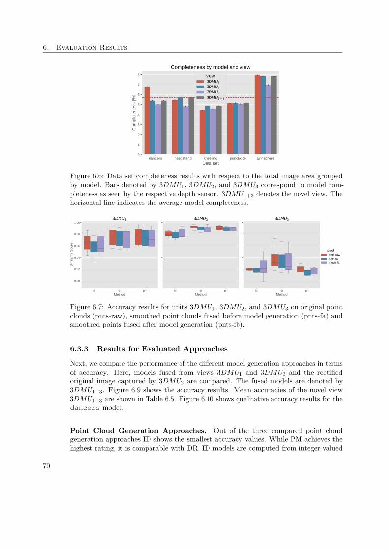
6. Evaluation Results
dancers headstand kneeling punchkick twinsphereData set
0
1
2
3
4
5
6
7
8
Com
plet
enes
s [%
]
Completeness by model and view
view3DMU13DMU23DMU33DMU1+3
Figure 6.6: Data set completeness results with respect to the total image area groupedby model. Bars denoted by 3DMU1, 3DMU2, and 3DMU3 correspond to model com-pleteness as seen by the respective depth sensor. 3DMU1+3 denotes the novel view. Thehorizontal line indicates the average model completeness.
id dr pmMethod
0.90
0.92
0.94
0.96
0.98
1.00
Sim
ilarit
y S
core
3DMU1
id dr pmMethod
3DMU2
id dr pmMethod
3DMU3
prodpntsrawpntsfameshfa
Figure 6.7: Accuracy results for units 3DMU1, 3DMU2, and 3DMU3 on original pointclouds (pnts-raw), smoothed point clouds fused before model generation (pnts-fa) andsmoothed points fused after model generation (pnts-fb).
6.3.3 Results for Evaluated Approaches
Next, we compare the performance of the different model generation approaches in termsof accuracy. Here, models fused from views 3DMU1 and 3DMU3 and the rectifiedoriginal image captured by 3DMU2 are compared. The fused models are denoted by3DMU1+3. Figure 6.9 shows the accuracy results. Mean accuracies of the novel view3DMU1+3 are shown in Table 6.5. Figure 6.10 shows qualitative accuracy results for thedancers model.
Point Cloud Generation Approaches. Out of the three compared point cloudgeneration approaches ID shows the smallest accuracy values. While PM achieves thehighest rating, it is comparable with DR. ID models are computed from integer-valued
70
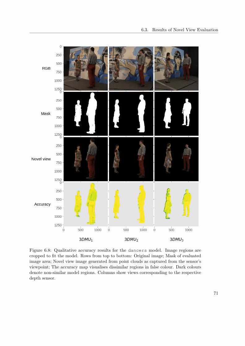
6.3. Results of Novel View Evaluation
Figure 6.8: Qualitative accuracy results for the dancers model. Image regions arecropped to fit the model. Rows from top to bottom: Original image; Mask of evaluatedimage area; Novel view image generated from point clouds as captured from the sensor’sviewpoint; The accuracy map visualises dissimilar regions in false colour. Dark coloursdenote non-similar model regions. Columns show views corresponding to the respectivedepth sensor.
71
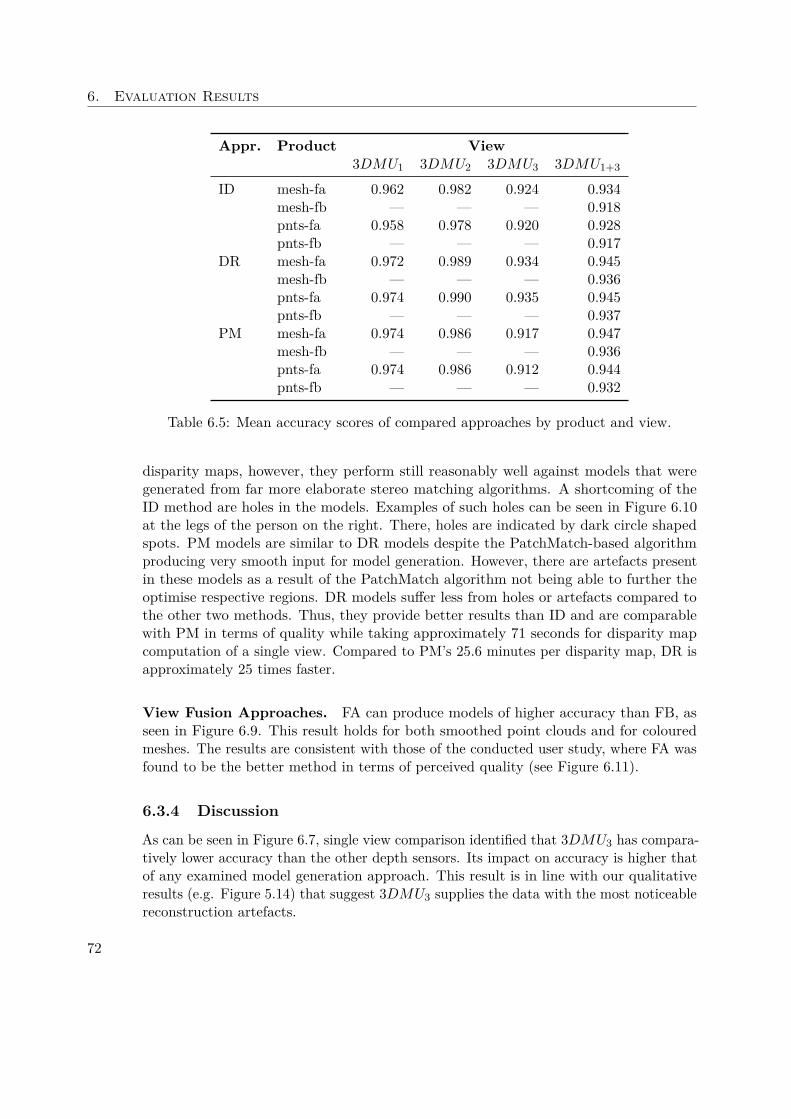
6. Evaluation Results
Appr. Product View3DMU1 3DMU2 3DMU3 3DMU1+3
ID mesh-fa 0.962 0.982 0.924 0.934mesh-fb — — — 0.918pnts-fa 0.958 0.978 0.920 0.928pnts-fb — — — 0.917
DR mesh-fa 0.972 0.989 0.934 0.945mesh-fb — — — 0.936pnts-fa 0.974 0.990 0.935 0.945pnts-fb — — — 0.937
PM mesh-fa 0.974 0.986 0.917 0.947mesh-fb — — — 0.936pnts-fa 0.974 0.986 0.912 0.944pnts-fb — — — 0.932
Table 6.5: Mean accuracy scores of compared approaches by product and view.
disparity maps, however, they perform still reasonably well against models that weregenerated from far more elaborate stereo matching algorithms. A shortcoming of theID method are holes in the models. Examples of such holes can be seen in Figure 6.10at the legs of the person on the right. There, holes are indicated by dark circle shapedspots. PM models are similar to DR models despite the PatchMatch-based algorithmproducing very smooth input for model generation. However, there are artefacts presentin these models as a result of the PatchMatch algorithm not being able to further theoptimise respective regions. DR models suffer less from holes or artefacts compared tothe other two methods. Thus, they provide better results than ID and are comparablewith PM in terms of quality while taking approximately 71 seconds for disparity mapcomputation of a single view. Compared to PM’s 25.6 minutes per disparity map, DR isapproximately 25 times faster.
View Fusion Approaches. FA can produce models of higher accuracy than FB, asseen in Figure 6.9. This result holds for both smoothed point clouds and for colouredmeshes. The results are consistent with those of the conducted user study, where FA wasfound to be the better method in terms of perceived quality (see Figure 6.11).
6.3.4 Discussion
As can be seen in Figure 6.7, single view comparison identified that 3DMU3 has compara-tively lower accuracy than the other depth sensors. Its impact on accuracy is higher thatof any examined model generation approach. This result is in line with our qualitativeresults (e.g. Figure 5.14) that suggest 3DMU3 supplies the data with the most noticeablereconstruction artefacts.
72
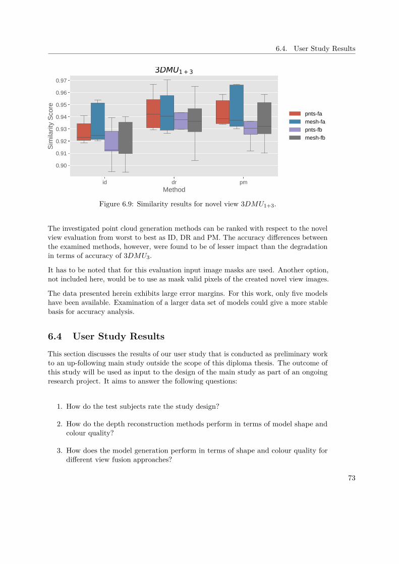
6.4. User Study Results
id dr pmMethod
0.90
0.91
0.92
0.93
0.94
0.95
0.96
0.97
Sim
ilarit
y S
core
3DMU1+3
pntsfameshfapntsfbmeshfb
Figure 6.9: Similarity results for novel view 3DMU1+3.
The investigated point cloud generation methods can be ranked with respect to the novelview evaluation from worst to best as ID, DR and PM. The accuracy differences betweenthe examined methods, however, were found to be of lesser impact than the degradationin terms of accuracy of 3DMU3.
It has to be noted that for this evaluation input image masks are used. Another option,not included here, would be to use as mask valid pixels of the created novel view images.
The data presented herein exhibits large error margins. For this work, only five modelshave been available. Examination of a larger data set of models could give a more stablebasis for accuracy analysis.
6.4 User Study Results
This section discusses the results of our user study that is conducted as preliminary workto an up-following main study outside the scope of this diploma thesis. The outcome ofthis study will be used as input to the design of the main study as part of an ongoingresearch project. It aims to answer the following questions:
1. How do the test subjects rate the study design?
2. How do the depth reconstruction methods perform in terms of model shape andcolour quality?
3. How does the model generation perform in terms of shape and colour quality fordifferent view fusion approaches?
73
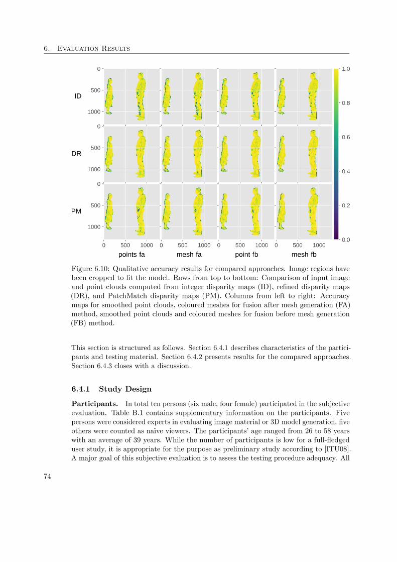
6. Evaluation Results
Figure 6.10: Qualitative accuracy results for compared approaches. Image regions havebeen cropped to fit the model. Rows from top to bottom: Comparison of input imageand point clouds computed from integer disparity maps (ID), refined disparity maps(DR), and PatchMatch disparity maps (PM). Columns from left to right: Accuracymaps for smoothed point clouds, coloured meshes for fusion after mesh generation (FA)method, smoothed point clouds and coloured meshes for fusion before mesh generation(FB) method.
This section is structured as follows. Section 6.4.1 describes characteristics of the partici-pants and testing material. Section 6.4.2 presents results for the compared approaches.Section 6.4.3 closes with a discussion.
6.4.1 Study Design
Participants. In total ten persons (six male, four female) participated in the subjectiveevaluation. Table B.1 contains supplementary information on the participants. Fivepersons were considered experts in evaluating image material or 3D model generation, fiveothers were counted as naïve viewers. The participants’ age ranged from 26 to 58 yearswith an average of 39 years. While the number of participants is low for a full-fledgeduser study, it is appropriate for the purpose as preliminary study according to [ITU08].A major goal of this subjective evaluation is to assess the testing procedure adequacy. All
74
6.4. User Study Results
persons passed the screening procedure comprising a visual acuity and colour vision test,and could perform the subjective evaluation. Additionally, the participants’ opinions werescreened by subsequent statistical processing for biased or incoherent judgements withthe algorithm for determining the transitivity satisfaction rate described in Section 5.2.3.No circular triads were detected, consequently all judgements could be used for statisticalanalysis.
Testing Material. In total six different model generation approaches divided intothree methods of point cloud generation and two view fusion methods where compared.Five acquired 3D models were selected for evaluation. The evaluated approaches and usedmodels have been discussed in Section 6.1. For each model and approach we rendered 20second long videos showing the model as seen from along a camera path that passed fourpredefined positions. Three of positions corresponded to those of 3DMU1, 3DMU2 and3DMU3. An additional novel fourth viewpoint was inserted slightly above the middle3DMU. In pair comparison any approach is compared against all others. Thus, a singlecomparison set consists of 6×5
2 = 15 comparisons. Each comparison set is shown for all 5models, resulting in 5 × 15 = 75 comparisons. The total show time was 75 × 20 = 1500seconds or 25 minutes per person. Participants deemed the evaluation time as challenging,but appropriate.
6.4.2 Compared Approaches
Mean opinion scores were obtained as described in Section 5.2.3 and are shown inFigure 6.11, grouped by model.
Point Cloud Generation Approaches. The subjective evaluation results in a clearpreference for DR, with ID second, and PM last (see Figure 6.11a). Ratings are consistentamong the majority of models, namely “dancers”, “headstand” and “kneeling”. Modelsgenerated with DR exhibit comparatively round surface features, especially in faces.Participants’ comments indicate this fact as the major factor for their preference. IDmodels have more holes than the other methods. Further, faces tend to be rather flat,due to low spatial resolution of the point clouds that serve as input for model generation.While PM models have fewer holes and rounder surface features compared to the othermethods, their quality was perceived as inferior to the others. A reason for this is thelarge artefacts that appear in them. Although observers were instructed to dismiss themwhen performing their judgement, feedback comments indicate that they still had asignificant impact on the given opinions.
View Fusion Approaches. Results of the view fusion evaluation can be seen inFigure 6.11b. Overall, the fusion of single views after model generation (FA) was clearlypreferred by observers over view fusion before model generation (FB). In FA view fusion,no colour interpolation among individual views is performed resulting in visible ridgeswhere views meet, as can be seen in Figure 6.12. On the other hand, colour interpolation
75
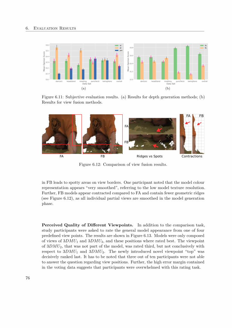
6. Evaluation Results
dancers headstand kneeling punchkick twinsphere overallData Set
0.0
0.1
0.2
0.3
0.4
0.5
0.6M
ean
Opin
ion
Scor
eiddrpm
(a)
dancers headstand kneeling punchkick twinsphere overallData Set
0.0
0.2
0.4
0.6
0.8
Mea
n Op
inio
n Sc
ore
fafb
(b)
Figure 6.11: Subjective evaluation results. (a) Results for depth generation methods; (b)Results for view fusion methods.
FA
FB
Ridges vs SpotsFBFA Contractions
FBFA
Figure 6.12: Comparison of view fusion results.
in FB leads to spotty areas on view borders. One participant noted that the model colourrepresentation appears “very smoothed”, referring to the low model texture resolution.Further, FB models appear contracted compared to FA and contain fewer geometric ridges(see Figure 6.12), as all individual partial views are smoothed in the model generationphase.
Perceived Quality of Different Viewpoints. In addition to the comparison task,study participants were asked to rate the general model appearance from one of fourpredefined view points. The results are shown in Figure 6.13. Models were only composedof views of 3DMU1 and 3DMU3, and these positions where rated best. The viewpointof 3DMU2, that was not part of the model, was rated third, but not conclusively withrespect to 3DMU1 and 3DMU3. The newly introduced novel viewpoint “top” wasdecisively ranked last. It has to be noted that three out of ten participants were not ableto answer the question regarding view positions. Further, the high error margin containedin the voting data suggests that participants were overwhelmed with this rating task.
76

6.4. User Study Results
3DMU1 3DMU2 Top 3DMU30
1
2
3
4
5
Ratin
g
Figure 6.13: Subjective ratings of view point positions.
6.4.3 Discussion
Regarding the questions asked in this study, the following conclusions can be drawn.Overall, the study design was perceived as suitable by the observers. 25 minutes of modelshow time was adequate, but should not be increased further. Voting was performedon a separate dark screen showing only buttons for the judgement according to therecommendation of [ITU08]. Multiple participants reported difficulty of identifyingvideos A and B, as they could not see the models on the voting screen any more. Thesituation could be improved by showing both models while the viewer votes. Showingmodels from different perspectives was appreciated. The position rating task, however,was too much to ask. Three observers noted that the last position was the most dominantin their memory. This suggests, that the viewpoint order of the camera path can biasthe position-rating task.
All participants noted geometric issues on models, especially the faces were of concern.Fusion of the models from two far apart views leads to faces being duplicated or outrightmissing. Single view meshes of ID models are to “flat” to achieve an accurate reconstruc-tion of features, further they have too many holes due to locally too sparse point datafor the model generation. Both the DR and PM methods can reproduce round features,like heads, to a better degree, but ultimately also struggle in accurate reconstruction.PM generated models exhibited large free-floating artefacts that are especially visiblewhen showing models from view points other than the capturing sensor.
In the FB method, persons faces tend to disappear in the meshes due to smoothingapplied in the model generation phase and the relatively low overlap between the fusedviews. With the available data, no model was convincingly reproduced. Geometricbodies had noticeable shape distortions that can be traced to outlier points present inthe original point clouds, and aggressive smoothing applied for model generation. Simplecolour interpolation can reproduce texture from RGB images only with limited quality.Other available methods, such as [EFR+17, DCC+18], need be to used to recover modeltexture more accurately.
77

CHAPTER 7Conclusion
In this thesis, we have presented an evaluation framework for assessing the qualityof point clouds and textured meshes acquired by a 3D reconstruction system thatcomprises multiple stereo sensors. Our evaluation determines two important propertiesof reconstructed 3D models: (i) the geometric fidelity of reconstructed objects, and (ii)the subjective model quality perceived by the user.
After providing some background information and a literature review on 3D recon-struction and related evaluation methodologies, we presented our proposed evaluationframework along with selected aspects of its implementation. An important part ofour study demonstrates the application of our implemented evaluation modules on a3D reconstruction system that obtains textured mesh models of dynamic scenes withthree stereo cameras. One of the goals of our evaluation was to compare the qualityachieved by different stereo matching and 3D model merging algorithms included inthe examined multi-view stereo system. To this end, a set of intermediate and finalsystem products were examined using three complementary quantitative and qualitativeevaluation strategies. First, an evaluation with geometrically simple validation objects(sphere, cuboid) of known dimensions determined the geometric reconstruction qualityby comparing object reconstructions against ideal models by means of shape fitting.The results of this evaluation were used to determine the geometric accuracy of pointclouds obtained with the system in terms of reconstructed shape, size and angles betweenplanar surfaces. The results show that the examined 3D imaging system is capable ofreconstructing spherical point clouds with 90 percent accuracy at an outlier thresholdof 25 mm and angles between adjacent faces of cuboid objects with a deviation of aslow as 0.06 degree. Second, a quantitative image-based novel view evaluation assessedthe quality of the acquired point clouds and textured mesh models in terms of imagesimilarity. More precisely, we found that the examined CVF and PatchMatch stereocorrespondence algorithms delivered comparable results in terms of textured mesh model
79
7. Conclusion
accuracy, when their output was used to generate mesh models, while CVF was fasterthan PatchMatch by a factor of 25.
Third, a subjective user study determined the perceived quality of textured mesh modelsof several depth reconstruction approaches. We also observed that the subjective rankingswere inconsistent with those determined by our novel view evaluation, which confirms theneed for a combined approach of quantitative and qualitative evaluation. In this contextwe noticed some model imperfections localized in small areas close to object boundariesthat influenced the image-based similarity results only by a small amount, while thesame imperfections dominated the subjective appearance, when shown in a 3D view ofthe scene.
The present evaluation methodology assumed reasonably accurate stereo sensor calibra-tion. A possible topic for future work would be to include the effects of non-perfectsensor calibration into the analysis of our 3D reconstruction system. Furthermore, theincorporation of quality aspects that are specific to dynamic scenes (for example, tomeasure flickering artefacts) would be a valuable future extension.
80
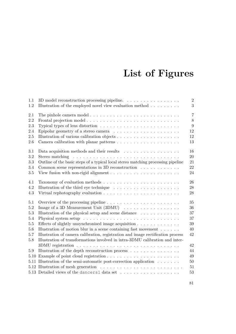
List of Figures
1.1 3D model reconstruction processing pipeline. . . . . . . . . . . . . . . . . 21.2 Illustration of the employed novel view evaluation method . . . . . . . . . 3
2.1 The pinhole camera model . . . . . . . . . . . . . . . . . . . . . . . . . . . 72.2 Frontal projection model . . . . . . . . . . . . . . . . . . . . . . . . . . . . 82.3 Typical types of lens distortion . . . . . . . . . . . . . . . . . . . . . . . . 92.4 Epipolar geometry of a stereo camera . . . . . . . . . . . . . . . . . . . . 122.5 Illustration of various calibration objects . . . . . . . . . . . . . . . . . . . 122.6 Camera calibration with planar patterns . . . . . . . . . . . . . . . . . . . 13
3.1 Data acquisition methods and their results . . . . . . . . . . . . . . . . . 163.2 Stereo matching . . . . . . . . . . . . . . . . . . . . . . . . . . . . . . . . 203.3 Outline of the basic steps of a typical local stereo matching processing pipeline 213.4 Common scene representations in 3D reconstruction . . . . . . . . . . . . 223.5 View fusion with non-rigid alignment . . . . . . . . . . . . . . . . . . . . . 24
4.1 Taxonomy of evaluation methods . . . . . . . . . . . . . . . . . . . . . . . 264.2 Illustration of the third eye technique . . . . . . . . . . . . . . . . . . . . 284.3 Virtual rephotography evaluation . . . . . . . . . . . . . . . . . . . . . . . 28
5.1 Overview of the processing pipeline . . . . . . . . . . . . . . . . . . . . . . 355.2 Image of a 3D Measurement Unit (3DMU) . . . . . . . . . . . . . . . . . 365.3 Illustration of the physical setup and scene distance . . . . . . . . . . . . 375.4 Physical system setup . . . . . . . . . . . . . . . . . . . . . . . . . . . . . 375.5 Effects of slightly unsynchronised image acquisition . . . . . . . . . . . . . 395.6 Illustration of motion blur in a scene containing fast movement . . . . . . 405.7 Illustration of camera calibration, registration and image rectification process 425.8 Illustration of transformations involved in intra-3DMU calibration and inter-
3DMU registration . . . . . . . . . . . . . . . . . . . . . . . . . . . . . . . 425.9 Illustration of the depth reconstruction process . . . . . . . . . . . . . . . 445.10 Example of point cloud registration . . . . . . . . . . . . . . . . . . . . . . 495.11 Illustration of the semi-automatic post-correction application . . . . . . . 505.12 Illustration of mesh generation . . . . . . . . . . . . . . . . . . . . . . . . . 515.13 Detailed views of the dancers1 data set . . . . . . . . . . . . . . . . . . 53
81
5.14 Illustration of model artefacts introduced by views . . . . . . . . . . . . . 535.15 Illustration of the lab environment for subjective evaluation . . . . . . . . 575.16 Illustration of the pair-based comparison scheme . . . . . . . . . . . . . . 59
6.1 Models used for novel view evaluation and user study . . . . . . . . . . . 626.2 Qualitative sphere fitting results . . . . . . . . . . . . . . . . . . . . . . . 656.3 Outlier statistics for spherical objects . . . . . . . . . . . . . . . . . . . . 666.4 Sphere point distribution and distance . . . . . . . . . . . . . . . . . . . . 676.5 Illustration of plane fitting for a cuboid object . . . . . . . . . . . . . . . 686.6 Data set completeness results . . . . . . . . . . . . . . . . . . . . . . . . . 706.7 Accuracy results for units 3DMU1, 3DMU2, and 3DMU3 . . . . . . . . . 706.8 Qualitative accuracy results for the dancers model . . . . . . . . . . . . . 716.9 Similarity results for novel view 3DMU1+3 . . . . . . . . . . . . . . . . . 736.10 Qualitative accuracy results for compared approaches . . . . . . . . . . . 746.11 Subjective evaluation results . . . . . . . . . . . . . . . . . . . . . . . . . 766.12 Comparison of view fusion results . . . . . . . . . . . . . . . . . . . . . . . 766.13 Subjective ratings of view point positions . . . . . . . . . . . . . . . . . . 77
B.1 User study instructions in English language . . . . . . . . . . . . . . . . . 100B.2 User study instructions in German language . . . . . . . . . . . . . . . . . . 101B.3 Questionnaire page 1 . . . . . . . . . . . . . . . . . . . . . . . . . . . . . . 102B.4 Questionnaire page 2 . . . . . . . . . . . . . . . . . . . . . . . . . . . . . . 103B.5 Snellen chart . . . . . . . . . . . . . . . . . . . . . . . . . . . . . . . . . . 104B.6 Pseudoisochromatic plates . . . . . . . . . . . . . . . . . . . . . . . . . . . 105
82

List of Tables
4.1 Viewing conditions for subjective assessment . . . . . . . . . . . . . . . . 30
5.1 System hardware characteristics . . . . . . . . . . . . . . . . . . . . . . . 365.2 Stereo matching parameters . . . . . . . . . . . . . . . . . . . . . . . . . . 45
6.1 Products used for novel-view evaluation and the user study . . . . . . . . . 616.2 Evaluated approaches for novel view evaluation and user study . . . . . . 646.3 Outliers by camera . . . . . . . . . . . . . . . . . . . . . . . . . . . . . . . 656.4 Box reconstruction accuracy . . . . . . . . . . . . . . . . . . . . . . . . . . 676.5 Mean accuracy scores of compared approaches by product and view . . . 72
A.1 Ground truth measurements taken of cameras, objects and scene features 98
B.1 Detailed information on participants of the user study. . . . . . . . . . . . 106
83

Acronyms
2D Two-dimensional 6
3D Three-dimensional 1
3DMU 3D Measurement Unit 34, 36
ACR Absolute Category Rating 31
APSS Algebraic Point Set Surfaces 49
CVF Cost Volume Filtering 62, 79
DSQS Double Stimulus Continuous Quality-Scale 31
FPS Frames Per Second 38
ITU International Telecommunication Union 29
NCC Normalized Cross Correlation 18, 56
PC Pair-based Comparison 31
RGB Red, Green, Blue 16
RGB-D Red, Green, Blue plus Depth 16
SAD Sum of Absolute Differences 17
TOF Time-Of-Flight 16
WTA Winner-Takes-All 21, 45
85

Bibliography
[AUE17] Evangelos Alexiou, Evgeniy Upenik, and Touradj Ebrahimi. Towardssubjective quality assessment of point cloud imaging in augmented reality.In IEEE International Workshop on Multimedia Signal Processing, pages1–6, 2017.
[BÁBB+18] Miguel Barreda-Ángeles, Federica Battisti, Giulia Boato, Marco Carli, EmilDumic, Margrit Gelautz, Chaminda Hewage, Dragan Kukolj, Patrick Le-Callet, Antonio Liotta, Cecilia Pasquini, Alexandre Pereda-Baños, ChristosPolitis, Dragana Sandic, Murat Tekalp, María Torres-Vega, and VladimirZlokolica. Quality of experience and quality of service metrics for 3Dcontent. In P. Assunção and A. Gotchev, editors, 3D Visual ContentCreation, Coding and Delivery, pages 267–297. Springer, Cham, 2018.
[BB13] Michael Bleyer and Christian Breiteneder. Stereo Matching - State-of-the-Art and Research Challenges, pages 143–179. Springer London, 2013.
[BKB08] Gary Bradski, Adrian Kaehler, and Gary Bradski. Learning OpenCV -Computer Vision with the OpenCV Library. O’Reilly Media, 2008.
[BKH10] Abdelkrim Belhaoua, Sophie Kohler, and Ernest Hirsch. Error evaluationin a stereovision-based 3D reconstruction system. EURASIP Journal onImage and Video Processing, 2010(1):Article ID 539836, 12 pages, 2010.
[BR15] Libor Bolecek and Vaclav Ricny. Influence of stereoscopic camera systemalignment error on the accuracy of 3D reconstruction. Radioengineering,24(2):610–620, 2015.
[Bra00] G. Bradski. The OpenCV library. Dr. Dobb’s Journal of Software Tools,2000.
[Bro66] Duane C. Brown. Decentering distortion of lenses. Photometric Engineering,32(3):444–462, 1966.
[Bro16] Nicole Brosch. Spatio-temporal Video Analysis for Semi-automatic 2D-to-3D Conversion by. PhD thesis, Vienna University of Technology, 2016.
87
[BRR11] Michael Bleyer, Christoph Rhemann, and Carsten Rother. PatchMatchstereo - stereo matching with slanted support windows. In Proceedings ofthe British Machine Vision Conference, pages 14.1–14.11, 2011.
[BT52] Ralph Allan Bradley and Milton E. Terry. Rank analysis of incomplete blockdesigns: I. The method of paired comparisons. Biometrika, 39(3/4):324,1952.
[BT99] Stan Birchfield and Carlo Tomasi. Depth discontinuities by pixel-to-pixelstereo. International Journal of Computer Vision, 35(3):269–293, 1999.
[BTV06] Herbert Bay, Tinne Tuytelaars, and Luc Van Gool. SURF: Speeded uprobust features. In European Conference on Computer Vision, pages 404–417, 2006.
[CCS+15] Alvaro Collet, Ming Chuang, Pat Sweeney, Don Gillett, Dennis Evseev,David Calabrese, Hugues Hoppe, Adam Kirk, and Steve Sullivan. High-quality streamable free-viewpoint video. ACM Transactions on Graphics,34(4):69:1–69:13, 2015.
[CGEB07] Massimiliano Corsini, Elisa D. Gelasca, Touradj Ebrahimi, and MauroBarni. Watermarked 3-D mesh quality assessment. IEEE Transactions onMultimedia, 9(2):247–255, 2007.
[CGK14] Hsiang-Jen Chien, Haokun Geng, and Reinhard Klette. Improved visualodometry based on transitivity error in disparity space: A third-eye ap-proach. In International Conference on Image and Vision Computing NewZealand, pages 72–77, 2014.
[ÇığlaAA12] Cevahir Çığla and A. Aydın Alatan. An improved stereo matching algorithmwith ground plane and temporal smoothness constraints. In EuropeanConference on Computer Vision. Workshops and Demonstrations, pages134–147, 2012.
[ÇığlaAA13] Cevahir Çığla and A. Aydın Alatan. Information permeability for stereomatching. Signal Processing: Image Communication, 28(9):1072–1088,2013.
[CL96] Brian Curless and Marc Levoy. A volumetric method for building complexmodels from range images. In ACM Conference on Computer graphics andinteractive techniques, pages 303–312, 1996.
[CTF12] Ivan Cabezas, Maria Trujillo, and Margaret Florian. An evaluation method-ology for stereo correspondence algorithms. In International Conferenceon Computer Vision Theory and Applications, pages 154–163, 2012.
88

[Dah] Jeff Dahl. Typical snellen chart to estimate visual acuity. https://
commons.wikimedia.org/wiki/File:Snellen_chart.svg. Ac-cessed: 2018-07-31.
[DCC+18] Ruofei Du, Ming Chuang, Wayne Chang, Hugues Hoppe, and AmitabhVarshney. Montage4D: Interactive seamless fusion of multiview videotextures. In ACM SIGGRAPH Symposium on Interactive 3D Graphicsand Games, pages 1–11, 2018.
[DKK09] Ankur Datta, Jun-Sik Kim, and Takeo Kanade. Accurate camera calibrationusing iterative refinement of control points. In International Conferenceon Computer Vision Workshops, pages 1201–1208, 2009.
[DTK+16] Mingsong Dou, Jonathan Taylor, Pushmeet Kohli, Vladimir Tankovich,et al. Fusion4D: Real-time performance capture of challenging scenes. ACMTransactions on Graphics, 35(4):114:1–114:13, 2016.
[DZC+18] Alexandros Doumanoglou, Nikolaos Zioulis, Emmanouil Christakis, Dim-itrios Zarpalas, and Petros Daras. Subjective quality assessment of texturedhuman full-body 3D-reconstructions. In International Conference on Qual-ity of Multimedia Experience, pages 1–6, 2018.
[EA14] Evan-Amos. Xbox One Kinect Sensor. https://en.wikipedia.org/wiki/File:Microsoft-Xbox-One-Console-Set-wKinect.jpg,2014. Accessed: 2018-07-31.
[EFR+17] Thomas Ebner, Ingo Feldmann, Sylvain Renault, Oliver Schreer, and PeterEisert. Multi-view reconstruction of dynamic real-world objects and theirintegration in augmented and virtual reality applications. Journal of theSociety for Information Display, 25(3):151–157, 2017.
[EXR] EXR file format. Retrieved from https://www.openexr.com/. Ac-cessed: 2018-05-13.
[FBC+18] Karel Fliegel, Federica Battisti, Marco Carli, Margrit Gelautz, LukášKrasula, Patrick Le Callet, and Vladimir Zlokolica. 3D Visual ContentDatasets. In P. Assunção and A. Gotchev, editors, 3D Visual ContentCreation, Coding and Delivery, pages 299–325. Springer, Cham, 2018.
[FH06] Pedro F. Felzenszwalb and Daniel P. Huttenlocher. Efficient belief propaga-tion for early vision. International Journal of Computer Vision, 70(1):41–54,2006.
[FH15] Yasutaka Furukawa and Carlos Hernández. Multi-view stereo: A tutorial.Foundations and Trends in Computer Graphics and Vision, 9(1-2):1–148,2015.
89

[GG07] Gaël Guennebaud and Markus Gross. Algebraic point set surfaces. ACMTransactions on Graphics, 26(3):23, 2007.
[GLU12] A. Geiger, P. Lenz, and R. Urtasun. Are we ready for autonomous driving?The KITTI vision benchmark suite. In IEEE Conference on ComputerVision and Pattern Recognition, pages 3354–3361, 2012.
[GVC+16] Jinjiang Guo, Vincent Vidal, Irene Cheng, Anup Basu, Atilla Baskurt, andGuillaume Lavoue. Subjective and objective visual quality assessment oftextured 3D meshes. ACM Transactions on Applied Perception, 14(2):1–20,2016.
[HBG13] Asmaa Hosni, Michael Bleyer, and Margrit Gelautz. Secrets of adaptivesupport weight techniques for local stereo matching. Computer Vision andImage Understanding, 117(6):620–632, 2013.
[HLCH12] Miles Hansard, Seungkyu Lee, Ouk Choi, and Radu Horaud. Time-of-FlightCameras: Principles, Methods and Applications. Springer, 2012.
[HM12] Xiaoyan Hu and Philippos Mordohai. A quantitative evaluation of confi-dence measures for stereo vision. IEEE Transactions on Pattern Analysisand Machine Intelligence, 34(11):2121–2133, 2012.
[HRB+13] Asmaa Hosni, Christoph Rhemann, Michael Bleyer, Carsten Rother, andMargrit Gelautz. Fast cost-volume filtering for visual correspondence andbeyond. IEEE Transactions on Pattern Analysis and Machine Intelligence,35(2):504–511, 2013.
[HS07] Heiko Hirschmüller and Daniel Scharstein. Evaluation of cost functions forstereo matching. In IEEE Conference on Computer Vision and PatternRecognition, pages 1–8, 2007.
[HZ04] Richard Hartley and Andrew Zisserman. Multiple View Geometry inComputer Vision. Cambridge University Press, second edition, 2004.
[Ish] Pseudoisochomatic plate color vision test. http://www.
colorvisiontesting.com/ishihara. Accessed: 2018-07-31.
[ITU08] ITU. Recommendation ITU-R P.910: Subjective video quality assessmentmethods for multimedia applications, 2008.
[ITU12] ITU. Recommendation ITU-R BT.500: Methodology for the subjectiveassessment of the quality of television pictures, 2012.
[KH13] Michael Kazhdan and Hugues Hoppe. Screened poisson surface reconstruc-tion. ACM Transactions on Graphics, 32(3):1–13, 2013.
90

[KHSM17] Andreas Kuhn, Heiko Hirschmüller, Daniel Scharstein, and Helmut Mayer.A TV prior for high-quality scalable multi-view stereo reconstruction.International Journal of Computer Vision, 124(1):2–17, 2017.
[KIT] The KITTI Vision Benchmark Suite. http://www.cvlibs.net/
datasets/kitti/. Accessed: 2018-04-06.
[Kle14] Reinhard Klette. Concise Computer Vision. Springer London, 2014.
[LC87] William E. Lorensen and Harvey E. Cline. Marching cubes: A highresolution 3D surface construction algorithm. In Computer graphics andinteractive techniques, pages 163–169, 1987.
[LGE13] Jong Seok Lee, Lutz Goldmann, and Touradj Ebrahimi. Paired comparison-based subjective quality assessment of stereoscopic images. MultimediaTools and Applications, 67(1):31–48, 2013.
[LHKP13] Bo Li, Lionel Heng, Kevin Koser, and Marc Pollefeys. A multiple-camerasystem calibration toolbox using a feature descriptor-based calibrationpattern. In IEEE International Conference on Intelligent Robots andSystems, pages 1301–1307, 2013.
[LNSW16] Minglei Li, Liangliang Nan, Neil Smith, and Peter Wonka. Reconstructingbuilding mass models from UAV images. Computers and Graphics, 54:84–93,2016.
[Low04] David G Lowe. Distinctive image features from scale-invariant keypoints.International Journal of Computer Vision, 60(2):91–110, 2004.
[LZYZ18] Lincheng Li, Shunli Zhang, Xin Yu, and Li Zhang. PMSC: PatchMatch-based superpixel cut for accurate stereo matching. IEEE Transactions onCircuits and Systems for Video Technology, 28(3):679–692, 2018.
[MAM14] Nicolas Mellado, Dror Aiger, and Niloy J. Mitra. Super 4PCS fast globalpointcloud registration via smart indexing. Computer Graphics Forum,33(5):205–215, 2014.
[MHW+13] Ziyang Ma, Kaiming He, Yichen Wei, Jian Sun, and Enhua Wu. Constanttime weighted median filtering for stereo matching and beyond. In IEEEInternational Conference on Computer Vision, pages 49–56, 2013.
[Mida] Middlebury Multi-View Stereo - Online Evaluation. http://vision.
middlebury.edu/mview/eval/. Accessed: 2018-04-18.
[Midb] Middlebury Stereo - Online Evaluation. http://vision.middlebury.edu/stereo/. Accessed: 2018-04-18.
91
[MK09] Sandino Morales and Reinhard Klette. A third eye for performance evalua-tion in stereo sequence analysis. In International Conference on ComputerAnalysis of Images and Patterns, pages 1078–1086, 2009.
[Mon07] David Monniaux. Leica terrestrial lidar scanner. https://commons.
wikimedia.org/wiki/File:Lidar_P1270901.jpg, 2007. Ac-cessed: 2018-07-31.
[NBG13] Matej Nezveda, Nicole Brosch, and Margrit Gelautz. Hyperion 3D -intelligent workflow design for low-cost 3D film production working package4. Technical report, Vienna University of Technology, 2013.
[NBSG14] Matej Nezveda, Nicole Brosch, Florian Seitner, and Margrit Gelautz. Depthmap post-processing for depth-image-based rendering: a user study. InSPIE 9011, Stereoscopic Displays and Applications XXV, page 90110K,2014.
[Nez14] Matej Nezveda. Evaluation of depth map post-processing techniques fornovel view generation. Master’s thesis, Vienna University of Technology,2014.
[Nym17] Bengt Nyman. Digital single-lens reflex camera - NikonD810. https://commons.wikimedia.org/wiki/File:
Nikon_D810_EM1B6357-2.jpg, 2017. Accessed: 2018-07-31.
[OEDT+16] Sergio Orts-Escolano, Mingsong Dou, Vladimir Tankovich, Charles Loop,Qin Cai, Philip A. Chou, Sarah Mennicken, Julien Valentin, Vivek Pradeep,Shenlong Wang, Sing Bing Kang, Christoph Rhemann, Pushmeet Kohli,Yuliya Lutchyn, Cem Keskin, Shahram Izadi, Sean Fanello, Wayne Chang,Adarsh Kowdle, Yury Degtyarev, David Kim, Philip L. Davidson, andSameh Khamis. Holoportation: Vitual 3D teleportation in real-time. InSymposium on User Interface Software and Technology, pages 741–754,2016.
[PLY] PLY-polygon file format. Retrieved from http://paulbourke.net/
dataformats/ply/. Accessed: 2018-05-13.
[SAB+07] Elena Stoykova, A. Aydin Alatan, Philip Benzie, Nikos Grammalidis, SourisMalassiotis, Joern Ostermann, Sergej Piekh, Ventseslav Sainov, ChristianTheobalt, Thangavel Thevar, and Xenophon Zabulis. 3-D time-varyingscene capture technologies - a survey. IEEE Transactions on Circuits andSystems for Video Technology, 17(11):1568–1586, 2007.
[SBMM15] Aaron N Staranowicz, Garrett R Brown, Fabio Morbidi, and Gian-LucaMariottini. Practical and accurate calibration of RGB-D cameras usingspheres. Computer Vision and Image Understanding, 137:102–114, 2015.
92
[SCD+06] S.M. Seitz, Brian Curless, James Diebel, Daniel Scharstein, and RichardSzeliski. A comparison and evaluation of multi-view stereo reconstruc-tion algorithms. In IEEE Conference on Computer Vision and PatternRecognition, volume 1, pages 519–528, 2006.
[SCK15] Bok Suk Shin, Diego Caudillo, and Reinhard Klette. Evaluation of twostereo matchers on long real-world video sequences. Pattern Recognition,48(4):1109–1120, 2015.
[SCSK13] Verónica Suaste, Diego Caudillo, Bok-Suk Shin, and Reinhard Klette. Third-eye stereo analysis evaluation enhanced by data measures. In MexicanConference on Pattern Recognition, pages 74–83, 2013.
[Sha98] C.M. Shakarji. Least-squares fitting algorithms of the NIST algorithmtesting system. Journal of Research of the National Institute of Standardsand Technology, 103(6):633, 1998.
[SHK+14] Daniel Scharstein, Heiko Hirschmüller, York Kitajima, Greg Krathwohl,Nera Nešić, Xi Wang, and Porter Westling. High-resolution stereo datasetswith subpixel-accurate ground truth. In Pattern Recognition, volume 8753,pages 31–42, 2014.
[SLK15] Hamed Sarbolandi, Damien Lefloch, and Andreas Kolb. Kinect rangesensing: Structured-light versus Time-of-Flight Kinect. Computer Visionand Image Understanding, 139:1–20, 2015.
[SMP05] Tomáš Svoboda, Daniel Martinec, and Tomáš Pajdla. A convenient multi-camera self-calibration for virtual environments. Presence: Teleoperatorsand Virtual Environments, 14(4):407–422, 2005.
[SNG+15] Florian Seitner, Matej Nezveda, Margrit Gelautz, Georg Braun, ChristianKapeller, Werner Zellinger, and Bernhard Moser. Trifocal system for high-quality inter-camera mapping and virtual view synthesis. In InternationalConference on 3D Imaging, pages 1–8, 2015.
[SS02] Daniel Scharstein and Richard Szeliski. A taxonomy and evaluation ofdense two-frame stereo correspondence algorithms. International Journalof Computer Vision, 47(1-3):7–42, 2002.
[SS03] Daniel Scharstein and Richard Szeliski. High-accuracy stereo depth mapsusing structured light. In IEEE Conference on Computer Vision andPattern Recognition, volume 1, pages 195–202, 2003.
[SSG+17] Thomas Schöps, Johannes L. Schönberger, Silvano Galliani, Torsten Sattler,Konrad Schindler, Marc Pollefeys, and Andreas Geiger. A multi-view stereobenchmark with high-resolution images and multi-camera videos. In IEEEConference on Computer Vision and Pattern Recognition, pages 2538–2547,2017.
93
[SSP07] Robert W Sumner, Johannes Schmid, and Mark Pauly. Embedded defor-mation for shape manipulation. ACM Transactions on Graphics, 26(3):80,2007.
[Sze99] Richard Szeliski. Prediction error as a quality metric for motion and stereo.In IEEE International Conference on Computer Vision, pages 781–788,1999.
[TWC15] Fakhri Torkhani, Kai Wang, and Jean-Marc Chassery. Perceptual qualityassessment of 3D dynamic meshes: Subjective and objective studies. SignalProcessing: Image Communication, 31:185–204, 2015.
[VCB15] Camilo Vargas, Ivan Cabezas, and John W Branch. Stereo correspondenceevaluation methods: A systematic review. In Advances in Visual Computing,pages 102–111, 2015.
[VSKL17] K. Vanhoey, B. Sauvage, P. Kraemer, and G. Lavoué. Visual qualityassessment of 3D models: On the influence of light-material interaction.ACM Transactions on Applied Perception, 15(1), 2017.
[VV14] Patrick Vandewalle and Chris Varekamp. Disparity map quality for image-based rendering based on multiple metrics. In International Conference on3D Imaging, pages 1–5, 2014.
[WBF+17] Michael Waechter, Mate Beljan, Simon Fuhrmann, Nils Moehrle, JohannesKopf, and Michael Goesele. Virtual rephotography. ACM Transactions onGraphics, 36(1):1–11, 2017.
[WFR+16] Shenlong Wang, Sean Ryan Fanello, Christoph Rhemann, Shahram Izadi,and Pushmeet Kohli. The Global Patch Collider. In IEEE Conference onComputer Vision and Pattern Recognition, pages 127–135, 2016.
[WKZ+16] Katja Wolff, Changil Kim, Henning Zimmer, Christopher Schroers, MarioBotsch, Olga Sorkine-Hornung, and Alexander Sorkine-Hornung. Pointcloud noise and outlier removal for image-based 3D reconstruction. InInternational Conference on 3D Vision, pages 118–127, 2016.
[XIM] XIMEA GmbH. Ximea MC050CG-SY product specification brochure.https://www.ximea.com/files/brochures/xiC-USB3_1-
Sony-CMOS-Pregius-cameras-brochure-HQ.pdf. Accessed:2018-02-18.
[YGX+17] Tao Yu, Kaiwen Guo, Feng Xu, Yuan Dong, Zhaoqi Su, Jianhui Zhao,Jianguo Li, Qionghai Dai, and Yebin Liu. BodyFusion: Real-time captureof human motion and surface geometry using a single depth camera. IEEEInternational Conference on Computer Vision, pages 910–919, 2017.
94
[YYDN07] Qingxiong Yang, Ruigang Yang, James Davis, and David Nister. Spatial-depth super resolution for range images. In IEEE Conference on ComputerVision and Pattern Recognition, pages 1–8, 2007.
[Zah85] Johann Zahn. Oculus artificialis teledioptricus sive Telescopium, ex abditisrerum naturalium & artificialium principiis protractum nova methodo,eaque solida explicatum ac comprimis e triplici fundamento physico seunaturali, mathematico dioptrico et mechanico, seu practico stabilitum. Nopublisher, 1685.
[ZFM+17] Kang Zhang, Yuqiang Fang, Dongbo Min, Lifeng Sun, Shiqiang Yang, andShuicheng Yan. Cross-scale cost aggregation for stereo matching. IEEETransactions on Circuits and Systems for Video Technology, 27(5):965–976,2017.
[Zha00] Zhengyou Zhang. A flexible new technique for camera calibration. IEEETransactions on Pattern Analysis and Machine Intelligence, 22(11):1330–1334, 2000.
[Zha04] Zhengyou Zhang. Camera calibration with one-dimensional objects. IEEETransactions on Pattern Analysis and Machine Intelligence, 26(7):892–899,2004.
[ZSG+18] Michael Zollhöfer, Patrick Stotko, Andreas Görlitz, Christian Theobalt,Matthias Nießner, Reinhard Klein, and Andreas Kolb. State of the arton 3D reconstruction with RGB-D cameras. Computer Graphics Forum,37(2):625–652, 2018.
[ZTDVAL14] P. J. Zarco-Tejada, R. Diaz-Varela, V. Angileri, and P. Loudjani. Treeheight quantification using very high resolution imagery acquired from anunmanned aerial vehicle (UAV) and automatic 3D photo-reconstructionmethods. European Journal of Agronomy, 55:89–99, 2014.
[ZW94] Ramin Zabih and John Woodfill. Non-parametric local transforms forcomputing visual correspondence. In European Conference on ComputerVision, pages 151–158, 1994.
95


Appendix A - System Ground
Truth Measurements
Table A.1 lists ground truth measurements that where taken of cameras, prominent scenefeatures, and objects.
97
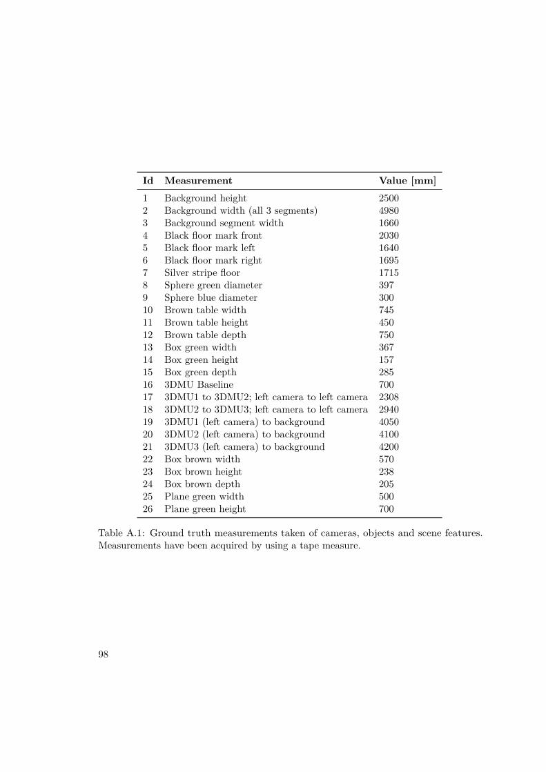
Id Measurement Value [mm]
1 Background height 25002 Background width (all 3 segments) 49803 Background segment width 16604 Black floor mark front 20305 Black floor mark left 16406 Black floor mark right 16957 Silver stripe floor 17158 Sphere green diameter 3979 Sphere blue diameter 30010 Brown table width 74511 Brown table height 45012 Brown table depth 75013 Box green width 36714 Box green height 15715 Box green depth 28516 3DMU Baseline 70017 3DMU1 to 3DMU2; left camera to left camera 230818 3DMU2 to 3DMU3; left camera to left camera 294019 3DMU1 (left camera) to background 405020 3DMU2 (left camera) to background 410021 3DMU3 (left camera) to background 420022 Box brown width 57023 Box brown height 23824 Box brown depth 20525 Plane green width 50026 Plane green height 700
Table A.1: Ground truth measurements taken of cameras, objects and scene features.Measurements have been acquired by using a tape measure.
98

Appendix B - User Study
User Instructions
All test subjects where given written instructions introducing them to their task. Userinstructions where created in English (see Figure B.1) and German (see Figure B.2)language.
User Questionnaire
All test subjects had to answer a questionnaire after performing the trial. It comprisestwo pages. The top section of page 1 (see Figure B.3) contains trial information to befilled out by the test operator. It identifies the test number, date, start and stop timeof the trial, as well as results of visual acuity and colour vision test. The lower sectioncontains general information about the test subject. Page 2 (see Figure B.4) containsquestions about subjective impressions and the test procedure.
User Screening
All participants of the user study where screened for visual acuity using a Snellen chart,and for colour vision using pseudoisochromatic (Ishihara) plates. In the following, thetests are described in more detail.
Visual acuity was tested using a Snellen chart (see Figure B.5) printed on an A4 formatsheet of paper. Participants with glasses or contact lenses where allowed to wear thesevisual aids while undergoing the test. Test subjects where positioned 2.8 meters awayfrom the chart. Both eyes where tested individually. Subjects would gently cover theuntested eye. They were instructed to read numbers on the chart that were indicated bythe trial operator. Subjects with normal visual acuity are able to read letters up to line 8.
Colour vision was tested with pseudoisochromatic plates depicted in Figure B.6. Theplates where printed on an A4 format sheet of paper. The subjects were instructed toread the numbers. They could step as close to the sheet as they saw fit. Subjects withnormal colour vision are able to read all numbers on the plate.
99

Subjective Evaluation „Precise3D“Welcome to the research group „Interactive Media Systems“ at the Vienna University of
Technology. Thank you for participating in this subjective evaluation that is part of my master
thesis. Here, we try to investigate different approaches to 3D model reconstruction. The results are
very important to us, so we are asking you for your full attention during the evaluation.
What do I have to do?
Start by carefully reading these instructions. They explain the whole procedure. We start by
assessing your visual acuity, and your ability to perceive colour vision. Then, you will perform the
evaluation. Afterwards, we will ask you to fill out an anonymized questionnaire about general
information on yourself and the experiences you have made.
How does the evaluation look like?
You will see pairs of videos (video A and video B) showing 3D models on a computer screen. Five
different models are used here. The models where generated with different model generation
methods, and may differ only slightly. You can switch between video A and video B by pressing the
left mouse button. Use it to make an opinion which video looks better to you. After 20 seconds the
video will stop, and you are asked to judge, by selecting one of three options:
A is better than B No preference B is better than A
Please ignore free floating artefacts and pay special attention to shape and colour of the models
when making your judgement.
Further, take note of how the models generally look from the view points where the camera stops
for a short time. You will be asked rate them after the evaluation.
We start by practising the task with test videos that will not be counted as results. Once you know
your task, the real evaluation will start. After half of the video pairs you will be given the
opportunity to have a short break. Use it as you see fit.
Once you have finished, we ask you to fill out an anonymized questionnaire. It will contain
questions on your person, and the experiences you have made.
Thank you for your participation!
Figure B.1: User study instructions in English language.100

Subjektive Studie „Precise3D“Willkommen bei der Forschungsgruppe „Interactive Media Systems“ der Technischen Universität
Wien. Danke, dass sie an dieser Studie, die ich im Zuge meiner Masterarbeit durchführe,
teilnehmen. Wir untersuchen verschiedene Ansätze der 3D Modellerstellung. Die Ergebnisse sind
wichtig für unsere Arbeit. Deswegen bitten wir sie um ihre volle Aufmerksamkeit während der
Studie.
Was muss ich tun?
Beginnen sie mit dem sorgfältigen Lesen dieser Anweisungen. Sie erklären den gesamten Vorgang.
Wir beginnen mit dem Feststellen ihrer Sehschärfe, und ihrem Vermögen Farben wahrzunehmen.
Danach werden sie die Bewertung durchführen. Am Ende, bitten wir sie einen anonymisierten
Fragebogen auszufüllen, der Fragen zu ihrer Person, und zu den Erfahrungen, die sie hier gemacht
haben, beinhaltet.
Wie läuft die Studie ab?
Sie werden Videopaare (Video A und Video B) mit 3D Modellen auf einem Computerbildschirm
sehen. Wir verwenden fünf verschiedene Modelle. Diese wurden mit verschiedenen Methoden
erstellt, und können sich nur ein wenig voneinander unterscheiden. Sie können per Mausklick
zwischen Video A und Video B wechseln. Nutzen sie die Maus, um sich ein Urteil zu bilden, welches
ihnen besser gefällt. Nach 20 Sekunden endet die Wiedergabe eines Videopaars, und sie werden
gefragt, dieses zu beurteilen indem sie aus drei Möglichkeiten auswählen:
A is besser als B Keine Präferenz B ist besser als A
Bitte ignorieren sie frei stehende Artefakte und achten sie insbesondere auf die Form und Farbe
der Modelle wenn sie ihr Urteil fällen.
Achten sie weiters auf das allgemeine Aussehen der Modelle aus Blickrichtungen, an denen die
Kamera kurz anhält. Sie werden nach der Evaluierung danach gefragt
Wir beginnen, indem wir ihnen Beispielvideos zeigen, die nicht in das Ergebnis einfließen. Wenn
sie sich mit der Aufgabe vertraut gemacht haben, startet die Bewertung. Nach der Hälfte der
Videopaare erhalten sie die Gelegenheit zu einer Pause. Nutzen sie diese, wie es ihnen beliebt.
Sobald sie fertig sind, bitten wir sie einen anonymisierten Fragebogen auszufüllen. Er enthält
Fragen zu ihrer Person, und den Erfahrungen, die sie gemacht haben.
Vielen Dank für ihre Teilnahme!
Figure B.2: User study instructions in German language.101

Trial Number:
Snellen: 20 /
Colour: / 8
Date:
Trial Start: :
Trial End: :
What is your age:
What is you sex:
male female other
Do you wear glasses or contact lenses?
yes no
What is your highest educational degree?
mid-school undergraduate graduate doctoral
What is your occupational status?
student employed unemployed retred
Do you have experience in photo editing or image processing (Photoshop, Python, ….)?
yes no
Page 1/2
Figure B.3: Page 1 of the questionnaire to be filled out by the test subjects.102

You saw the video stop at four positions. How do you rate your overall impression of the
model quality at the respective position? 1 .. lowest, 5 ..highest
Positon 1 (right) 1 2 3 4 5
Positon 2 (middle) 1 2 3 4 5
Positon 3 (top) 1 2 3 4 5
Positon 4 (left) 1 2 3 4 5
Did you notice any unpleasent effects, apart from free floating artefacts?
yes no
If „yes“, which exactly?
What do you think of the trial setup?
Do you have any additional comments?
Page 2/2
Figure B.4: Page 2 of the questionnaire to be filled out by the test subjects.103
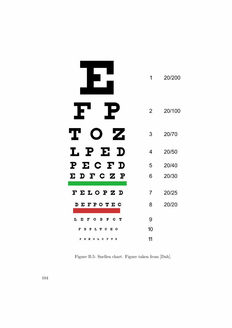
Figure B.5: Snellen chart. Figure taken from [Dah].
104
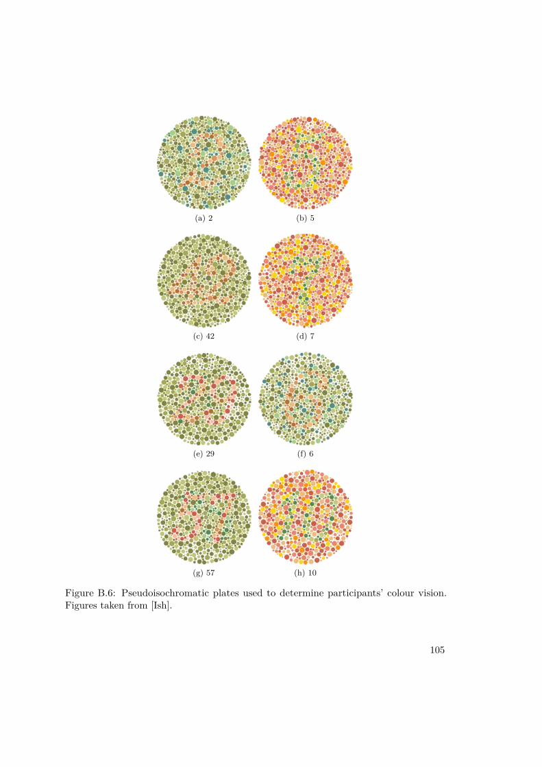
(a) 2 (b) 5
(c) 42 (d) 7
(e) 29 (f) 6
(g) 57 (h) 10
Figure B.6: Pseudoisochromatic plates used to determine participants’ colour vision.Figures taken from [Ish].
105
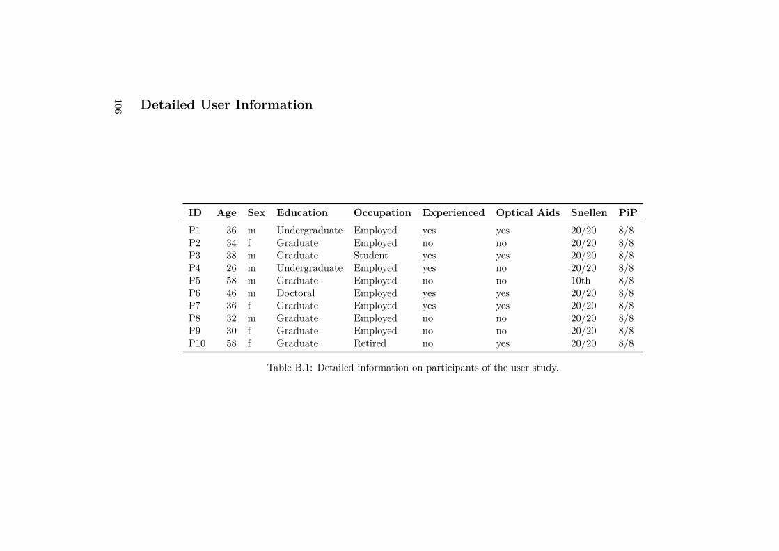
Detailed User Information
ID Age Sex Education Occupation Experienced Optical Aids Snellen PiP
P1 36 m Undergraduate Employed yes yes 20/20 8/8P2 34 f Graduate Employed no no 20/20 8/8P3 38 m Graduate Student yes yes 20/20 8/8P4 26 m Undergraduate Employed yes no 20/20 8/8P5 58 m Graduate Employed no no 10th 8/8P6 46 m Doctoral Employed yes yes 20/20 8/8P7 36 f Graduate Employed yes yes 20/20 8/8P8 32 m Graduate Employed no no 20/20 8/8P9 30 f Graduate Employed no no 20/20 8/8P10 58 f Graduate Retired no yes 20/20 8/8
Table B.1: Detailed information on participants of the user study.
106