Evaluation and Flight Assessment of a Scale Glider

Dissertations and Theses

8-2014

Evaluation and Flight Assessment of a Scale Glider Evaluation and Flight Assessment of a Scale Glider

Alvydas Anthony Civinskas Embry-Riddle Aeronautical University - Daytona Beach

Follow this and additional works at: https://commons.erau.edu/edt

Part of the Aerospace Engineering Commons

Scholarly Commons Citation Scholarly Commons Citation Civinskas, Alvydas Anthony, "Evaluation and Flight Assessment of a Scale Glider" (2014). Dissertations and Theses. 41. https://commons.erau.edu/edt/41

This Thesis - Open Access is brought to you for free and open access by Scholarly Commons. It has been accepted for inclusion in Dissertations and Theses by an authorized administrator of Scholarly Commons. For more information, please contact [email protected].

http://commons.erau.edu/

http://commons.erau.edu/

https://commons.erau.edu/edt

https://commons.erau.edu/edt?utm_source=commons.erau.edu%2Fedt%2F41&utm_medium=PDF&utm_campaign=PDFCoverPages

http://network.bepress.com/hgg/discipline/218?utm_source=commons.erau.edu%2Fedt%2F41&utm_medium=PDF&utm_campaign=PDFCoverPages

https://commons.erau.edu/edt/41?utm_source=commons.erau.edu%2Fedt%2F41&utm_medium=PDF&utm_campaign=PDFCoverPages

mailto:[email protected]

Evaluation and Flight Assessment of a Scale Glider

by

Alvydas Anthony Civinskas

A Thesis Submitted to the College of Engineering Department of Aerospace Engineering

in Partial Fulfillment of the Requirements for the Degree of

Master of Science in Aerospace Engineering

Embry-Riddle Aeronautical University

Daytona Beach, Florida

August 2014

iii

Acknowledgements

The first person I would like to thank is my committee chair Dr. William

Engblom for all the help, guidance, energy, and time he put into helping me. I would also

like to thank Dr. Hever Moncayo for giving up his time, patience, and knowledge about

flight dynamics and testing. Without them, this project would not have materialized nor

survived the many bumps in the road.

Secondly, I would like to thank the RC pilot Daniel Harrison for his time and

effort in taking up the risky and stressful work of piloting. Individuals like Jordan

Beckwith and Travis Billette cannot be forgotten for their numerous contributions in

getting the motor test stand made and helping in creating the air data boom pod so that

test data.

Thirdly, I cannot forget the help from Jade McClanahan, Israel Mogul, Andres

Perez, and Dr. Glenn Greiner for their input and insight.

Lastly, I cannot forget the people who supported me throughout this project: my

family, Michael Carkin, Aliraza Rattansi, Tsewang Shrestha, Killian Marie, and

Mohannad Mahdi.

iv

“In theory, there is no difference between theory and practice. But in

practice, there is.”

― Yogi Berra

https://www.goodreads.com/author/show/79014.Yogi_Berra

v

Abstract

Researcher: Alvydas Anthony Civinskas

Title: Evaluation and Flight Assessment of a Scale Glider.

Institution: Embry-Riddle Aeronautical University

Degree: Master of Science in Aerospace Engineering

Year: 2014

The objective of this project is to do a flight assessment of a Phoenix K8B radio

controlled glider to see what process is needed to verify its glide slope and stability

characteristics. The flight test analysis, plus a computational fluid dynamics analysis, and

an industry-like component build-up aerodynamic analysis were done to provide

comparable estimates for the aircraft glide slope. A stability and control derivative

analysis was also completed and compared using SURFACES, USAF Datcom, and MIT

AVL software. The glide slope estimate and stability and control derivatives obtained

from flight test data showed considerable range and uncertainty. Potential sources of

noisy test data and model flaws are discussed in detail. Improvements to the flight test

capability are suggested.

vi

Table of Contents

Page

Thesis Review Committee .................................................................................................. ii

Acknowledgements ............................................................................................................ iii

Abstract .............................................................................................................................. iv

List of Tables ..................................................................................................................... ix

List of Figures ......................................................................................................................x

Nomenclature .....................................................................................................................xv

List of Acronyms and Abbreviations .............................................................................. xvii

Chapter

1 Introduction ..................................................................................................1

2 Methodology ................................................................................................2

2.1 Airframe Analysis ............................................................................2

2.2 Center of Gravity Calculation ..........................................................4

2.3 Electronics Arrangement .................................................................7

2.4 Instrumentation ..............................................................................11

2.4.1 APM 2.5 .............................................................................11

2.4.2 Air Data Boom ...................................................................14

2.4.3 Pitot Tube ...........................................................................16

2.4.4 Angle of Attack and Angle of Yaw Vane ..........................17

2.4.5 Air Data Boom Pod ............................................................19

2.4.6 GPS ....................................................................................26

2.5 Computational Fluid Dynamics (CFD) Model ..............................26

vii

2.6 3D Computational Fluid Dynamic (CFD) Analysis ......................30

2.7 Component Build-up (Industry) Approach ....................................31

2.8 Aero and Stability Characteristics from Computer Models ...........34

2.8.1 SURFACES .......................................................................34

2.8.2 AVL ...................................................................................37

2.8.3 USAF Digital Datcom........................................................39

2.8.4 MATLAB/Simulink Model ...............................................42

2.9 Motor Testing.................................................................................48

2.10 Flight Test ......................................................................................50

2.10.1 Takeoff ...............................................................................50

2.10.2 Maneuvers ..........................................................................53

2.10.3 Data ....................................................................................55

3. Results ........................................................................................................56

3.1 Stability Results Comparison .........................................................56

3.2 Glide Slope Comparison ................................................................56

4. Conclusions ................................................................................................73

5. Future Work ...............................................................................................74

References ..........................................................................................................................76

Appendices

A Flight Test Data..........................................................................................79

a. April 30th

2014 ...............................................................................79

b. May 8th

2014 – 1 ............................................................................86

c. May 8th

2014 – 2 ............................................................................93

viii

B Datcom Graphs ........................................................................................101

C Pilot Inputs ...............................................................................................106

a. Flight test on April 30th

2014 .......................................................106

b. Flight test on May 8th

2014 - 1 .....................................................107

c. Flight test on May 8th

2014 – 2 ....................................................109

D Graphs for Simulink Model .....................................................................111

a. Stability Derivatives.....................................................................111

b. Trimmed Model Graphs ...............................................................112

c. Doublet Graphs ............................................................................113

E Optimization ............................................................................................115

F Stability Derivatives Comparison ............................................................116

G Scripts ......................................................................................................118

ix

List of Tables

Page

Table

1 Basic Dimensions of K8b RC Glider [6] ...................................................................................... 3

2 Electronic item list ................................................................................................................................ 8

3 Electronic item list for autopilot and tethered configuration ............................................. 10

4 Experimental data for airspeed calibration ............................................................................... 16

5 Experimental data for AoA calibration ...................................................................................... 19

6 Experimental data for AoY calibration ...................................................................................... 19

7 Specifications of the MediaTek MT3329 GPS without any type of augmentation

[41] ........................................................................................................................................................... 26 8 Wing measurements [3].................................................................................................................... 29

9 Aircraft geometry [9]......................................................................................................................... 32

10 Flight Conditions [9] ......................................................................................................................... 32

11 Tail and fuselage contribution values [9] .................................................................................. 32

12 Reference geometry value used in SURFACES ..................................................................... 36

13 Reference information used in SURFACES ............................................................................ 37

14 Inertias calculated by SURFACES .............................................................................................. 37

15 Damping ratios for both modes using the stability derivatives in Appendix D .......... 48

16 Experimental data for motor testing ............................................................................................ 49

17 Items in bungee launch system ...................................................................................................... 52

18 Glide slope comparison .................................................................................................................... 73

x

List of Figures

Page

Figure

1 From left to Right - Lockheed Martin Hale-D, Titan Aerospace Solara, and Ascenta

[14 ,12 , 13] .............................................................................................................................................. 1 2 Previous aircraft design work [4]. ................................................................................................... 2

3 HQ 3.0/15.0 airfoil profile [9]........................................................................................................... 3

4 Fully assembled glider ......................................................................................................................... 3

5 Computerscales AccuSet [19] ........................................................................................................... 4

6 Glider on the scales ............................................................................................................................... 4

7 FBD to figure out the CG ................................................................................................................... 5

8 Electronic schematic ............................................................................................................................. 7

9 Upgradable electronic schematic ..................................................................................................... 9

10 Overview of the Simulink wiring diagram for data recording .......................................... 11

11 Blocks for clock, real time monitor, and the IMU with a complementary filter ........ 12

12 Part of the wiring diagram showing GPS and barometer .................................................... 12

13 Part of schematic showing the three analog inputs - AoA, AoY, airspeed - and pilot

inputs ....................................................................................................................................................... 13 14 Blocks that print the data to IDE via serial and record data to flash memory ............. 13

15 Air Data vane assembly with AoA vane, AoY vane, and Pitot system ......................... 14

16 AoA error contour taken from a slice of the 3D wing near the wing tip [9, 37] ........ 15

17 Calibration setup for air data boom ............................................................................................. 16

18 Graphical representation of the experimental data with the linear regression equation

.................................................................................................................................................................... 17

xi

19 Graphical representation of the experimental data with the linear regression equation

.................................................................................................................................................................... 18 20 Graphical representation of experimental data with regression line ............................... 18

21 Side view of air data boom pod with wingtip outline ........................................................... 19

22 Top view with a 12 inch ruler for reference ............................................................................. 20

23 Hot wire tool ......................................................................................................................................... 20

24 Vacuum bagging air data pod ........................................................................................................ 21

25 Air data pod vacuum bagged in oven .......................................................................................... 21

26 Mapping of the inside the air data boom pod ........................................................................... 22

27 Both halves of the air data pod ...................................................................................................... 22

28 Side view of air data pod ................................................................................................................. 23

29 Aligning air data boom pod ............................................................................................................ 23

30 Leveling the glider ............................................................................................................................. 24

31 Leveling wing for aligning the air data pod .............................................................................. 24

32 Aligning the air data boom pod ..................................................................................................... 25

33 The assembled air data boom on the wingtip of the glider ................................................. 25

34 The laser 3D scanner Faro arm [3] ............................................................................................... 27

35 3D laser scan of the vertical tail section [3] ............................................................................. 28

36 Post processing of completed model for the vertical tail [3] .............................................. 28

37 CATIA model views of the wing [3] .......................................................................................... 29

38 Completed model for CFD [3] ....................................................................................................... 30

39 3D CFD grid [9] .................................................................................................................................. 31

40 Coefficient of lift versus angle of attack .................................................................................... 33

41 Drag coefficient for the whole aircraft versus angle of attack ........................................... 33

xii

42 Lift to drag ratio versus angle of attack ...................................................................................... 34

43 Isometric view of SURFACES model ........................................................................................ 35

44 Side view of SURFACES model .................................................................................................. 35

45 Top view of SURFACES model ................................................................................................... 36

46 Isometric view of AVL model ....................................................................................................... 38

47 Top View of AVL model ................................................................................................................. 38

48 Side View of AVL model ................................................................................................................ 39

49 Isometric view generated by MATLAB .................................................................................... 40

50 Side View generated by MATLAB ............................................................................................. 40

51 Front View generated by MATLAB ........................................................................................... 41

52 Top View generated by MATLAB .............................................................................................. 41

53 Simulink model for figuring out the aircraft response.......................................................... 42

54 Blocks that need to be changed ..................................................................................................... 43

55 Inside Autopilot Block to change all the gains to the appropriate values ..................... 43

56 Inside the Cable & Actuator Dynamics block to change the force gain so that the

altitude is trimmed for level flight ................................................................................................ 44 57 Step function input in radians ........................................................................................................ 44

58 An example of how alpha should respond to a step function [20] ................................... 45

59 Alpha response of the Simulink model to the step function input at one second ....... 46

60 A longer time period response to the step function input for alpha ................................. 46

61 Airspeed response from step function input ............................................................................. 47

62 Electronic Schematic for propeller testing ................................................................................ 48

63 Experimental setup in the wind tunnel ....................................................................................... 49

64 Graphical representation of experimental data ........................................................................ 50

xiii

65 Bungee system diagram for takeoff ............................................................................................. 53

66 Pitch doublet ......................................................................................................................................... 54

67 Yaw doublet .......................................................................................................................................... 54

68 Roll doublet ........................................................................................................................................... 55

69 Selected altitude .................................................................................................................................. 57

70 Selected altitude close up ................................................................................................................. 58

71 Air speed and ground speed ............................................................................................................ 58

72 Wind speed from the difference of airspeed and ground speed ........................................ 59

73 Pilot inputs ............................................................................................................................................. 60

74 Measured angle of attack ................................................................................................................. 60

75 Selected altitude .................................................................................................................................. 61

76 Close up of selected altitude range............................................................................................... 61

77 Pilot Inputs ............................................................................................................................................ 62

78 Measured angle of attack ................................................................................................................. 62

79 Air speed and ground speed comparison ................................................................................... 63

80 Comparison of selected ranges ...................................................................................................... 63

81 Comparison of pilot inputs for selected ranges ....................................................................... 64

82 Comparison of angle of attack among selected ranges ........................................................ 64

83 Linear regression line for selected range ................................................................................... 66

84 Instantaneous L/D with error bars ................................................................................................ 67

85 Error in L/D........................................................................................................................................... 68

86 Wind direction by taking the difference of air and ground speed .................................... 68

87 Residuals to tell how well the linear regression line fits the model ................................ 69

xiv

88 Same selected altitude range but with a 2nd order polynomial fit regression line .... 70

89 Instantaneous L/D with error bars ................................................................................................ 70

90 Error in L/D........................................................................................................................................... 71

91 Residual plot for the 2nd order polynomial fit regression .................................................. 71

xv

Nomenclature

Dcg: distance of center of gravity

WT: total weight of aircraft

Wn: weight of nose section

Wt: weight of tail section

dn: distance of nose weight measurement

dt: distance of tail weight measurement

ID: inner diameter

OD: outer diameter

L: length

x,y,z: measurement quantities

x, y, z: errors associated with quantities measured

: damping ratio

T: thrust

T0: static thrusat

W: weight

S: planform area

: air density at sea level

CLg: ground coefficient of lift

CDg: ground drag coefficient

a: constant with units of lb*s2/ft2

: runway friction coefficient

V: velocity

xvi

VT0: take off velocity

g: acceleration due to gravity

xvii

List of Acronyms and Abbreviations

CFD: Computational Fluid Dynamics

DAP: Dual Aircraft Platform

UAV: Unmanned Ariel Vehicle

RC: Radio Controlled

ARFT: Almost Ready to Fly

HQ: Helmut Quabeck

CG: Center of Gravity

FBD: Free Body Diagram

APM: Ardupilot Mega

IMU: Inertial Measurement Unit

GPS: Global Positioning System

SSH: Secure Shell

IDE: Integrated Development Environment

AoA: Angle of Attack

AoY: Angle of Yaw

EFRC: Eagle Flight Research Center

NURB: Non-uniform Rational B-spline

CATIA: Computer Aided Three-dimensional Interactive Application

NACA: National Advisory Commit for Aeronautics

USAF: United States Air Force

VLM: Vortex Lattice Method

ID: Inner Diameter

xviii

OD: Outer Diameter

LE: Leading Edge

ICAO: International Civil Aviation Organization

NP: Neutral Point

RMS: Root Mean Square

1

1. Introduction

The objective of this project is to compare the results of the glide slope among

flight-testing, computational fluid dynamics (CFD), and a conventional aerodynamic

build-up approach for a scale model powered glider. This assessment is relevant because

determining the accuracy will influence a designer’s reliance on a particular method in

predicting the glide slope of an aircraft. The motivation for this project is the Dual

Aircraft Platform (DAP) configuration that relies heavily on a high lift-to-drag ratio to

permit sailing type operation within the stratosphere using the least possible use of

energy to stay aloft [28]. The lower the glide slope for the design translates into a higher

available wind shear needed for the DAP to be an effective atmospheric satellite therefore

potentially limiting the area where the DAP could be used [4]. In essence, knowing an

accurate glide slope is crucial for the operating capability for the DAP [4].

Recently, both Google and Facebook acquired drone companies so that both

companies could utilize these atmospheric satellites to increase access to the Internet [12,

13]. Google specifically bought Titan Aerospace for that purpose [12]. The Titan Solara

can cover as much ground as 100 based towers and carry a capacity of 70lb with the

Solara 50 and 250lbs with the Solara 60 model [12]. Figure 1 shows Lockheed’s, Titan’s,

and Ascenta’s concepts for atmospheric satellites, respectively.

Figure 1: From left to Right - Lockheed Martin Hale-D, Titan Aerospace Solara, and Ascenta [14 ,12

, 13]

2

2. Methodology

2.1. Airframe Analysis

A previous graduate student at Embry Riddle provided a design of the aircraft. It

utilized a tandem wing configuration to maximize lift by using the Wortmann FX 63-137

airfoil and is shown in Figure 2 [4]:

Figure 2: Previous aircraft design work [4].

Due to the limited funding available to build the unmanned aerial vehicle (UAV)

from scratch utilizing carbon fiber, it was decided to find a pre-existing design on the

market that satisfied the 2 m2 wing planform area needed to satisfy the goals of the DAP

program for a sub-scale aircraft. The Phoenix model K8B 6m almost ready to fly (ARFT)

was chosen primarily for its wing area of 2.26 m2 (3503 in

2) and airframe price. This

model is a 40% scaled version of the Alexander Schleicher Ka 8b glider [3, 6]. This radio

controller (RC) glider uses the HQ 3/15 airfoil, which the outline of the airfoil is depicted

in Figure 3:

3

Figure 3: HQ 3.0/15.0 airfoil profile [9]

This airfoil also goes under the names of HQ 3.0/15.0 and HQ 3015. Table 1 shows the

specifications of the model selected from the Phoenix Model website:

Phoenix K8b - 6m Specifications

Wing Span 6m

Wing Area 219.4 dm2

Length 2873mm

Wing Loading 64 g/dm2

Flying Weight 14-18 kg

Scale 1/2.5

Wing Airfoil HQW 3/15 [35] Table 1: Basic Dimensions of K8b RC Glider [6]

Figure 4 shows the assembled glider.

Figure 4: Fully assembled glider

4

2.2 Center of Gravity Calculation

A critical piece of information for an aircraft is the location of the center of

gravity (CG). To find the CG, the Computerscales AccuSet instrument pictured in Figure

5 was used:

Figure 5: Computerscales AccuSet [19]

One scale was placed below the tail section while another was placed under the cockpit.

Any piece of equipment that was going to be utilized in the UAV was put into its place as

and assembled as shown in Figure 6:

Figure 6: Glider on the scales

5

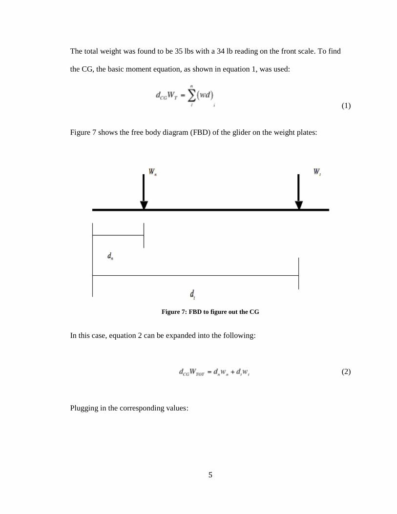
The total weight was found to be 35 lbs with a 34 lb reading on the front scale. To find

the CG, the basic moment equation, as shown in equation 1, was used:

(1)

Figure 7 shows the free body diagram (FBD) of the glider on the weight plates:

Figure 7: FBD to figure out the CG

In this case, equation 2 can be expanded into the following:

(2)

Plugging in the corresponding values:

6

(3)

(4)

(5)

The recommended CG location is 150mm from the LE with a margin of +/- 5mm.

[22]. Subtracting 26 inches from 31.89 gives a distance of 5.89 inches from the LE. The

mean aerodynamic chord (MAC) was found to be 14.99 in. An estimation of where the

neutral point (NP) must be calculated to find the static margin. An online calculator

utilizing a panel method was used to find the AC at 3.75 inches aft of the LE while the

NP was 7.82 inches [25]. Finding the difference between the CG and NP and dividing

that result by the MAC found a static margin of 12.88% of the MAC. Since the

configuration changed with a pound of weight added to the wing of the aircraft, only a

quick calculation was made to see how much the CG moved. In this case, the static

margin increased to 13.25%.

7

2.3 Electronics Arrangement

The overall schematic of all the electronics in the UAV is shown in Figure 8.

Figure 8: Electronic schematic

8

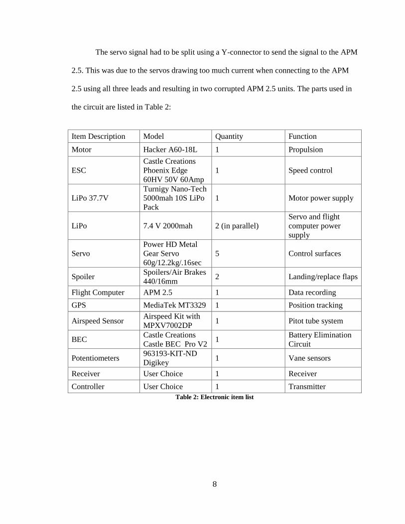
The servo signal had to be split using a Y-connector to send the signal to the APM

2.5. This was due to the servos drawing too much current when connecting to the APM

2.5 using all three leads and resulting in two corrupted APM 2.5 units. The parts used in

the circuit are listed in Table 2:

Item Description Model Quantity Function

Motor Hacker A60-18L 1 Propulsion

ESC

Castle Creations

Phoenix Edge

60HV 50V 60Amp

1 Speed control

LiPo 37.7V

Turnigy Nano-Tech

5000mah 10S LiPo

Pack

1 Motor power supply

LiPo 7.4 V 2000mah 2 (in parallel)

Servo and flight

computer power

supply

Servo

Power HD Metal

Gear Servo

60g/12.2kg/.16sec

5 Control surfaces

Spoiler Spoilers/Air Brakes

440/16mm 2 Landing/replace flaps

Flight Computer APM 2.5 1 Data recording

GPS MediaTek MT3329 1 Position tracking

Airspeed Sensor Airspeed Kit with

MPXV7002DP 1 Pitot tube system

BEC Castle Creations

Castle BEC Pro V2 1

Battery Elimination

Circuit

Potentiometers 963193-KIT-ND

Digikey 1 Vane sensors

Receiver User Choice 1 Receiver

Controller User Choice 1 Transmitter

Table 2: Electronic item list

9

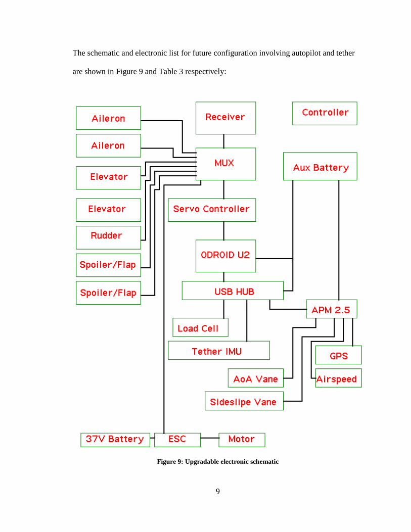
The schematic and electronic list for future configuration involving autopilot and tether

are shown in Figure 9 and Table 3 respectively:

Figure 9: Upgradable electronic schematic

10

Item Description Model Quantity Function

Motor Hacker A60-18L 1 Propulsion

ESC

Castle Creations

Phoenix Edge

60HV 50V 60Amp

1 Speed control

LiPo 37.7V

Turnigy Nano-Tech

5000mah 10S LiPo

Pack

1 Motor power supply

Aux Battery 2

Servo, sensor, and

flight computer

power supply

Servo

Power HD Metal

Gear Servo

60g/12.2kg/.16sec

5 Control surfaces

USB Hub 10 Port USB 2.0

Hub by FDL 1 USB Hub

16 Channel Servo

Controller Cytron SC16A 1 Servo Controller

ODROID U2

ODRIOD U2 -

ULTRA

COMPACT

1.7GHz QUAD-

CORE BOARD

1 Flight computer

9 DoF IMU 9DOF Razor IMU 1 Tether IMU

Multiplexer (MUX) Cytron 8 Channel

RC RX Multiplexer 1

Switch between

autopilot and manual

control

Spoiler Spoilers/Air Brakes

440/16mm 2 Landing/replace flaps

Flight Computer APM 2.5 1 Data recording and

autopilot

GPS w/ compass uBlox LEA-6H

module 1 Position tracking

Potentiometers 963193-KIT-ND

Digikey 1 Vane sensors

BEC Castle Creations

Castle BEC Pro V2 1

Battery Elimination

Circuit

Receiver User choice 1 Receiver

Controller User choice 1 Controller

Table 3: Electronic item list for autopilot and tethered configuration

11

2.4 Instrumentation

2.4.1 APM 2.5

The data collecting unit used for this project was the APM 2.5 loaded with a

Mathworks Simulink toolbox created for the APM by previous Embry Riddle students

called APM2 Simulink Blockset.

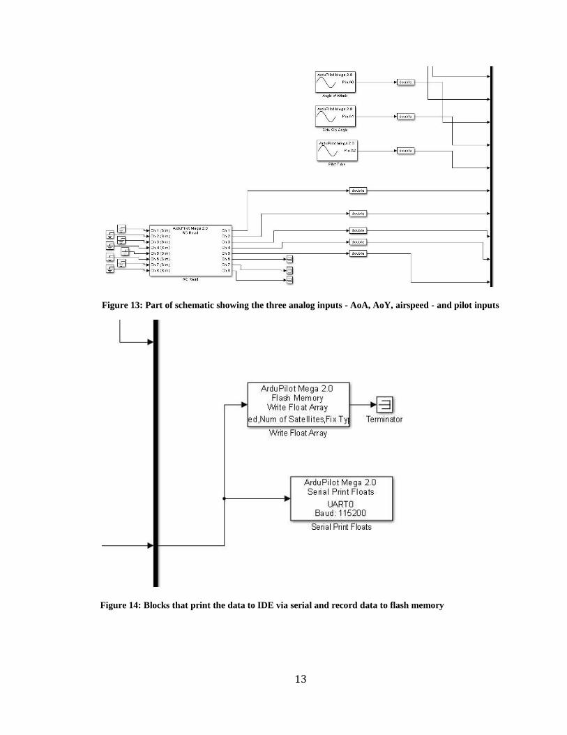
The blocks that were included were the IMU, GPS, barometer, and three analog

inputs, and RC Read. For data recording, a ‘Flash’ block is required for data collection.

The ‘Serial Print Floats’ block was used so that the data can be printed out as text using

either Putty, an SSH secure wrapper, or the Arduino IDE at a serial baud rate of 115200.

Figure 10 shows the Simulink model used for data recording:

Figure 10: Overview of the Simulink wiring diagram for data recording

12

Figure 11: Blocks for clock, real time monitor, and the IMU with a complementary filter

The complementary filter was chosen because none of the sensors’ data were used for

navigation purposes [38]. The filter should have both accelerometer and gyro data

feeding into it to calculate both phi and theta [36].

Figure 12: Part of the wiring diagram showing GPS and barometer

13

Figure 13: Part of schematic showing the three analog inputs - AoA, AoY, airspeed - and pilot inputs

Figure 14: Blocks that print the data to IDE via serial and record data to flash memory

14

2.4.2 Air Data Boom

The air data boom consists of two potentiometers from CTS Electrocomponents,

two 3D printed vanes, two 3D printed pieces for the boom structure, and an airspeed

sensor kit from 3Drobotics that included a Pitot static tube. Figure 15 shows the pieces

that make up the air data boom in the wind tunnel:

Figure 15: Air Data vane assembly with AoA vane, AoY vane, and Pitot system

15

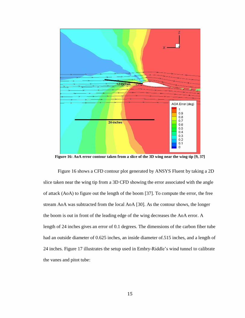
Figure 16: AoA error contour taken from a slice of the 3D wing near the wing tip [9, 37]

Figure 16 shows a CFD contour plot generated by ANSYS Fluent by taking a 2D

slice taken near the wing tip from a 3D CFD showing the error associated with the angle

of attack (AoA) to figure out the length of the boom [37]. To compute the error, the free

stream AoA was subtracted from the local AoA [30]. As the contour shows, the longer

the boom is out in front of the leading edge of the wing decreases the AoA error. A

length of 24 inches gives an error of 0.1 degrees. The dimensions of the carbon fiber tube

had an outside diameter of 0.625 inches, an inside diameter of.515 inches, and a length of

24 inches. Figure 17 illustrates the setup used in Embry-Riddle’s wind tunnel to calibrate

the vanes and pitot tube:

16

Figure 17: Calibration setup for air data boom

2.4.3 Pitot tube

The pitot tube used and tested was from an airspeed sensor kit from 3DRobotics

that utilized the MPXV7002DP chip as its differential pressure sensor. It was placed at

the tip of the air boom to make sure that it was away from the propeller and other

downwash effects from the propeller. The sensor was then connected to the APM 2.5 via

an analog input slot.

Airspeed (mph) Output (V)

0 2.63

10 2.65

20 2.69

30 2.74

40 2.78 Table 4: Experimental data for airspeed calibration

17

Figure 18: Graphical representation of the experimental data with the linear regression equation

2.4.4 Angle of Attack and Side Slip Vane Calibration

The AoA and angle of yaw (AoY) sensors are just potentiometers with vanes that

are glued onto the tabs. The data collected in Table 5, Table 6, Figure 19, and Figure 20

had the wind tunnel speed set at a constant 10 mph. A positive angle for the AoA vane

indicated that the nose was pitching up. For the AoY, a positive angle meant the nose

yawed to the right.

y = 267.33x - 701.25

0

5

10

15

20

25

30

35

40

45

2.6 2.65 2.7 2.75 2.8

Air

spe

ed

(m

ph

)

Output Voltage (V)

Airspeed vs Output Voltage

Airspeed

Linear (Airspeed)

18

Figure 19: Graphical representation of the experimental data with the linear regression equation

Figure 20: Graphical representation of experimental data with regression line

AoA (alpha) Output (V)

0 4.38

5 4.42

10 4.49

15 4.59

18.8 4.67

y = 62.583x - 272.44

0

5

10

15

20

25

4.3 4.4 4.5 4.6 4.7

Ao

A (

de

g)

Output Voltage (V)

AoA vs Output Voltage

AoA

Linear (AoA)

y = -16.903x + 58.094

-15

-10

-5

0

5

10

15

2.75 3.25 3.75 4.25

Ao

Y (

de

g)

Output Voltage (V)

AoY vs Ouput Voltage

AoY

Linear (AoY)

19

Table 5: Experimental data for AoA calibration

Side Slip/Beta

(deg) Output (V)

-10 3.98

-5 3.67

0 3.59

5 3.10

10 2.84 Table 6: Experimental data for AoY calibration

However, the airspeed should have been set to 25 mph because the vanes were designed

for that velocity [36].

2.4.5 Air Data Boom Pod

The air data boom pod was made out of Styrofoam and fiberglass chop mat. The

first step in the process was to trace an outline of the tip of the wing. Then the Styrofoam

block was sanded down into the desired shape as shown in Figure 21 and Figure 22:

Figure 21: Side view of air data boom pod with wingtip outline

20

Figure 22: Top view with a 12 inch ruler for reference

The next step was to use a hot wire tool in Figure 23 and cut the Styrofoam pod into two

pieces:

Figure 23: Hot wire tool

The fiberglass pieces were then laid on top of each piece of the mold once layer at a time

and vacuum bagged before they were placed into the oven as Figure 24 and Figure 25

show:

21

Figure 24: Vacuum bagging air data pod

Figure 25: Air data pod vacuum bagged in oven

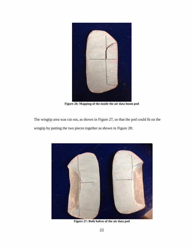
Lines were drawn to map out where wingtip would be placed as shown in Figure 26:

22

Figure 26: Mapping of the inside the air data boom pod

The wingtip area was cut out, as shown in Figure 27, so that the pod could fit on the

wingtip by putting the two pieces together as shown in Figure 28:

Figure 27: Both halves of the air data pod

23

Figure 28: Side view of air data pod

The next step was to make sure that the pod was aligned with the wing at the same pitch

angle of 7 degrees and at the same yaw angle by using a right angle in Figure 29:

Figure 29: Aligning air data boom pod

24

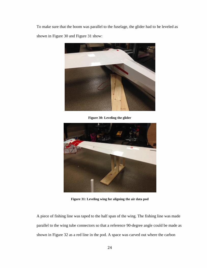
To make sure that the boom was parallel to the fuselage, the glider had to be leveled as

shown in Figure 30 and Figure 31 show:

Figure 30: Leveling the glider

Figure 31: Leveling wing for aligning the air data pod

A piece of fishing line was taped to the half span of the wing. The fishing line was made

parallel to the wing tube connectors so that a reference 90-degree angle could be made as

shown in Figure 32 as a red line in the pod. A space was carved out where the carbon

25

fiber tube and airspeed sensor were placed along with any wires from the AoA and AoY

vanes.

Figure 32: Aligning the air data boom pod

The last step is to put all these pieces together and mount the pod onto the wingtip as

shown in Figure 33:

Figure 33: The assembled air data boom on the wingtip of the glider

26

2.4.6 GPS

The GPS used for data collecting was the MediaTek MT3329. This was used to

capture the location of the UAV and the ground speed. The GPS was checked by cross

checking the lateral and longitudinal coordinates at a known location. The performance

of the GPS chip can be found in from its data sheet as shown in Table 7:

Performance Characteristics

Position Accuracy 3m 2D-RMS

Velocity Accuracy 0.1 m/s

Acceleration Accuracy 0.1 m/s²

Timing Accuracy 100 ns RMS

Table 7: Specifications of the MediaTek MT3329 GPS without any type of augmentation [41]

2.5 Computational Fluid Dynamics (CFD) Model

For the purposes of obtaining estimates for the mass moment of inertias and for

CFD analysis, a surface model of the RC glider was created by using the FARO

PlatniumArm 3D laser scanner at Embry Riddle’s Eagle Flight Research Center (EFRC)

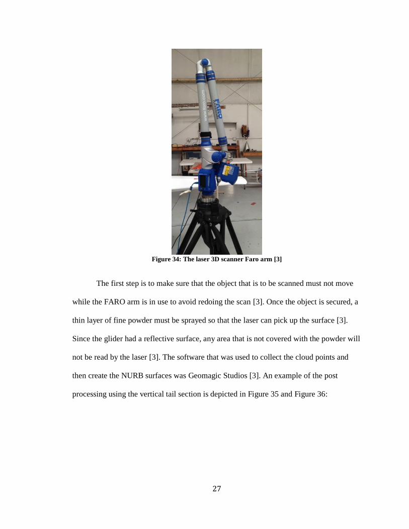
[3]. The arm has an accuracy of +/- 0.029mm [3].

27

Figure 34: The laser 3D scanner Faro arm [3]

The first step is to make sure that the object that is to be scanned must not move

while the FARO arm is in use to avoid redoing the scan [3]. Once the object is secured, a

thin layer of fine powder must be sprayed so that the laser can pick up the surface [3].

Since the glider had a reflective surface, any area that is not covered with the powder will

not be read by the laser [3]. The software that was used to collect the cloud points and

then create the NURB surfaces was Geomagic Studios [3]. An example of the post

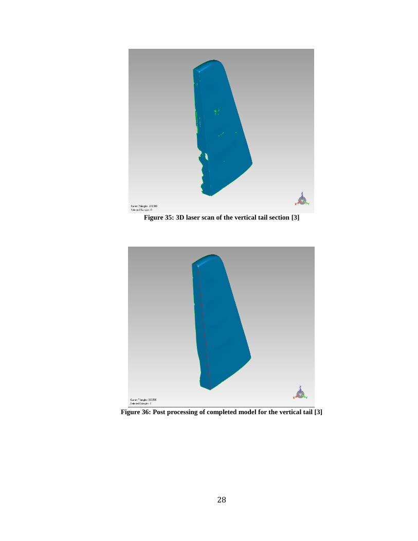
processing using the vertical tail section is depicted in Figure 35 and Figure 36:

28

Figure 35: 3D laser scan of the vertical tail section [3]

Figure 36: Post processing of completed model for the vertical tail [3]

29

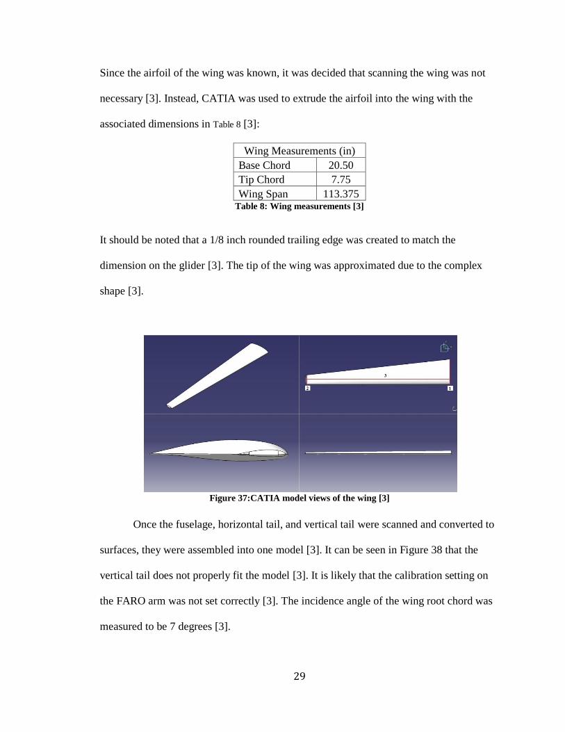
Since the airfoil of the wing was known, it was decided that scanning the wing was not

necessary [3]. Instead, CATIA was used to extrude the airfoil into the wing with the

associated dimensions in Table 8 [3]:

Wing Measurements (in)

Base Chord 20.50

Tip Chord 7.75

Wing Span 113.375 Table 8: Wing measurements [3]

It should be noted that a 1/8 inch rounded trailing edge was created to match the

dimension on the glider [3]. The tip of the wing was approximated due to the complex

shape [3].

Figure 37:CATIA model views of the wing [3]

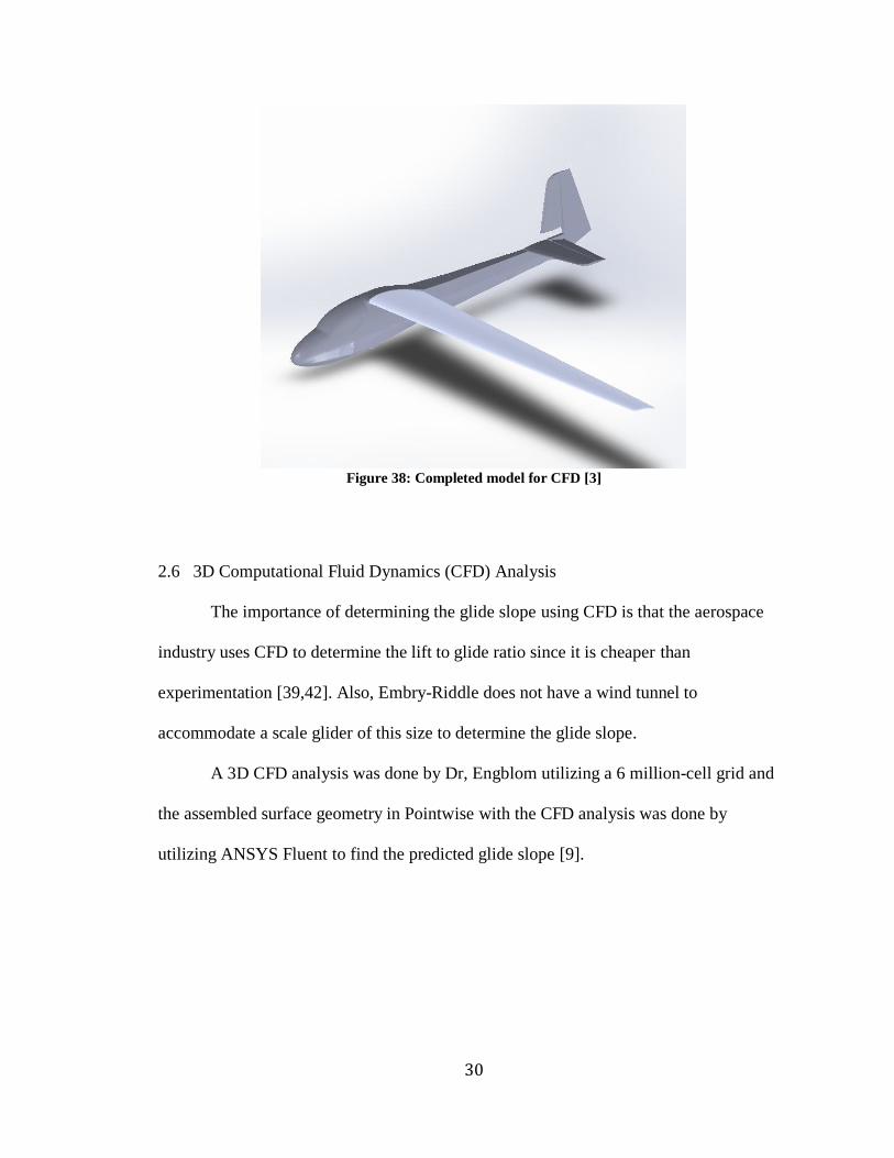
Once the fuselage, horizontal tail, and vertical tail were scanned and converted to

surfaces, they were assembled into one model [3]. It can be seen in Figure 38 that the

vertical tail does not properly fit the model [3]. It is likely that the calibration setting on

the FARO arm was not set correctly [3]. The incidence angle of the wing root chord was

measured to be 7 degrees [3].

30

Figure 38: Completed model for CFD [3]

2.6 3D Computational Fluid Dynamics (CFD) Analysis

The importance of determining the glide slope using CFD is that the aerospace

industry uses CFD to determine the lift to glide ratio since it is cheaper than

experimentation [39,42]. Also, Embry-Riddle does not have a wind tunnel to

accommodate a scale glider of this size to determine the glide slope.

A 3D CFD analysis was done by Dr, Engblom utilizing a 6 million-cell grid and

the assembled surface geometry in Pointwise with the CFD analysis was done by

utilizing ANSYS Fluent to find the predicted glide slope [9].

31

Figure 39: 3D CFD grid [9]

The 3D CFD model predicted a CL of .71 and a CD of .044. This gives an L/D of 16.3 at a

wing alpha of 4 degrees. This is below the glide slope of 25 that was desired [37].

2.7 Component Build-up (Industry) Approach

A conventional approach to calculate the glide slope of an aircraft is to look at an

airfoil’s lift and drag coefficient for each individual component and assume negligible

interactions among the components [9]. The performance for the finite wings in this

assessment are made based on XFOIL airfoil data at Reynolds number of 300,000 and the

affect of induced drag [9].

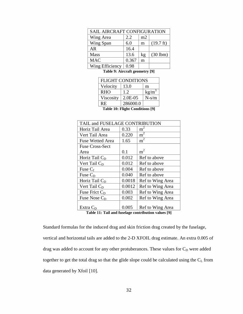
32

SAIL AIRCRAFT CONFIGURATION

Wing Area 2.2 m2

Wing Span 6.0 m (19.7 ft)

AR 16.4

Mass 13.6 kg (30 lbm)

MAC 0.367 m

Wing Efficiency 0.98 Table 9: Aircraft geometry [9]

FLIGHT CONDITIONS

Velocity 13.0 m

RHO 1.2 kg/m3

Viscosity 2.0E-05 N-s/m

RE 286000.0 Table 10: Flight Conditions [9]

TAIL and FUSELAGE CONTRIBUTION

Horiz Tail Area 0.33 m2

Vert Tail Area 0.220 m2

Fuse Wetted Area 1.65 m2

Fuse Cross-Sect

Area 0.1 m2

Horiz Tail CD 0.012 Ref to above

Vert Tail CD 0.012 Ref to above

Fuse Cf 0.004 Ref to above

Fuse CD 0.040 Ref to above

Horiz Tail CD 0.0018 Ref to Wing Area

Vert Tail CD 0.0012 Ref to Wing Area

Fuse Frict CD 0.003 Ref to Wing Area

Fuse Nose CD 0.002 Ref to Wing Area

Extra CD 0.005 Ref to Wing Area Table 11: Tail and fuselage contribution values [9]

Standard formulas for the induced drag and skin friction drag created by the fuselage,

vertical and horizontal tails are added to the 2-D XFOIL drag estimate. An extra 0.005 of

drag was added to account for any other protuberances. These values for CD were added

together to get the total drag so that the glide slope could be calculated using the CL from

data generated by Xfoil [10].

33

Figure 40: Coefficient of lift versus angle of attack

Figure 41: Drag coefficient for the whole aircraft versus angle of attack

-1.0000

-0.5000

0.0000

0.5000

1.0000

1.5000

-15.00 -10.00 -5.00 0.00 5.00 10.00 15.00 20.00

CL

Angle of Attack (deg)

CL vs Angle of Attack

0.0000

0.0200

0.0400

0.0600

0.0800

0.1000

0.1200

-15.00 -10.00 -5.00 0.00 5.00 10.00 15.00 20.00

CD

TO

T


CDTOT vs Angle of Attack

34

Figure 42: Lift to drag ratio versus angle of attack

The maximum glide slope was found to be 23.79. This value is larger than the 16.63

found from using CFD and closer to the desired value of 25. However, both approaches

make assumptions about the geometry and flow conditions like a constant, idealized flow

from one direction and ignoring the imperfections of the scale glider model that make an

accurate estimation from these two methods unreliable.

2.8 Aero and Stability Characteristics from Computer Models

2.8.1 SURFACES

The first and main,Vortex Lattice Method (VLM) program that was used was

SURFACES. Figure 43 through Figure 45 show the model that was created and used in

SURFACES to estimate the inertias and stability derivatives.

-15.00

-10.00

-5.00

0.00

5.00

10.00

15.00

20.00

25.00

30.00

-15.00 -10.00 -5.00 0.00 5.00 10.00 15.00 20.00

L/D


L/D vs Angle of Attack

35

Figure 43: Isometric view of SURFACES model

Figure 44: Side view of SURFACES model

36

Figure 45: Top view of SURFACES model

Table 12 through Table 14 show the reference values used in SURFACES:

Reference Geometry

Reference Chord (MAC), Cref 1.28 ft

Cref start location, Xref 0.00 ft

Reference Span, Bref 19.4 ft

Reference Area, Sref 23.6 ft2

Wetted Area, Swet 47.85 ft2

Table 12: Reference geometry value used in SURFACES

37

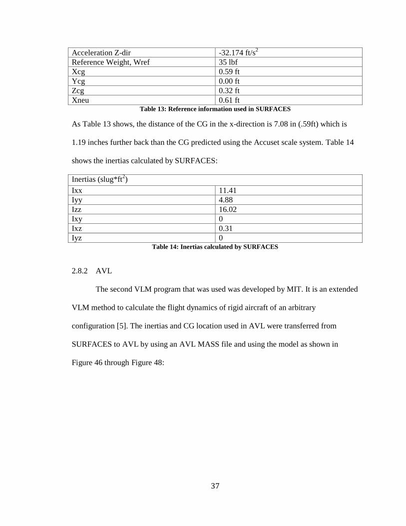
Acceleration Z-dir -32.174 ft/s2

Reference Weight, Wref 35 lbf

Xcg 0.59 ft

Ycg 0.00 ft

Zcg 0.32 ft

Xneu 0.61 ft Table 13: Reference information used in SURFACES

As Table 13 shows, the distance of the CG in the x-direction is 7.08 in (.59ft) which is

1.19 inches further back than the CG predicted using the Accuset scale system. Table 14

shows the inertias calculated by SURFACES:

Inertias (slug*ft2)

Ixx 11.41

Iyy 4.88

Izz 16.02

Ixy 0

Ixz 0.31

Iyz 0 Table 14: Inertias calculated by SURFACES

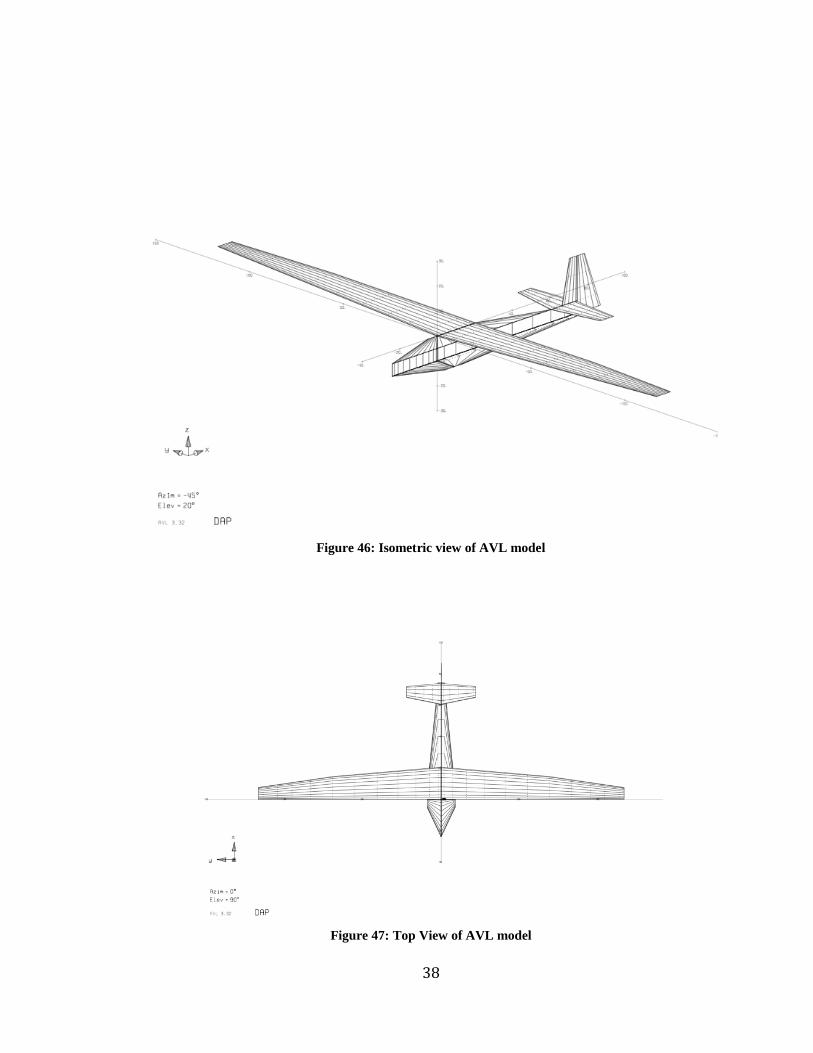
2.8.2 AVL

The second VLM program that was used was developed by MIT. It is an extended

VLM method to calculate the flight dynamics of rigid aircraft of an arbitrary

configuration [5]. The inertias and CG location used in AVL were transferred from

SURFACES to AVL by using an AVL MASS file and using the model as shown in

Figure 46 through Figure 48:

38

Figure 46: Isometric view of AVL model

Figure 47: Top View of AVL model

39

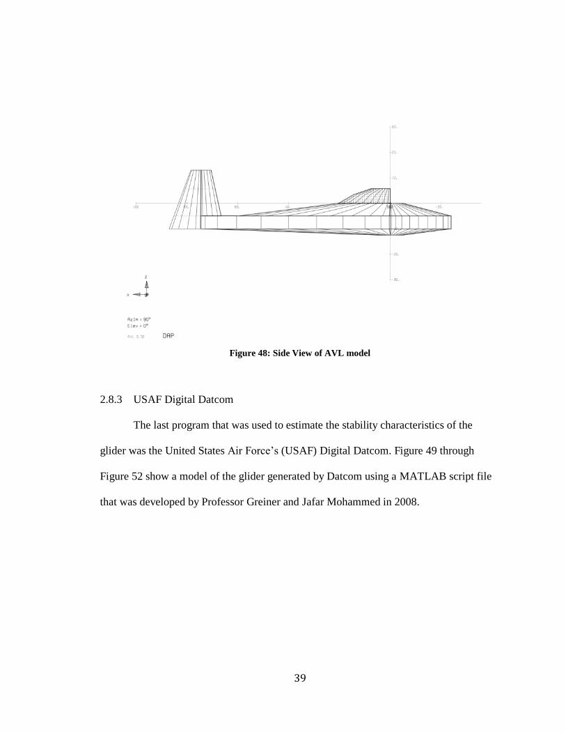
Figure 48: Side View of AVL model

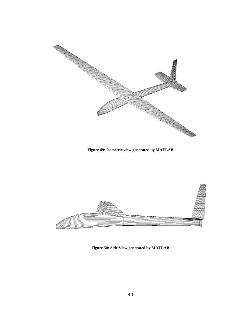
2.8.3 USAF Digital Datcom

The last program that was used to estimate the stability characteristics of the

glider was the United States Air Force’s (USAF) Digital Datcom. Figure 49 through

Figure 52 show a model of the glider generated by Datcom using a MATLAB script file

that was developed by Professor Greiner and Jafar Mohammed in 2008.

40

Figure 49: Isometric view generated by MATLAB

Figure 50: Side View generated by MATLAB

41

Figure 51: Front View generated by MATLAB

Figure 52: Top View generated by MATLAB

It should be noted the HQ 3.0/15.0 airfoil was not used but rather the NACA 6

series airfoil 63(2)-615, which is similar to the HQ airfoil [9]. Evaluation of rudder input

was not available in the software. The graphs generated by Datcom can be found in

Appendix B from the same MATLAB script made possible by Dr. Greiner and Jafar

Mohammad.

The table in Appendix F compares the stability derivatives generated by all three

software packages. Any stability derivative that was on the scale of 10^-5 was deemed to

small and therefore, zero.

42

2.8.4 MATLAB/Simulink Model

An optimization program was planned, but due to noisy flight data and issues with

optimization convergence, as shown in Appendix E, a decision was made to analyze the

dynamic modes of the aircraft - the phugoid, short period, and Dutch-roll. Unfortunately,

only the short and phugoid modes were evaluated but the Dutch-roll mode was found to

be highly unstable based on the derivatives obtained and shown in Appendix D.

The model used to figure out the modes of the aircraft is shown in Figure 53:

Figure 53: Simulink model for figuring out the aircraft response

The first task is to input zero signals into each direction to see if the model is

stable – to see damped oscillations in the longitudinal direction, but zero dynamic

behavior in the lateral direction. These time history figures are provided in Appendix D

along with a table of stability derivatives that were found to make the model stable. The

two blocks whose contents that were modified to make the model stable are shown in

Figure 54:

43

Figure 54: Blocks that need to be changed

Inside the Autopilot block, shown in red in Figure 54, the user must change the gains to

one and negative one as shown in Figure 55:

Figure 55:Inside Autopilot Block to change all the gains to the appropriate values

Inside the blue ‘Cable & Actuator Dynamics’ block, the ‘Force’ gain had to be changed

so that the altitude oscillation leveled off, as shown in Appendix D. In this case, the

‘Force’ gain was set to 20.385 N because the altitude was at level flight as shown in

Appendix D for the trimmed condition.

44

Figure 56: Inside the Cable & Actuator Dynamics block to change the force gain so that the altitude

is trimmed for level flight

After these changes, a step function was introduced into the pitch direction.

Figure 57 shows the step function in radians that was used to excite the response in the

model:

Figure 57: Step function input in radians

0 50 100 150 200 250 300 350

0

1

2

3

4

5

6

7

8

9

x 10-4 Input Function

Time (s)

45

Figure 58 shows an example of how both alpha and q responded to a step response input

function from Eric Watkiss from the Naval Postgraduate School [21]:

Figure 58: An example of how alpha should respond to a step function [20]

Figure 59 and Figure 60 show the response of alpha while the airspeed response is shown

in Figure 61 for the MATLAB model using the stability derivatives in Appendix D:

46

Figure 59: Alpha response of the Simulink model to the step function input at one second

Figure 60: A longer time period response to the step function input for alpha

0 2 4 6 8 10

0.02

0.04

0.06

0.08

0.1

0.12

0.14

0.16

Alpha

Alp

ha (

rad)

Time (s)

0 5 10 15 20 25 30 35 40 45

0

0.05

0.1

0.15

0.2

0.25

0.3

0.35

0.4

Alpha

Alp

ha (

rad)

Time (s)

47

.

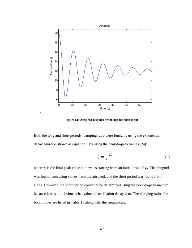
Figure 61: Airspeed response from step function input

Both the long and short periods’ damping ratio were found by using the exponential

decay equation shown as equation 6 by using the peak-to-peak values [24]:

(6)

where y is the final peak value at n cycles starting from an initial peak of y0. The phugoid

was found from using values from the airspeed, and the short period was found from

alpha. However, the short period could not be determined using the peak-to-peak method

because it was not obvious what value the oscillation decayed to. The damping ratios for

both modes are listed in Table 15 along with the frequencies:

0 10 20 30 40 50 60

6

8

10

12

14

16

18

20

Airspeed

Airspeed (

m/s

)

Time (s)

48

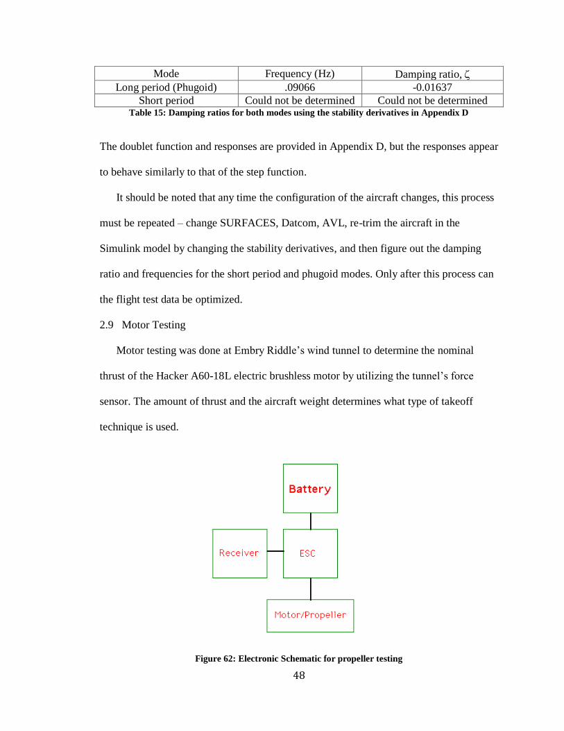
Mode Frequency (Hz) Damping ratio,

Long period (Phugoid) .09066 -0.01637

Short period Could not be determined Could not be determined Table 15: Damping ratios for both modes using the stability derivatives in Appendix D

The doublet function and responses are provided in Appendix D, but the responses appear

to behave similarly to that of the step function.

It should be noted that any time the configuration of the aircraft changes, this process

must be repeated – change SURFACES, Datcom, AVL, re-trim the aircraft in the

Simulink model by changing the stability derivatives, and then figure out the damping

ratio and frequencies for the short period and phugoid modes. Only after this process can

the flight test data be optimized.

2.9 Motor Testing

Motor testing was done at Embry Riddle’s wind tunnel to determine the nominal

thrust of the Hacker A60-18L electric brushless motor by utilizing the tunnel’s force

sensor. The amount of thrust and the aircraft weight determines what type of takeoff

technique is used.

Figure 62: Electronic Schematic for propeller testing

49

Figure 63: Experimental setup in the wind tunnel

As Table 16 and Figure 64 show, the three bladed configuration increases the thrust by

3.81 lbf compared to the two bladed configuration at full throttle and assuming a linear

throttle curve:

2 blades 3 blades

0 10.52 lbf 14.33 lbf

15 9.83 lbf 13.47 lbf

30 7.82 lbf 11.43 lbf Table 16: Experimental data for motor testing

50

Figure 64: Graphical representation of experimental data

2.10 Flight Test

2.10.1 Takeoff

The first thing to do is to consider all the options for take off for a glider – bungee

system, winch, aero tow by another aircraft or vehicle, dolly, conventional self launch

system (SLS), and combination systems like SLS and dolly [31, 33, 43]. Each offers their

advantages and disadvantages, but the main details that need to be considered are weight,

cost, time to prepare, complexity, and flying conditions like headwind, crosswind, and

length of runway.

The next value to find is the take off speed by using equations 7 and 8 [32]:

(7)

where

√

(8)

y = -0.0026x2 - 0.0188x + 14.332

y = -0.0029x2 - 0.002x + 10.52

0

2

4

6

8

10

12

14

16

0 10 20 30 40

Th

rust

(lb

)

Airspeed (mph)

Thrust vs Airspeed

3 blades

2 blades

Poly. (3 blades)

Poly. (2 blades)

51

using a maximum CL of 1 from the build up component data in section 2.7, a wing area,

S, of 23.68 ft2, a weight, W, of 36 lbf, and a density, , of 0.002377 slug/ft

3 as shown in

equation 9:

√

) ) (9)

The stall velocity, VStall, was found to be 36.36 ft/s (24.79 mph) while the takeoff

velocity, VTO, was found to be 43.63 ft/s (29.75 mph). The next detail to figure out was

the take off ground distance using equations 10 through 12 [32]:

B n

-B (10)

where A and B are the following

(11)

B g

W

1

2S CDg CLg a

(12)

The runway coefficient, , value was taken as 0.02, which is below the International

Civil Aviation Organization’s (ICAO) poor rating for what is called the runway friction

coefficient [34]. To find the CDg and CLg

equations 13 and 14 were used [32]:

(13)

(14)

where the drag, D, was found by using the following equation 15 [32]:

(15)

A gT0

W

CDg

D

1/2SV2

D W

L /D

52

where the lift –to-drag ratio was 16.63 to assume the worst case scenario. The next step

was to use equation 16 to find the constant a [32]:

(16)

The static thrust, T0, was found to be 14.332 lb while the thrust, T, at the take off velocity

can be found by using the polynomial regression from Figure 64:

(17)

Using the take off velocity, the thrust was found to be 11.56 lb. Rearranging and solving

equation 16 with the previous values, the constant, a, was found to be 0.003132. Using

the known values for all the variables, the take off distance was found to be 98.98 ft.

Take off was decided to be accomplished by using a bungee system made out of

the items in Table 17 and shown in Figure 65 due to its simplicity and advantages of the

least amount of added weight from landing gear and issues like ground clearance for the

propellers:

Item Quantity

16” Universal Spiral

Anchor

1

¼” x 100’ All purpose poly

rope

1

3/8” OD x ¼” ID x 10’

latex tubing

9

1 ½” Steel Rings – 2 pk 1

Steel ring 1 Table 17: Items in bungee launch system

53

Figure 65: Bungee system diagram for takeoff

The anchor was screwed into the ground with one end of the surgical tubing tied

to the anchor. The other end of the tubing was tied to a steel ring. One end of a poly rope

was tied to the first steel ring. Two steel rings were then tied in the configuration shown

in Figure 65. A hook was attached to the glider so that when the bungee system was

pulled, the glider was placed into the middle steel ring as shown in Figure 65.

2.10.2 Maneuvers

The maneuver used in flight-testing for this project was the doublet. The doublet

is a proven experimental method for finding the dampening ratio and natural frequency

[40]. The maneuver was performed in the roll, pitch, and yaw directions [2]. The

maneuver consists of the pilot getting the plane into level flight, then moving the stick to

one direction, then moving the stick to the other direction, and then back to level flight

[2]. This was done multiple times for each direction. Figure 66 though Figure 68 show

the doublet for each direction:

54

Figure 66: Pitch doublet

Figure 67: Yaw doublet

55

Figure 68: Roll doublet

The fourth maneuver was just an unpowered glide to gather data on the glide slope.

2.10.3 Data

Three sets of data were taken on two different days – April 30th

and May 8th

2014. On

May 8th

2014, there were two sets of flight data due to pilot concern for the safety of the

aircraft during the first flight test of the day. All of the data collected can be found in

Appendix A. The pilot inputs for each control surface in Appendix A had to be converted

from a pulse signal to degrees by utilizing the linear regression lines in Appendix C for

the respective sets of data from a surface deflection test. It was also assumed that the left

aileron was just the inverse of the right in both signal and deflection. This assumption

was made because the optimization program in MATLAB does not allow for two inputs

for the roll direction.

56

3. Results

3.1 Stability Results Comparison

The table in Appendix F compares the stability and aerodynamic characteristics

that were generated by Surfaces, Datcom, and AVL with flight-testing. From the table in

Appendix F, two to three VLM methods produced matching characteristics for the lift

coefficient, drag coefficient, and side force derivative. The table located in Appendix E

shows the optimization attempt using the Latin Hypercube method in Simulink, but

started to diverge. Unfortunately, the flight data was not suitable to find the actual

stability derivatives due to noise and the use of an incorrect complementary filter block in

the Simulink data-recording model for finding phi and theta [23, 36]. Another probable

cause could be the use of inertias from SURFACES instead of using the swing method

[36].

3.2 Glide Slope Comparison

The data used for finding the glide slope was taken from the flight test done on

April 30th

2014. The reason was that the AoA vane worked properly and measured

reasonable values for AoA. As shown in Appendix A, the angle of attack is consistently

at 5 degrees. This was due to the carbon fiber tube setting at this angle while the epoxy

was curing. The angle of attack data from the other two data sets do not make sense since

both show that the neutral angle of attack is close to -50 and -220 degrees as shown in

Appendix A for the flight test data sets for May 8th

2014.

The glide slope from the test flight was found by using the ratio between the

airspeed and sink rate using equation 18 [8]:

57

airspeed

s (18)

An average airspeed was found by using the April 30th

flight test data from Appendix A.

To find the sink rate, the data had to be converted from ‘in Hg’ to ‘Pa’ so the barometric

formula shown in equation 19 was used find the altitude in feet [7]:

(19)

By dividing the difference in altitude by the time it took to sink, a sink rate can be

used with the airspeed to find the glide slope. Figure 69 through Figure 70 show the

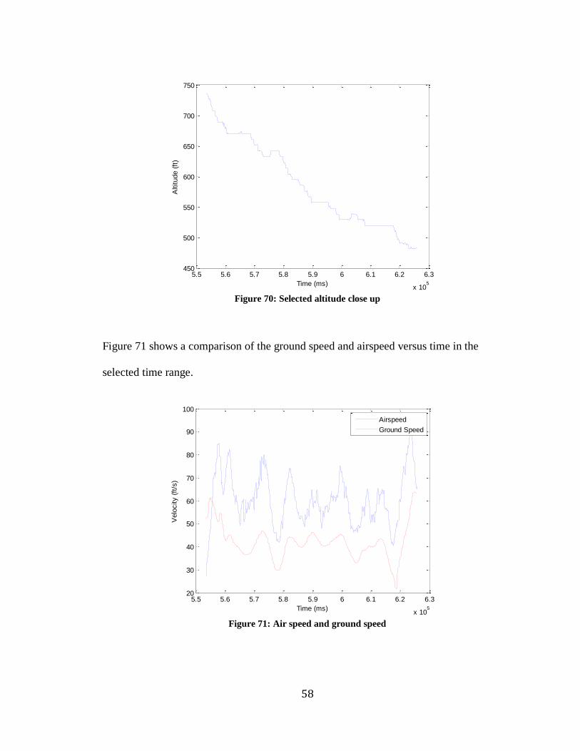
selected altitude that was used to find out the sink rate:

Figure 69: Selected altitude

0 1 2 3 4 5 6 7 8 9 10

x 105

-200

0

200

400

600

800

1000

1200

Time (ms)

Altitude (

ft)

Entire Data Set

Selected Range

58

Figure 70: Selected altitude close up

Figure 71 shows a comparison of the ground speed and airspeed versus time in the

selected time range.

Figure 71: Air speed and ground speed

5.5 5.6 5.7 5.8 5.9 6 6.1 6.2 6.3

x 105

450

500

550

600

650

700

750

Time (ms)

Altitude (

ft)

5.5 5.6 5.7 5.8 5.9 6 6.1 6.2 6.3

x 105

20

30

40

50

60

70

80

90

100

Time (ms)

Velo

city (

ft/s

)

Airspeed

Ground Speed

59

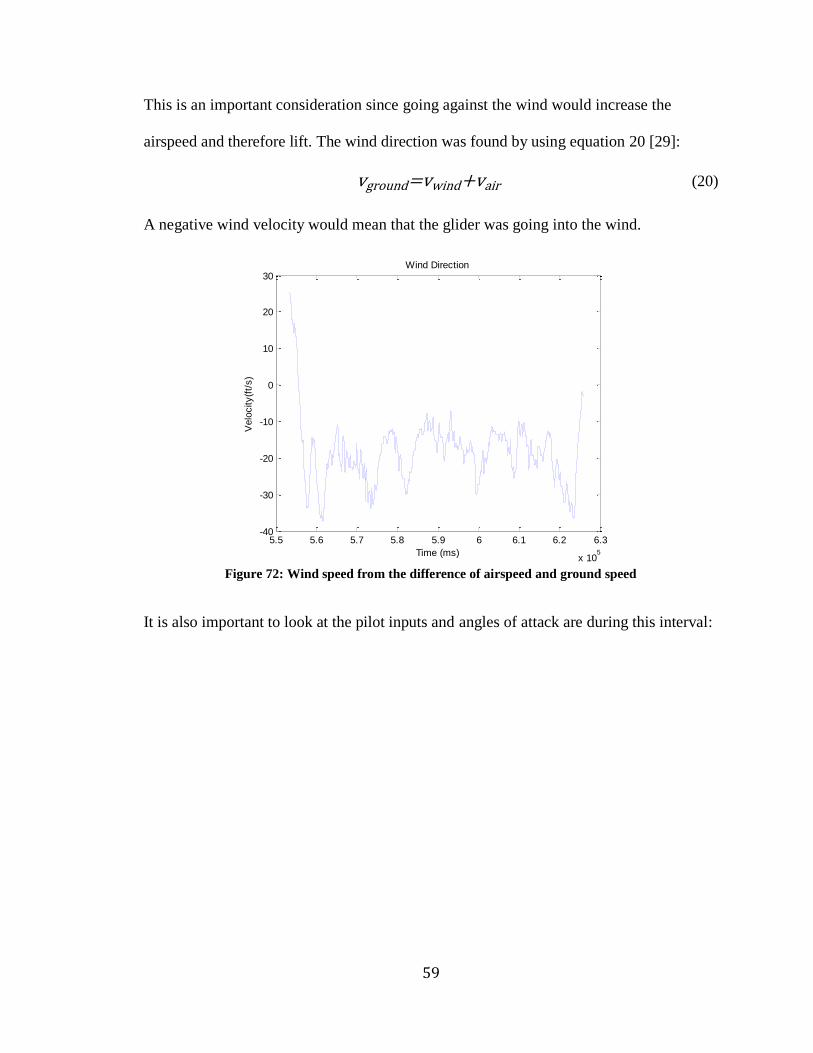
This is an important consideration since going against the wind would increase the

airspeed and therefore lift. The wind direction was found by using equation 20 [29]:

(20)

A negative wind velocity would mean that the glider was going into the wind.

Figure 72: Wind speed from the difference of airspeed and ground speed

It is also important to look at the pilot inputs and angles of attack are during this interval:

5.5 5.6 5.7 5.8 5.9 6 6.1 6.2 6.3

x 105

-40

-30

-20

-10

0

10

20

30

Time (ms)

Velo

city(f

t/s)

Wind Direction

60

Figure 73: Pilot inputs

Figure 74: Measured angle of attack

5.5 5.6 5.7 5.8 5.9 6 6.1 6.2 6.3

x 105

-20

-15

-10

-5

0

5

10

15

Time (ms)

Deflection A

ngle

(deg)

Ch 2 - Elevator Inputs

5.5 5.6 5.7 5.8 5.9 6 6.1 6.2 6.3

x 105

-30

-20

-10

0

10

20

30

Time (ms)

Alp

ha (

deg)

Angle of Attack

61

The glide slope for this glider was found to be 17.233 on April 30th

2014. However, if the

data is taken between 5.8386e5 ms and 6.2388e5 ms, the glide slope is 22.0744. The data

used to find this glide slope is shown in the following graphs:

Figure 75: Selected altitude

Figure 76: Close up of selected altitude range

0 1 2 3 4 5 6 7 8 9 10

x 105

-200

0

200

400

600

800

1000

1200

Time (ms)

Altitude (

ft)

Entire Data Set

Selected Range

5.8 5.85 5.9 5.95 6 6.05 6.1 6.15 6.2 6.25 6.3

x 105

480

500

520

540

560

580

600

Time (ms)

Altitude (

ft)

62

Figure 77:Pilot Inputs

Figure 78: Measured angle of attack

5.8 5.85 5.9 5.95 6 6.05 6.1 6.15 6.2 6.25 6.3

x 105

-20

-15

-10

-5

0

5

10

15

Time (ms)

Deflection A

ngle

(deg)


5.8 5.85 5.9 5.95 6 6.05 6.1 6.15 6.2 6.25 6.3

x 105

-25

-20

-15

-10

-5

0

5

10

15

20

Time (ms)

Alp

ha (

deg)

Angle of Attack

63

Figure 79: Air speed and ground speed comparison

If we compare the two data sets, it becomes clear that the L/D ratio can vary greatly.

Figure 80: Comparison of selected ranges

5.8 5.85 5.9 5.95 6 6.05 6.1 6.15 6.2 6.25 6.3

x 105

20

30

40

50

60

70

80

90

100

Time (ms)

Velo

city (

ft/s

)

Airspeed

Ground Speed

0 1 2 3 4 5 6 7 8 9 10

x 105

-200

0

200

400

600

800

1000

1200

Time (ms)

Altitude

Altitude (

ft)

Entire Data Set

5.5344e5 - 6.2388e5 ms

5.8386e5 - 6.2388e5 ms

64

Figure 81: Comparison of pilot inputs for selected ranges

Figure 82: Comparison of angle of attack among selected ranges

0 1 2 3 4 5 6 7 8 9 10

x 105

-30

-20

-10

0

10

20

30

Time (ms)


Deflection A

ngle

(deg)

Entire Data Set

5.5344e5 - 6.2388e5 ms

5.8386e5 - 6.2388e5 ms

0 1 2 3 4 5 6 7 8 9 10

x 105

-300

-250

-200

-150

-100

-50

0

50

Time (ms)

Angle of Attack

Alp

ha (

deg)

Entire Data Set

5.5344e5 - 6.2388e5 ms

5.8386e5 - 6.2388e5 ms

65

However, this number cannot be used because, due to no accelerometer data in the y-

direction, a constant acceleration due to gravity cannot be assumed. Also, the data up to

this point went through a Butterworth filter to clean out any noise and was generated by

the second script in Appendix G. It should be noted that the filter does alter the numerical

value.

Another method had to be used to figure out the glide slope using the first script

in Appendix G. This included incorporating the error in the barometer and airspeed

sensors. To get the total error from both the barometer and airspeed sensor, equation 22 is

utilized when either multiplying or dividing two numbers with errors [1]:

(21)

(22)

The airspeed sensor was bought from 3DRobotics and had the MPXV7002 Series chip

from Freescale Semiconductor with an error of +/- 6.25% VFSS [18]. The error can be

found by using the given transfer function, equation 23, of the chip located in the data

sheet [18]:

( )) (23)

The Vout was found by using the voltage values from Figure 18 to find the pressure in

kilopascals. Since only a certain range is used within the chip’s operating condition, a

66

ratio can be found by using the difference of pressure used in the actual measurement and

the difference of the total operating range of the chip and then multiplying this number by

6.25% to find an error of +/-0.4074 ft/s [17]. Finding the error for the barometer was

much simpler since it was given in the data sheet for the M5611-01BA03 Barometric

Pressure Sensor from Measurement Specialties [16]. This number is +/- 1.5 mbar, which

converts to +/- 0.0738 in Hg [16]. The error was found by taking the first error free

reading and then subtracting it from the same reading with the error included. This was

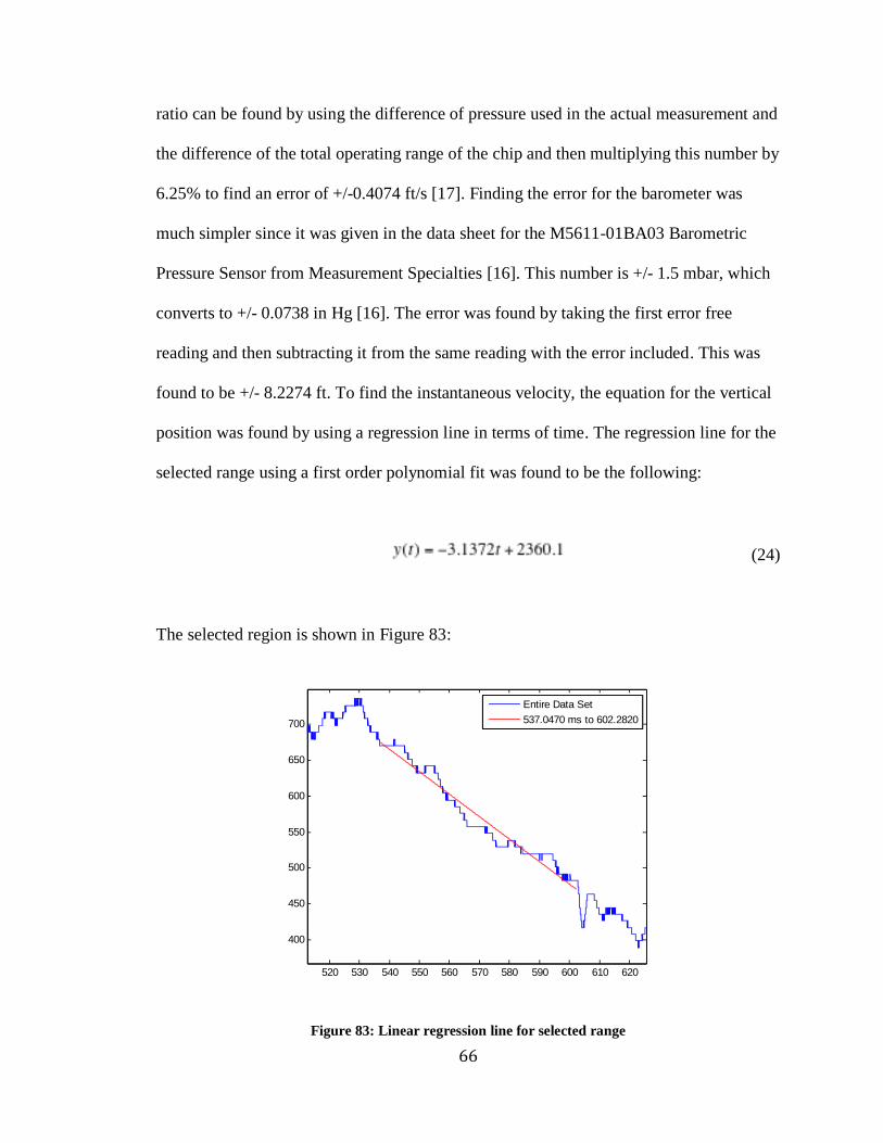
found to be +/- 8.2274 ft. To find the instantaneous velocity, the equation for the vertical

position was found by using a regression line in terms of time. The regression line for the

selected range using a first order polynomial fit was found to be the following:

(24)

The selected region is shown in Figure 83:

Figure 83: Linear regression line for selected range

520 530 540 550 560 570 580 590 600 610 620

400

450

500

550

600

650

700

Entire Data Set

537.0470 ms to 602.2820

67

Taking the derivative gives a constant velocity of -3.1372 ft/s. The first glide

slope ratio data point was found to be 6.9451 using an airspeed of 71.4846 ft/s and a sink

rate of 3.1372 ft/s. An error of 0.2537 ft/s was found for the sink rate by taking the

difference of altitude with the error included and dividing by the time range [15]. This

was the only way to figure out an average error just using the barometer error. The sink

rate is always negative number unless it is being used to calculate the glide slope.

Inserting the information into equation 22 to get equation 25:

z

6.9451

0.4074 ft /s

71.4846 ft /s

0.2537 ft /s

3.1372 ft /s (25)

Solving for z, the error associated with the L/D ratio is +/- 0.7914, which can be shown

in red error bars in Figure 84 for the instantaneous L/D ratio:

Figure 84: Instantaneous L/D with error bars

530 540 550 560 570 580 590 600 61010

15

20

25

30

35

Time (s)

L/D

L/D

Instantaneous L/D

Error

68

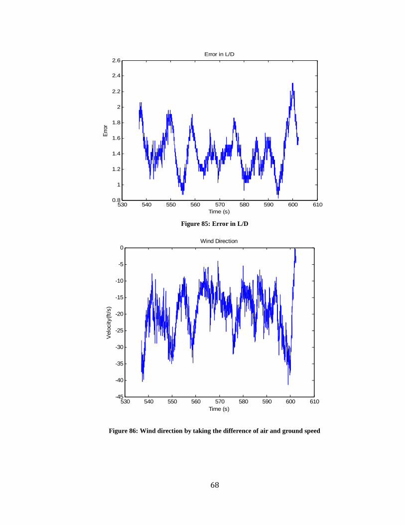
Figure 85: Error in L/D

Figure 86: Wind direction by taking the difference of air and ground speed

530 540 550 560 570 580 590 600 6100.8

1

1.2

1.4

1.6

1.8

2

2.2

2.4

2.6Error in L/D

Err

or

Time (s)

530 540 550 560 570 580 590 600 610-45

-40

-35

-30

-25

-20

-15

-10

-5

0

Time (s)

Velo

city(f

t/s)

Wind Direction

69

However, plotting the residuals show that there is a non-random error as shown in Figure

87. This means that the model chosen, or a polynomial fit order of one, does not fit the

data even though the confidence level is at 95.67% [22].

Figure 87: Residuals to tell how well the linear regression line fits the model

The data was then reanalyzed to the new value for both L/D ratio and a new error. By

increasing the power of the polynomial to two, the average glide slope changes to

21.2520. However, this L/D has a variable error associated with it where the minimum

error is +/- 0.4915 and a maximum of +/- 8.4866.

530 540 550 560 570 580 590 600 610-30

-20

-10

0

10

20

30Residuals

Time (s)

Resid

ual

70

Figure 88: Same selected altitude range but with a 2nd order polynomial fit regression line

Figure 89: Instantaneous L/D with error bars

500 520 540 560 580 600 620

400

450

500

550

600

650

700

750

Entire Data Set

537.0470 ms to 602.2820

530 540 550 560 570 580 590 600 61010

15

20

25

30

35

40

45

50

55

60

Time (s)

L/D

L/D

Instantaneous L/D

Error

71

Figure 90: Error in L/D

Figure 91: Residual plot for the 2nd order polynomial fit regression

530 540 550 560 570 580 590 600 6100

1

2

3

4

5

6

7

8

9Error in L/D

Err

or

Time (s)

530 540 550 560 570 580 590 600 610-30

-20

-10

0

10

20

30Residuals

Time (s)

Resid

ual

72

Nonetheless, a predictive behavior of the residuals, as shown in Figure 91, persists. This

means that the polynomial fit chosen still does not fit and that a variable has not be

accounted for [22].

The average glide slope was found to be between 19.1617 for a polynomial fit order

of one and 21.2520 for an order of two. However, the average errors associated with both

glide slopes need to be found by using the rules for addition as shown in equations 26 and

27 [1]:

(26)

(27)

The average glide slopes become 21.2520 +/- 1.99 and 19.1617 +/- 1.4196.

73

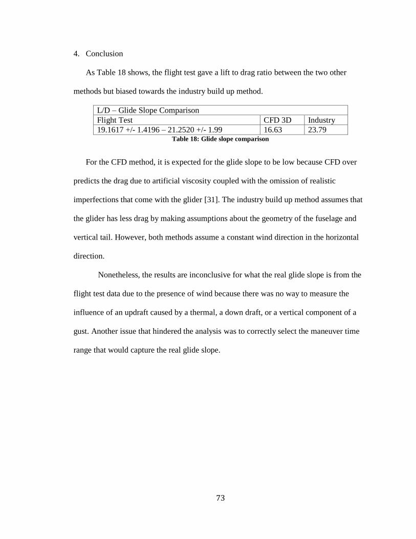
4. Conclusion

As Table 18 shows, the flight test gave a lift to drag ratio between the two other

methods but biased towards the industry build up method.

L/D – Glide Slope Comparison

Flight Test CFD 3D Industry

19.1617 +/- 1.4196 – 21.2520 +/- 1.99 16.63 23.79 Table 18: Glide slope comparison

For the CFD method, it is expected for the glide slope to be low because CFD over

predicts the drag due to artificial viscosity coupled with the omission of realistic

imperfections that come with the glider [31]. The industry build up method assumes that

the glider has less drag by making assumptions about the geometry of the fuselage and

vertical tail. However, both methods assume a constant wind direction in the horizontal

direction.

Nonetheless, the results are inconclusive for what the real glide slope is from the

flight test data due to the presence of wind because there was no way to measure the

influence of an updraft caused by a thermal, a down draft, or a vertical component of a

gust. Another issue that hindered the analysis was to correctly select the maneuver time

range that would capture the real glide slope.

74

5. Future Work

There are many things to improve upon within this project. The most important issue

is to upgrade and add more instrumentation to get an accurate measurement of the glide

slope. Some suggestions for new instrumentation, but not a complete list, would include

the following:

Variometer

The variometer is an important piece since it measures the rate of descent or

ascent. This will give an instantaneous measurement of the vertical velocity so

that a polynomial fit would not have to be used. This sensor coupled with a

ground station would make finding thermals easy to keep aloft for longer periods.

This would help in figuring out the speed polar for the glider [27]. A digital

variometer could be implemented using a complimentary filter to fuse the

barometric vertical velocity and vertical acceleration readings [38].

Real-time telemetry sent to pilot

It was difficult to make sure that the glider was flying level from the ground until

the data was analyzed. Knowing the angle of attack in real time or having

autopilot would save a lot of time instead of analyzing the angle of attack data

after landing. This would also allow testing of the L/D at different angles of

attack.

Strain gauges or accelerometers to measure the wing deflection

By knowing the instantaneous deflection of the wings, a deeper understanding of

its dynamics and design can be examined [26]. One important dynamic behavior

to avoid is when does fluttering occur.

75

Better air data boom

A redesign of the air data boom structure is needed because time is wasted when

recalibrating when the potentiometers for the AoA and AoY vanes are replaced.

The design needs to incorporate a holder so that the potentiometer could be

placed in a more accessible position. Also, designing a wing with a place where

the boom could be threaded in using a threaded rod and access point would

improve the measurements and any logistical issues. A wind tunnel test should be

done to determine the size of the vanes to improve the measurements for AoA

and AoY.

Inertia

A contraption will have to be built so that a scale glider could swing and the

inertias found by using the swing method [20].

Motor Testing

A new test should be done to look at the efficiency of different blade

configurations and throttle position.

76

References

[1] Linberg, Vern. Uncertainties and Error Propagation. Part I of a manual on

Uncertainties, Graphing, and the Vernier Caliper. RIT, 1 July 2000. Web. 21

June 2014.

[2] Alvydas Civinskas (student) in discussion with professor Moncayo, January 2014.

[3] McClanahan, Jade. Numerical Evaluation of Glider Aerodynamic Performance.

[4] Mckee, Kyle. “Novel Airframe Design for the Dual-Aircraft Atmospheric Platform

Flight Concept. MS Thesis.” Embry Riddle Aeronautical University, 2012. Print.

[5] “AVL” MIT. MIT. N.d, n.p. Web.<http://web.mit.edu/drela/Public/web/avl/>

[6] “GL04 - Ka-8b ELECTRIC 6000 ARF 1/2.5 SCALE." Phoenix Model. Phoenix

Model, n.d. Web. Jan. 2014.

<http://phoenixmodel.com/Product.aspx?ProductId=295>.

[7] “Barometric Formula” Hyperphuysics. Georgia State University, n.d., n.p. Web. 17

June 2014. <http://hyperphysics.phy-astr.gsu.edu/hbase/kinetic/barfor.html>

[8] Federal Aviation Administration. Chapter 3: Aerodynamics of Flight. FAA. PDF File.

[9]"HQ 3.0/15 AIRFOIL." Airfoil Tools. N.p., n.d. Web. Jan. 2014.

<http://airfoiltools.com/airfoil/details?airfoil=hq3015-il>.

[10] "Lift & Drag Polars." Airfoil Tools. N.p., n.d. Web. Jan. 2014.

<http://airfoiltools.com/airfoil/details?r=polar/index/#xfoil>.

[11] Drela, Mark. "Xfoil - Subsonic Airfoil Development System." MIT. MIT, 11 Dec.

2000. Web. <http://web.mit.edu/drela/Public/web/xfoil/>.

[12] Coxworth, Ben. Solar-powered UAV could fly in the upper atmosphere for 5

years at a time. Gizmag. Web. 20 June 2014.

<http://www.gizmag.com/solara-uav-atmospheric-satellite/28886/>

[13] Chapman, Matthew. Facebook buys UK-based drone company Ascenta to ‘beam’

internet from sky. Marketing Magazine. Web. 20 June 2014.

<http://www.marketingmagazine.co.uk/article/1287644/facebook-buys-

uk-based-drone-company-ascenta-beam-internet-sky>

[14] Quick, Darren. Lockheed Martin’s HALE-D airship takes to the air. Gizmag. Web.

20 June 2014. <http://www.gizmag.com/lockheed-martin-hale-d-airship/19360/>

http://www.gizmag.com/solara-uav-atmospheric-satellite/28886/

http://www.gizmag.com/lockheed-martin-hale-d-airship/19360/

77

[15] Error Analysis. University of Tennessee of Martin. N.d., n.p. Web.

<http://www.utm.edu/staff/cerkal/Lect4.html>

[16] Measurement Specialties. MS5611-01BA03 Barometric Pressure Sensor, with

stainless steel cap. Measurement Specialties. PDF File.

[17] Honeywell. Pressure Transducer Accuracy in Application. Honeywell. PDF File.

[18] Freescale Semiconductor, Inc. MPXV7002 Series. Freescale Semiconductor, Inc.

PDF File.

[19] Longacre. Computerscales Accuset II Basic System. N.d., Longacre. Web.

<http://www.longacreracing.com/products.aspx?prodid=7143>

[20] Watkiss, Eric John. Flight Dynamics of an Unmanned Aerial Vehicle Monterey,

CA: US Naval Postgraduate School. 1994. PDF File.

[21] National Institute of Standards and Technology. Are the model residuals well-

behaved? N.d., NIST. Web.

<http://www.itl.nist.gov/div898/handbook/pri/section2/pri24.htm>

[22] Phoenix Model. Instruction Manual: K8B. Print.

[23] Alvydas Civinskas (student) in discussion with professor Moncayo, June 2014

[24] Thompson, David E. “Harmonic Response of Second Order Systems” University of

Idaho, 2006., n.p. Web. 30 June 2014.

<http://www.engr.uidaho.edu/thompson/courses/ME330/lecture/SecondOrderSyst

ems.html>

[25] “Aircraft Center of Gravity Calculator” n.p.

Web. 5 Julty 2014. <http://adamone.rchomepage.com/cg_calc.htm>

[26] Qiao, Yuqing. “Effect of Wing Flexibility on Aircraft Flight Dynamics.” MA

Thesis. Cranfield University, 2012. Web. 9 July 2014.

[27] Federal Aviation Administration. Chapter 5: Glider Performance. FAA. PDF File.

[28] Engblom, William A. “Development of an Atmospheric Satellite Concept Based on

Sailing.” AIAA SciTech: 52nd

Aerospace meeting. National Harbor, Maryland 13-

14 January 2014. n.p.

[29] Ohlson, Dawn. The Mathematics of Aircraft Navigation. Royal Academy of

Engineering. n.d. PDF File.

[30] Alvydas Civinskas (student) in discussion with professor Engblom, July 2014.

http://www.utm.edu/staff/cerkal/Lect4.html

http://www.itl.nist.gov/div898/handbook/pri/section2/pri24.htm

http://adamone.rchomepage.com/cg_calc.htm

78

[31] Espritmodel Sailplane Takeoff Dolly 1/3 Scale.Web.

<http://www.espritmodel.com/sailplane-takeoff-dolly-1-3-scale.aspx>.

[31] Virginia Tech. Performance. Virginia Tech. PDF File.

[33] Federal Aviation Administration. Chapter 7: Launch and Recovery Procedures and

Flight Maneuvers. FAA. PDF File.

[34] International Civil Aviation Organization. Study Note 2, Appendix, Checklist of

AMD 37 Revisions 2014. Microsoft Word file

[35] “Phoenix Models K8b – 3.5m ARFT” Hyperflight UK. Hyperflight UK. n.d. Web.

Aug 2014.

<http://www.hyperflight.co.uk/products.asp?code=PM%2DK8B%2D3M>

[36] Alvydas Civinskas (student) in discussion with professor Moncayo, August 2014

[37] Alvydas Civinskas (student) in discussion with professor Engblom, June 2014

[38] Higgins, Jr., Walter T. “A Comparison of Complementary and Kalman Filtering.”

IEEE Transactions on Aerospace and Electronic Systems. 3 (1975): 321-325.

Web.

[39] Fatica, Massimiliano and Antony Jameson. Using Computational Fluid Dynamics

for Aerodynamics. Stanford University. PDF File.

[40] Yechout, Thomas R., Steven L. Morris, David E. Bossert, and Wayne F. Hallgren.

Introduction to Aircraft Flight Mechanics: Performance, Static Stability, Dynamic

Stability, and Classical Feedback Control. Reston, VA:American Institute of

Aeronautics and Astronautics, Inc. 2003.

[41] MEDIATEK. MEDIATEK-3329 Datasheet. MEDIATEK. PDF File.

[42] Zuo, Wangda. Introduction of Computational Fluid Dynamics.

[43] Alvydas Civinskas (student) in discussion with Daniel Harrison (RC pilot), June

2014

79

Appendix:

A. Flight Test Data

a. April 30th

2014

0 1 2 3 4 5 6 7 8 9 10

x 105

800

1000

1200

1400

1600

1800

2000

2200Ch4 - Left Aileron

Time (ms)

80

0 1 2 3 4 5 6 7 8 9 10

x 105

1000

1200

1400

1600

1800

2000

2200Ch3 - Rudder

Time (ms)

0 1 2 3 4 5 6 7 8 9 10

x 105

1000

1100

1200

1300

1400

1500

1600

1700

1800

1900

2000Ch2 - Elevator

Time (ms)

81

0 1 2 3 4 5 6 7 8 9 10

x 105

800

1000

1200

1400

1600

1800

2000

2200Ch1 - Right Aileron

Time (ms)

0 1 2 3 4 5 6 7 8 9 10

x 105

-10

0

10

20

30

40

50

60

70

80

90Airspeed

mph

Time (ms)

82

0 1 2 3 4 5 6 7 8 9 10

x 105

-30

-20

-10

0

10

20

30

40

50

60Beta

deg

Time (ms)

0 1 2 3 4 5 6 7 8 9 10

x 105

-300

-250

-200

-150

-100

-50

0

50Alpha

deg

Time (ms)

83

0 1 2 3 4 5 6 7 8 9 10

x 105

0

50

100

150

200

250

300

350

400Altitude

m

Time (ms)

0 1 2 3 4 5 6 7 8 9 10

x 105

-2

-1.5

-1

-0.5

0

0.5

1

1.5

2phi

deg

Time (ms)

84

0 1 2 3 4 5 6 7 8 9 10

x 105

-1.5

-1

-0.5

0

0.5

1

1.5

2theta

deg

Time (ms)

0 1 2 3 4 5 6 7 8 9 10

x 105

-400

-300

-200

-100

0

100

200

300

400r

deg/s

Time (ms)

85

0 1 2 3 4 5 6 7 8 9 10

x 105

-500

-400

-300

-200

-100

0

100

200

300

400q

deg/s

Time (ms)

0 1 2 3 4 5 6 7 8 9 10

x 105

-400

-300

-200

-100

0

100

200

300

400p

deg/s

Time (ms)

86

b. May 8

th 2014 – 1

0 1 2 3 4 5 6 7 8 9 10

x 105

0

10

20

30

40

50

60

70

80Ground Speed

ft/s

Time (ms)

0 1 2 3 4 5 6 7

x 105

0

500

1000

1500

2000


Time (ms)

87

0 1 2 3 4 5 6 7

x 105

0

500

1000

1500

2000

2500Ch3 - Rudder

Time (ms)

0 1 2 3 4 5 6 7

x 105

0

200

400

600

800

1000

1200

1400

1600

1800

2000Ch2 - Elevator

Time (ms)

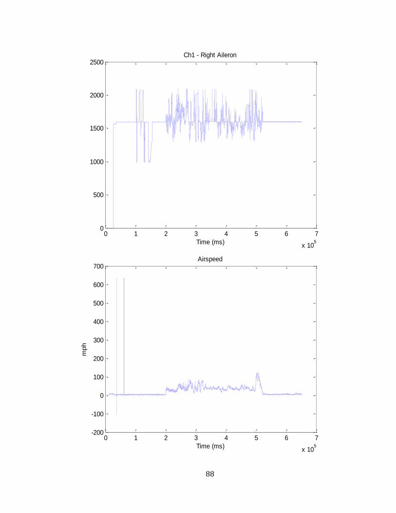
88

0 1 2 3 4 5 6 7

x 105

0

500

1000

1500

2000


Time (ms)

0 1 2 3 4 5 6 7

x 105

-200

-100

0

100

200

300

400

500

600

700Airspeed

mph

Time (ms)

89

0 1 2 3 4 5 6 7

x 105

-10

-5

0

5

10

15

20

25

30

35

40Beta

deg

Time (ms)

0 1 2 3 4 5 6 7

x 105

-300

-250

-200

-150

-100

-50

0Alpha

deg

Time (ms)

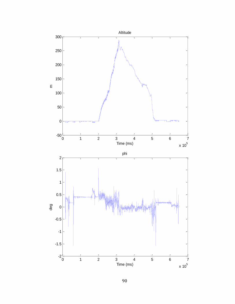
90

0 1 2 3 4 5 6 7

x 105

-50

0

50

100

150

200

250

300Altitude

m

Time (ms)

0 1 2 3 4 5 6 7

x 105

-2

-1.5

-1

-0.5

0

0.5

1

1.5

2phi

deg

Time (ms)

91

0 1 2 3 4 5 6 7

x 105

-2

-1.5

-1

-0.5

0

0.5

1

1.5

2theta

deg

Time (ms)

0 1 2 3 4 5 6 7

x 105

-300

-200

-100

0

100

200

300

400

500r

deg/s

Time (ms)

92

0 1 2 3 4 5 6 7

x 105

-400

-300

-200

-100

0

100

200

300

400

500q

deg/s

Time (ms)

0 1 2 3 4 5 6 7

x 105

-400

-300

-200

-100

0

100

200

300

400p

deg/s

Time (ms)

93

c. May 8

th 2014 – 2

0 1 2 3 4 5 6 7

x 105

0

10

20

30

40

50

60

70

80Ground Speed

ft/s

Time (ms)

0 1 2 3 4 5 6 7 8 9 10

x 105

0

500

1000

1500

2000


Time (ms)

94

0 1 2 3 4 5 6 7 8 9 10

x 105

0

500

1000

1500

2000

2500Ch3 - Rudder

Time (ms)

0 1 2 3 4 5 6 7 8 9 10

x 105

0

200

400

600

800

1000

1200

1400

1600

1800

2000Ch2 - Elevator

Time (ms)

95

0 1 2 3 4 5 6 7 8 9 10

x 105

0

500

1000

1500

2000


Time (ms)

0 1 2 3 4 5 6 7 8 9 10

x 105

-20

0

20

40

60

80

100

120Airspeed

mph

Time (ms)

96

0 1 2 3 4 5 6 7 8 9 10

x 105

-20

-10

0

10

20

30

40

50

60Beta

deg

Time (ms)

0 1 2 3 4 5 6 7 8 9 10

x 105

-280

-260

-240

-220

-200

-180

-160

-140

-120

-100

-80Alpha

deg

Time (ms)

97

0 1 2 3 4 5 6 7 8 9 10

x 105

-100

0

100

200

300

400

500

600Altitude

m

Time (ms)

0 1 2 3 4 5 6 7 8 9 10

x 105

0

20

40

60

80

100

120Ground Speed

ft/s

Time (ms)

98

0 1 2 3 4 5 6 7 8 9 10

x 105

-2

-1.5

-1

-0.5

0

0.5

1

1.5

2phi

deg

Time (ms)

0 1 2 3 4 5 6 7 8 9 10

x 105

-1.5

-1

-0.5

0

0.5

1

1.5

2theta

deg

Time (ms)

99

0 1 2 3 4 5 6 7 8 9 10

x 105

-200

-150

-100

-50

0

50

100

150

200

250

300r

deg/s

Time (ms)

0 1 2 3 4 5 6 7 8 9 10

x 105

-300

-200

-100

0

100

200

300q

deg/s

Time (ms)

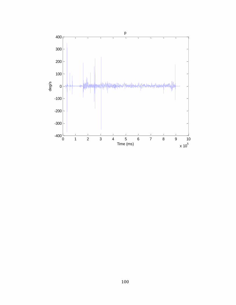
100

0 1 2 3 4 5 6 7 8 9 10

x 105

-400

-300

-200

-100

0

100

200

300

400p

deg/s

Time (ms)

101

B. DATCOM Graphs

-2 0 2 4 6 8 10

0.04

0.045

0.05

0.055

0.06

0.065

0.07

CD

vs.

(deg)

CD

WBHV

Mach = 0.100

Alt = 300 feet

WBHV Cdo =

0.021

-2 0 2 4 6 8 10

0.9

1

1.1

1.2

1.3

1.4

CL vs.

(deg)

CL

WBHV

Mach = 0.100

Alt = 300 feetWBHV C

L0 =

0.999

102

-2 0 2 4 6 8 10-0.9

-0.8

-0.7

-0.6

-0.5

-0.4

-0.3

-0.2

-0.1

0

0.1

Cm

vs.

(deg)

Cm

WBHV

Mach = 0.100

Alt = 300 feetWBHV C

m0 =

-0.090

-2 0 2 4 6 8 100.8

0.9

1

1.1

1.2

1.3

1.4

CN vs.

(deg)

CN

WBHV

Mach = 0.100

Alt = 300 feet

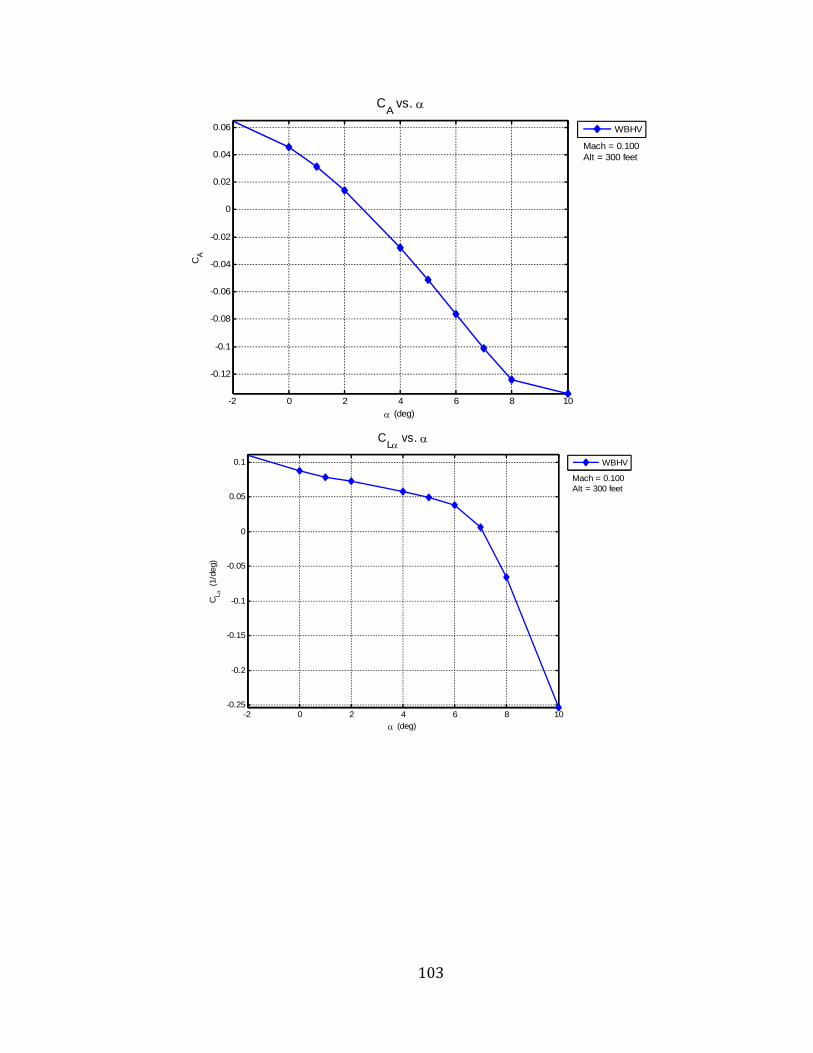
103

-2 0 2 4 6 8 10

-0.12

-0.1

-0.08

-0.06

-0.04

-0.02

0

0.02

0.04

0.06

CA vs.

(deg)

CA

WBHV

Mach = 0.100

Alt = 300 feet

-2 0 2 4 6 8 10-0.25

-0.2

-0.15

-0.1

-0.05

0

0.05

0.1

CL

vs.

(deg)

CL (

1/d

eg)

WBHV

Mach = 0.100

Alt = 300 feet

104

-2 0 2 4 6 8 10

-3.8

-3.7

-3.6

-3.5

-3.4

-3.3

-3.2

-3.1

-3

x 10-4

Cl

vs.

(deg)

Cl

(1/d

eg)

WBHV

Mach = 0.100

Alt = 300 feet

-0.15 -0.1 -0.05 0 0.05 0.10.7

0.8

0.9

1

1.1

1.2

1.3

1.4

1.5

CN vs. C

A

CA

CN

WBHV

Mach = 0.100

Alt = 300 feet

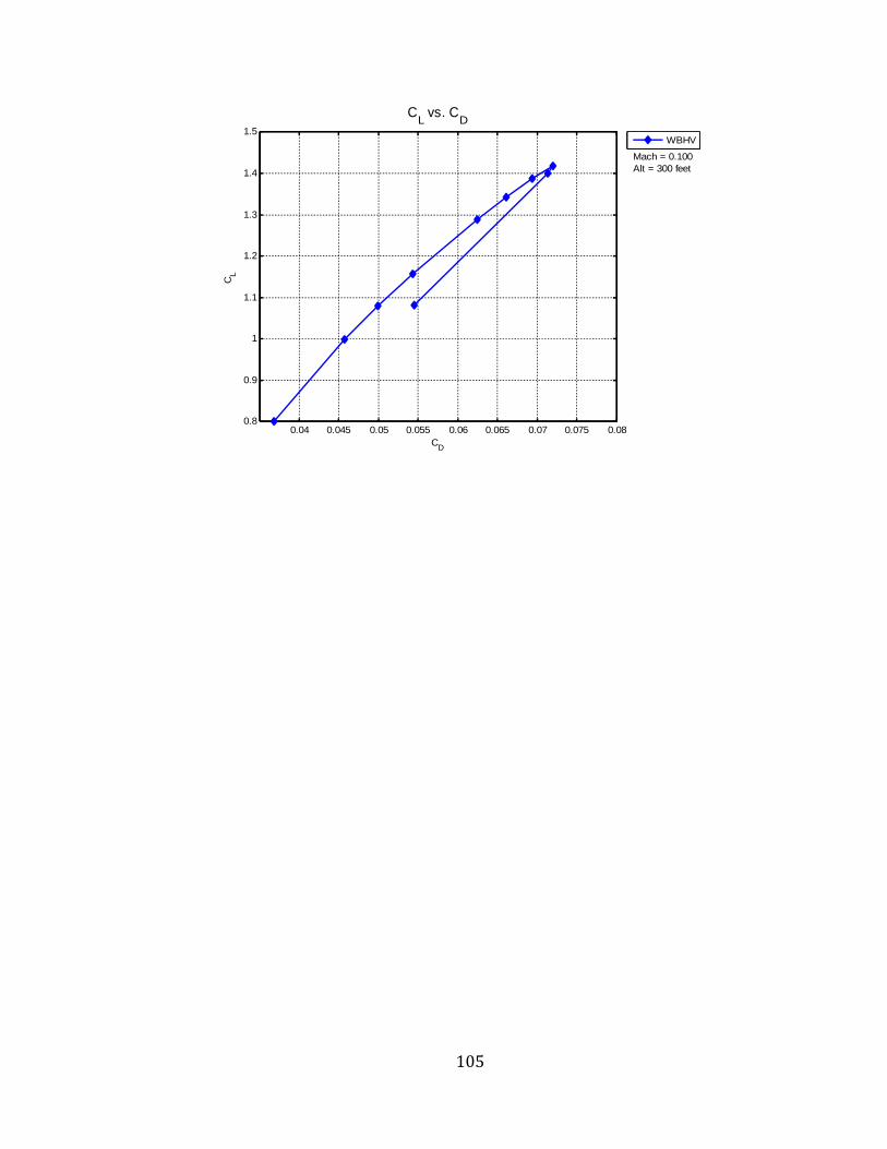
105

0.04 0.045 0.05 0.055 0.06 0.065 0.07 0.075 0.080.8

0.9

1

1.1

1.2

1.3

1.4

1.5

CL vs. C

D

CD

CL

WBHV

Mach = 0.100

Alt = 300 feet

106

C. Pilot Inputs

a. Flight Test on April 30th

2014

y = 0.0687x - 113.74

-30

-20

-10

0

10

20

30

40

900 1400 1900 2400

De

fle

ctio

n A

ng

le (

de

g)

Output Signal

Ch 1 Aileron

Series1

Linear (Series1)

y = 0.0577x - 84.46

-20

-10

0

10

20

30

40

900 1100 1300 1500 1700 1900 2100De

fle

ctio

n A

ng

le (

de

g)

Output Signal

Ch 2 Elevator

Series1

Linear (Series1)

107

b. Flight Test on May 8th

2014 - 1

y = 0.0423x - 60.958

-30

-20

-10

0

10

20

30

40

900 1400 1900 2400

De

fle

ctio

n A

ng

le (

de

g)

Output Signal

Ch 3 Rudder

Series1

Linear (Series1)

y = 0.0504x - 77.99

-40

-30

-20

-10

0

10

20

30

40

900 1400 1900 2400

De

fle

ctio

n A

ng

le (

de

g)

Output Signal

Ch 1 Aileron

Series1

Linear (Series1)

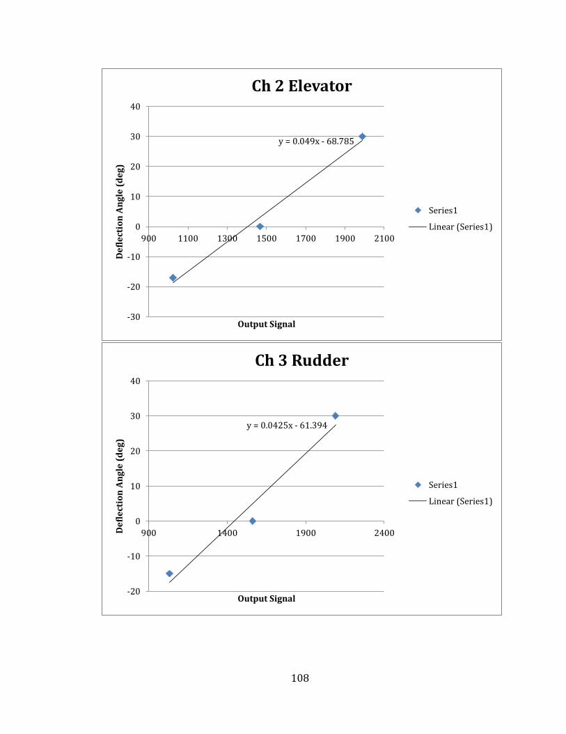
108

y = 0.049x - 68.785

-30

-20

-10

0

10

20

30

40

900 1100 1300 1500 1700 1900 2100

De

fle

ctio

n A

ng

le (

de

g)

Output Signal

Ch 2 Elevator

Series1

Linear (Series1)

y = 0.0425x - 61.394

-20

-10

0

10

20

30

40

900 1400 1900 2400De

fle

ctio

n A

ng

le (

de

g)

Output Signal

Ch 3 Rudder

Series1

Linear (Series1)

109

c. Flight Test on May 8th

2014 - 2

y = 0.0687x - 113.66

-30

-20

-10

0

10

20

30

40

900 1400 1900 2400

De

fle

ctio

n A

ng

le (

de

g)

Output Signal

Ch 1 Aileron

Series1

Linear (Series1)

y = 0.0579x - 84.913

-20

-10

0

10

20

30

40

900 1100 1300 1500 1700 1900 2100De

fle

ctio

n A

ng

le (

de

g)

Output Signal

Ch 2 Elevator

Series1

Linear (Series1)

110

y = 0.0425x - 60.97

-20

-10

0

10

20

30

40

900 1400 1900 2400De

fle

ctio

n A

Ng

le (

de

g)

Output Signal

Ch 3 Rudder

Series1

Linear (Series1)

111

D. Graphs for Simulink Model

a. Stability Derivatives

Stability coefficient Value Unit

CL0 0.28

CLa 5.65112 1/rad

CLq 7.5 1/rad

CLde 0.22735 1/rad

CLih 0

CD0 0.0164

CDa 0.37442 1/rad

CDde -0.00462 1/rad

CDih 0

CDq 0

Cm0 0.048

Cma -.47318 1/rad

Cmq -16.47972 1/rad/s

Cmde -1.26278 1/rad

Cmih 0

Cl0 0

Clb -0.9 1/rad

Clp -0.65596 1/rad/s

Clr 0.18415 1/rad/s

Clda -3.96308 1/rad

Cldr 0.39041 1/rad

Cn0 0

Cnb 0.04641 1/rad

Cnp -0.04016 1/rad/s

Cnr 0.03587 1/rad/s

Cnde 0.00462 1/rad

Cnda 0.40969 1/rad

Cndr 0.32189 1.rad

CY0 0

CYb -0.2595 1/rad

CYda 2.22584 1/rad

CYp 0.0075

Cyr 0.146

CYdr -1.17913 1/rad

112

b. Trimmed Model Graphs

0 20 40 60 80 100 120 140 160 180

160

165

170

175

180

Altitude

Altitude (

m)

Time (s)

0 50 100 150 200 250 300 3505

10

15

20

Airspeed

Airspeed (

m/s

)

Time (s)

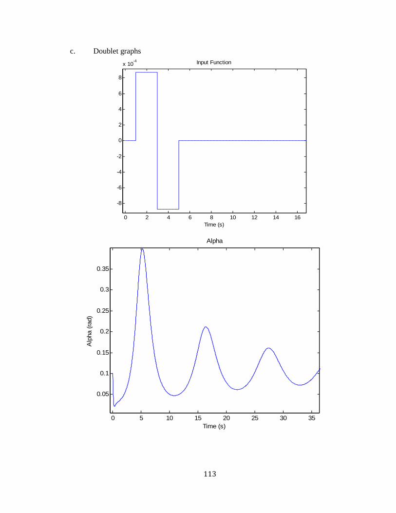
113

c. Doublet graphs

0 2 4 6 8 10 12 14 16

-8

-6

-4

-2

0

2

4

6

8

x 10-4 Input Function

Time (s)

0 5 10 15 20 25 30 35

0.05

0.1

0.15

0.2

0.25

0.3

0.35

Alpha

Alp

ha (

rad)

Time (s)

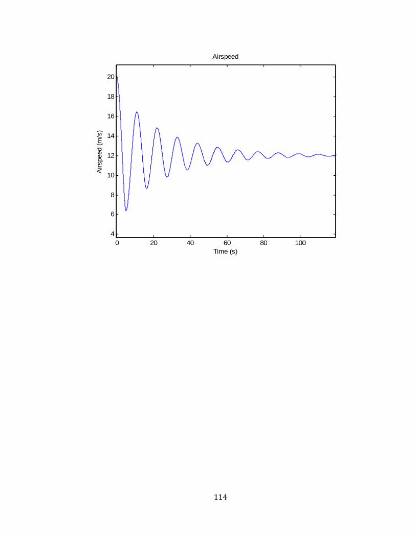
114

0 20 40 60 80 100

4

6

8

10

12

14

16

18

20

Airspeed

Airspeed (

m/s

)

Time (s)

115

E. Optimization

Iteration

F-

count

alpha

(min) beta (min) p (min) q (min) r (min) theta (min) phi (min)

0 1 3.52E+03 233.2719 96.7276 452.8464 120.5737 6.55E+06 319.5111

1 26 8.80E+03 1.90E+03 1.51E+03 3.09E+03 1.31E+05 6.54E+05 5.17E+06

2 29 1.11E+03 4.33E+03 3.94E+03 210.9835 2.77E+04 1.49E+06 2.13E+06

3 32 5.10E+03 1.28E+04 172.6951 1.11E+03 4.56E+04 2.45E+05 2.61E+06

4 36 5.09E+03 1.28E+04 171.3497 1.12E+03 4.58E+04 2.30E+05 2.55E+06

5 40 5.08E+03 1.27E+04 170.1352 1.12E+03 4.63E+04 2.10E+05 2.46E+06

6 53 5.08E+03 1.27E+04 170.1676 1.12E+03 4.62E+04 2.10E+05 2.46E+06

7 66 5.07E+03 1.27E+04 170.2327 1.12E+03 4.62E+04 2.10E+05 2.45E+06

8 79 5.06E+03 1.27E+04 170.7596 1.12E+03 4.62E+04 2.11E+05 2.45E+06

9 92 4.97E+03 1.24E+04 175.3959 1.07E+03 4.61E+04 2.16E+05 2.41E+06

10 124 4.94E+03 1.23E+04 174.4054 1.07E+03 4.59E+04 2.04E+05 2.35E+06

11 156 4.93E+03 1.23E+04 174.4729 1.07E+03 4.57E+04 2.04E+05 2.32E+06

12 214 4.93E+03 1.23E+04 174.4729 1.07E+03 4.57E+04 2.04E+05 2.32E+06

13 272 4.93E+03 1.23E+04 174.4729 1.07E+03 4.57E+04 2.04E+05 2.32E+06

14 330 4.93E+03 1.23E+04 174.4729 1.07E+03 4.57E+04 2.04E+05 2.32E+06

15 388 4.93E+03 1.23E+04 174.4729 1.07E+03 4.57E+04 2.04E+05 2.32E+06

16 402 3.01E+03 5.42E+03 276.9322 365.2483 4.53E+04 1.81E+05 1.16E+06

17 460 3.01E+03 5.42E+03 276.9322 365.2483 4.53E+04 1.81E+05 1.16E+06

18 467 2.85E+03 5.41E+03 267.7889 371.9185 4.55E+04 9.51E+04 8.49E+05

19 525 2.85E+03 5.41E+03 267.7889 371.9185 4.55E+04 9.51E+04 8.49E+05

20 583 2.85E+03 5.41E+03 267.7889 371.9185 4.55E+04 9.51E+04 8.49E+05

21 641 2.85E+03 5.41E+03 267.7889 371.9185 4.55E+04 9.51E+04 8.49E+05

22 699 2.85E+03 5.41E+03 267.7889 371.9185 4.55E+04 9.51E+04 8.49E+05

23 757 2.85E+03 5.41E+03 267.7889 371.9185 4.55E+04 9.51E+04 8.49E+05

24 761 2.86E+03 5.37E+03 265.175 368.6721 4.55E+04 8.43E+04 8.16E+05

25 819 2.86E+03 5.37E+03 265.175 368.6721 4.55E+04 8.43E+04 8.16E+05

26 848 2.87E+03 5.37E+03 261.9004 364.4361 4.59E+04 7.93E+04 7.99E+05

27 906 2.87E+03 5.37E+03 261.9004 364.4361 4.59E+04 7.93E+04 7.99E+05

28 965 2.87E+03 5.37E+03 261.9004 364.4361 4.59E+04 7.93E+04 7.99E+05

29 1003 2.83E+03 5.45E+03 261.2299 364.7912 4.57E+04 7.76E+04 7.96E+05

30 1062 2.83E+03 5.45E+03 261.2299 364.7912 4.57E+04 7.76E+04 7.96E+05

31 1122 4.54E+03 6.98E+03 9.41E+03 1.33E+04 9.13E+04 2.35E+07 4.12E+10

32 1182 4.54E+03 6.98E+03 9.41E+03 1.33E+04 9.13E+04 2.35E+07 4.12E+10

33 1242 4.54E+03 6.98E+03 9.41E+03 1.33E+04 9.13E+04 2.35E+07 4.12E+10

34 1302 4.54E+03 6.98E+03 9.41E+03 1.33E+04 9.13E+04 2.35E+07 4.12E+10

35 1362 4.54E+03 6.98E+03 9.41E+03 1.33E+04 9.13E+04 2.35E+07 4.12E+10

36 1422 4.54E+03 6.98E+03 9.41E+03 1.33E+04 9.13E+04 2.35E+07 4.12E+10

37 1482 4.54E+03 6.98E+03 9.41E+03 1.33E+04 9.13E+04 2.35E+07 4.12E+10

38 1542 4.54E+03 6.98E+03 9.41E+03 1.33E+04 9.13E+04 2.35E+07 4.12E+10

39 1602 4.54E+03 6.98E+03 9.41E+03 1.33E+04 9.13E+04 2.35E+07 4.12E+10

116

F. Stability Derivatives Comparison

Stability

Characteristic Variable Flight Testing Surfaces (deg)

Datcom

(deg) AVL (deg)

Lift coefficient CL 1.18 0.999 1.12

Lift curve slope CLa 0.0978 0.0872 0.1125

Lifr curve

variation wrt AoY CLb 0 0 0

Lift variation wrt p CLp -0.000162 0 0

Lift variation wrt q CLq 0.121 0 0.23975

Lift variation wrt r CLr 0 0 0

Drag coefficient CD0 .046 0.046 .02235

Drag coefficient

slope CDa 0.00673 0 0

Drag variation wrt

p CDp 0 0 0

Drag variation wrt

q CDq 0.00444 0 0

Drag variation wrt

r CDr 0 0 0

Basic pitching

moment Cm0 0 -0.0898 -0.2659

Pitching moment

wrt AoA Cma -0.00111 -0.1137 -0.0526

Pitching moment

wrt AoY Cmb 0 0 0

Pitching moment

wrt p Cmp 0 0 0

Pitching moment

wrt q Cmq -0.280 0 -0.3971

Pitching moment

wrt r Cmr 0 0 0

Basic rolling

moment Cl0 0 0 0

Rolling moment

wrt AoA Cla 0 0 0

Dihedral effect Clb -0.000116 -3.587E-04 -0.00104

Damping-in-Roll

derivative Clp -0.0113 0 -0.01243

Rolling moment

wrt q Clq 0 0 0

Cross derivative

due to yaw Clr 0.00318 0 -0.005066

Basic yawing

moment Cn0 0 0.999 0

117

Yawing moment wrt AoA Cna 0 0 0

Directional

stability Cnb 0.000772 2.988E-04 0.001048

Cross derivative

due to roll Cnp -0.000683 0 -0.001825

Yawing moment

wrt q Cnq 0 0 0

Damping-in-Yaw

derivative Cnr -0.000596 0 -0.001129

FY Cy0 0 0 0

FY variation wrt

to AoA Cya 0 0 0

Side force

derivative Cyb -0.00447 -0.00296 -0.004743

Side force due to

roll derivative Cyp 0.000107 0 -7.565eE4

FY variation wrt

to q Cyq 0 0 0

FY variation wrt

to r Cyr 0.00247 0 0.003886

Aileron

Lift variation with

roll Clda -0.00112 0 0.011842

Drag variation

with roll CDda 0 0 0

FFY variation in

roll Cyda 0.000220

0

0.001426

MX variation in

roll Clda -0.00643

0

0.011631

MY variation in

roll Cmda -0.000617

0

-0.003549

MZ variation in

roll Cnda 0.000530

0

-0.000237

Elevator

Lift variation with

pitch Clde 0.00721

0

0.008957

Drag variation

with pitch CDde 0.000273

0

0

FY variation in

pitch Cyde 0

0

0

MX variation in

pitch Clde 0

0

0

MY variation in

pitch Cmde -0.0263

0

-0.035863

MZ variation in Cnde 0 0 0

118

pitch

Rudder (left)

Lift variation with

yaw CLdr -0.0000318

0

0

Drag variation

with yaw CDdr 0

0

0

FY variation in

yaw Cydr 0.00375

0

-0.003293

MX variation in

yaw Cldr 0

0

0

MY variation in

yaw Cmdr 0

0

0

MZ variation in

yaw Cndr -0.00109

0

0.001096

119

G. MATLAB Scripts

%Calculating the Sink Rate and Error for DAP Glider %Alvydas Civinskas %MSAE Thesis %June 2014 clc clear all close all load('DAP_TEST_CONV_2') %load test data poly_num_user=1; %pick power of polynomial fit - 1 or 2 time=(1/1000)*(DAP(:,1)-DAP(1,1)); %convert to seconds start_t=2.684e4; %start of selected time range end_t=3.01e4; %end of time range D=start_t:end_t; %making selected time range one variable A=-(4611686018427387904*log(DAP(:,14)/101325))/546701353661673

+(4611686018427387904*log(DAP(1,14)/101325))/546701353661673; %converting 'in Hg' to m using

barometric formula and zeroing A=A*3.28084; %converting from meters to ft AA=A(D); %selected altitudes in the tie range BB=time((D)); %selected time range vector p=polyfit(BB,AA,poly_num_user); %using Matlab's polytfit function %The next five lines were taken from the Mathworks website's %example section of "Computing R^2 from Polynomial Fits" %The next five lines were taken from the Mathworks website's %example section of "Computing R^2 from Polynomial Fits" %********************************************************************** %Title: Linear Regression %Author: Mathworks %Date: 2014 %Code Version: MATLAB 2013 %Availability: http://www.mathworks.com/help/matlab/data_analysis/linear-regression.html yfit=polyval(p,BB); %predicted y values using polyval MATLAB function yresid=AA-yfit; %computing the residual values SSresid=sum(yresid.^2); %computing residual sum squares SStotal=(length(AA)-1)*var(AA); %total of sum squares of y if poly_num_user==1 %checking what order was used rsq=1-SSresid/SStotal; %sumputing R^2 for linear regression else rsq=1 - SSresid/SStotal * (length(AA)-1)/(length(AA)-length(p)); %summing up R^2 for polynomial order

2 end %********************************************************************** err_h=8.2744; %calculated barometer error in feet err_vy_t=(2*err_h)/(BB(end)-BB(1)) %calculated average sink rate error in ft/s over time range from first

method analysis. . Multiply by 2 to add constant error if poly_num_user==1 %checking what order was used vy_t=p(1); %velocity of sink rate in ft/s based off of the derivative of the first order

trend line else vy_t=2*p(1).*BB+p(2); %velocity of sink rate in ft/s based off of the derivative of the trend line end V_air=DAP((start_t:end_t),17)*1.4667; %airspeed converted to ft/s

120

LD=abs(V_air./vy_t); %instantaneous L/D plot(BB,LD) %plotting instantaneous L/D err_tot_LD=abs((LD.*((.4074./V_air)+(err_vy_t)./vy_t))); %calculating the error for L/D using the

equations #13 xlabel('Time (s)') ylabel('L/D') title('L/D') LD_avg=sum(LD)/length(LD) %average L/D hold on EE=zeros(size(BB)); EE(:,:)=err_tot_LD; errorbar(BB(1:100:end),LD(1:100:end),EE(1:100:end),'r') %creating error bars to be plotted for every

100th point legend('Instantaneous L/D','Error') figure(6) plot(BB,DAP(D,11)-DAP(D,17)*1.4667) %plotting the wind direction by taking the difference between

ground and airspeed xlabel('Time (s)') ylabel('Velocity(ft/s)') title('Wind Direction') figure(2) %plotting the total altitude data set and the selected range plot(time,A) hold on plot(BB,yfit,'r') legend('Entire Data Set','537.0470 s to 602.2820 s') title('Atltitude') xlabel('Time (s)') ylabel('Altitude (ft)') figure(4) plot(BB,yresid,'-+') %plotting the residuals for each point title('Residuals') xlabel('Time (s)') ylabel('Residual') figure(5) plot(BB,err_tot_LD) %plotting the error in L/D at each point title('Error in L/D') ylabel('Error') xlabel('Time (s)') SUM_err_tot=sum(err_tot_LD)/length(err_tot_LD); %calculating the average error associated with the L/D

121

%Calculating the L/D with average Airspeed %Alvydas Civinskas %MSAE Thesis %June 2014 clear all clc close all load('DAP_TEST_CONV_2'); %%%WARNING: Using a filter will change the values of the data depending on the order and cut off

frequency %%% [BB,AA]=butter(9,5/50); %figuring out the nth order butterworth filter denominator and numerator DAP(:,:)=filtfilt(BB,AA,DAP(:,:)); %using MATLAB's filtfilt to create filtered data using the respective

numerator and denominator P=DAP(:,14)*3386; %converting from in Hg to Pa P_0=101325; %Pa g=9.807; %m/s^2 M=0.02896; %kg/mol T=288.15; %K R=8.3143; %(N*m)/(mol*K) n=0; for i=1:length(P) n=n+1; h(n)=-(4611686018427387904*log(P(n)/101325))/546701353661673

+(4611686018427387904*log(P(1)/101325))/546701353661673; %finding the altitude using the

barometric formula end figure(1) h=h*3.28084; plot(DAP(:,1),h) %plotting the total altitude data set or comparison to selected ranges xlabel('Time (ms)') title('Altitude') ylabel('Altitude (ft)') % hold on % plot(DAP([2.648e4:3.01e4],1),h(2.648e4:3.01e4),'r') %plotting the selected range in red % hold on % plot(DAP([2.8e4:3.01e4],1),h(2.8e4:3.01e4),'k') %plotting the selected range in black % legend('Entire Data Set','5.5344e5 - 6.2388e5 ms','5.8386e5 - 6.2388e5 ms') A=input('Start time') B=input('End time') figure(2) D=[A:B]; %selected time range as single variable plot(DAP(D,1),h(D)) Time=(DAP(D(end),1)-DAP(D(1),1))/1000; dh=h(D(1))-h(D(end)); % difference in altitude V_s=dh/Time; %sink rate in ft/s by taking the difference in altitude Airspeed=sum(DAP(D,17)/length(D)); %finding the average airspeed Airspeed=Airspeed*1.46667; %converting to ft/s L_D_Ratio=Airspeed/V_s xlabel('Time (ms)') ylabel('Altitude (ft)') figure(3) %plotting the ground speed and the airspeed plot(DAP(D,1),DAP(D,17)*1.4667) hold on

122

plot(DAP(D,1),DAP(D,11),'r') xlabel('Time (ms)') ylabel('Velocity (ft/s)') legend('Airspeed','Ground Speed') figure(4) %plotting the total data set and selected range title('Specified Altitude ') plot(DAP(:,1),h) hold on plot(DAP(D,1),h(D),'r') xlabel('Time (ms)') ylabel('Altitude (ft)') legend('Entire Data Set','Selected Range') figure(5) plot(DAP(D,1),DAP(D,19)) %plotting the elevator deflection angle xlabel('Time (ms)') ylabel('Deflection Angle (deg)') title('Ch 2 - Elevator Inputs') figure(6) plot(DAP(D,1),DAP(D,11)-DAP(D,17)*1.4667) %plotting the difference in ground speed and airspeed xlabel('Time (ms)') ylabel('Velocity(ft/s)') title('Wind Direction') figure(7) plot(DAP(D,1),DAP(D,15)) %plotting selected range angle of attack xlabel('Time (ms)') ylabel('Alpha (deg)') title('Angle of Attack')

Documents

Evaluation and Flight Assessment of a Scale Glider