Evaluating the Potential of Scaling due to

Calcium Compounds in Hydrometallurgical Processes

by

Ghazal Azimi

A thesis submitted in conformity with the requirements for the degree of Doctor of Philosophy

Graduate Department of Chemical Engineering and Applied Chemistry University of Toronto

© Copyright by Ghazal Azimi 2010

ii

Evaluating the Potential of Scaling due to

Calcium Compounds in Hydrometallurgical Processes

Ghazal Azimi

Degree of Doctor of Philosophy

Graduate Department of Chemical Engineering and Applied Chemistry University of Toronto

2010

ABSTRACT

A fundamental theoretical and experimental study on calcium sulphate scale formation in

hydrometallurgical solutions containing various minerals was conducted. A new database for the

Mixed Solvent Electrolyte (MSE) model of the OLI Systems® software was developed through

fitting of existing literature data such as mean activity, heat capacity and solubility data in

simple binary and ternary systems. Moreover, a number of experiments were conducted to

investigate the chemistry of calcium sulphate hydrates in laterite pressure acid leach (PAL)

solutions, containing Al2(SO4)3, MgSO4, NiSO4, H2SO4, and NaCl at 25–250ºC. The database

developed, utilized by the MSE model, was shown to accurately predict the solubilities of all

calcium sulphate hydrates (and hence, predict scaling potential) in various multicomponent

hydrometallurgical solutions including neutralized zinc sulphate leach solutions, nickel

sulphate–chloride solutions of the Voisey’s Bay plant, and laterite PAL solutions over a wide

temperature range (25–250°C).

The stability regions of CaSO4 hydrates (gypsum, hemihydrate and anhydrite) depend on

solution conditions, i.e., temperature, pH and concentration of ions present. The transformation

between CaSO4 hydrates is one of the common causes of scale formation. A systematic study

iii

was carried out to investigate the effect of various parameters including temperature, acidity,

seeding, and presence of sulphate/chloride salts on the transformation kinetics. Based on the

results obtained, a mechanism for the gypsum–anhydrite transformation below 100°C was

proposed.

A number of solutions for mitigating calcium sulphate scaling problems throughout the

processing circuits were recommended: (1) operating autoclaves under slightly more acidic

conditions (~0.3–0.5 M acid); (2) mixing recycled process solutions with seawater; and (3)

mixing the recycling stream with carbonate compounds to reject calcium as calcium carbonate.

Furthermore, aging process solutions, saturated with gypsum, with anhydrite seeds at moderate

temperatures (~80°C) would decrease the calcium content, provided that the solution is slightly

acidic.

iv

Acknowledgments

I wish to express my sincere gratitude to all those who have helped make this thesis possible.

Foremost, I would like to thank my supervisor, Professor Vladimiros G. Papangelakis for his

continuous support, motivation, enthusiasm, guidance and immense knowledge. His endless

encouragement has been a major contribution in achieving the goals setout for this work.

Many thanks are due to my Supervisory Committee, Professor Donald Kirk, Professor Roger

Newman, and Professor Honghi Tran for their advice, feedback and comments. In addition, I

would like to thank Professor Alison Lewis for acting as the external examiner in my final

defense.

Dr. John Dutrizac is greatly acknowledged and thanked for all the support and constructive

guidance he has provided with my work, experiments and publications.

The contribution of Dr. Andre Anderko and Dr. Peiming Wang of the OLI Systems Inc. to this

work has been extensive. They are greatly acknowledged and thanked for their support,

guidance and help and of course for providing the OLI software.

Many thanks are due to Anglo American Plc., Barrick Gold Corp., Norilsk Nickel, NSERC,

OGS, Sherritt International Corp., and Vale Inco Ltd. for their contribution, and the financial

support provided for this project.

Special and sincere thanks are due to my dear friend, Ilya Perederiy, for his continuous support

and encouragement with all aspects of my work, experiments, publications, and thesis.

Many thanks go to Ramanpal Saini for his help and suggestions in writing this thesis. In

addition, the former and current members of the APEC group, in particular, Haixia Liu,

Matthew Jones, Sam Roshdi, and Sammy Peters are greatly acknowledged for their support over

the past four years.

Dr. John Graydon and Mr. Mark Berkley are also greatly acknowledged for their constructive

feedback.

v

Special thanks go Dr. Mike Gorton and Mr. George Kretschmann at the Department of

Geology for their countless help with the Scanning Electron Microscope (SEM) and Powder

X-Ray Diffraction (XRD) facilities.

I also would like to thank my former supervisor, Professor Cyrus Ghotbi, for his always help

and guidance and for introducing the beauty of thermodynamics to me.

I wish to pay a very special thank to my family and all my friends, in particular, my mom, my

dad and my sister, for their endless inspiration, encouragement and love throughout my life

which was the basis of making me who I am now.

Finally, I would like to thank my very best friend and my husband, Navid, without whom none

of these were possible. His endless love, continuous motivation and always support and

understanding over the past ten years provided me with the strength to move forward and

achieve my goals. I cannot imagine any of these without him. This dissertation is dedicated to

him.

Z{tétÄ Té|Å| ]tÇâtÜç ECDC

vi

Table of Contents ACKNOWLEDGMENTS ...................................................................................................................................... IV

TABLE OF CONTENTS........................................................................................................................................ VI

LIST OF TABLES ....................................................................................................................................................X

LIST OF FIGURES ................................................................................................................................................ XI

CHAPTER 1 INTRODUCTION .........................................................................................................................1

1.1 SCALE FORMATION OF CALCIUM SULPHATE..............................................................................................1 1.2 PREVIOUS STUDIES ....................................................................................................................................4

1.2.1 Experimental Studies of Calcium Sulphate Solubilities........................................................................4 1.2.2 Theoretical Studies of Calcium Sulphate Solubilities...........................................................................5

1.3 OBJECTIVES ...............................................................................................................................................7 1.4 THESIS OVERVIEW.....................................................................................................................................8

CHAPTER 2 MODELLING OF CALCIUM SULPHATE SOLUBILITY IN MULTICOMPONENT

SULPHATE SOLUTIONS......................................................................................................................................10

2.1 INTRODUCTION ........................................................................................................................................10 2.2 MODELLING METHODOLOGY...................................................................................................................11

2.2.1 Chemical Equilibria ...........................................................................................................................11 2.2.2 Equilibrium Constant .........................................................................................................................13 2.2.3 Activity Coefficient Model ..................................................................................................................13 2.2.4 Evaluation of the Model Parameters..................................................................................................17 2.2.5 Standard State Gibbs Free Energy and Entropy of Formation ..........................................................18

2.3 RESULTS AND DISCUSSION ......................................................................................................................19 2.3.1 Binary Systems (Metal Sulphate–H2O)...............................................................................................21

2.3.1.1 CaSO4–H2O System..................................................................................................................................21 2.3.1.2 Calcium Sulphate–Water Solubility Diagram...........................................................................................22 2.3.1.3 MnSO4–H2O System ................................................................................................................................23 2.3.1.4 NiSO4–H2O System..................................................................................................................................24 2.3.1.5 Fe2(SO4)3–H2O System.............................................................................................................................25

2.3.2 Ternary (Metal sulphate–H2SO4–H2O) Systems.................................................................................25 2.3.2.1 CaSO4–H2SO4–H2O System .....................................................................................................................25 2.3.2.2 NiSO4–H2SO4–H2O System .....................................................................................................................27 2.3.2.3 MnSO4–H2SO4–H2O System....................................................................................................................28 2.3.2.4 Al2(SO4)3–H2SO4–H2O System ................................................................................................................29

2.3.3 Ternary (CaSO4–Metal sulphate–H2O) Systems ................................................................................30 2.3.3.1 CaSO4–ZnSO4–H2O System.....................................................................................................................30 2.3.3.2 CaSO4–Na2SO4–H2O System ...................................................................................................................31

vii

2.3.3.3 CaSO4–NiSO4–H2O System .....................................................................................................................32 2.3.3.4 CaSO4–MgSO4–H2O System....................................................................................................................35 2.3.3.5 CaSO4–MnSO4–H2O System....................................................................................................................37

2.3.4 Effect of Divalent Cations on the Solubility of CaSO4........................................................................38 2.3.5 Industrial Implications of the Model in Zinc Producing Industries ...................................................39

2.3.5.1 CaSO4–ZnSO4–H2SO4 (0.1 M)–H2O System ...........................................................................................39 2.3.5.2 CaSO4–H2SO4–ZnSO4 (1.5 M)–H2O System ...........................................................................................40 2.3.5.3 CaSO4–MgSO4–H2SO4 (0.1 M)–ZnSO4 (1.15 M)–H2O System...............................................................41 2.3.5.4 CaSO4–H2SO4–ZnSO4 (2.5 M)–MgSO4 (0.41 M)–MnSO4 (0.18 M)–H2O System..................................41 2.3.5.5 CaSO4–(NH4)2SO4–ZnSO4 (2.5M)–MgSO4(0.41M)–H2SO4(pH=3.8)–MnSO4(0.18M)–H2O System ........42 2.3.5.6 CaSO4–Na2SO4–ZnSO4(2.5M)–MgSO4(0.41M)–MnSO4(0.18M)–H2SO4(pH=3.8)–H2O System...........43 2.3.5.7 CaSO4–Fe2(SO4)3–H2SO4 (0.3 M)–ZnSO4 (1.15M)–H2O System............................................................44 2.3.5.8 CaSO4–ZnSO4–H2SO4–H2O System ........................................................................................................45

2.4 SUMMARY................................................................................................................................................46

CHAPTER 3 MODELLING OF CALCIUM SULPHATE SOLUBILITY IN CHLORIDE/SULPHATE

SOLUTIONS 47

3.1 INTRODUCTION ........................................................................................................................................47 3.2 MODELLING STRATEGY ...........................................................................................................................50 3.3 RESULTS AND DISCUSSION ......................................................................................................................52

3.3.1 Evaluation of the Model Parameters..................................................................................................52 3.3.1.1 CaCl2–H2O System...................................................................................................................................52 3.3.1.2 CaSO4-CaCl2-H2O/CaSO4-HCl-H2O/CaSO4-NaCl-H2O/CaSO4-MgCl2-H2O Systems .............................52 3.3.1.3 CaSO4–AlCl3–H2O System.......................................................................................................................57 3.3.1.4 CaSO4–FeCl3–HCl–H2O System..............................................................................................................58

3.3.2 Industrial Implications of the Model in Nickel Hydrometallurgy.......................................................59 3.3.2.1 CaSO4–H2SO4–Fe2(SO4)3 (0.2 M)–NiSO4 (1.3 M)–LiCl (0.3 M)–H2O System........................................59 3.3.2.2 CaSO4–Fe2(SO4)3–H2SO4 (0.15 M)–NiSO4 (1.3 M)–LiCl (0.3 M)–H2O System .....................................60 3.3.2.3 CaSO4–NiSO4–Fe2(SO4)3 (0.2 M)–H2SO4 (0.15 M)–LiCl (0.3 M)–H2O System......................................61 3.3.2.4 CaSO4–LiCl–H2SO4 (0.15 M)–NiSO4 (1.3 M)–Fe2(SO4)3 (0.2 M)–H2O System .....................................62 3.3.2.5 CaSO4–Na2SO4–H2SO4 (0.15 M)–NiSO4 (1.3 M)–LiCl (0.3 M)–H2O System ........................................63

3.3.3 Predictive Capacity of the Model Parameters in Mixed Chloride Solutions......................................64 3.3.3.1 CaSO4–CaCl2–HCl–H2O System..............................................................................................................64 3.3.3.2 CaSO4–MgCl2–HCl–H2O System ............................................................................................................66 3.3.3.3 CaSO4–CaCl2–MgCl2–HCl–H2O System .................................................................................................67 3.3.3.4 CaSO4–Na2SO4–NaCl–H2O System.........................................................................................................68 3.3.3.5 CaSO4–Na2SO4–MgCl2–H2O System.......................................................................................................69 3.3.3.6 CaSO4–MgSO4–HCl–H2O / CaSO4–NiSO4–H2SO4–H2O Systems ..........................................................70

3.4 SUMMARY................................................................................................................................................72

viii

CHAPTER 4 SOLUBILITY OF GYPSUM AND ANHYDRITE IN LATERITE PRESSURE ACID

LEACH SOLUTIONS .............................................................................................................................................73

4.1 INTRODUCTION ........................................................................................................................................73 4.2 EXPERIMENTAL PROCEDURE....................................................................................................................76 4.3 RESULTS AND DISCUSSION ......................................................................................................................78

4.3.1 Reproducibility Experiments in CaSO4–H2O System .........................................................................78 4.3.2 Experimental Measurements and Model Predictions in Laterite PAL Solutions.......................................79

4.3.2.1 Effect of H2SO4 Concentration .................................................................................................................79 4.3.2.2 Effect of NiSO4 Concentration .................................................................................................................81 4.3.2.3 Effect of MgSO4 Concentration................................................................................................................82 4.3.2.4 Effect of the Chloride Concentration ........................................................................................................84

4.4 PROCESS IMPLICATIONS OF THE RESULTS................................................................................................85 4.5 SUMMARY................................................................................................................................................89

CHAPTER 5 TRANSFORMATION OF GYPSUM INTO ANHYDRITE IN AQUEOUS

ELECTROLYTE SOLUTIONS .............................................................................................................................91

5.1 INTRODUCTION ........................................................................................................................................91 5.2 EXPERIMENTAL SECTION .........................................................................................................................93 5.3 RESULTS AND DISCUSSION ......................................................................................................................96

5.3.1 Gypsum–Anhydrite Transformation in Water ....................................................................................96 5.3.2 Theoretical Determination of the Transformation Temperature ........................................................97 5.3.3 Effect of Sulphuric Acid on the Gypsum Transformation ...................................................................99 5.3.4 Theoretical and Practical Stability Regions of Gypsum in H2SO4 Solutions....................................101 5.3.5 Effect of Temperature on the Transformation Kinetics ....................................................................102 5.3.6 Effect of Seeding on Gypsum–Anhydrite Transformation ................................................................105 5.3.7 Effect of Sulphate and Chloride Salts on the Transformation Process ............................................107 5.3.8 Mechanism of Gypsum–Anhydrite Transformation..........................................................................109

5.3.8.1 In the Presence of H2SO4 ........................................................................................................................109 5.3.8.2 Transformation Mechanism in Pure Water .............................................................................................115

5.3.9 Industrial Implication: Precipitation due to Super-saturation.........................................................115 5.4 SUMMARY..............................................................................................................................................117

CHAPTER 6 CONCLUSIONS........................................................................................................................119

CHAPTER 7 RECOMMENDATIONS FOR FUTURE WORK..................................................................122

REFERENCES.......................................................................................................................................................124

ix

APPENDIX A: LITERATURE REVIEW ON THE SOLUBILITIES OF CALCIUM SULPHATE

HYDRATES IN VARIOUS ELECTROLYTE SYSTEMS ................................................................................133

APPENDIX B: REGRESSED MODEL PARAMETERS...................................................................................138

APPENDIX C: EXPERIMENTAL MEASUREMENTS IN LATERITE PAL SOLUTIONS........................140

APPENDIX D: X-RAY DIFFRACTION PATTERNS.......................................................................................145

APPENDIX E: SCHEMATIC DIAGRAMS OF THE EXPERIMENTAL SET-UP .......................................150

APPENDIX F: EXPERIMENTAL MEASUREMENTS FOR DH-AH TRANSFORMATION.....................151

APPENDIX G: ADDITIONAL SEM IMAGES ..................................................................................................153

APPENDIX H: THE RIETVELD METHOD (FULL-PATTERN ANALYSIS)..............................................155

x

List of Tables Table 2.1–Binary and ternary systems studied for the parameterization purpose ......................................................19 Table 2.2–Multicomponent systems studied for validating the model along with AARD% between experimental

data and predicted results ...........................................................................................................................................20 Table 3.1–Systems studied for the parameterization purpose ....................................................................................51 Table 3.2–Multicomponent systems studied for validating the model along with AARD% between experimental

data and predicted results ...........................................................................................................................................51 Table 5.1–Detailed experimental matrix studied in this chapter ................................................................................94 Table 6.1–Applicability regions of the model..........................................................................................................119 Table B.1–Regressed MSE middle-range interaction parameters (OLI-version 8.1.3)............................................138 Table B.2–Regressed standard state Gibbs free energy and entropy of formation of various solids .......................139 Table C.1 – Solubility of CaSO4 dihydrate (gypsum) in water at various NiSO4 concentrations ............................140 Table C.2 – Solubility of CaSO4 anhydrite in water at various NiSO4 concentrations ............................................140 Table C.3 – Solubility of CaSO4 anhydrite in water at various MgSO4 concentrations...........................................140 Table C.4 – Composition of laterite leach solutions (Huang, 2007) ........................................................................141 Table C.5 – Solubility of CaSO4 dihydrate (gypsum) in 0.23M MgSO4–0.07M NiSO4–0.004M Al2(SO4)3 solutions

at various H2SO4 concentrations ..............................................................................................................................141 Table C.6 – Solubility of CaSO4 anhydrite in 0.22M MgSO4–0.06M NiSO4–0.005M Al2(SO4)3 solutions at various

H2SO4 concentrations...............................................................................................................................................141 Table C.7 – Solubility of CaSO4 dihydrate (gypsum) in 0.2M H2SO4–0.22M MgSO4–0.005M Al2(SO4)3 solutions at

various NiSO4 concentrations ..................................................................................................................................141 Table C.8 – Solubility of CaSO4 anhydrite in 0.3M H2SO4–0.22M MgSO4–0.005M Al2(SO4)3 solutions at various

NiSO4 concentrations ...............................................................................................................................................142 Table C.9 – Solubility of CaSO4 dihydrate (gypsum) in 0.2M H2SO4–0.05M NiSO4–0.005M Al2(SO4)3 solutions at

various MgSO4 concentrations.................................................................................................................................142 Table C.10 – Solubility of CaSO4 anhydrite in 0.3M H2SO4–0.06M NiSO4–0.005M Al2(SO4)3 solutions at various

MgSO4 concentrations..............................................................................................................................................142 Table C.11 – Solubility of CaSO4 anhydrite in 0.25M H2SO4–0.2M MgSO4–0.005M Al2(SO4)3–0.05M NiSO4

solutions at 0.0 and 0.5M NaCl concentrations........................................................................................................143 Table C.12 – Solubility of CaSO4 dihydrate (gypsum) in 0.5M H2SO4 solutions at various NaCl concentrations..143 Table C.13 – Solubility of CaSO4 dihydrate in 0.5M HCl solutions at various MgSO4 concentrations ..................144 Table C.14 – Solubility of CaSO4 dihydrate in 0.5M H2SO4 solutions at various NiSO4 concentrations................144 Table F.1– Gypsum–anhydrite transformation at 90°C in water..............................................................................151 Table F.2– Concentration of CaSO4 and composition of saturating solid phases at various temperatures and

residence times in 0.5 and 1.0 M H2SO4 solutions...................................................................................................151 Table F.3– Concentration of CaSO4 and composition of saturating solid phases at various temperatures and

residence times in 1.5 and 2.0 M H2SO4 solutions...................................................................................................152

xi

List of Figures Figure 1.1 Solubility diagram of CaSO4 in water. Experimental data are from Dutrizac, 2002; Templeton and

Rodgers, 1967; Marshall et al., 1964; Sborgi and Bianchi, 1940; Hill and Wills, 1938; Posnjak, 1938; Partridge and

White, 1929..................................................................................................................................................................2 Figure 1.2 Process flow diagram of pressure acid leaching of ore concentrates. .........................................................3 Figure 2.1 Chemical modelling algorithm applied in this work. ................................................................................18 Figure 2.2 Gypsum solubility in H2O vs. temperature. Experimental data are from Dutrizac, 2002; Power et al.,

1966; Marshall and Slusher, 1966; Marshall et al., 1964; Posnjak, 1938; Hill and Wills, 1938; Hill and Yanick,

1935; Hulett and Allen, 1902. The curve is determined from the OLI default database............................................21 Figure 2.3 Hemihydrate solubility in H2O vs. temperature. Experimental data are from Sborgi and Bianchi, 1940;

Partridge and White, 1929. The curve represents the regressed model results...........................................................22 Figure 2.4 Anhydrite solubility in H2O at various temperatures. Experimental data are from Templeton and

Rodgers, 1967; Marshall et al., 1964; Bock, 1961; Posnjak, 1938; Straub, 1932; Partridge and White, 1929. The

curve is the OLI default database results....................................................................................................................22 Figure 2.5 Solubility diagram of CaSO4 in H2O. The solid and dashed curves show the stable and metastable

phases, respectively, at a given temperature. .............................................................................................................23 Figure 2.6 Solubility of MnSO4 in H2O. Experimental data are from Linke and Seidell (1958); curve shows the

model results. .............................................................................................................................................................24 Figure 2.7 Solubility of NiSO4 in H2O at various temperatures. Experimental data are from Linke and Seidell

(1958) and Bruhn et al. (1965); curve shows the fitted model results........................................................................24 Figure 2.8 CaSO4 solubility in ternary system of CaSO4–H2SO4–H2O. Curves show the regressed model results.

Experimental data are from (Dutrizac, 2002; Zdanovskii et al., 1968; Marshall and Jones, 1966)............................26 Figure 2.9 Solubility diagram of CaSO4 in H2SO4–H2O solutions; the surfaces were obtained from the model.......26 Figure 2.10 Transition diagram of CaSO4 hydrates in CaSO4–H2SO4–H2O system. Region I: gypsum stable, Region

II: anhydrite stable, gypsum metastable, Region III: anhydrite stable, hemihydrate metastable. Experimental data

are from Zdanovskii et al. (1968), Ling and Demopoulos (2004)..............................................................................27 Figure 2.11 NiSO4 solubility in aqueous H2SO4 solutions below 100ºC; experimental data are from Kudryashov

(1989), and Girich (1986). The curves are the regressed model results. ....................................................................28 Figure 2.12 NiSO4 solubility in aqueous H2SO4 solutions above 200ºC; experimental data are from Marshall et al.

(1962). The curves are the regressed model results....................................................................................................28 Figure 2.13 MnSO4 solubility in aqueous H2SO4 solutions; experimental data are from Linke and Seidell (1958),

and the curves are the regressed model results...........................................................................................................29 Figure 2.14 Aluminum sulphate solubility in H2SO4 solutions; experimental data are from Linke and Seidell (1958)

and the curves are the fitted model.............................................................................................................................29 Figure 2.15 CaSO4 solubility in ZnSO4 solutions below 100ºC; experimental data are from Umetsu et al. (1989) and

Zatonskaya et al. (1988), and the curves are fitted model results...............................................................................30

xii

Figure 2.16 CaSO4 solubility in ZnSO4 solutions above 100ºC; experimental data are from Umetsu et al. (1989),

and the curves are fitted model results. ......................................................................................................................31 Figure 2.17 CaSO4 solubility in Na2SO4 solutions below 100ºC; experimental data are from Block and Waters

(1968), Denman (1961), Hill and Wills (1938). The curves are the fitted model. .....................................................32 Figure 2.18 CaSO4 solubility in Na2SO4 solutions above 100ºC; experimental data are from Block and Waters

(1968), Templeton and Rodgers (1967), Hill and Wills (1938), Straub (1932). The curves are the fitted model. .....32 Figure 2.19 Gypsum solubility in NiSO4 solutions below 100ºC. Experimental data are from Azimi and

Papangelakis (2010b), Wollmann and Voigt (2008) and Campbell and Yanick (1932); the curves are the fitted

model..........................................................................................................................................................................33 Figure 2.20 Anhydrite solubility in NiSO4 solutions above 100ºC. Experimental data are from Azimi and

Papangelakis (2010b); the curves are the fitted model...............................................................................................34 Figure 2.21 Total concentration of Ca along with Ca2+ and CaSO4(aq) concentrations in CaSO4–NiSO4–H2O system

at 90ºC. Calculated values of ( 22)( 42

4wCaSOSO

am ⋅⋅ ±− γ ) and ( 2)(4 wCaSO a

aq⋅γ ) are also presented. .....................................35

Figure 2.22 Gypsum solubility in aqueous MgSO4 solutions. Experimental data are from Tanji (1969), Arslan and

Dutt (1993), Umetsu et al. (1989), Linke and Seidell (1958); the curves are the fitted model...................................36 Figure 2.23 Hemihydrate solubility in aqueous MgSO4 solutions. Experimental data are from Umetsu et al. (1989);

the curves are the fitted model. ..................................................................................................................................36 Figure 2.24 Anhydrite solubility in aqueous MgSO4 solutions. Experimental data are from Azimi and Papangelakis

(2010b); the curves are the fitted model.....................................................................................................................37 Figure 2.25 CaSO4 solubility in MnSO4 solutions; experimental data are from Wollmann and Voigt (2008) and

Zhelnin et al. (1973), and the curves are the fitted model. .........................................................................................38 Figure 2.26 CaSO4 solubility in MSO4 (M=Ni, Mg, Mn) solutions. Experimental data are from Azimi, Papangelakis

(2010b); Wollmann, Voigt (2008); Arslan, Dutt (1993); Zhelnin et al. (1973); Tanji (1969); Campbell,Yanick

(1932). Curves represent the model predictions.........................................................................................................39 Figure 2.27 CaSO4 solubility in CaSO4–ZnSO4–H2SO4 (0.1 M)–H2O solutions. Experimental data are from

Dutrizac (2002); the curves are the predicted results. ................................................................................................40 Figure 2.28 CaSO4 solubility in CaSO4–H2SO4–ZnSO4 (1.5M)–H2O solutions. Experimental data are from Dutrizac

(2002); the curves are the predicted results. ...............................................................................................................40 Figure 2.29 CaSO4 solubility in CaSO4–MgSO4–ZnSO4 (1.15 M)–H2SO4 (0.1 M)–H2O solutions; experimental data

are from Dutrizac (2002); curves represent model predictions. .................................................................................41 Figure 2.30 CaSO4 solubility in CaSO4–H2SO4–ZnSO4 (2.5M)–MgSO4 (0.41M)–MnSO4 (0.18M)–H2O solutions

vs. pH. Experimental data are from Dutrizac (2002); curves represent the predicted values.....................................42 Figure 2.31 CaSO4 solubility in CaSO4–(NH4)2SO4–ZnSO4(2.5M)–MgSO4(0.41M)–MnSO4(0.18M)–H2SO4(pH=3.8)–

H2O solutions; experimental data are from Dutrizac (2002); curves are model predictions..........................................43 Figure 2.32 CaSO4 solubility in CaSO4–Na2SO4–ZnSO4(2.5M)–MgSO4(0.41M)–MnSO4(0.18M)–H2SO4 (pH=3.8)–

H2O solutions. Experimental data are from Dutrizac (2002). Curves are the predicted values..................................44 Figure 2.33 CaSO4 solubility in CaSO4–Fe2(SO4)3–H2SO4 (0.3M)–ZnSO4 (1.15M)–H2O solutions. Experimental

data are from Dutrizac (2002); the curves are fitted model results. ...........................................................................45

xiii

Figure 2.34 CaSO4 solubility in CaSO4–ZnSO4–H2SO4–H2O solutions; experimental data are from Mutalala et al.

(1988); surface shows model prediction results. ........................................................................................................45 Figure 3.1 Schematic flowsheet of the Vale Inco developed hydrometallurgical process for the recovery of Ni and

Co values from sulphide concentrates (Kerfoot et al., 2002). ....................................................................................48 Figure 3.2 Gypsum solubility in CaCl2 solutions at different temperatures. Experimental data are from Li and

Demopoulos (2002, 2005) and Cameron and Seidell (1901). The curves represent the fitted model. .......................53 Figure 3.3 Anhydrite solubility in CaCl2 solutions at different temperatures. Experimental data are from Li and

Demopoulos (2005), Templeton and Rogers (1967), Gromova (1960). Curves are the fitted model. .......................54 Figure 3.4 Gypsum solubility as a function of HCl concentration. Experimental data are from Li and Demopoulos

(2002, 2005), Gupta (1968), Linke and Seidell (1958), Silcock (1979). Curves represent the fitted model. .............54 Figure 3.5 Anhydrite solubility in aqueous HCl solutions; experimental data are from Li and Demopoulos (2005),

and curves represent the fitted model.........................................................................................................................55 Figure 3.6 Hemihydrate solubility in aqueous HCl solutions; experimental data are from Li and Demopoulos

(2005), and lines are the fitted model.........................................................................................................................55 Figure 3.7 Gypsum solubility in aqueous NaCl solutions. Experimental data are from Marshall and Slusher (1966),

Ostroff and Metler (1966), Marshall et al. (1964), Linke and Seidell (1958), Silcock (1979); curves represent the

fitted model. ...............................................................................................................................................................56 Figure 3.8 Anhydrite solubility in aqueous NaCl solutions; experimental data are from Templeton and Rogers

(1967), Marshall et al. (1964), Bock (1961) and Silcock (1979); curves represent the fitted model. ........................56 Figure 3.9 Hemihydrate solubility as a function of NaCl concentration in aqueous solutions. Experimental data are

from Marshall et al. (1964), and the curve represents the fitted model. .....................................................................57 Figure 3.10 Gypsum solubility in aqueous AlCl3 solutions. Experimental data are from Li and Demopoulos (2006a)

and curves represent the fitted model.........................................................................................................................58 Figure 3.11 Gypsum solubility vs. FeCl3 concentration in CaSO4–FeCl3–HCl–H2O solutions. Experimental data are

from Li and Demopoulos (2006a); curves represent the fitted model. .......................................................................58 Figure 3.12 Gypsum solubility vs. FeCl3 concentration in CaSO4–FeCl3–HCl–H2O solutions. Experimental data are

from Li and Demopoulos (2006a), and curves represent the predicted values...........................................................59 Figure 3.13 CaSO4 solubility vs. H2SO4 concentration in CaSO4–H2SO4–Fe2(SO4)3(0.2M)–NiSO4(1.3M)–

LiCl(0.3M)–H2O solutions. Experimental data are from Dutrizac and Kuiper (2006). Curves represent the predicted

values. ........................................................................................................................................................................60 Figure 3.14 CaSO4 solubility vs. Fe2(SO4)3 concentration in CaSO4–Fe2(SO4)3–NiSO4(1.3M)–H2SO4 (0.15M)–

LiCl(0.3M)–H2O solutions; experimental data are from Dutrizac and Kuiper (2006), and curves represent the

predicted values..........................................................................................................................................................61 Figure 3.15 CaSO4 solubility vs. NiSO4 concentration in CaSO4–NiSO4–Fe2(SO4)3(0.2M)–H2SO4 (0.15M)–

LiCl(0.3M)–H2O solutions; experimental data are from Dutrizac and Kuiper (2006), and curves represent the model

results. ........................................................................................................................................................................62

xiv

Figure 3.16 CaSO4 solubility vs. LiCl concentration in CaSO4–LiCl–H2SO4(0.15M)–Fe2(SO4)3(0.2M)–

NiSO4(1.3M)–H2O solutions; experimental data are from Dutrizac and Kuiper (2006), and curves represent the

predicted values..........................................................................................................................................................63 Figure 3.17 CaSO4 solubility vs. Na2SO4 concentration in CaSO4–Na2SO4–NiSO4(1.3M)–H2SO4(0.15M)–

LiCl(0.3M)–H2O solutions; experimental data are from Dutrizac and Kuiper (2006), and curves represent the

predicted values..........................................................................................................................................................64 Figure 3.18 Gypsum solubility as a function of CaCl2 concentration in CaSO4–CaCl2–HCl–H2O solutions.

Experimental data are from Li and Demopoulos (2002, 2005) and Silcock (1979); curves represent the predicted

values. ........................................................................................................................................................................65 Figure 3.19 Anhydrite solubility vs. CaCl2 concentration in CaSO4–CaCl2–HCl–H2O solutions; experimental data

are from Li and Demopoulos (2005), and curves represent the predicted values.......................................................65 Figure 3.20 Hemihydrate solubility vs. CaCl2 concentration in CaSO4–CaCl2–HCl–H2O solutions; the experimental

data are from Li and Demopoulos (2005), and curves represent the predicted values. ..............................................66 Figure 3.21 Gypsum solubility vs. MgCl2 concentration in CaSO4–MgCl2–HCl–H2O solutions; the experimental

data are from Li and Demopoulos (2006a), and curves represent the predicted values. ............................................66 Figure 3.22 Gypsum solubility vs. CaCl2 concentration in CaSO4–CaCl2–MgCl2–HCl–H2O solutions; the

experimental data are from Li and Demopoulos (2006a), and the curve shows model predictions. ..........................67 Figure 3.23 Gypsum solubility vs. Na2SO4 concentration in CaSO4–Na2SO4–NaCl–H2O solutions; the experimental

data are from Block and Waters (1968), and the curves represent the predicted values. ...........................................68 Figure 3.24 Anhydrite solubility vs. Na2SO4 concentration in CaSO4–Na2SO4–NaCl–H2O solutions; the

experimental data are from Templeton and Rodgers (1967), and curves represent the predicted values...................69 Figure 3.25 Gypsum solubility vs. Na2SO4 concentration in CaSO4–Na2SO4–MgCl2–H2O solutions; the

experimental data are from Barba et al. (1984), and curves represent the predicted values.......................................69 Figure 3.26 CaSO4 solubility in CaSO4–MgSO4–HCl (0.5M)–H2O solutions; experimental data are from Azimi and

Papangelakis (2010a), and curves are the model predictions. ....................................................................................70 Figure 3.27 CaSO4 solubility in CaSO4–NiSO4–H2SO4 (0.5M)–H2O solutions; experimental data are from Azimi

and Papangelakis (2010a), and curves are the model predictions. .............................................................................71 Figure 4.1 Solubility diagram of CaSO4 in water. Experimental data are from this work and the literature (Dutrizac,

2002; Hill and Wills, 1938; Posnjak, 1938; Marshall et al., 1964; Partridge and White, 1929; Templeton and

Rodgers, 1967). The solid and dashed curves show the stable and metastable phases, respectively. ........................78 Figure 4.2 Gypsum solubility vs. H2SO4 concentration in CaSO4–H2SO4–NiSO4(0.07M)–MgSO4(0.23M)–

Al2(SO4)3(0.004M)–H2O solutions; experimental data are from Azimi and Papangelakis (2010b). The curves are the

predicted values..........................................................................................................................................................80 Figure 4.3 Anhydrite solubility vs. H2SO4 concentration in CaSO4–H2SO4–NiSO4(0.06M)–MgSO4(0.22M)–

Al2(SO4)3(0.005M)–H2O solutions; experimental data are from Azimi and Papangelakis (2010b) and the curves are

the model prediction results. ......................................................................................................................................80

xv

Figure 4.4 Gypsum solubility vs. NiSO4 concentration in CaSO4–NiSO4–H2SO4(0.2M)–MgSO4(0.22M)–

Al2(SO4)3(0.005M)–H2O solutions; experimental data are from Azimi and Papangelakis (2010b). The curves are the

predicted values..........................................................................................................................................................81 Figure 4.5 Anhydrite solubility vs. NiSO4 concentration in CaSO4–NiSO4–H2SO4(0.3M)–MgSO4(0.22M)–

Al2(SO4)3(0.005M)–H2O solutions; experimental data are from Azimi and Papangelakis (2010b). The curves are the

predicted values..........................................................................................................................................................82 Figure 4.6 Gypsum solubility vs. MgSO4 concentration in CaSO4–MgSO4–H2SO4(0.2M)–NiSO4(0.05M)–

Al2(SO4)3(0.005M)–H2O solutions; experimental data are from Azimi and Papangelakis (2010b). The curves are the

predicted values..........................................................................................................................................................83 Figure 4.7 Anhydrite solubility vs. MgSO4 concentration in CaSO4–MgSO4–H2SO4(0.3M)–NiSO4(0.06M)–

Al2(SO4)3(0.005M)–H2O solutions; experimental data are from Azimi and Papangelakis (2010b). The curves are the

predicted values..........................................................................................................................................................83 Figure 4.8 Anhydrite solubility vs. temperature in CaSO4–NaCl–MgSO4(0.2M)–H2SO4(0.25M)–NiSO4(0.05M)–

Al2(SO4)3(0.004M)–H2O solutions; experimental data are from Azimi and Papangelakis (2010b). The curves are the

predicted values..........................................................................................................................................................84 Figure 4.9 Gypsum solubility vs. NaCl concentration in CaSO4–NaCl– H2SO4(0.5M)– H2O solutions; experimental

data are from Azimi and Papangelakis (2010b). The curves are the predicted values. ..............................................85 Figure 4.10 Gypsum solubility as a function of temperature at various NiSO4 concentrations in comparison with

that in pure water; the curves are the model prediction results. .................................................................................87 Figure 4.11 Anhydrite solubility vs. temperature in pure water and in 0.22 M H2SO4 solution in comparison with

that in laterite PAL solutions containing MgSO4(0.2M)–H2SO4(0.22M)–NiSO4(0.05M)–Al2(SO4)3 (0.005M) at

various chloride concentrations. Solid curves are model prediction results for anhydrite; the dashed line shows

gypsum saturation level in pure water at 25°C...........................................................................................................88 Figure 4.12 Anhydrite solubility vs. temperature in pure water and in 0.22 M H2SO4 solutions compared to that in

laterite PAL solutions. Solid curves are model prediction results for anhydrite; the dashed line shows gypsum

saturation level in pure water at 25°C. .......................................................................................................................89 Figure 5.1 Solubility diagram of CaSO4 in water. Experimental data are from Dutrizac, 2002; Templeton and

Rodgers, 1967; Marshall et al., 1964; Sborgi and Bianchi, 1940; Hill and Wills, 1938; Posnjak, 1938; Partridge and

White, 1929. Curves obtained from the OLI/MSE model (Azimi et al., 2007)..........................................................96 Figure 5.2 Percentage of gypsum present in the equilibrating solid phase based on XRD results at various retention

times for gypsum–anhydrite transformation in water at 90°C. ..................................................................................97 Figure 5.3 Theoretical transformation temperature of gypsum into anhydrite as a function of the activity of water.

Solid curve derived from Hardie (1967); dashed curve obtained from the OLI/MSE model. ...................................98 Figure 5.4 Dissolution–precipitation profiles for CaSO4 along with the composition of saturating solids at different

temperatures after various retention times obtained on heating and subsequent cooling in: (a) 0.5 M H2SO4; (b) 1.0

M H2SO4; (c) 1.5 M H2SO4; (d) 2.0 M H2SO4 solutions. .........................................................................................100 Figure 5.5 Concentration of CaSO4 in 1.0 M H2SO4 solutions as a function of temperature: (▲) this work, heating;

(∆) this work, cooling; (■) Dutrizac (2002), heating; (□) Dutrizac (2002), cooling. ...............................................101

xvi

Figure 5.6 Theoretical and practical stability regions of gypsum at various H2SO4 concentrations. Solid curve

represents the theoretical transformation temperature obtained from the MSE thermodynamic model. Regions (I):

theoretical stability region of gypsum; (II): practical stability region of gypsum. ...................................................102 Figure 5.7 Kinetics of gypsum–anhydrite transformation at various temperatures in 1.5 M H2SO4 solutions in the

absence of anhydrite seeds. ......................................................................................................................................103 Figure 5.8 Variation of the ln(tin) vs. 1/T at various temperatures in 1.5 M H2SO4 solutions with no seeds present.

..................................................................................................................................................................................105 Figure 5.9 Kinetics of gypsum–anhydrite transformation at 70°C in 1.5 M H2SO4 solutions in the presence of an

initial 5 g/L of anhydrite seeds compared to no seeding case. .................................................................................106 Figure 5.10 CaSO4 solubility in 1.5 M H2SO4 solutions at 70°C at various residence times in the presence of 5 g/L

anhydrite seeds compared to no seeding case. .........................................................................................................107 Figure 5.11 Kinetics of gypsum–anhydrite transformation at 80°C in: (–■–) acid only (1.5 M H2SO4); (–▲–) 1.0 M

NiSO4–1.5 M H2SO4; (– –) 0.5 M NaCl–1.5 M H2SO4 solutions...........................................................................108 Figure 5.12 Calcium sulphate concentrations vs. retention time at 80°C: (–■–) in acid only (1.5 M H2SO4); (–▲–)

in 1.0 M NiSO4–1.5 M H2SO4; (– –) in 0.5 M NaCl–1.5 M H2SO4 solutions. .......................................................108 Figure 5.13 Kinetics of gypsum dissolution at 80°C: (–■–) in 1.5 M H2SO4; (–▲–) in 1.0 M NiSO4–1.5M H2SO4;

(– –) in 0.5 M NaCl–1.5M H2SO4 solutions; dashed lines represent the gypsum saturation level. ........................109 Figure 5.14 SEM images of a) gypsum feed; b) equilibrating solid phase after 3 h; c) solid phase after 12 days; and

d) transformed anhydrite crystals after 20 days in 1.5 M H2SO4 media at 70°C......................................................110 Figure 5.15 XRD patterns of AII–anhydrite: 072-0916 (orthorhombic) and γ–anhydrite: 037-0184 (tetragonal)

obtained from ICDD database. The characteristic line of AII–AH is marked with an asterisk. ...............................111 Figure 5.16 SEM images of saturating solids in 1.5 M H2SO4 media at 80°C after various retention times. ..........114 Figure 5.17 CaSO4 concentration at various retention times in 1.5 M H2SO4 solutions initially saturated with

gypsum at 80°C after adding 10 g of anhydrite seeds. .............................................................................................116 Figure D.1 X-ray diffraction pattern of the gypsum feed.........................................................................................145 Figure D.2 X-ray diffraction pattern of the anhydrite feed (AII)..............................................................................145 Figure D.3 X-ray diffraction pattern of hemihydrate*. .............................................................................................146 Figure D.4 X-ray diffraction pattern of soluble (AIII or γ) anhydrite ......................................................................146 Figure D.5 X-ray diffraction pattern of the equilibrating solid phase in H2SO4 media at 70°C (retention time=3 h):

(a) 2θ = 10–55° (b) 2θ = 37–44°. SEM image of this solid is presented in Fig. 5.14 (b). ........................................147 Figure D.6 X-ray diffraction pattern of the equilibrating solid phase in H2SO4 media at 70°C (retention time=12

days): (a) 2θ = 10–60° (b) 2θ = 31–45°. SEM image of this solid is presented in Fig. 5.14 (c). .............................148 Figure D.7 XRD patterns of solid samples in H2SO4 media at 25°C after a) 9h; b) 24h; c) 19 days. ......................149 Figure E.1 Schematic diagram of the glass reactors utilized in this work................................................................150 Figure E.2 Schematic diagram of the titanium autoclave utilized in this work........................................................150 Figure G.1 SEM images of solid samples in 1.5 M H2SO4 media at 25°C after a) 9h; b) 24h; c) and d) 19 days. ..153 Figure G.2 SEM images of saturating solid samples in pure water at 90°C after various retention times...............154

xvii

NOMENCLATURE

List of symbols ai Activity of species i aij UNIQUAC interaction parameter between i and j aij

(k) UNIQUAC adjustable parameter between i and j aw Activity of water A Arrhenius (pre-exponential) constant Ax Debye–Hückel parameter Bij Middle-range interaction parameters between i and j bij Middle-range adjustable parameters between i and j cij Middle-range adjustable parameters between i and j (c–cs) Absolute super-saturation Cp Heat capacity ds Solvent density (mol/m3) e Electron charge (1.60218×10-19 C) Ea Activation energy GE Excess Gibbs free energy ΔGf

º Standard state Gibbs free energy of formation of the solid I Ionic strength Ix Mole fraction-based ionic strength Iº

x,i Ionic strength for a pure component i K Equilibrium constant Ksp Solubility product Ka Association constant kB Boltzmann constant (1.38066×10−23 J·K-1) kc Rate constant of anhydrite crystallization m Molality (mol/kg of water) M Molarity (mol/L) ni Number of moles of species i NA Avogadro number (6.022×1023 mol-1) P Pressure q Pure-component area parameter r Pure-component size parameter R Gas constant (8.314 J·mol-1·K-1) Sf

º Standard state entropy of formation of the solid

xviii

T Temperature (K) tind Induction time xi Mole fraction of species i

Greek symbols εo Permittivity of vacuum (8.854×10-12 C2·J-1·m-1) εs Dielectric constant of the solvent

iγ Activity coefficient of species i

±γ Mean activity coefficient of the electrolyte

ϕi Segment fraction

iν Stoichiometric coefficient

θi Area fraction

Subscripts aq Aqueous phase s Solid phase g Gaseous phase

Abbreviations AARD Absolute Average Relative Deviation AII–anhydrite Stable (insoluble) anhydrite AIII– or γ–anhydrite Metastable (soluble) anhydrite AH Anhydrous calcium sulphate (anhydrite) DH Calcium sulphate dihydrate (gypsum) HH Calcium sulphate hemihydrate (hemihydrate) HKF Helgeson–Kirkham–Flowers model ICP–OES Inductively coupled plasma–optical emission spectrometer LR Long-range interactions MR Middle-range interactions MSE Mixed solvent electrolyte PAL Pressure acid leaching SEM Scanning electron microscopy SR Short-range interactions XRD X-ray diffraction

1

CHAPTER 1 INTRODUCTION

caling or precipitation fouling is the formation of a solid layer on equipment surfaces or

piping networks. Scale forms primarily on localized hot surfaces or in poorly agitated

regions. It is a persistent problem encountered in many industrial processes such as oil and gas

production, desalination, steam generation operations and hydrometallurgical processes. The

formation of scale is affected by several parameters including temperature, pressure, flow rate,

solution composition and pH. Scaling causes production losses by reducing the volume of

equipment and heat transfer capacity of heat exchangers. It also leads to emergency shutdowns

due to blocked pipelines, increased corrosion and fatigue in metal parts. Periodic shutdowns of

plants for mechanical removal of scales are necessary. Costs involved in maintenance and

frequent shutdowns of these plants are high; hence, scaling prevention measures and techniques

for evaluating scaling tendencies in these processes are of great interest.

1.1 Scale Formation of Calcium Sulphate

Calcium sulphate, with its high scaling potential, is one of the most common inorganic salts

encountered in many industrial processes including wastewater treatment, oil and gas

production, desalination, sulphur dioxide removal from coal-fired power plant flue gas (Lee et

al., 2006; Dathe et al., 2006) and in hydrometallurgical processes (Azimi and Papangelakis,

2010b; Dutrizac and Kuiper, 2008, 2006; Dutrizac, 2002). Calcium sulphate exists as three

different hydrates: dihydrate or gypsum (DH: CaSO4•2H2O); hemihydrate (HH: CaSO4•0.5H2O)

and anhydrite (AH: CaSO4). The stability regions of the CaSO4 hydrates depend on the solution

conditions. Each crystalline phase can be stable, metastable or unstable at certain temperatures

and compositions. Figure 1.1 presents the solubility diagram of CaSO4 in water. As is clear,

gypsum is the stable phase at temperatures below 45–50°C, and above that it transforms into

anhydrite. Hemihydrate is metastable at all temperatures.

The transformation of gypsum (DH) to anhydrite (AH) results in a significant decrease in the

solubility level and makes the prediction and control of calcium sulphate formation complicated.

Therefore, understanding the chemistry of CaSO4 phase equilibria and being able to estimate its

S

2

scaling potential in industrial processes involving electrolytes is of great theoretical

significance and practical importance.

0 50 100 150 200 250 3000.00

0.01

0.02

0.03

0.04

0.05

0.06

0.07

0.08

CaSO4(s)

CaSO4.2H2O

CaS

O4 so

lubi

lity,

mol

al

Temperature, oC

Gypsum Exp data Anhydrite Exp data Hemihydrate Exp data

CaSO4.0.5H

2O

Figure 1.1 Solubility diagram of CaSO4 in water. Experimental data are from Dutrizac, 2002; Templeton and Rodgers, 1967; Marshall et al., 1964; Sborgi and Bianchi, 1940; Hill and Wills, 1938; Posnjak, 1938; Partridge and White, 1929.

Hydrometallurgical processes, dealing with complex multicomponent solutions, are most

susceptible to scaling. A typical hydrometallurgical process has an ore leaching stage, followed

by solution neutralization. Sulphuric acid is the most common leachant used. Pressure acid

leaching of the concentrate feed is carried out in autoclaves at high temperatures between 150°C

and 250°C. In order to increase the leach solution pH and precipitate the soluble impurities, the

slurry leaving the autoclave is oxidized and subsequently neutralized by limestone (CaCO3).

After filtration, the solution containing base metals is further treated by a number of methods

including solvent extraction and electrowinning to refine and extract the base metals from the

solution. The raffinate continues to a final neutralization stage to further increase pH and

precipitate the remaining metal ions, providing an environmentally safe solution for disposal.

The upstream process solution from the neutralization stage is recycled to the beginning of the

circuit for further usage. A process flow diagram is shown in Figure 1.2.

3

Autoclave

T = 150-250 ºC

Feed tankNeutralization

tank

S1S3 S2

Neutralization tank

H2SO4(aq)CaCO3(s)

T = 90 ºC

Extracted Metal +Solvents

Organic SolventsCaO(s)

CaSO4.2H2O(s) +trace metals

Water and reagents

Residue

Wash waterCounter Current DecantationCCD

Solvent Extraction

Oreconcentrate

T=95 oC

T=50 oC

Figure 1.2 Process flow diagram of pressure acid leaching of ore concentrates.

Calcium enters the sulphate refining electrolytes in different ways. In some cases, the ore itself

contains calcium (Whittington and Muir, 2000). Also, the addition of calcium containing bases,

i.e., lime and limestone, in the neutralization stage increases the concentration of calcium in the

process circuit. In addition, in some refineries, process water is a source of calcium ions.

Calcium sulphate hydrates (DH, HH, and AH) are relatively insoluble and are formed wherever

calcium and sulphate occur together in aqueous solutions. Many processes operate with very

low solution bleeds and as a result, calcium sulphate accumulates in the refining electrolyte.

Furthermore, transformation of gypsum into anhydrite is another common cause of CaSO4 scale

formation, particularly in the solvent extraction circuit or in hot zones of plants (i.e., autoclaves

and heat exchangers).

Calcium sulphate scale formation has the potential to create severe operational problems, as was

the case with the Bulong Nickel/Cobalt Plant. The Bulong plant commenced production in

1999. Shortly after start-up, massive precipitation of gypsum occurred in the nickel solvent

extraction circuit. Furthermore, recycling of process solutions saturated with gypsum at ambient

temperature resulted in significant anhydrite scaling of the pre-heaters (Nofal et al., 2001). The

extent of the problem was such that weekly shutdowns were required for effective scale

removal.

4

In hydrometallurgical processing circuits, temperature and solution composition change over

broad ranges. These variations make it hard to predict the formation of CaSO4 scales in these

processes. Moreover, during operation at higher temperatures, transformation between the

calcium sulphate hydrates has a complex effect on solubility, making the behaviour of calcium

sulphate difficult to predict and control. Therefore, having a thorough understanding of the

phase behaviour of calcium sulphate, and being able to accurately estimate the scaling potential

in such processes is of great practical importance.

1.2 Previous Studies

A review of the literature reveals that no previous theoretical or experimental work has been

undertaken to study the simultaneous effects of coexisting metal sulphates and chlorides on the

solubilities of CaSO4 hydrates over broad temperature and concentration ranges in industrial

systems, particularly in laterite pressure acid leach (PAL) solutions.

1.2.1 Experimental Studies of Calcium Sulphate Solubilities

A considerable amount of experimental work has been conducted to study calcium sulphate

solubilities under atmospheric pressure from 25°C to 95°C in water or in H2SO4 and HCl acidic

solutions as well as in multicomponent metal sulphate–chloride systems (Farrah et al., 2007;

Dutrizac and Kuiper, 2006; Li and Demopoulos, 2002, 2005, 2006a; Dutrizac, 2002; Block and

Waters, 1968; Zdanovskii et al., 1968; Bock, 1961; Hill and Wills, 1938; Posnjak, 1938; Hulett

and Allen, 1902).

Several experimental studies have also been undertaken at elevated temperatures, up to 350°C,

on the solubility of calcium sulphate in water or in H2SO4 media as well as in ternary or

quaternary solutions containing NaCl, Na2SO4, and MgCl2 (Blount and Dickson, 1969; Furby et

al., 1968; Marshall and Slusher, 1966, 1968; Templeton and Rodgers, 1967; Marshall and Jones,

1966; Marshall et al., 1964; Partridge and White, 1929). However, no previous work has been

carried out to account for the effect of metal sulphates/chlorides on calcium sulphate hydrates

solubilities in multicomponent solutions over a wide temperature range, particularly at elevated

temperatures, under acidic conditions. A comprehensive list of the related literature on the

solubilities of calcium sulphate hydrates along with the range of conditions investigated is

presented in Appendix A.

5

1.2.2 Theoretical Studies of Calcium Sulphate Solubilities

In terms of theoretical modelling, most of the previous studies focused on CaSO4 solubility in

water or in ternary and quaternary aqueous solutions containing H2SO4, MgSO4, Na2SO4, etc.

Marshall and Slusher (1966) proposed an empirical model based on an extended Debye-Hückel

expression with only one parameter, referred to as “ion size” parameter. In this model, the

variation of the solubility product with ionic strength and temperature was obtained by assuming

complete dissociation of CaSO4 to Ca2+ and SO42- in the solution. This empirical model was

shown to predict the solubility of gypsum at 60°C and 95°C, and of hemihydrate and anhydrite

at 100–200°C in synthetic sea salt solutions containing CaCl2, KC1, MgC12, MgSO4, NaC1, and

Na2SO4 over a concentration range of 0 to 6.0 molal (Marshall and Slusher, 1968).

A computational method based on the Guggenheim–Davies correlation (Guggenheim, 1955) for

activity coefficient model was proposed by Tanji and Doneen (1966) to predict gypsum

solubility in aqueous salt solutions of NaCl, MgCl2, CaCl2, and MgSO4 over a concentration

range of 0–1.5 molal. The main purpose of this study was to evaluate the scaling potential of

gypsum in semi-arid and arid regions, where gypsum occurs in agricultural soils and contributes

to salinity. Moreover, gypsum is sometimes added as a soil amendment for reclamation of sodic

soil and as a water amendment to reduce the sodium content of irrigation waters. This improves

soil permeability by increasing electrolyte concentration.

A thermodynamic model has been developed by Barba et al. (1982) to describe the solubility of

gypsum in saline water. In this model, the excess Gibbs energy consists of three terms of the

Debye–Hückel limiting law, Born model contribution, and the NRTL model. The first two terms

account for the long-range interactions between charged species, whereas, the last term accounts

for short-range interactions between non-charged species in the solution. This model is capable

of predicting gypsum solubility in seawater at 25°C using only binary parameters. However, for

concentrated multicomponent solutions with high sodium chloride contents, a new set of binary

parameters must be regressed to improve the calculation.

Zemaitis et al. (1986) have applied a theoretical thermodynamic method to calculate the

solubility of gypsum in NaCl, CaC12 and HC1 aqueous solutions to evaluate various activity

coefficient models such as Bromley (Bromley, 1972, 1973), Meissner (Kusik and Meissner,

6

1978) and Pitzer (Pitzer, 1972, 1973, 1980). In their calculations, complete dissociation was

assumed for CaSO4 and other electrolytes. It was shown that the prediction results for gypsum

solubility in multicomponent electrolyte solutions based on the interaction parameters obtained

in the gypsum–water binary system were not accurate and additional parameters were required

to improve the predictions in such systems.

Demopoulos et al. (1987) also used the Meissner model (Kusik and Meissner, 1978) to simulate

the gypsum solubility in concentrated aqueous NaCl solutions at 25ºC. In their study, a new

Meissner parameter for CaSO4 was used. The model was shown to successfully predict the

solubility of gypsum in the systems studied.

Arslan and Dutt (1993) developed a computer program to determine the solubility of gypsum in

various salt solutions containing Ca, Mg, Na, Cl, and SO4 at 25ºC. The Guggenheim and Davis

activity coefficient model (Guggenheim, 1955) based on extended Debye–Hückel theory, was

employed in their calculations. In their study, the association between Ca2+ and SO42- and the

formation of calcium sulphate neutral species, CaSO4(aq), was taken into account. By regressing

the available experimental data, a new set of parameters for the activity model used was

calculated. It was shown that the model can acceptably predict gypsum solubility only at low

concentrations (less than 1 molal) of solutes.

Most of the studies indicated above assumed complete electrolyte dissociation. This assumption

is based on the non-speciation approach by utilizing different correlations for the activity

coefficient, such as the extended Debye-Hückel and Guggenheim-Davies expressions as well as

the Bromley, Meissner or Pitzer models. The non-speciation approach usually gives comparable

results to those of the speciation approach for simple electrolyte systems. However, in

multicomponent systems with complex solution chemistries, speciation becomes an important

factor in the prediction of solid solubilities (Anderko et al., 2002). This is attributable to the fact

that the distribution of species in multicomponent systems may be different from that in simple

single-salt systems, and this may in turn affect the solubility along with other properties.

The speciation modelling approach was used by Adams (2004) to predict the solubility of

gypsum and its scaling potential in sulphate systems over the temperature range of 25–90ºC.

The Mixed Solvent Electrolyte (MSE) (Wang et al., 2002, 2004, 2006) activity coefficient

model of the OLI® software was employed. This model was capable of predicting the solubility

7

of gypsum over the indicated temperature range. However, other forms of calcium sulphate

such as anhydrite and hemihydrate were not taken into account in the study.

Li and Demopoulos (2002, 2005, 2006a) measured the solubilities of all the calcium sulphate

hydrates (DH, HH, and AH) in HCl and in HCl–based aqueous solutions containing various

metal chloride salts, such as AlCl3, CaCl2, FeCl3, MgCl2, and NaCl over the temperature range

of 10–100ºC. Subsequently, they used the experimental data to develop a model for the

solubility of calcium sulphate in multicomponent aqueous chloride solutions (Li and

Demopoulos, 2006b, 2007). The Bromley–Zemaitis activity coefficient model (Zemaitis, 1980)

was employed and the regression of the experimental data was carried out with the aid of the

OLI® software package. Their model successfully estimated the solubility of all calcium

sulphate hydrates in mixed chloride HCl-containing solutions up to 100ºC.

The above review indicates that most of the previous studies focused on the modelling of

gypsum solubility under atmospheric pressure below 100°C. Although mixed multicomponent

systems are present in various industrial processes including hydrometallurgical solutions, no

theoretical work had been formally undertaken to model the solubilities of the calcium sulphate

hydrates in such systems.

1.3 Objectives

The overall aim of this work is to investigate the solution chemistry and phase equilibria of

calcium sulphate hydrates (gypsum, hemihydrate and anhydrite), both theoretically and

experimentally, in multicomponent hydrometallurgical solutions containing various minerals

over a wide temperature and composition range. The ultimate goal is to identify systematic

trends in solubility behaviour of calcium sulphate hydrates, with an aim to provide practical

guidelines that might reduce calcium sulphate scaling in such processes.

The specific objectives are: (1) to model the chemistry (solubility) of calcium sulphate hydrates

(DH, HH, and AH) to identify the conditions that might lead to scale formation; (2) to perform

systematic solubility measurements of calcium sulphate in laterite pressure acid leach (PAL)

solutions over the temperature range of 25–250ºC; (3) to identify the mechanism of gypsum–

anhydrite transformation and to investigate the effect of temperature, acidity, and addition of

8

seeds on the transformation kinetics; (4) to propose means of mitigating, or at least controlling,

calcium sulphate scaling in such processes, particularly inside autoclaves.

1.4 Thesis Overview

The present thesis is composed of a number of chapters, which are structured as follows:

• Chapter 2 presents the chemical modelling strategy utilized in this work to develop a

database for the Mixed Solvent Electrolyte (MSE) model of the OLI software, capable of

accurately predicting calcium sulphate solubility and scaling potential during the

neutralization stage of zinc sulphate hydrometallurgical processes.

• Chapter 3 focuses on further extending the database developed in Chapter 2, such that it

is applicable to complex multicomponent chloride–sulphate solutions containing CaSO4,

CaCl2, Fe2(SO4)3, FeCl3, H2SO4, HCl, LiCl, MgSO4, MgCl2, Na2SO4, NaCl, and NiSO4.

The database, utilized by the MSE model, provides a valuable tool for predicting the

solubility of calcium sulphate in the neutralization stage of nickel sulphate-chloride

processing solutions of the Voisey’s Bay plant from 20°C to 95°C.

• Chapter 4 describes the experimental measurements of the solubility of gypsum at 25–

90°C and that of anhydrite at 150–250°C in simulated laterite pressure acid leach (PAL)

solutions. In this chapter, the predictive capacity of the model, utilizing the developed

database, was tested against the measured experimental data for both solids over wide

ranges of composition and temperature.

• Chapter 5 focuses on the transformation of gypsum into anhydrite. The effects of

temperature, addition of acid and sulphate/chloride salts as well as anhydrite seeding on

the transformation kinetics are investigated. Based on the results obtained, a mechanism

for the gypsum–anhydrite transformation is proposed in this chapter.

• Finally, Chapter 6 summarizes the major conclusions drawn from this work; Chapter 7

outlines recommendations for future work.

The thesis was prepared based on the following refereed journal publications, some of which

have already been published in the course of the investigation; others are either in press or

9

submitted. In the beginning of each chapter, there is a statement indicating the paper(s) based

on which the chapter is constructed.

Azimi G., Papangelakis V.G., Dutrizac J.E., 2007. Modelling of calcium sulphate solubility in concentrated multicomponent sulphate solutions. Fluid Phase Equilibria, 260(2), 300–315.

Azimi G., Papangelakis V.G., Dutrizac J.E., 2008. Development of an MSE-based chemical model for the solubility of calcium sulphate in mixed chloride-sulphate solutions. Fluid Phase Equilibria, 266, 172–186.

Azimi G., Papangelakis V.G., 2010a. Thermodynamic modeling and experimental measurement of calcium sulphate solubility in complex aqueous solutions. Fluid Phase Equilibria, 290, 88–94.

Azimi G., Papangelakis V.G., Dutrizac J.E., 2010. Development of a chemical model for the solubility of calcium sulphate in zinc processing solutions. Can. Met. Quarter. 49(1), 1–8.

Azimi G., Papangelakis V.G., 2010b. Gypsum and anhydrite solubility in simulated laterite pressure acid leach solutions up to 250°C. Hydrometallurgy, in press.

Azimi G., Papangelakis V.G., 2010c. Mechanism and kinetics of transformation between calcium sulphate hydrates in aqueous electrolyte solutions. Crystal Growth & Design, submitted.

10

CHAPTER 2 MODELLING OF CALCIUM SULPHATE SOLUBILITY IN MULTICOMPONENT SULPHATE SOLUTIONS

his chapter presents the chemical modelling strategy utilized in this work to develop a

database for the Mixed Solvent Electrolyte (MSE) model of the OLI software, capable of

accurately predicting calcium sulphate solubility and scaling potential during the neutralization

stage of zinc sulphate hydrometallurgical processes. The present chapter is based on the

following publications:

- Azimi G., Papangelakis V.G., Dutrizac J.E., 2007. Fluid Phase Equilibria, 260 (2), 300–315.

- Azimi G., Papangelakis V.G., Dutrizac J.E., 2010. Can. Met. Quarter. 49 (1), 1–8.

2.1 Introduction

Most of the world’s zinc metal is produced by hydrometallurgical processes, in which zinc

concentrates are leached in sulphuric acid media. The resulting zinc sulphate solution is purified

and zinc metal is produced electrolytically. The feed used in the zinc industry usually contains

calcium, particularly when concentrates originate from sedimentary ores containing calcite

(CaCO3) or dolomite (CaMg(CO3)2) (Dutrizac, 2002).

Calcium sulphate scale formation occurs during acid leaching or during the neutralization of

free sulphuric acid where sulphates are removed from the solution by the addition of calcium-

containing bases such as lime or limestone. Depending on the process conditions, such as pH or

temperature, calcium sulphate can form three different hydrates: dihydrate (DH: CaSO4•2H2O),

hemihydrate (HH: CaSO4•0.5H2O), and anhydrite (AH: CaSO4). Although, the formation of

CaSO4 is beneficial in that it restricts the accumulation of calcium and sulphate in the

processing circuit, it is also undesirable because CaSO4 scale formation results in reducing the

production capacity and process efficiency because of decreased volume of the equipment and

reduced heat transfer capacity, blocked pipelines and reduction of material flow. The

precipitation of calcium sulphate in solvent extraction operations could create serious crud

formation problems (Dutrizac, 2002).

T

11

In zinc processing hydrometallurgy, temperature and concentration of sulphuric acid and zinc

sulphate change over broad ranges. These variations make it hard to predict the formation of

CaSO4 in these solutions. As a result, developing a chemical model to describe and predict the

behaviour of CaSO4 in these processes is highly desirable. The purpose of the present chapter is

to develop a chemical model for estimating the solubility of calcium sulphate hydrates (DH,

HH, and AH) in multicomponent sulphate solutions including simulated zinc sulphate

processing solutions for which experimental data are available in the literature (Dutrizac, 2002).

A review of published modelling studies shows that no previous work has been formally

undertaken to study the simultaneous effects of coexisting metal sulphates on the solubility of

the three phases of CaSO4 over broad ranges of temperature and concentration, particularly in

industrial solutions. As indicated in the previous chapter, most of the previous studies attempted

to theoretically model the solubilities of calcium sulphate compounds in water or in ternary and

quaternary aqueous solutions containing H2SO4, MgSO4, Na2SO4, etc. (Marshall and Slusher,

1966; Barba et al., 1982; Arslan and Dutt, 1993).

In this chapter, a new database for the Mixed Solvent Electrolyte (MSE) model of the OLI®

software (Wang et al., 2002, 2004, 2006) was developed by regressing binary activity, heat

capacity, and solubility data, as well as ternary solubility data. The model interaction parameters

for free calcium ions and associated calcium sulphate neutral species with other dominant

species in the solution were determined. The predictive capacity of the model containing new

interaction parameters was tested with reference to the solubility measurements made in

simulated zinc sulphate processing solutions containing ZnSO4, H2SO4, MgSO4, MnSO4,

Fe2(SO4)3, Na2SO4, and (NH4)2SO4 (Dutrizac, 2002). The details of the procedures followed are

described in the next section and are also available in the literature (Azimi et al., 2007, 2010).

2.2 Modelling Methodology

2.2.1 Chemical Equilibria

The solubility of calcium sulphate hydrates is equal to the sum of the molalities of the free

calcium ion (Ca2+) and the associated calcium sulphate neutral species (CaSO4(aq)).

Consequently, the solubility of calcium sulphate hydrates is governed by following equilibria:

12

OnHSOCaOnHCaSO s 224

2)(24 . ++= −+ (2.1)

)(424

2aqCaSOSOCa =+ −+ (2.2)

where n = 0, 0.5 and 2 correspond to anhydrite, hemihydrate and dihydrate, respectively. The

thermodynamic equilibrium constants for reactions (2.1) and (2.2) are:

nwCaSOSOCa

nwSOSOCaCaSP ammammK )())(())()(( 2

)( 424

224

24

22 ±−+−−++ == γγγ (2.3)

))(( 24

24

22

)(4)(4

−−++

=SOSOCaCa

CaSOCaSOa mm

mK aqaq

γγ

γ (2.4)

where SPK is the solubility product, Ka is the association constant of calcium sulphate neutral

species, m is the molality of calcium ions, sulphate ions and calcium sulphate neutral species

(mol·kg-1), )( 4CaSO±γ is the mean activity coefficient of CaSO4, )(4 aqCaSOγ is the activity coefficient

of calcium sulphate neutral species and wa is the activity of water.

After re-arranging equations (2.3) and (2.4), the molalities of the free calcium ion, Ca2+, and the

calcium sulphate neutral species, CaSO4(aq), become:

nwCaSOSO

SPCa am

Km)(2

)( 424

2

±−

+ = γ (2.5)

)(4

24

24

22

)(4

))((

aq

aqCaSO

SOSOCaCaaCaSO

mmKm

γ

γγ −−++

= (2.6)

The solubility of calcium sulphate hydrates is equal to the sum of the molalities of free calcium

ions and associated calcium sulphate neutral species, as follows:

42][ CaSOCatotal mmCa += + (2.7)

After substituting +2Cam and

)(4 aqCaSOm in equation (2.7), the solubility of calcium sulphate

hydrates is:

13

nwCaSO

aSPn

wCaSOSO

SP

CaSO

SOSOCaCaa

nwCaSOSO

SPtotal

aKK

amK

mmK

amKCa

aq

aq

⋅+

⋅⋅=

+=

±

±

−

−−++

−

)(4424

)(4

24

24

22

424

2)(

2)(

))((][

γγ

γ

γγ

γ (2.8)

To calculate the solubility of calcium sulphate hydrates, the solubility product (Ksp) and the

association constant of calcium sulphate neutral species (Ka) as well as the mean activity

coefficient of CaSO4, the activity coefficient of calcium sulphate neutral species and the activity

of water need to be determined.

2.2.2 Equilibrium Constant

To obtain the equilibrium constants in Eqs. (2.3) and (2.4) at temperature T and pressure P, the

standard state chemical potentials of products and reactants must be known. These data are

widely available in standard thermodynamic compilations. The Helgeson–Kirkham–Flowers

(HKF) model, developed by Helgeson et al. (1981) and revised by Tanger and Helgeson (1988),

is embedded in the OLI software to calculate the standard state thermodynamic properties at

high temperatures and pressures, up to 1000°C and 5 kbar. The general equation is as follows:

),,,,,,,,( 214321, ωccaaaaPTXX PT =o (2.9)

where X denotes a thermodynamic property such as chemical potential (μ), partial molal

enthalpy (H), entropy (S), volume (V), or heat capacity (Cp), and ω,,,,,, 214321 ccaaaa are HKF

parameters.

2.2.3 Activity Coefficient Model

The activity coefficient is a parameter which accounts for the non-ideality (excess properties) of

electrolyte solutions, and is defined by the excess Gibbs free energy of the solution, GE:

ijnPTi

E

i nRTG

≠

⎟⎟⎠

⎞⎜⎜⎝

⎛∂

∂=

,,

)/(lnγ (2.10)

where ni is the number of moles of the solution constituents (species i), and j is any other

species. The pursuit of an expression for GE to calculate γ has been ongoing for decades.

14

Numerous models have been proposed and some of them have been incorporated into

commercial software and applied in industry (Liu et al., 2005).

The more recently developed Mixed Solvent Electrolyte (MSE) model (Wang et al., 2002, 2004,

2006) is capable of accurately calculating the thermodynamic properties of electrolyte solutions

in water and/or organic solvent(s) over the entire concentration range from infinite dilution to

pure fused salt electrolytes. The application of the MSE model within the OLI® software

platform for hydrometallurgical processes has already proven its efficiency and accuracy in

predicting the properties of multicomponent solutions (Liu et al., 2005; Liu and Papangelakis,

2006; Azimi et al., 2006, 2007, 2010).

The most important advantage of the MSE model over other speciation-based models, such as

the Bromley–Zemaitis model, is that the MSE model treats the electrolyte systems to a limit of

no water. That is, it is valid from infinite dilution to the pure solute limit which is the situation

for molten salts or pure acids (e.g., HF or H2SO4) or even pure bases (e.g., NaOH). The MSE

model treats non-electrolyte systems of any composition (mole fractions from 0 to 1 for any

component), but the Bromley–Zemaitis model considers only aqueous systems in a limited

concentration range (Wang et al., 2002). Finally, the MSE model requires fewer parameters to

model a system compared to the Bromley–Zemaitis model, because it has a more powerful ion

interaction handling capability.

In this work, the MSE activity coefficient model (Wang et al., 2002, 2004, 2006), embedded in

the OLI® software platform, is employed to establish the desired chemical model for

investigating the chemistry (solubility) of calcium sulphate in multicomponent electrolyte

solutions. The MSE model was established by combining an excess Gibbs energy model for

mixed-solvent electrolyte systems with a comprehensive treatment of chemical equilibria. In this

framework, the excess Gibbs energy is expressed as (Wang et al., 2002, 2004):

RTG

RTG

RTG

RTG E

SREMR

ELR

E

++= (2.11)

where ELRG represents the contribution of long-range electrostatic interactions caused by the

Coulomb electrostatic forces and mainly describes the direct effect of charge interactions, EMRG

accounts for the middle-range ionic interactions resulting from the indirect effect of charge

15

interactions such as charge-dipole interactions and charge-induced dipole interactions not

included in the long-range term, and ESRG is the short-range contribution term resulting from

intermolecular interactions which are identical between non-electrolyte species; the term is

calculated by the UNIQUAC model.

The long-range interaction contribution is obtained from the Pitzer–Debye–Hückel formula

expressed as follows (Pitzer, 1980):

⎟⎟⎟

⎠

⎞

⎜⎜⎜

⎝

⎛

+

+⎟⎠

⎞⎜⎝

⎛−=∑∑

iixi

xxx

ii

ELR

IxIIAn

RTG

])(1[1

ln42/1

,

2/1

oρρ

ρ (2.12)

where the sum is over all species, Ix is the mole fraction-based ionic strength, Iºx,i is the ionic

strength for a pure component i, i.e., 2x,i 2

1I iZ=o , ρ is an empirical constant related to the hard-

core collision diameter and Ax is the Debye–Hückel constant which is given by:

2/3

0

22/1

4)2(

31

⎟⎟⎠

⎞⎜⎜⎝

⎛=

TkedNA

BsSAx επε

π (2.13)

where ds and εs are the molar density and the dielectric constant of the solvent, respectively. All

calculations related to the long-range contribution are handled by the OLI software, and there is

no adjustable parameter in the long-range contribution.

The middle-range interaction is the contribution of indirect effects of charge interactions on the

excess Gibbs free energy. This term is calculated from an ionic-strength dependent, second

coefficient-type expression:

∑∑∑ ⎟⎠

⎞⎜⎝

⎛−=

i jxijji

ii

EMR IBxxn

RTG )( (2.14)

where x is the mole fraction of the species and ijB is a binary interaction parameter between the

species i and j (ion or molecule) and is similar to the second virial coefficient, which is a

function of ionic strength according to the following equation:

16

)()01.0exp(.)( jiijxijijxij BBIcbIB =+−+= (2.15)

where bij and cij are adjustable parameters. In general, the bij and cij parameters are calculated as

functions of temperature:

TbTbT

bTbbb ijij

ijijijij ln,4

2,3

,2,1,0 ++++= (2.16)

TcTcT

cTccc ijij

ijijijij ln,4

2,3

,2,1,0 ++++= (2.17)

where ijkb , (k=0,…,4) and ijkc , (k=0,…,4) are adjustable parameters between species i and j that

can be obtained by regressing experimental data such as the mean activity coefficient, activity of

water, osmotic coefficient, heat capacity and solubility.

In the MSE model, the UNIQUAC model is used to account for the short-range interactions.

The excess Gibbs energy in the UNIQUAC model is calculated as sum of a combinatorial and a

residual term:

RT

GRT

GRT

G Eresidual

Eialcombinator

EUNIQUAC += (2.18)

The expression for GE (combinatorial) contains two composition variables, i.e., the average area

fraction (θ) and the average segment fraction (ϕ):

⎥⎦

⎤⎢⎣

⎡+⎟

⎠

⎞⎜⎝

⎛= ∑ ∑∑i i i

iii

i

ii

ii

Eialcombinator xqZ

xxn

RTG

φθφ ln

2ln (2.19)

The expression for GE (residual) contains only one composition variable (the average area

fraction θ):

⎥⎦

⎤⎢⎣

⎡⎟⎠

⎞⎜⎝

⎛−= ∑ ∑∑

i jijjii

ii

Eresidual xqnRT

G )ln( τθ (2.20)

17

where

∑=

jjj

iii xq

xqθ (2.21)

∑=

jjj

iii xr

xrφ (2.22)

)exp(RTaij

ij −=τ (2.23)

In the above equations, qi and ri are the surface and size parameters for species i, respectively,

which are equal to 1.0 for ionic species; for inorganic neutral species, they are assigned to be

equal to those of water (q = 1.4; r = 0.92), and for organic species their values can be found

from the literature (Abrams and Prausnitz, 1975). Z is the coordination number with a value of

10, xi is the mole fraction of species i, θi the average area fraction and ϕi the average segment

fraction, which are calculated using Equations (2.21) and (2.22). In the UNIQUAC model, there

are only two binary interaction parameters (aij and aji) between species i and j, which are only

functions of temperature:

2)2()1()0( TaTaaa ijijijij ++= (2.24)

2)2()1()0( TaTaaa jijijiji ++= (2.25)

The regression parameters in the MSE framework are those of the UNIQUAC and middle-range

parameters. The UNIQUAC parameters are primarily for non-electrolyte species and the

middle-range parameters are primarily for ion–ion and ion–molecule species. In this work, ions

are the dominant species in the systems of interest, and as a result, only middle-range

interactions between dominant ions or between ions and molecules have been considered.

2.2.4 Evaluation of the Model Parameters

Evaluation of the model parameters and validation of the regressed parameters requires a large

amount of experimental data of various types, such as the activity coefficients in completely

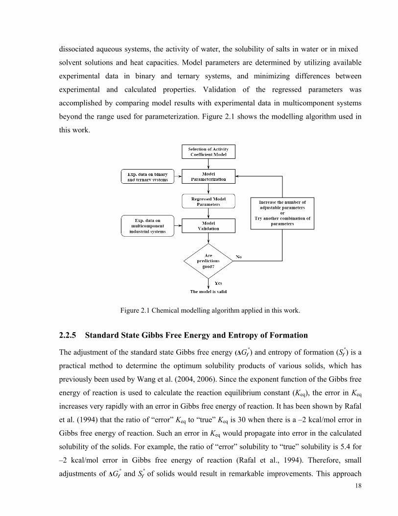
18

dissociated aqueous systems, the activity of water, the solubility of salts in water or in mixed

solvent solutions and heat capacities. Model parameters are determined by utilizing available

experimental data in binary and ternary systems, and minimizing differences between

experimental and calculated properties. Validation of the regressed parameters was

accomplished by comparing model results with experimental data in multicomponent systems

beyond the range used for parameterization. Figure 2.1 shows the modelling algorithm used in

this work.

Figure 2.1 Chemical modelling algorithm applied in this work.

2.2.5 Standard State Gibbs Free Energy and Entropy of Formation

The adjustment of the standard state Gibbs free energy (ΔGfº) and entropy of formation (Sf

º) is a

practical method to determine the optimum solubility products of various solids, which has

previously been used by Wang et al. (2004, 2006). Since the exponent function of the Gibbs free

energy of reaction is used to calculate the reaction equilibrium constant (Keq), the error in Keq

increases very rapidly with an error in Gibbs free energy of reaction. It has been shown by Rafal

et al. (1994) that the ratio of “error” Keq to “true” Keq is 30 when there is a –2 kcal/mol error in

Gibbs free energy of reaction. Such an error in Keq would propagate into error in the calculated

solubility of the solids. For example, the ratio of “error” solubility to “true” solubility is 5.4 for

–2 kcal/mol error in Gibbs free energy of reaction (Rafal et al., 1994). Therefore, small

adjustments of ΔGfº and Sf

º of solids would result in remarkable improvements. This approach

19

gives better extrapolation behavior for the model with respect to temperature, as compared to

fitting empirical parameters in the solubility product equation, the practice which has been used

in previous studies (Li and Demopoulos, 2007, 2006b; Adams, 2004). In the present work, ΔGfº

and Sfº of several solids were adjusted by fitting the experimental solubility data over the entire

temperature range; the regressed values are presented in Appendix B (Table B.2).

2.3 Results and Discussion

Zinc processing solutions typically contain ZnSO4, H2SO4, Fe2(SO4)3, MgSO4, Na2SO4, and

(NH4)2SO4. In order to model the solubility of calcium sulphate hydrates in such solutions, the

solubility of various metal sulphates in water (binary systems) was first verified to determine

whether the default databank (ver. 8.1.3) of the OLI software is capable of reproducing the

available experimental data, or whether it was necessary to perform an estimation of the

parameters through the OLI built-in regression feature. Then, the solubility of CaSO4 in ternary

systems of CaSO4–MSO4–H2O, where M is Zn, Fe(III), Mg, Na, and Mn, and in the system of

CaSO4–H2SO4–H2O was investigated. In most cases, interactions between the various dominant

species are significant and need to be taken into account. Therefore, the MSE interaction

parameters were regressed for better performance of the model. A list of the various systems

studied in this work along with the typical range of conditions investigated is given in Table 2.1.

The obtained model parameters as well as regressed values for the standard state Gibbs free

energy and entropy of the different solids studied are presented in Appendix B.

Table 2.1–Binary and ternary systems studied for the parameterization purpose

System Data type Temperature range, ºC Solid phase

MnSO4-H2O γ± - aw - Cp - solubility 0-180 MnSO4•7H2O, MnSO4•5H2O, MnSO4•1H2O

MgSO4-H2O γ± - aw - solubility 0-250 MgSO4•7H2O, MgSO4•6H2O, MgSO4•1H2O

Na2SO4-H2O γ± - aw - solubility 0-240 Na2SO4•10H2O, Na2SO4

ZnSO4-H2O γ± - aw - solubility 0-300 ZnSO4•7H2O, ZnSO4•6H2O, ZnSO4•1H2O

NiSO4-H2O γ± - solubility 0-300 NiSO4•7H2O, NiSO4•6H2O, NiSO4•1H2O

CaSO4-H2O solubility 0-300 CaSO4•2H2O, CaSO4•0.5H2O, CaSO4 Bin

ary

syst

ems

Fe2(SO4)3-H2O γ± - aw 25 –

20

System Data type Temperature range, ºC Solid phase

CaSO4-(NH4)2SO4-H2O solubility 25-100 CaSO4•2H2O, CaSO4

Al2(SO4)3-H2SO4-H2O solubility 25-60 Al2(SO4)3•16H2O

Fe2(SO4)3-H2SO4-H2O solubility 25-140 Fe2(SO4)3•9H2O, Fe2(SO4)3•6H2O, Fe2(SO4)3

CaSO4-MnSO4-H2O solubility 25-100 CaSO4•2H2O

CaSO4-MgSO4-H2O solubility 25-175 CaSO4•2H2O, CaSO4•0.5H2O, CaSO4

CaSO4-Na2SO4-H2O solubility 25-300 CaSO4•2H2O, CaSO4

NiSO4-H2SO4-H2O solubility 20-300 NiSO4•6H2O, NiSO4•1H2O

MnSO4-H2SO4-H2O solubility 25-65 MnSO4•1H2O

CaSO4-H2SO4-H2O solubility 25-300 CaSO4•2H2O, CaSO4•0.5H2O, CaSO4

CaSO4-ZnSO4-H2O solubility 25-200 CaSO4•2H2O, CaSO4•0.5H2O, CaSO4

CaSO4-NiSO4-H2O solubility 25-175 CaSO4•2H2O, CaSO4

Ter

nary

syst

ems

ZnSO4-H2SO4-H2O solubility 15-70 ZnSO4•7H2O, ZnSO4•6H2O, ZnSO4•1H2O

A list of multicomponent zinc processing systems used for validation purpose is summarized in

Table 2.2. Predicted model results, utilizing the newly regressed parameters obtained in the

binary and ternary systems, are in good agreement with these data, without additional fitting

over the temperature range studied, i.e., 25–90ºC. The Absolute Average Relative Deviations

(AARD%1) between the experimental data and predicted results obtained from the model are

also presented Table 2.2.

Table 2.2–Multicomponent systems studied for validating the model along with AARD% between experimental data and predicted results

System Temperature Range, ºC Solid Phase AARD%

CaSO4-ZnSO4-H2SO4(0.1M)-H2O 25-90 CaSO4•2H2O 5.8 CaSO4-H2SO4-ZnSO4(1.5M)-H2O 25-90 CaSO4•2H2O 5.6 CaSO4-MgSO4-ZnSO4(1.15M)-H2SO4(0.1M)-H2O 25-90 CaSO4•2H2O 5.2 CaSO4-MgSO4-ZnSO4(1.15M)-H2SO4(0.3M)-H2O 25-90 CaSO4•2H2O 8.6 CaSO4-Fe2(SO4)3-ZnSO4(1.15M)-H2SO4(0.3M)-H2O 25-90 CaSO4•2H2O 6.4 CaSO4-Na2SO4-ZnSO4(2.5M)-MgSO4(0.41M)-MnSO4(0.18M)-H2SO4(pH=3.8)-H2O 25-90 CaSO4•2H2O 5.9

CaSO4-H2SO4-ZnSO4(2.5M)-MgSO4(0.41M)-MnSO4(0.18M)-H2O 25-90 CaSO4•2H2O 6.5 CaSO4-(NH4)2SO4-ZnSO4(2.5M)-MgSO4(0.41M)-MnSO4(0.18M)-H2SO4(pH=3.8)-H2O 25-90 CaSO4•2H2O 7.0

1

∑−

=NP

i valueExp

valueCalculatedvalueExp

NPAARD

.

.100(%) , NP: total number of experimental points

21

2.3.1 Binary Systems (Metal Sulphate–H2O)

2.3.1.1 CaSO4–H2O System

The solubility of CaSO4 solid phases (dihydrate, hemihydrate, and anhydrite) has been

extensively measured (dihydrate: (Dutrizac, 2002; Power et al., 1966; Marshall and Slusher,

1966; Marshall et al., 1964; Posnjak, 1938; Hill and Wills, 1938; Hill and Yanick, 1935; Hulett

and Allen, 1902); hemihydrate: (Sborgi and Bianchi, 1940; Partridge and White, 1929);

anhydrite: (Templeton and Rodgers, 1967; Marshall et al., 1964; Bock, 1961; Posnjak, 1938;

Straub, 1932; Partridge and White, 1929)). Most of the measurements are in fairly good

agreement with each other. These experimental solubility data were used to verify the OLI®

default databank.

Although the solubility of CaSO4 dihydrate (gypsum) in H2O at 0–110ºC (Figure 2.2) can be

calculated accurately with the OLI default database (version 8.1.3) using the MSE model, there

is no data for hemihydrate (CaSO4.0.5H2O) in the OLI default database. Therefore, literature

solubility data (Sborgi and Bianchi, 1940; Partridge and White, 1929) were used to adjust the

standard state Gibbs free energy, and entropy of formation of the solid as a function of

temperature, up to 200ºC. The regressed solubility curve is presented in Figure 2.3.

0 20 40 60 80 100 1200.010

0.011

0.012

0.013

0.014

0.015

0.016

0.017

Gyp

sum

Sol

ubili

ty, m

olal

Temperature, oC

OLI default database Exp. data

Figure 2.2 Gypsum solubility in H2O vs. temperature. Experimental data are from Dutrizac, 2002; Power et al., 1966; Marshall and Slusher, 1966; Marshall et al., 1964; Posnjak, 1938; Hill and Wills, 1938; Hill and Yanick, 1935; Hulett and Allen, 1902. The curve is determined from the OLI default database.

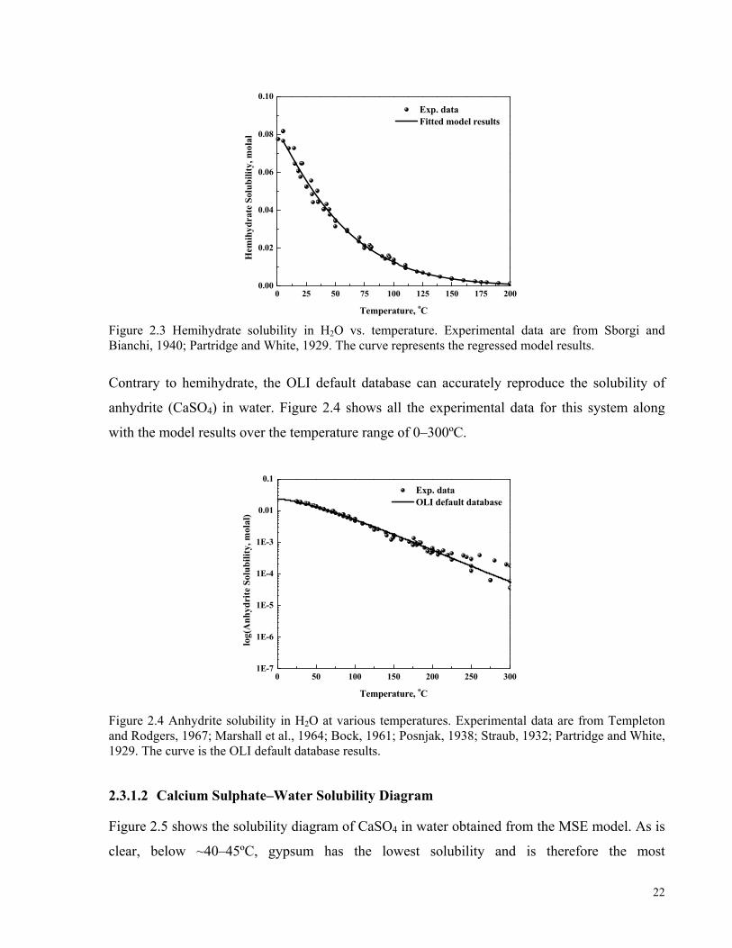
22

0 25 50 75 100 125 150 175 2000.00

0.02

0.04

0.06

0.08

0.10

Hem

ihyd

rate

Sol

ubili

ty, m

olal

Temperature, oC

Exp. data Fitted model results

Figure 2.3 Hemihydrate solubility in H2O vs. temperature. Experimental data are from Sborgi and Bianchi, 1940; Partridge and White, 1929. The curve represents the regressed model results.

Contrary to hemihydrate, the OLI default database can accurately reproduce the solubility of

anhydrite (CaSO4) in water. Figure 2.4 shows all the experimental data for this system along

with the model results over the temperature range of 0–300ºC.

0 50 100 150 200 250 3001E-7

1E-6

1E-5

1E-4

1E-3

0.01

0.1

log(

Anh

ydri

te S

olub

ility

, mol

al)

Temperature, oC

Exp. data OLI default database

Figure 2.4 Anhydrite solubility in H2O at various temperatures. Experimental data are from Templeton and Rodgers, 1967; Marshall et al., 1964; Bock, 1961; Posnjak, 1938; Straub, 1932; Partridge and White, 1929. The curve is the OLI default database results.

2.3.1.2 Calcium Sulphate–Water Solubility Diagram

Figure 2.5 shows the solubility diagram of CaSO4 in water obtained from the MSE model. As is

clear, below ~40–45ºC, gypsum has the lowest solubility and is therefore the most

23

thermodynamically stable phase. The transition point of gypsum to anhydrite lies at 40±5ºC,

and that of gypsum to hemihydrate lies at 99±5ºC.

0 50 100 150 200 250 3000.00

0.01

0.02

0.03

0.04

0.05

0.06

0.07

0.08

gypsum

anhydrite

Cal

cium

Sul

phat

e So

lubi

lity,

mol

al

Temperature, oC

hemihydrate

Figure 2.5 Solubility diagram of CaSO4 in H2O. The solid and dashed curves show the stable and metastable phases, respectively, at a given temperature.

In the region between these two temperatures, gypsum is metastable, although the degree of

metastability in dilute aqueous solutions is significant. Thus, gypsum–water slurries can be

heated to 100ºC without transforming gypsum to anhydrite or hemihydrate. In contrast, gypsum

transforms rapidly to anhydrite in concentrated acid–salt solutions at temperatures above 70–

80ºC (Dutrizac, 2002). More details regarding the gypsum transformation in such systems are

available in Chapter 5.

2.3.1.3 MnSO4–H2O System

There are no relevant data for MnSO4 in the OLI default database. Therefore, experimental data

on the solubility of MnSO4 in H2O (Linke and Seidell, 1958), the mean activity coefficient (γ±)

(Guendouzi et al., 2003), the activity of water (awater) (Guendouzi et al., 2003) and heat capacity

(Cp) (Aseyev, 1996) were used to regress model parameters including the standard state Gibbs

free energy and entropy of formation of the solids; i.e., MnSO4•7H2O, MnSO4•5H2O, and

MnSO4•1H2O as a function of temperature. In addition, MSE middle-range interaction

parameters between Mn2+ and SO42- ions were regressed. The solubility curve of this system is

shown in Figure 2.6.

24

0 30 60 90 120 150 1800.0

0.5

1.0

1.5

2.0

2.5

3.0

3.5

4.0

4.5

5.0

MnSO4.7H

2O

MnSO4.5H

2O

MnS

O4 so

lubi

lity,

mol

al

Temperature, oC

MnSO4.7H

2O Exp. Data

MnSO4.5H2O Exp. Data MnSO

4.1H

2O Exp. Data

MnSO4.1H2O

Figure 2.6 Solubility of MnSO4 in H2O. Experimental data are from Linke and Seidell (1958); curve shows the model results.

2.3.1.4 NiSO4–H2O System

Experimental data on the mean activity coefficient, the activity of water, and the solubility of

NiSO4 (Linke and Seidell, 1958; Robinson and Stokes, 2002; Bruhn et al., 1965) were used to

fit the MSE middle-range interaction parameters between Ni2+ and SO42- ions, as well as the

standard state Gibbs free energy and entropy of the solids, NiSO4•7H2O, NiSO4•6H2O, and

NiSO4•1H2O, as a function of temperature. Figure 2.7 shows the solubility of NiSO4 in H2O up

to 300°C.

0 50 100 150 200 250 3000.0

0.5

1.0

1.5

2.0

2.5

3.0

3.5

4.0

4.5

5.0

5.5

6.0

NiSO4.1H2O

NiSO4.6H2O

NiS

O4 so

lubi

lity,

mol

al

Temperature, oC

NiSO4.7H2O Exp data NiSO4.6H2O Exp data NiSO4.1H2O Exp data

NiSO4.7H2O

Figure 2.7 Solubility of NiSO4 in H2O at various temperatures. Experimental data are from Linke and Seidell (1958) and Bruhn et al. (1965); curve shows the fitted model results.

25

No additional fitting was carried out on the MgSO4, ZnSO4 and Na2SO4 aqueous metal

sulphate systems, because the OLI default database (ver. 8.1.3) was found to predict these

systems accurately.

2.3.1.5 Fe2(SO4)3–H2O System

No reliable data are available on the solubility of Fe2(SO4)3 in water, the mean activity

coefficient of Fe2(SO4)3 solutions and the activity of water. The solubility in this system is

difficult to study mainly because of the pronounced tendency of Fe2(SO4)3 to hydrolyse in

aqueous solutions and form a variety of precipitates. The solutions formed are a yellow-brown

colour, as a result of the presence of Fe(III)–hydroxyl ions (hydrated Fe3+ ions are nearly

colourless) (Kononova and Redzhepov, 1996).

2.3.2 Ternary (Metal sulphate–H2SO4–H2O) Systems

2.3.2.1 CaSO4–H2SO4–H2O System

The solubility of CaSO4 hydrates in H2SO4 solutions has been measured by Ling and

Demopoulos (2004), Dutrizac (2002), Zdanovskii and Vlasov (1968), Zdanovskii et al. (1968)

and Marshall and Jones (1966). The OLI default database does not predict the solubility

behaviour in this system accurately. Consequently, experimental data for gypsum, hemihydrate

and anhydrite were used to regress the MSE middle range interaction parameters between the

Ca2+–HSO4¯ and CaSO4(aq)–HSO4

¯ species over the temperature of 25–300ºC. Figure 2.8 shows

the experimental data along with the fitted model results for gypsum at 25–95ºC and that of

anhydrite at 150–250ºC. As can be seen, the model fits the experimental data accurately for both

solids over the whole temperature range (AARD%=6.0). Figure 2.9 shows the three–

dimensional solubility diagram of this system.

At low temperatures (25–60°C), the addition of H2SO4 increases the solubility of gypsum

moderately, whereas at higher temperatures, the solubility increases strongly with increasing

acid concentration. This behaviour is due to the decrease of the second dissociation constant of

H2SO4 with increasing temperature. Thus, the addition of H2SO4 to saturated CaSO4–H2O

solutions reduces the SO42- concentration and allows an increase in the solubility of CaSO4 to

satisfy the solubility product (Marshall and Jones, 1966).

26

0.0 0.5 1.0 1.5 2.0 2.5 3.00.00

0.02

0.04

0.06

0.08

0.10

0.12Solid phase: CaSO4

Exp data, 150 oC Exp data, 200 oC Exp data, 250 oC

Solid phase: CaSO4.2H2O

Exp data, 25 oC Exp data, 50 oC Exp data, 75 oC Exp data, 90 oC

CaS

O4 so

lubi

lity,

mol

al

H2SO4, molal

Figure 2.8 CaSO4 solubility in ternary system of CaSO4–H2SO4–H2O. Curves show the regressed model results. Experimental data are from (Dutrizac, 2002; Zdanovskii et al., 1968; Marshall and Jones, 1966).

01

23

4 3040

5060

7080

900.02

0.04

0.06

0.08

0.10

0.12

gypsum

anhydrite

CaS

O4 so

lubi

lity,

mol

al

Tempera

ture, o CH

2 SO4 , molal

hemihydrate

Figure 2.9 Solubility diagram of CaSO4 in H2SO4–H2O solutions; the surfaces were obtained from the model.

Moreover, as the H2SO4 concentration increases from pure water, the solubility of gypsum

increases gradually. After passing a maximum, the solubility decreases smoothly with further

increasing acid concentration. The initial increase is due to the formation of bisulphate ions. The

solubility decrease in concentrated H2SO4 solutions can be explained by the concept of

solvation: as the concentration of electrolyte increases, fewer water molecules can participate in

the dissolution process because they are tightly held (solvated) by cations and anions in the

solution, this is known as the salting-out effect (Görgényi et al., 2006; Kessler et al., 1963).

27

The phase transition between gypsum–anhydrite and gypsum–hemihydrate was determined on

the basis of phase solubilities. At the transition point, where there is equilibrium between two

phases, the solubilities of both phases are equal. Figure 2.10 shows the phase transition

diagrams of gypsum–anhydrite and gypsum–hemihydrate in H2SO4–H2O solutions obtained on

the basis of solubility curves calculated from the new model.

0 1 2 3 4 5 6 70

102030405060708090

100110120130140

Anhydrite stable

IIIHemihydrate metastable

IIGypsum metastable

Tem

pera

ture

, o C

H2SO4, molal

Zdanovskii et al., 1968 Zdanovskii et al., 1968, Ling and Demopoulos, 2004

IGypsum stable

Figure 2.10 Transition diagram of CaSO4 hydrates in CaSO4–H2SO4–H2O system. Region I: gypsum stable, Region II: anhydrite stable, gypsum metastable, Region III: anhydrite stable, hemihydrate metastable. Experimental data are from Zdanovskii et al. (1968), Ling and Demopoulos (2004).

To validate the diagram, available experimental data, measured by Zdanovskii et al. (1968) up

to 95°C and by Ling and Demopoulos (2004) at 100°C, are also presented on the graph. The

phase diagram was constructed using a procedure similar to the one suggested by Li and

Demopoulos (2006c). Based on the diagram, the gypsum–anhydrite and gypsum–hemihydrate

transformation in water takes place at around 40ºC and 100ºC, respectively. However, the

kinetics of these transformations is slow, resulting in gypsum retention as a metastable phase for

longer periods of time. Transformation kinetics was investigated more thoroughly and more

details are available in Chapter 5.

2.3.2.2 NiSO4–H2SO4–H2O System

The solubility of NiSO4 in aqueous sulphuric acid solutions was studied by Kudryashov and

Lebedev (1989), Girich and Buchinskii (1986) and Marshall et al. (1962). Additional fittings

were performed for the Ni2+–HSO4¯ MSE middle range parameters to improve the prediction of

the chemistry for the system. The results obtained from the fitting compared with the

28

experimental data over a temperature range of 20–300ºC are shown in Figures 2.11 and 2.12.

As is clear, the model results are in good agreement with the experimental data (AARD%=9 for

80 points).

0.0 0.5 1.0 1.5 2.0 2.5 3.0 3.5 4.0 4.50

1

2

3

4

5

6

7

8

60 oC

40 oC

Solid phase: NiSO4.6H2O

Exp data, 20 oC Exp data, 40 oC Exp data, 60 oC

NiS

O4 so

lubi

lity,

mol

al

H2SO

4, molal

20 oC

Figure 2.11 NiSO4 solubility in aqueous H2SO4 solutions below 100ºC; experimental data are from Kudryashov (1989), and Girich (1986). The curves are the regressed model results.

0.0 0.2 0.4 0.6 0.8 1.0 1.2 1.4 1.60.0

0.5

1.0

1.5

2.0

2.5

3.0

250 oC

300 oC275 oC

200 oC

Solid phase: NiSO4.1H2O

Exp data, 200 oC Exp data, 250 oC Exp data, 275 oC Exp data, 300 oC

NiS

O4 so

lubi

lity,

mol

al

H2SO

4, molal

Figure 2.12 NiSO4 solubility in aqueous H2SO4 solutions above 200ºC; experimental data are from Marshall et al. (1962). The curves are the regressed model results.

2.3.2.3 MnSO4–H2SO4–H2O System

The experimental data for this system were selected from the Linke and Seidell (1958) solubility

data collection. Regression was performed on the model parameters between the Mn2+–HSO4¯

and MnSO4(aq)–HSO4¯ species to obtain an acceptable model prediction. The fitted results

29

corresponding to the experimental data are shown in Figure 2.13, which are in good agreement

(AARD%=5.8).

0.0 0.5 1.0 1.5 2.0 2.5 3.0 3.50.0

0.5

1.0

1.5

2.0

2.5

3.0

3.5

4.0

4.5

5.0

65 oC

45 oC

MnS

O4 so

lubi

lity,

mol

al

H2SO4, molal

Solid phase: MnSO4.1H2O

Exp data, 25 oC Exp data, 45 oC Exp data, 65 oC

25 oC

Figure 2.13 MnSO4 solubility in aqueous H2SO4 solutions; experimental data are from Linke and Seidell (1958), and the curves are the regressed model results.

2.3.2.4 Al2(SO4)3–H2SO4–H2O System

The experimental data for this system were reported by Linke and Seidell (1958). The default

MSE database (ver. 8.1.3) of the OLI does not predict the solubility behaviour of this system

accurately. Consequently, regression was performed on the MSE middle-range interaction

parameters between the Al(SO4)2¯–H3O+ and AlSO4

+–HSO4¯ species to allow an acceptable

model prediction (presented in Appendix B). The fitted results along with the experimental data

are shown in Figure 2.14; the results accurately reflect the experimental data (AARD%=2.4).

0.0 0.5 1.0 1.5 2.00.0

0.2

0.4

0.6

0.8

1.0

1.2

1.4

1.6

1.8

2.0

60 oC

50 oC

Al 2(S

O4) 3 so

lubi

lity,

mol

al

H2SO

4, molal

Solid phase: Al2(SO

4)

3.16H

2O

Exp data, 25 oC Exp data, 50 oC Exp data, 60 oC

25 oC

Figure 2.14 Aluminum sulphate solubility in H2SO4 solutions; experimental data are from Linke and Seidell (1958) and the curves are the fitted model.

30

No additional fitting was carried out on the MgSO4, ZnSO4, Na2SO4, and Fe2(SO4)3 in H2SO4

aqueous systems, because the OLI default database (ver.8.1.3) was found to predict these

systems accurately.

2.3.3 Ternary (CaSO4–Metal sulphate–H2O) Systems

2.3.3.1 CaSO4–ZnSO4–H2O System

The solubility of calcium sulphate in the CaSO4–ZnSO4–H2O system was studied by Umetsu et

al. (1989) and Zatonskaya et al. (1988) over the temperature range of 25–150ºC. Their

experimental solubility data were used to regress the MSE middle range interaction parameters

between Zn2+ and Ca2+ as well as Zn2+ and CaSO4(aq). In this system, Ca2+ is the dominant

calcium species at lower concentrations of ZnSO4, whereas at higher concentrations, the neutral

calcium sulphate ion pair (CaSO4(aq)) becomes dominant. Figures 2.15 and 2.16 show the model

results compared with the experimental data.

As is clear, the model accurately reflects the experimental data (AARD%=5.5). Also, it is clear

that calcium sulphate dihydrate is the stable solid phase up to 90ºC and calcium sulphate

hemihydrate is the stable phase from 100°C to 150ºC. These results are consistent with the XRD

data reported by Umetsu et al. (1989).

0.0 0.4 0.8 1.2 1.6 2.0 2.40.00

0.01

0.02

0.03

0.04

0.05

0.06

90 oC70 oC

40 oC

CaS

O4 so

lubi

lity,

mol

al

ZnSO4, molal

Solid phase: CaSO4.2H2O

Exp data, 25 oC Exp data, 40 oC Exp data, 70 oC Exp data, 90 oC

25 oC

Figure 2.15 CaSO4 solubility in ZnSO4 solutions below 100ºC; experimental data are from Umetsu et al. (1989) and Zatonskaya et al. (1988), and the curves are fitted model results.

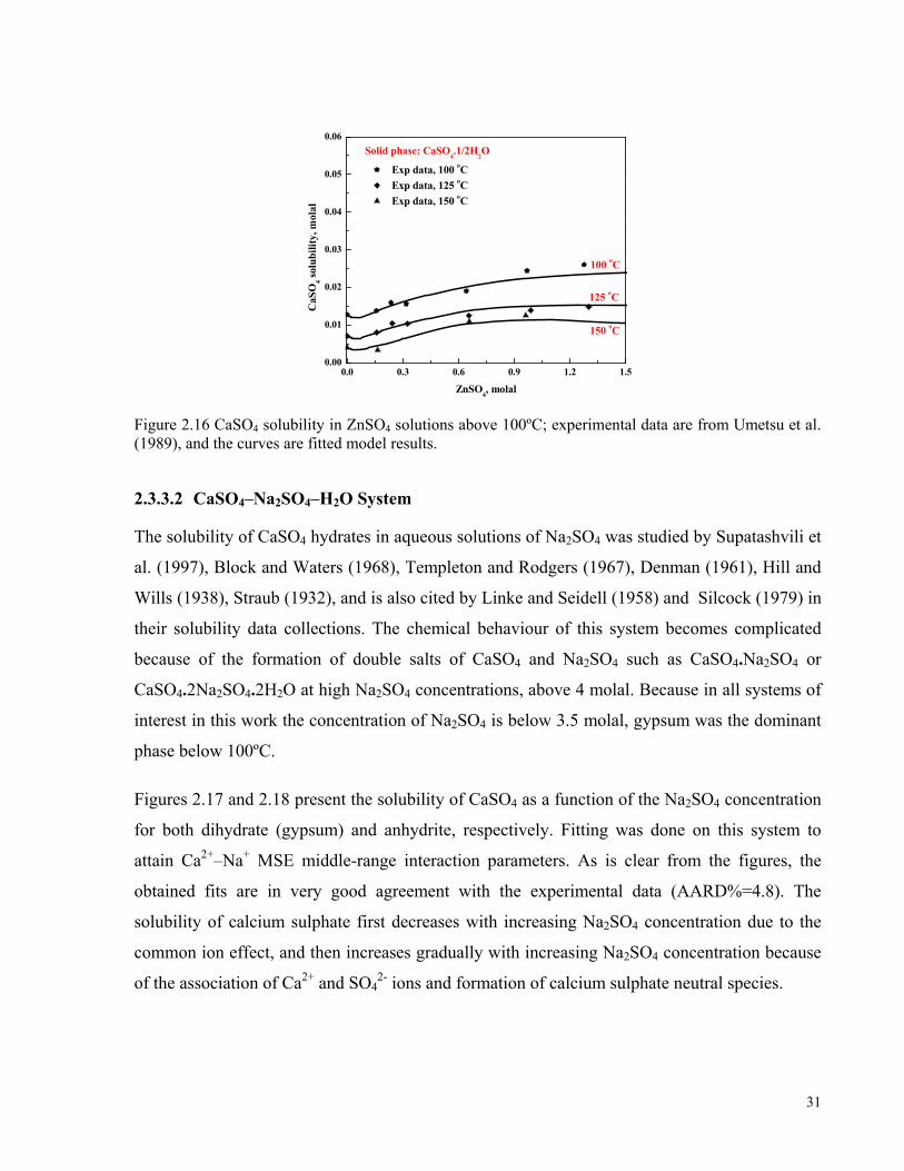
31

0.0 0.3 0.6 0.9 1.2 1.50.00

0.01

0.02

0.03

0.04

0.05

0.06

150 oC

125 oC

Solid phase: CaSO4.1/2H

2O

Exp data, 100 oC Exp data, 125 oC Exp data, 150 oC

CaS

O4 so

lubi

lity,

mol

al

ZnSO4, molal

100 oC

Figure 2.16 CaSO4 solubility in ZnSO4 solutions above 100ºC; experimental data are from Umetsu et al. (1989), and the curves are fitted model results.

2.3.3.2 CaSO4–Na2SO4–H2O System

The solubility of CaSO4 hydrates in aqueous solutions of Na2SO4 was studied by Supatashvili et

al. (1997), Block and Waters (1968), Templeton and Rodgers (1967), Denman (1961), Hill and

Wills (1938), Straub (1932), and is also cited by Linke and Seidell (1958) and Silcock (1979) in

their solubility data collections. The chemical behaviour of this system becomes complicated

because of the formation of double salts of CaSO4 and Na2SO4 such as CaSO4.Na2SO4 or

CaSO4.2Na2SO4.2H2O at high Na2SO4 concentrations, above 4 molal. Because in all systems of

interest in this work the concentration of Na2SO4 is below 3.5 molal, gypsum was the dominant

phase below 100ºC.

Figures 2.17 and 2.18 present the solubility of CaSO4 as a function of the Na2SO4 concentration

for both dihydrate (gypsum) and anhydrite, respectively. Fitting was done on this system to

attain Ca2+–Na+ MSE middle-range interaction parameters. As is clear from the figures, the

obtained fits are in very good agreement with the experimental data (AARD%=4.8). The

solubility of calcium sulphate first decreases with increasing Na2SO4 concentration due to the

common ion effect, and then increases gradually with increasing Na2SO4 concentration because

of the association of Ca2+ and SO42- ions and formation of calcium sulphate neutral species.

32

0.0 0.5 1.0 1.5 2.0 2.5 3.0 3.50.00

0.01

0.02

0.03

0.04

0.05

75 oC

50 oC

CaS

O4 so

lubi

lity,

mol

al

Na2SO4, m

Solid phase: CaSO4.2H2O

Exp data, 25 oC Exp. data, 50 oC Exp. data, 75 oC

25 oC

Figure 2.17 CaSO4 solubility in Na2SO4 solutions below 100ºC; experimental data are from Block and Waters (1968), Denman (1961), Hill and Wills (1938). The curves are the fitted model.

0.0 0.5 1.0 1.5 2.0 2.5 3.0 3.5 4.00.000

0.005

0.010

0.015

0.020

0.025

0.030

0.035

0.040

100 oC

75 oC

CaS

O4 so

lubi

lity,

mol

al

Na2SO

4, m

Solid phase: CaSO4

Exp. data, 50 oC Exp. data, 75 oC Exp. data, 100 oC Exp. data, 207 oC Exp. data, 300 oC

50 oC

Figure 2.18 CaSO4 solubility in Na2SO4 solutions above 100ºC; experimental data are from Block and Waters (1968), Templeton and Rodgers (1967), Hill and Wills (1938), Straub (1932). The curves are the fitted model.

2.3.3.3 CaSO4–NiSO4–H2O System

The solubility of CaSO4 dihydrate in aqueous solutions of NiSO4 has been measured by

Campbell and Yanick (1932) from 45°C to 95ºC and also by Wollmann and Voigt (2008) at

25ºC and 45ºC. The lowest NiSO4 concentration examined by Campbell and Yanick (1932) was

0.4 molal, and therefore, they missed the minimum solubility of gypsum due to the common ion

effect. The solubility data measured by Wollmann and Voigt (2008) at 45ºC agreed with

0.00 0.05 0.10 0.15 0.20 0.25 0.30 0.3500

05

0

5

20

25

30

35

40

45

50

300 oC

207 oC

33

Campbell’s results up to 1.5 molal NiSO4, however, at higher concentrations, the solubility

data measured by Wollmann and Voigt (2008) were lower than those measured by Campbell

and Yanick (1932). This is due to the method of calcium analysis used by Campbell and Yanick

(1932). In their work, calcium was analyzed gravimetrically as calcium oxalate monohydrate.

Because nickel oxalate dihydrate, Ni(C2O4)•2H2O(s), has a similar solubility as calcium oxalate,

it creates a bias towards higher apparent calcium sulfate concentrations.

To obtain reliable data, the solubility of gypsum in aqueous NiSO4 systems was measured at 25–

95ºC in this work. Also, anhydrite solubility was measured inside an autoclave at elevated

temperatures of 150°C and 175ºC. The experimental procedure is discussed in detail in Chapter

4. Tables C.1 and C.2 in Appendix C summarize the newly measured data for gypsum and

anhydrite in this system. These data were combined with those measured by Campbell and

Yanick (1932) (below 1.5 molal NiSO4) and those of Wollmann and Voigt (2008) and were

used to regress the MSE middle range interaction parameters between calcium species, Ca2+ and

CaSO4(aq), and Ni2+ ions. The regressed model results are shown in Figures 2.19 and 2.20. As

can be seen, the model fits the experimental data accurately with an absolute average relative

deviation (AARD%) of 5.6 for 116 points.

0.0 0.5 1.0 1.5 2.0 2.5 3.0 3.50.000

0.005

0.010

0.015

0.020

0.025

0.030

0.035

0.040

0.045

90 oC

45 oC

Solid: CaSO4.2H2O

This work+Wollmann (2008) Exp data, 25oC This work+Campbell (1932) Exp data, 45oC This work+Campbell (1932) Exp data, 90oC

CaS

O4 so

lubi

lity,

mol

al

NiSO4, molal

25 oC

Figure 2.19 Gypsum solubility in NiSO4 solutions below 100ºC. Experimental data are from Azimi and Papangelakis (2010b), Wollmann and Voigt (2008) and Campbell and Yanick (1932); the curves are the fitted model.

34

0.0 0.2 0.4 0.6 0.80.000

0.002

0.004

0.006

0.008

150 oC

175 oC

Solid phase: CaSO4

This work, 150 oC This work, 175 oC

CaS

O4 so

lubi

lity,

mol

al

NiSO4, molal

Figure 2.20 Anhydrite solubility in NiSO4 solutions above 100ºC. Experimental data are from Azimi and Papangelakis (2010b); the curves are the fitted model.

As the NiSO4 concentration increases from pure water, the solubility of gypsum initially drops

and then increases gradually with increasing NiSO4 concentration. After passing a maximum,

the solubility decreases smoothly with further increasing NiSO4 concentration. The initial drop

is due to the common ion effect, shifting the dissolution reaction (equation 2.1) to the left; the

subsequent increase is attributable to the association of Ca2+ and SO42- ions and formation of

calcium sulphate neutral species (equation 2.2). The solubility decrease in concentrated NiSO4

solutions can be explained by the salting-out effect, which is a result of reduced number of free

water molecules in the solution to dissolve calcium sulphate.

According to equations (2.7) and (2.8), the solubility of calcium sulphate is equal to the sum of

+2Cam and

)(4 aqCaSOm which are inversely proportional to )( 2)( 4

24

nwCaSOSO

am ⋅⋅ ±− γ and )()(4

nwCaSO a

aq⋅γ ,

respectively. Figure 2.21 presents the solubility of gypsum (dihydrate) along with +2Cam and

)(4 aqCaSOm as well as )( 22)( 4

24

wCaSOSO am ⋅⋅ ±− γ and )( 2)(4 wCaSO a

aq⋅γ terms calculated by the aid of the MSE

model containing regressed interaction parameters as a function of the NiSO4 concentration at

90ºC. As is clear, the value of )( 2)(4 wCaSO a

aq⋅γ term decreases with an increase in NiSO4

concentration, reaching a minimum at ~2 molal which corresponds to the maximum of the

solubility curve. Above this point, the value of )( 2)(4 wCaSO a

aq⋅γ term increases gradually as a result

35

of the increase in )(4 aqCaSOγ with concentration due to the salting-out effect, resulting in a decrease

in the concentration of CaSO4(aq) and consequently, the decrease in gypsum solubility.

0.0 0.5 1.0 1.5 2.0 2.5 3.0 3.50.00

0.01

0.02

0.03

0.04

0.05

0.06

mSO4

2- * aw2 * γ±

2

Solid phase: CaSO4.2H2O

Con

cent

ratio

n, m

olal

NiSO4, molal

γCaSO4(a)

* aw2 * 10-1

T= 90 oC

solubility curve

[Ca2+]

[CaSO4(aq)

]

[Catotal

]

Figure 2.21 Total concentration of Ca along with Ca2+ and CaSO4(aq) concentrations in CaSO4–NiSO4–H2O system at 90ºC. Calculated values of ( 22

)( 424

wCaSOSOam ⋅⋅ ±− γ ) and ( 2

)(4 wCaSO aaq⋅γ ) are also presented.

2.3.3.4 CaSO4–MgSO4–H2O System

The solubility of gypsum in aqueous MgSO4 solutions at different temperatures was measured

by different researchers (Wollmann and Voigt, 2008; Arslan and Dutt, 1993; Umetsu et al.,

1989; Tanji, 1969; Novikova, 1957) and was also cited by Linke and Seidell (1958) in their

solubility data compilation. Umetsu et al. (1989) also measured the solubility of calcium

sulphate at elevated temperatures at 100–175ºC. They observed that the solid phases

corresponding to their solubility data were hemihydrate between 100°C and 150ºC and

anhydrite above 150ºC. These data were used to regress the MSE middle range interaction

parameters between Ca2+–Mg2+ as well as CaSO4(aq)–Mg2+ species. The modelling results

showed that the experimental data measured by Umetsu et al. (1989) above 150ºC, closely

match the solubility of hemihydrate instead of that of anhydrite. Therefore, in this work, the

solubility of anhydrite was measured in an autoclave at 150°C and 175ºC in aqueous MgSO4

solutions which are summarized in Appendix C (Table C.3). Details regarding the experimental

procedure are available in Chapter 4. The newly measured data were compiled along with other

experimental data in a data regression file to regress the interaction parameters between Mg2+

and the calcium species. Figures 2.22 to 2.24 show the model results in comparison with the

experimental data for gypsum, hemihydrate and anhydride, respectively.

36

0.0 0.5 1.0 1.5 2.0 2.5 3.00.00

0.01

0.02

0.03

0.04

0.05

0.06

75 oC

45 oC

CaS

O4 so

lubi

lity,

mol

al

MgSO4, molal

Solid phase: CaSO4.2H2O

Exp data, 25 oC Exp data, 45 oC Exp data, 75 oC

25 oC

Figure 2.22 Gypsum solubility in aqueous MgSO4 solutions. Experimental data are from Tanji (1969), Arslan and Dutt (1993), Umetsu et al. (1989), Linke and Seidell (1958); the curves are the fitted model.

0.0 0.1 0.2 0.3 0.4 0.5 0.6 0.7 0.8 0.90.000

0.005

0.010

0.015

0.020

0.025

0.030

0.035

0.040

100 oC

125 oC

CaS

O4 so

lubi

lity,

mol

al

MgSO4, molal

Solid phase: CaSO4. 1/2 H2O

Exp data, 100 oC Exp data, 125 oC Exp data, 175 oC

175 oC

Figure 2.23 Hemihydrate solubility in aqueous MgSO4 solutions. Experimental data are from Umetsu et al. (1989); the curves are the fitted model.

37

0.0 0.1 0.2 0.3 0.4 0.5 0.6 0.70.000

0.001

0.002

0.003

0.004

0.005

0.006

0.007

175 oC

Solid phase: CaSO4

This work, 150 oC This work, 175 oC

CaS

O4 so

lubi

lity,

mol

al

MgSO4, molal

150 oC

Figure 2.24 Anhydrite solubility in aqueous MgSO4 solutions. Experimental data are from Azimi and Papangelakis (2010b); the curves are the fitted model.

As in the case with NiSO4, the solubility of gypsum first decreases with increasing MgSO4

concentration due to the common ion effect of added SO42- ions and then increases gradually

with increasing MgSO4 concentration because of the association of Ca2+ and SO42- ions and

formation of calcium sulphate neutral species. For concentrated solutions containing more than

1.0–1.5 molal MgSO4, the salting-out effect becomes dominant, and as a result, the solubility

drops accordingly.

2.3.3.5 CaSO4–MnSO4–H2O System

Zhelnin et al. (1973) measured the solubility of CaSO4 in the CaSO4–MnSO4–H2O system from

25°C to 100ºC, and their observations show that in this temperature range, even up to 3.5 molal

MnSO4, gypsum is the only solid in equilibrium with the solution. Wollmann and Voigt (2008)

also measured CaSO4 solubility in this system at 25ºC and 40ºC. All the experimental data were

used to fit Ca2+–Mn2+ and also CaSO4(aq)–Mn2+ MSE interaction parameters, because at higher

concentrations of MnSO4, CaSO4(aq) is more abundant than the Ca2+ species. The fitted results

for this system are shown in Figure 2.25, and the calculated solubilities are consistent with the

experimental data (AARD%=5.9).

38

0.0 0.5 1.0 1.5 2.0 2.5 3.0 3.50.00

0.01

0.02

0.03

0.04

0.05

0.06

100 oC

50 oC

75 oC

CaS

O4 so

lubi

lity,

mol

al

MnSO4, molal

Solid phase: CaSO4.2H

2O

Exp data, 25 oC Exp data, 50 oC Exp data, 75 oC Exp data, 100 oC

25 oC

Figure 2.25 CaSO4 solubility in MnSO4 solutions; experimental data are from Wollmann and Voigt (2008) and Zhelnin et al. (1973), and the curves are the fitted model.

2.3.4 Effect of Divalent Cations on the Solubility of CaSO4

Figure 2.26 presents a comparison between the solubility of CaSO4 dihydrate (gypsum) in

ternary solutions of CaSO4–NiSO4–H2O, CaSO4–MgSO4–H2O and CaSO4–MnSO4–H2O along

with the model predictions at two different temperatures of 25ºC and 75°C. It is clear that the

difference between CaSO4 solubilities in these systems at both temperatures is always less than

15% indicating that the cation type does not have a dramatic effect on the CaSO4 solubility. For

all three cations, as the metal sulphate concentration increases from pure water, the solubility

initially drops and then increases gradually. After passing a maximum, the solubility decreases

smoothly with further increasing the MSO4 (M=Mg, Mn, Ni) concentration. The initial drop is

due to the common ion effect which shifts the dissolution reaction (Eq. 2.1) to the left; the

subsequent increase is attributable to the association of Ca2+ and SO42- ions and formation of

calcium sulfate neutral species (Eq. 2.2). The solubility decrease in concentrated solutions is due

to the salting-out effect. Moreover, for all three cations, gypsum solubility increases with

increasing temperature due to the fact that the association constant (Ka) of CaSO4(aq) increases

with temperature, which would shift Eq. 2.2 to the right.

In industrial applications, particularly in hydrometallurgy, solutions usually contain several

cations for which there are no experimental data available. By knowing that cation type does not

have a significant effect on the solubility behaviour, all divalent cations can be substituted with

a certain cation for which experimental data are available during the simulation of the process.

39

0.00 0.25 0.50 0.75 1.00 1.25 1.50 1.75 2.000.00

0.01

0.02

0.03

0.04

0.05 MgSO4 solubility MnSO

4 solubility

NiSO4 solubility

T=25 oC

CaS

O4 so

lubi

lity,

mol

al

MSO4 (M=Ni, Mg, Mn), molal

Solid phase: CaSO4.2H2OExp. data:

MgSO4, 25oC

MnSO4, 25oC

NiSO4, 25oC

MgSO4, 75oC

MnSO4, 75oC

NiSO4, 75oC

T=75 oC

Figure 2.26 CaSO4 solubility in MSO4 (M=Ni, Mg, Mn) solutions. Experimental data are from Azimi, Papangelakis (2010b); Wollmann, Voigt (2008); Arslan, Dutt (1993); Zhelnin et al. (1973); Tanji (1969); Campbell,Yanick (1932). Curves represent the model predictions.

2.3.5 Industrial Implications of the Model in Zinc Producing Industries

So far, it has been shown that the MSE model is effective for fitting the solubility of CaSO4

hydrates in binary or ternary electrolyte solutions. In order to validate the model parameters, the

solubility of CaSO4 hydrates was calculated in multicomponent zinc sulphate processing

solutions containing ZnSO4, H2SO4, Fe2(SO4)3, MgSO4, and (NH4)2SO4, for which no fitting

was carried out. As will be seen later in this section, the model is capable of predicting the

chemistry of all the multicomponent systems studied. This fact illustrates the usefulness of the

model, utilizing the developed database, in assessing the scaling potential of calcium sulphate in

a variety of complex aqueous processing streams where no experimental data are available.

2.3.5.1 CaSO4–ZnSO4–H2SO4 (0.1 M)–H2O System

Dutrizac (2002) has studied the effect of ZnSO4 concentration on the solubility of calcium

sulphate in solutions containing 0.1 M H2SO4 as a function of temperature. The solubility of

calcium sulphate decreases steadily as the ZnSO4 concentration increases from 0.0 to 0.5 M

ZnSO4 because of the common ion effect. The experimental data were obtained on heating to

95ºC and on subsequent cooling. In this system, because the acid concentration used is relatively

low, the dehydration of gypsum to anhydrite does not practically occur at temperatures below

95ºC. Figure 2.27 shows the experimental solubility data of CaSO4 vs. ZnSO4 concentration in

40

0.1 M H2SO4 media at various temperatures along with the model predictions. The predictions

are in good agreement with the experimental data (AARD%=5.8).

0.0 0.5 1.0 1.5 2.00.00

0.01

0.02

0.03

0.04

0.05

0.06

90 oC

70 oC

40 oC

CaS

O4 so

lubi

lity,

mol

al

ZnSO4, molal

Solid phase: CaSO4.2H2O

Exp data, 25 oC Exp data, 40 oC Exp data, 70 oC Exp data, 90 oC

25 oC

H2SO4=0.1 M

Figure 2.27 CaSO4 solubility in CaSO4–ZnSO4–H2SO4 (0.1 M)–H2O solutions. Experimental data are from Dutrizac (2002); the curves are the predicted results.

2.3.5.2 CaSO4–H2SO4–ZnSO4 (1.5 M)–H2O System

The solubility of CaSO4 as a function of acid concentration in solutions containing 1.5 M ZnSO4

was also measured by Dutrizac (2002). Figure 2.28 shows the experimental data and the

predicted results from the model. The model predictions are in close agreement with the

experimental data (AARD%=5.6). It is also clear that acid concentration has a relatively minor

effect on the solubility of CaSO4 when the solution contains 1.5 M of ZnSO4. This effect is due

to the free sulphate ions released from the dissociation of ZnSO4.

0.0 0.5 1.0 1.5 2.0 2.50.00

0.01

0.02

0.03

0.04

0.05

0.06

0.07

90 oC

70 oC

40 oC

CaS

O4 so

lubi

lity,

mol

al

H2SO4, molal

Solid phase: CaSO4.2H2O

Exp data, 25 oC Exp data, 40 oC Exp data, 70 oC Exp data, 90 oC

25 oC

ZnSO4=1.5 M

Figure 2.28 CaSO4 solubility in CaSO4–H2SO4–ZnSO4 (1.5M)–H2O solutions. Experimental data are from Dutrizac (2002); the curves are the predicted results.

41

2.3.5.3 CaSO4–MgSO4–H2SO4 (0.1 M)–ZnSO4 (1.15 M)–H2O System

Zinc processing solutions typically contain modest concentrations of MgSO4 and MnSO4

(Dutrizac, 2002). The effect of MgSO4 on the solubility of CaSO4 was studied because its

impact on CaSO4 chemistry was unknown. For this purpose, the solubility of CaSO4 in a system

containing MgSO4, ZnSO4 and H2SO4 was modelled using the new database. As shown in

Figure 2.29, the model is capable of accurately predicting the experimental data in this system

(AARD%=5.2).

0.0 0.2 0.4 0.6 0.8 1.0 1.20.00

0.01

0.02

0.03

0.04

0.05

0.06

ZnSO4=1.5MH2SO4=0.1M

25 oC

40 oC70 oC

CaS

O4 so

lubi

lity,

mol

al

MgSO4, molal

Solid phase: CaSO4.2H

2O

Exp data, 25 oC Exp data, 40 oC Exp data, 70 oC Exp data, 90 oC

90 oC

Figure 2.29 CaSO4 solubility in CaSO4–MgSO4–ZnSO4 (1.15 M)–H2SO4 (0.1 M)–H2O solutions; experimental data are from Dutrizac (2002); curves represent model predictions.

2.3.5.4 CaSO4–H2SO4–ZnSO4 (2.5 M)–MgSO4 (0.41 M)–MnSO4 (0.18 M)–H2O System

To ascertain the effect of pH on the solubility of calcium sulphate under weakly acidic

conditions, a series of solubility measurements was carried out by Dutrizac (2002) at various

temperatures in solutions containing 2.5 mol/L ZnSO4, 0.41 mol/L MgSO4 and 0.18 mol/L

MnSO4. The pH was varied from 3.6 to 4.6. The experimental solubility data for this system are

shown in Figure 2.30 along with the model predictions, which are in good agreement

(AARD%=6.5). Also, it is clear that CaSO4 solubility does not change significantly with

changing pH in a weakly acidic solution.

42

3.8 3.9 4.0 4.1 4.2 4.3 4.4 4.5 4.60.00

0.01

0.02

0.03

0.04

0.05

0.06

90 oC

75 oC

45 oC

CaS

O4 so

lubi

lity,

mol

al

pH

Solid phase: CaSO4.2H2O

Exp data, 25 oC Exp data, 45 oC Exp data, 75 oC Exp data, 90 oC

ZnSO4= 2.5 MMgSO4= 0.41 MMnSO

4= 0.18 M

25 oC

Figure 2.30 CaSO4 solubility in CaSO4–H2SO4–ZnSO4 (2.5M)–MgSO4 (0.41M)–MnSO4 (0.18M)–H2O solutions vs. pH. Experimental data are from Dutrizac (2002); curves represent the predicted values.

2.3.5.5 CaSO4–(NH4)2SO4–ZnSO4 (2.5M)–MgSO4(0.41M)–H2SO4(pH=3.8)–MnSO4(0.18M)–H2O System

High concentrations of Fe2(SO4)3 are commonly generated in the hot acid leaching circuits of

hydrometallurgical zinc operations (Dutrizac, 2002). At some point in the process, the dissolved

iron must be eliminated, and the removal is most commonly carried out by the precipitation of

jarosite-type compounds (MFe3(SO4)2(OH)6, where M represents K, Na, NH4, etc.). To form the

jarosite precipitate, Na+ or NH4+ ions are added to the solution, and inevitably, a circulating load

of Na2SO4 or (NH4)2SO4 results. The experimental measurements to investigate the effect of the

concentration of (NH4)2SO4 on the solubility of CaSO4 were performed by Dutrizac (2002). The

experimental data and model predictions for this system are shown in Figure 2.31, where the

prediction results accurately reflect the solubility of CaSO4 in this multicomponent acid-

containing system (AARD%=7.0).

The presence of low concentrations of NH4+ ions, as (NH4)2SO4, has a minimal effect on the

solubility of calcium sulphate; consequently, the ammonium additions required for the

precipitation of jarosite-type compounds do not have a significant effect on the solubility of

calcium sulphate.

43

0.00 0.05 0.10 0.15 0.200.00

0.01

0.02

0.03

0.04

0.05

0.06

40 oC

70 oC

90 oC

MnSO4= 0.18 M

pH=3.8

ZnSO4= 2.5 M

MgSO4= 0.41 M

CaS

O4 so

lubi

lity,

mol

al

(NH4)

2SO

4, molal

Solid phase: CaSO4.2H

2O

Exp data, 40 oC Exp data, 70 oC Exp data, 90 oC

Figure 2.31 CaSO4 solubility in CaSO4–(NH4)2SO4–ZnSO4(2.5M)–MgSO4(0.41M)–MnSO4(0.18M)–H2SO4(pH=3.8)–H2O solutions; experimental data are from Dutrizac (2002); curves are model predictions.

2.3.5.6 CaSO4–Na2SO4–ZnSO4(2.5M)–MgSO4(0.41M)–MnSO4(0.18M)–H2SO4(pH=3.8)–H2O System

As mentioned above, Na+ ions (as Na2SO4) are sometimes added to hydrometallurgical zinc

solutions to precipitate Fe2(SO4)3 as a jarosite-type compound. Therefore, the influence of

sodium sulphate on the solubility of CaSO4 is of some practical relevance.

Dutrizac (2002) measured the solubility of CaSO4 as a function of Na2SO4 in multicomponent

solutions containing ZnSO4, MgSO4, MnSO4, and H2SO4. It was shown that increasing Na

concentration from 0 to 12 g/L has only a small effect on the solubility of CaSO4, which

decreases slightly with increasing sodium sulphate concentration. Generally, hydrometallurgical

Zn processing solutions contain 1 to 5 g/L Na, and such concentrations will have a negligible

effect on the solubility of CaSO4 (Dutrizac, 2002). The experimental data and the model

predictions are shown in Figure 2.32, in which the model shows a near-perfect prediction of

solution chemistry.

44

0.00 0.05 0.10 0.15 0.20 0.25 0.30 0.35 0.400.00

0.01

0.02

0.03

0.04

0.05

0.06

90 oC

75 oC

50 oC

25 oC

ZnSO4= 2.5 MMgSO4= 0.41 MMnSO4= 0.18 MpH=3.8

CaS

O4 so

lubi

lity,

mol

al

Na2SO

4, molal

Solid phase: CaSO4.2H2O

Exp data, 25 oC Exp data, 50 oC Exp data, 75 oC Exp data, 90 oC

Figure 2.32 CaSO4 solubility in CaSO4–Na2SO4–ZnSO4(2.5M)–MgSO4(0.41M)–MnSO4(0.18M)–H2SO4 (pH=3.8)–H2O solutions. Experimental data are from Dutrizac (2002). Curves are the predicted values.

2.3.5.7 CaSO4–Fe2(SO4)3–H2SO4 (0.3 M)–ZnSO4 (1.15M)–H2O System

In the dominant roast-leach-electrolysis zinc process, iron present in the concentrate feed is

oxidized to the ferric state in the roaster and is subsequently solubilized as ferric sulphate in the

hot acid leaching areas of the process. Accordingly, knowledge of the influence of dissolved

ferric sulphate on the solubility of CaSO4 is of some commercial importance. Generally, the

presence of ferric sulphate in the solution has only a modest effect on the solubility of CaSO4.

At higher temperatures, increasing Fe2(SO4)3 concentrations cause a slight increase in the

solubility of calcium sulphate (Dutrizac, 2002).

There were no experimental data available in the literature for the CaSO4–Fe2(SO4)3–H2O

system. Consequently, the experimental solubility data of CaSO4 in aqueous solutions of

Fe2(SO4)3–H2SO4–ZnSO4 measured by Dutrizac (2002) were used to regress the MSE middle-

range interaction parameters of Fe3+–Ca2+ and Fe3+–CaSO4(aq) to predict the chemistry of this

system. The regressed MSE model parameters are presented in Appendix B. The fitted results

obtained for the solubility of CaSO4 vs. Fe2(SO4)3 concentration are shown in Figure 2.33 along

with the experimental data. The model results accurately reflect the experimental data

(AARD%=6.4).

45

0.0 0.2 0.4 0.6 0.8 1.0 1.2 1.40.00

0.01

0.02

0.03

0.04

0.05

0.06

0.07

0.08

0.09

25 oC

45 oC

70 oC

ZnSO4= 1.15 M

H2SO4= 0.3 M

Solid: CaSO4.2H2O

Exp data, 25 oC Exp data, 40 oC Exp data, 70 oC Exp data, 90 oC

CaS

O4 so

lubi

lity,

mol

al

Fe2(SO4)3, molal

90 oC

Figure 2.33 CaSO4 solubility in CaSO4–Fe2(SO4)3–H2SO4 (0.3M)–ZnSO4 (1.15M)–H2O solutions. Experimental data are from Dutrizac (2002); the curves are fitted model results.

2.3.5.8 CaSO4–ZnSO4–H2SO4–H2O System

The solubility of CaSO4 in aqueous solutions of ZnSO4 (0.0–1.4 M) and H2SO4 (0.0–2.2 M) was

measured by Mutalala et al. (1988) over the temperature range of 25–60°C. Their results show

that CaSO4 solubility in ZnSO4 media increases with increasing H2SO4 concentrations to ~1.0 M

H2SO4 because of the formation of bisulphate ions, but decreases at higher acid concentrations

due to the salting-out effect. Increasing ZnSO4 depresses the CaSO4 solubility because of the

common ion effect. In their study, the temperature was limited to 60°C to ensure that gypsum

was always the saturating solid phase. Figure 2.34 shows the experimental data and the model

prediction results for this system at 60°C as a function of H2SO4 and ZnSO4 concentrations. The

model reflects the experimental data closely without any further fitting (AARD%=8.0).

0.0 0.20.4

0.60.8

1.01.2

1.4

0.00

0.01

0.02

0.03

0.04

0.05

0.06

0.07

0.00.5

1.01.5

2.02.5

CaS

O4 so

lubi

lity,

mol

al

H 2SO 4

, molalZnSO

4 , molal

Solid phase: CaSO4.2H2O

T=60 oC

Figure 2.34 CaSO4 solubility in CaSO4–ZnSO4–H2SO4–H2O solutions; experimental data are from Mutalala et al. (1988); surface shows model prediction results.

46

2.4 Summary

The solubility of all common phases of calcium sulphate was successfully modelled by

developing a new database for the Mixed Solvent Electrolyte model of the OLI® software.

Modelling involved fitting of binary activity, heat capacity, and solubility data as well as ternary

solubility data. New interaction parameters for calcium ions and associated calcium sulphate

neutral species with other dominant species in the solution were determined. The model

containing new interaction parameters was shown to accurately predict the solubility of calcium

sulphate in zinc sulphate hydrometallurgical solutions, containing ZnSO4, H2SO4, MgSO4,

MnSO4, Fe2(SO4)3, Na2SO4 and (NH4)2SO4 from 25°C to 95ºC. The solubility of calcium

sulphate in water reaches a maximum at ~40ºC, followed by a slight decrease in the solubility at

higher temperatures. The addition of H2SO4 up to ~1.5 mol/L increases the calcium sulphate

solubility. Furthermore, it was found that in ZnSO4–H2SO4 media, increasing MgSO4,

Fe2(SO4)3, and (NH4)2SO4 concentrations does not have a significant effect on the solubility of

calcium sulphate.

As a result of the above, process solutions operating under atmospheric pressure, and are

saturated with calcium sulphate during an upstream neutralization step, have the potential for

gypsum scale formation when cooled down to lower temperatures. Moreover, gypsum solubility

decreases at temperatures above 100°C, where gypsum transforms into anhydrite, which has

lower solubility levels.

As it is not practical to measure solubility data under all possible conditions, because of the

large number of components involved, the database developed, utilized by the OLI/MSE model

is a valuable tool to assess calcium sulphate solubility and predict the scaling potential in a wide

variety of complex aqueous processing streams.

47

CHAPTER 3 MODELLING OF CALCIUM SULPHATE SOLUBILITY IN CHLORIDE/SULPHATE SOLUTIONS

he focus of the current chapter is on extending the database developed in Chapter 2, such

that it is applicable to complex multicomponent chloride–sulphate solutions containing

CaSO4, CaCl2, Fe2(SO4)3, FeCl3, H2SO4, HCl, LiCl, MgSO4, MgCl2, Na2SO4, NaCl, and NiSO4.

The database, utilized by the MSE model, provides a valuable tool for predicting the solubility

of calcium sulphate in the neutralization stage of nickel sulphate-chloride processing solutions

of the Voisey’s Bay plant. This chapter is prepared based on the following publications:

- Azimi G., Papangelakis V.G., Dutrizac J.E., 2008. Fluid Phase Equilibria, 266, 172–186.

- Azimi G., Papangelakis V.G., 2010a. Fluid Phase Equilibria, 290, 88–94.

3.1 Introduction

The nickel industry worldwide has traditionally smelted concentrates produced from nickel,

copper and cobalt sulphide ores to make an intermediate sulphide product, matte. Produced

matte has been further refined utilizing hydrometallurgical processes to produce high purity

nickel, copper and cobalt for marketing. Thus, traditionally production of these metals has

occurred in two steps: smelting and refining.

Recently, Vale Inco has developed a new hydrometallurgical process to treat the nickel sulphide

concentrates produced from the Voisey's Bay Ni–Cu–Co deposits directly to metal products

without first having to smelt the concentrate. It is more economical and environmentally

friendly since the sulphur dioxide and dust emissions associated with a smelter are eliminated.

The process consists of an O2–Cl2 gas preleach at ambient pressure, followed by an oxidative

pressure leach at 150ºC in a sulphate–chloride leaching medium. It was found that the presence

of 5–10 g/L chloride ions in the autoclave accelerates the rate of base metal dissolution and

leaching kinetics. Furthermore, addition of chloride ions results in a major reduction in the

amount of sulphide oxidized to sulphates, and therefore, recovery of almost all the iron content

of the concentrate as hematite in the solid residue. This would result in a significant decrease in

the amount of oxygen consumed during the oxidative pressure leaching. With the chloride

addition, the leach solution typically has a pH value of 2.5 to 3.0, and the concentration of iron

T

48

is less than 1 g/L. Therefore, the costs of subsequently treating the oxidative pressure leach

solution, i.e., neutralization and iron removal processes, are reduced (Kerfoot et al., 2002).

The leach slurry is flashed to atmospheric pressure, and liquid–solids separation is effected by

countercurrent decantation (CCD). Most of the iron initially present in the concentrate feed

precipitates as hematite in the autoclave, but some iron remains in the discharged leach solution.

Accordingly, the solution is oxidized and neutralized with lime to precipitate the soluble iron.

After filtration, the solution fraction is treated in a series of three solvent extraction operations to

remove copper, various solution impurities, and cobalt, respectively. The purified solution is

then electrolyzed to produce nickel metal and to evolve an O2–Cl2 gas at the anode. The O2–Cl2

gas is recycled to the preleaching operation to consume all the chlorine generated during

electrolysis (Dutrizac and Kuiper, 2006). Figure 3.1 presents a schematic flowsheet of the

process.

Figure 3.1 Schematic flowsheet of the Vale Inco developed hydrometallurgical process for the recovery of Ni and Co values from sulphide concentrates (Kerfoot et al., 2002).

Because lime is employed for the neutralization of free sulphuric acid and iron removal, calcium

sulphate is generated. As mentioned in the previous chapters, calcium sulphate has a limited

solubility in aqueous media; therefore, it would precipitate throughout the circuit as the

temperature and solution composition changes, result in several operational problems including

reduced heat transfer capacity and process efficiency. Therefore, periodic shut-downs of the

49

plant for mechanical removal of precipitated calcium sulphate hydrates from the processing

circuit are necessary.

In Chapter 2, a new database for the mixed solvent electrolyte (MSE) model of the OLI®

software was developed, and shown to accurately predict the solubility of calcium sulphate in

various multicomponent sulphate solutions, including neutralized zinc sulphate hydromet

solutions containing ZnSO4, MgSO4, MnSO4, Fe2(SO4)3, Na2SO4, (NH4)2SO4 and H2SO4 at 25–

95ºC (Azimi et al., 2007, 2010).

The purpose of the current chapter is to further extend the developed database such that it can be

successfully applied to complex multicomponent chloride–sulphate solutions containing Ca,

Fe(III), Li, Mg, Na, Ni, H2SO4, and HCl. This database, utilized by the MSE model, is a

valuable tool for assessing the calcium sulphate scaling potential in various industrial processes

in which unwanted calcium sulphate precipitation occurs.

A review of published modelling studies shows that no previous work has been undertaken to

study the simultaneous effect of various metal sulphate salts, as well as metal chloride salts, on

the solubility of the three phases of calcium sulphate in H2SO4 or HCl media, over a significant

temperature and concentration range. The detailed literature review was presented in Chapter 1.

To extend the applicability of the developed database from multicomponent sulphate solutions

to mixed sulphate–chloride systems, interaction parameters between Cl¯–SO42−, Cl¯–HSO4

¯, and

Cl¯–CaSO4(aq) were obtained by fitting the experimental data for ternary systems. The interaction

parameters were subsequently validated by predicting the solubility of calcium sulphate in the

neutralization stage of nickel sulphate–chloride processing solutions of the Voisey’s Bay

hydrometallurgical plant, containing NiSO4, Fe2(SO4)3, Na2SO4, H2SO4, and LiCl from 20°C to

95°C for which experimental data are available in the literature (Dutrizac and Kuiper, 2006).

The model was also used to predict the solubility of calcium sulphate in multicomponent

chloride solutions containing Ca, Fe(III), HCl, Mg, Na, Cl¯, and SO42− over wide ranges of

temperature and composition.

The approach utilized in this work is superior to that used by Li and Demopoulos (2006b, 2007).

They measured the solubility of calcium sulphate hydrates (DH, HH, and AH) in HCl and in

HCl-based aqueous solutions containing various metal chloride salts, such as CaCl2, FeCl3,

50

MgCl2, and NaCl under atmospheric pressure at 10–100ºC (Li and Demopoulos, 2002, 2005,

2006a). Subsequently, they used these experimental data to develop a model for the solubility of

calcium sulphate in multicomponent aqueous chloride solutions. In their approach, the

interaction parameters between Ca2+–SO42− or Ca2+–HSO4

¯ were obtained utilizing the

experimental data of a quaternary system (CaSO4–CaCl2–HCl–H2O). In contrast, in the present

work, interaction parameters for free calcium ions and associated calcium sulphate neutral

species with other dominant species were determined in binary and ternary solutions and then

validated in multicomponent solutions. That is, instead of regressing Ca2+–SO42− or Ca2+–HSO4

¯

interaction parameters using a quaternary system (e.g., CaSO4–CaCl2–HCl–H2O), binary

CaSO4–H2O and ternary CaSO4–H2SO4–H2O systems were used, respectively. Those interaction

parameters, along with other regressed parameters generated during the parameterization step,

were subsequently used to predict the solubility of gypsum, hemihydrate, and anhydrite in

multicomponent solutions similar to the above-mentioned quaternary system. In fact, the

interaction parameters between two species determined in a multicomponent system, such as

those determined by Li and Demopoulos (2006b, 2007), do not guarantee accurate results in

simple binary or ternary solutions that consist of the same species. One of the most important

features of a chemical model is its adherence to the additivity principle by being able to predict

the properties of complex multicomponent systems utilizing parameters derived from

experimental data generated for simpler systems (usually binary and sometimes ternary systems)

(Wang et al., 2004).

In this chapter, all available experimental data for the entire temperature and concentration

range were used during the parameterization step and the predictive capacity of the obtained

parameters was examined over the temperature range of 25–250°C, or even higher, from dilute

to concentrated solutions in mixed chloride–sulphate media for which experimental data were

available. The procedures followed were similar to those described in Chapter 2 and more

details are available in the literature (Azimi et al., 2007, 2008).

3.2 Modelling Strategy

Because the database developed in this chapter is an extension of the database previously

mentioned in Chapter 2, only a few model parameters needed to be regressed utilizing the

experimental data available in mixed chloride–sulphate systems. A list of the various systems

51

studied in this work along with the typical range of conditions investigated is given in Table

3.1. The obtained model parameters are presented in Appendix B.

Table 3.1–Systems studied for the parameterization purpose

System Data Type Temperature Range, ºC Solid Phases

CaSO4-CaCl2-H2O solubility 22-300 DH, HH, AH

CaSO4-HCl-H2O solubility 10-80 DH, HH, AH

CaSO4-NaCl-H2O solubility 10-300 DH, HH, AH

CaSO4-MgCl2-H2O solubility 25-250 DH, AH

CaSO4-AlCl3-H2O solubility 25-250 DH

CaSO4-FeCl3-HCl (0.5M)-H2O solubility 20-80 DH

Note: DH: CaSO4•2H2O, HH: CaSO4•0.5H2O, AH: CaSO4

Validation of the parameters was performed by predicting the chemistry of quaternary or

multicomponent systems that were not used in the regression stage. A list of systems used for

validation purpose is summarized in Table 3.2. The predicted model results, utilizing the newly

regressed parameters, are in good agreement with these data, without additional fitting. The

Absolute Average Relative Deviations (AARD%2) between the experimental data and predicted

results obtained from the model are also presented Table 3.2.

Table 3.2–Multicomponent systems studied for validating the model along with AARD% between experimental data and predicted results

System Temperature Range, ºC Solid Phases AARD

%

CaSO4-CaCl2-HCl-H2O 22-80 DH, HH, AH 7.7

CaSO4-MgCl2-HCl-H2O 25-80 DH, AH 5.4

CaSO4-CaCl2-MgCl2-HCl-H2O 50-60 DH, HH 3.3

CaSO4-FeCl3-HCl (3.0M)-H2O 20-50 DH 8.5

CaSO4-CaCl2-NaCl-H2O 25-300 DH, AH 8.4

CaSO4-MgCl2-NaCl-H2O 28-250 DH, AH 4.6

CaSO4-Na2SO4-NaCl-H2O 25-300 DH, AH 6.5

CaSO4-Na2SO4-MgCl2-H2O 40 DH 8.0

CaSO4-NaCl-MgSO4-MgCl2-H2O 25-100 DH 8.5

2

∑−

=NP

i valueExp

valueCalculatedvalueExp

NPAARD

.

.100(%) , NP: total number of experimental points

52

System Temperature Range, ºC Solid Phases AARD

%

CaSO4-NiSO4-H2SO4 (0.15M)-Fe2(SO4)3 (0.2M)-LiCl (0.3M)-H2O 30-90 DH 6.1

CaSO4-H2SO4-NiSO4 (1.3M)-Fe2(SO4)3 (0.2M)-LiCl (0.3M)-H2O 30-90 DH 8.0

CaSO4- Fe2(SO4)3-H2SO4 (0.15M)-NiSO4 (1.3M)-LiCl (0.3M)-H2O 30-90 DH 4.3

CaSO4-LiCl-H2SO4 (0.15M)-NiSO4 (1.3M)-Fe2(SO4)3 (0.2M)-H2O 30-90 DH 5.6

CaSO4-Na2SO4-NiSO4 (1.3M)-H2SO4 (0.15M)-LiCl (0.3M)-H2O 30-90 DH 4.9

Note: DH: CaSO4•2H2O, HH: CaSO4•0.5H2O, AH: CaSO4

3.3 Results and Discussion

3.3.1 Evaluation of the Model Parameters

The solubilities of calcium chloride in water and of calcium sulphate hydrates in mixed

chloride–sulphate systems (shown in Table 3.1) were verified to determine whether the default

databank of the OLI® software (ver. 8.1.3) is capable of reproducing the available experimental

data, or whether it would be necessary to regress the model parameters through the OLI built-in

regression feature. The obtained model parameters are presented in Appendix B.

3.3.1.1 CaCl2–H2O System

The OLI® default database (ver. 8.1.3) was tested using the mean activity coefficient (γ±) (Rard

and Clegg, 1997; Robinson and Stokes, 2002), the activity of water (awater) (Rard and Clegg,

1997; Robinson and Stokes, 2002), and the solubility of CaCl2 in water (Garvin et al., 1987;

Clynne and Potter, 1979; Linke and Seidell, 1958). The database was shown to describe this

system accurately, in accordance with the experimental data, at 0–260°C. This confirmed that

the existing interaction parameters between calcium species and chloride ion in the OLI default

database can predict the system accurately.

3.3.1.2 CaSO4-CaCl2-H2O/CaSO4-HCl-H2O/CaSO4-NaCl-H2O/CaSO4-MgCl2-H2O Systems

The ability of the OLI default database to predict the solubility of CaSO4 hydrates in different

ternary aqueous chloride solutions, containing CaCl2, HCl, NaCl and MgCl2, was evaluated

using available experimental data. Some deviations were found to exist in the case of gypsum

(CaSO4.2H2O) and anhydrite (CaSO4), particularly at temperatures above 60ºC and for solutions

having HCl concentrations greater than 3 molal. Also, as was mentioned in Chapter 2, there are

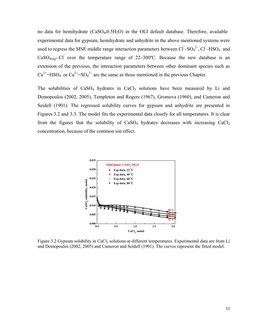
53

no data for hemihydrate (CaSO4.0.5H2O) in the OLI default database. Therefore, available

experimental data for gypsum, hemihydrate and anhydrite in the above mentioned systems were

used to regress the MSE middle range interaction parameters between Cl¯–SO42–, Cl¯–HSO4

¯ and

CaSO4(aq)–Cl¯ over the temperature range of 22–300ºC. Because the new database is an

extension of the previous, the interaction parameters between other dominant species such as

Ca2+−HSO4¯ or Ca2+−SO4

2− are the same as those mentioned in the previous Chapter.

The solubilities of CaSO4 hydrates in CaCl2 solutions have been measured by Li and

Demopoulos (2002, 2005), Templeton and Rogers (1967), Gromova (1960), and Cameron and

Seidell (1901). The regressed solubility curves for gypsum and anhydrite are presented in

Figures 3.2 and 3.3. The model fits the experimental data closely for all temperatures. It is clear

from the figures that the solubility of CaSO4 hydrates decreases with increasing CaCl2

concentration, because of the common ion effect.

0.0 0.5 1.0 1.5 2.00.000

0.005

0.010

0.015

0.020

0.025

0.030

0.035

80 oC60 oC40 oC

CaS

O4 so

lubi

lity,

mol

al

CaCl2, molal

Solid phase: CaSO4.2H2O

Exp data, 22 oC Exp data, 40 oC Exp data, 60 oC Exp data, 80 oC

22 oC

Figure 3.2 Gypsum solubility in CaCl2 solutions at different temperatures. Experimental data are from Li and Demopoulos (2002, 2005) and Cameron and Seidell (1901). The curves represent the fitted model.

54

0.0 0.5 1.0 1.5 2.0 2.5 3.0 3.5 4.00.000

0.005

0.010

0.015

0.020

0.025

0.030

0.035

0.040

0.045

0.050

50 oC80 oC110 oC

CaS

O4 so

lubi

lity,

mol

al

CaCl2, molal

Solid phase: CaSO4 (s)

Exp data, 25 oC Exp data, 50 oC Exp data, 80 oC Exp data, 110 oC Exp data, 250 oC Exp data, 300 oC

25 oC

Figure 3.3 Anhydrite solubility in CaCl2 solutions at different temperatures. Experimental data are from Li and Demopoulos (2005), Templeton and Rogers (1967), Gromova (1960). Curves are the fitted model.

The CaSO4–HCl–H2O system was studied by Li and Demopoulos (2002, 2005), Gupta (1968)

and is also cited by Linke and Seidell (1958) and Silcock (1979) in their solubility data

compilations over the temperature range of 10–80ºC. As shown in Figures 3.4 to 3.6, the model

fits the experimental data closely at all temperatures and for all three CaSO4 hydrates.

0 1 2 3 4 50.0

0.1

0.2

0.3

0.4

0.5

0.6

0.7

80 oC

60 oC

40 oC

22 oC

CaS

O4 so

lubi

lity,

mol

al

HCl, molal

Solid phase: CaSO4.2H

2O

Exp data, 22 oC Exp data, 40 oC Exp data, 60 oC Exp data, 80 oC

Figure 3.4 Gypsum solubility as a function of HCl concentration. Experimental data are from Li and Demopoulos (2002, 2005), Gupta (1968), Linke and Seidell (1958), Silcock (1979). Curves represent the fitted model.

0.00 0.02 0.04 0.06 0.08 0.10 0.12 0.14 0.16 0.180.0000

0.0002

0.0004

0.0006

0.0008

0.0010

300 oC

250 oC

55

The solubility of gypsum and anhydrite increases with increasing HCl concentration in the

range of 0.0–3.0 molal due to the formation of bisulphate ions which reduces the SO42-

concentration and allows an increase in the solubility of CaSO4 to satisfy the solubility product.

This effect is nullified at higher HCl concentrations due to the salting-out effect.

0 1 2 3 4 5 60.0

0.1

0.2

0.3

0.4

0.5

0.6

60 oC

80 oC

40 oC

CaS

O4 so

lubi

lity,

mol

al

HCl, molal

Solid phase: CaSO4

Exp data, 25 oC Exp data, 40 oC Exp data, 60 oC Exp data, 80 oC

25 oC

Figure 3.5 Anhydrite solubility in aqueous HCl solutions; experimental data are from Li and Demopoulos (2005), and curves represent the fitted model.

8.5 9.0 9.5 10.0 10.5 11.00.00

0.05

0.10

0.15

0.20

0.25

0.30

0.35

0.40

CaS

O4 so

lubi

lity,

mol

al

HCl, molal

Solid phase: CaSO4.1/2H

2O

Exp data, 25 oC Exp data, 50 oC

Figure 3.6 Hemihydrate solubility in aqueous HCl solutions; experimental data are from Li and Demopoulos (2005), and lines are the fitted model.

Similarly, the solubility of CaSO4 hydrates in aqueous solutions of NaCl was studied by

Templeton and Rogers (1967), Marshall and Slusher (1966), Ostroff and Metler (1966),

Marshall et al. (1964), Bock (1961) and also cited by Linke and Seidell (1958) and Silcock

56

(1979) in their solubility data compilations over the temperature range of 10–300ºC. The fitted

model results for the solubility of gypsum, anhydrite and hemihydrate in this ternary solution

are shown in Figures 3.7 to 3.9.

0.0 0.5 1.0 1.5 2.0 2.5 3.0 3.5 4.00.01

0.02

0.03

0.04

0.05

0.06

CaS

O4 so

lubi

lity,

mol

al

NaCl, molal

Solid phase: CaSO4.2H

2O

Exp data, 25 oC Exp data, 50 oC Exp data, 70 oC Exp data, 95 oC

Figure 3.7 Gypsum solubility in aqueous NaCl solutions. Experimental data are from Marshall and Slusher (1966), Ostroff and Metler (1966), Marshall et al. (1964), Linke and Seidell (1958), Silcock (1979); curves represent the fitted model.

0.0 0.5 1.0 1.5 2.0 2.5 3.0 3.5 4.0 4.50.00

0.02

0.04

0.06

0.08

0.10

0.12

0.14

0.16

250 oC175 oC125 oC

50 oC

CaS

O4 so

lubi

lity,

mol

al

NaCl, molal

Solid phase: CaSO4

Exp data, 25 oC Exp data, 50 oC Exp data, 125 oC Exp data, 175 oC Exp data, 250 oC

25 oC

Figure 3.8 Anhydrite solubility in aqueous NaCl solutions; experimental data are from Templeton and Rogers (1967), Marshall et al. (1964), Bock (1961) and Silcock (1979); curves represent the fitted model.

The solubility of all three solid phases increases slightly with increasing NaCl at low

concentrations due to the complexation effect of chloride ions and formation of calcium chloride

complexes (Williams-Jones and Seward, 1989).

57

0.0 0.5 1.0 1.5 2.0 2.5 3.0 3.5 4.00.00

0.02

0.04

0.06

0.08

0.10

CaS

O4 so

lubi

lity,

mol

al

NaCl, molal

Solid phase: CaSO4.1/2H2O

Exp data, 125 oC

Figure 3.9 Hemihydrate solubility as a function of NaCl concentration in aqueous solutions. Experimental data are from Marshall et al. (1964), and the curve represents the fitted model.

Cameron and Seidell (1901), Templeton and Rogers (1967), Ostroff and Metler (1966), and

Zdanovskii and Chernova (1976) measured the solubility of CaSO4 in the CaSO4–MgCl2–H2O

system from 25°C to 250ºC. Linke and Seidell (1958) also presented some data on this system

in their solubility data compilation. These data were also used, in addition to the experimental

data mentioned above (i.e., the solubility of all three CaSO4 hydrates in aqueous solutions of

CaCl2 and HCl, as well as in solutions of NaCl) to obtain interaction parameters between

Cl¯−SO42–, Cl¯−HSO4

¯ and CaSO4(aq)− Cl¯.

3.3.1.3 CaSO4–AlCl3–H2O System

The solubility of gypsum in aqueous AlCl3 solutions was measured by Li and Demopoulos

(2006a) from 25°C to 80°C. Additional fitting was performed on this system to attain the

interaction parameters between the AlSO4+−Ca2+ and Al3+−Ca2+ species (Appendix B). As is

clear from Figure 3.10, the obtained fits are in good agreement (AARD%=4.6) with the

experimental data. The solubility of gypsum first increases with increasing AlCl3 concentration

due to the complexation effect of chloride ions, however, at higher concentrations of AlCl3

(above 1 molal), this effect in nullified because of the decreased number of free water molecules

to participate in the dissolution process (the salting-out effect).

58

0.0 0.2 0.4 0.6 0.8 1.0 1.20.00

0.05

0.10

0.15

0.20

0.25

0.30

0.35

80 oC

50 oC

CaS

O4 so

lubi

lity,

mol

al

AlCl3, molal

Solid phase: CaSO4.2H

2O

Exp data, 25 oC Exp data, 50 oC Exp data, 80 oC

25 oC

Figure 3.10 Gypsum solubility in aqueous AlCl3 solutions. Experimental data are from Li and Demopoulos (2006a) and curves represent the fitted model.

3.3.1.4 CaSO4–FeCl3–HCl–H2O System

The solubility of gypsum in aqueous solutions containing FeCl3 and HCl (0.5 and 3.0 mol/L)

was measured by Li and Demopoulos (2006a). For this system, the MSE middle-range

interaction parameters between Ca2+ and FeCl2+ were regressed using the experimental data on

the solubility of gypsum in FeCl3 and 0.5 M of HCl system. Then, the obtained parameters were

employed to predict (without further regression) gypsum solubility in aqueous solutions

containing FeCl3 and 3 M of HCl. Figures 3.11 and 3.12 present regressed and predicted results

for these systems along with the experimental data, which are in good agreement.

0.0 0.5 1.0 1.5 2.0 2.50.00

0.05

0.10

0.15

0.20

0.25

0.30

0.35

0.40

80 oC

CaS

O4 so

lubi

lity,

mol

al

FeCl3, molal

Solid phase: CaSO4.2H2O

Exp data, 50 oC Exp data, 80 oC

[HCl]=0.5 M

50 oC

Figure 3.11 Gypsum solubility vs. FeCl3 concentration in CaSO4–FeCl3–HCl–H2O solutions. Experimental data are from Li and Demopoulos (2006a); curves represent the fitted model.

59

0.0 0.5 1.0 1.5 2.0 2.5 3.00.00

0.05

0.10

0.15

0.20

0.25

0.30

0.35

0.40

0.45

0.50

0.55

20 oC

50 oC

CaS

O4 so

lubi

lity,

mol

al

FeCl3, molal

Solid phase: CaSO4.2H

2O

Exp data, 20 oC Exp data, 50 oC

[HCl]=3 M

Figure 3.12 Gypsum solubility vs. FeCl3 concentration in CaSO4–FeCl3–HCl–H2O solutions. Experimental data are from Li and Demopoulos (2006a), and curves represent the predicted values.

3.3.2 Industrial Implications of the Model in Nickel Hydrometallurgy

As indicated in the previous section, the MSE activity coefficient model is effective for fitting

the solubility behaviour of the three solid phases of CaSO4 (gypsum, hemihydrate and

anhydrite) in mixed chloride-sulphate media. In order to validate the model parameters, the

solubilities of CaSO4 hydrates were calculated in multicomponent mixed chloride-sulphate

nickel hydromet processing solutions, containing NiSO4, Fe2(SO4)3, H2SO4, Na2SO4, and LiCl.

As will be seen later in this section, the model containing newly regressed parameters accurately

predicts (without additional fitting) the solubility behaviour of calcium sulphate in the systems

studied.

3.3.2.1 CaSO4–H2SO4–Fe2(SO4)3 (0.2 M)–NiSO4 (1.3 M)–LiCl (0.3 M)–H2O System

The effect of H2SO4 concentration from 0.0 to 0.7 mol/L, the maximum range of acid

concentration anticipated in the Voisey’s Bay Hydrometallurgical process, on the solubility of

calcium sulphate in simulated nickel sulphate-chloride processing solutions containing NiSO4,

H2SO4, Fe2(SO4)3 and LiCl at 25–95°C was studied by Dutrizac and Kuiper (2006). Figure 3.13

presents the experimental data and the solubilities predicted by the model. As is clear, the model

predictions are in good agreement with the experimental data (AARD%=8.0). Acid

concentration has a relatively minor effect on the solubility of CaSO4 in solutions containing 1.3

M NiSO4, 0.2 M Fe2(SO4)3 and 0.3 M LiCl. This dependence is due to the fact that the calcium

60

sulphate solubility in this system is mostly affected by the concentration of total free sulphate

ions released from dissociation of NiSO4 and Fe2(SO4)3. As a result, the presence of modest

concentrations of H2SO4 does not change the solubility of CaSO4 significantly. In this system,

gypsum was consistently the saturating solid phase in the experiments carried out using acid

concentrations less than 0.2 M H2SO4. But at higher acid concentrations, gypsum transformed

into anhydrite at temperatures above 90°C, with a consequential abrupt decrease in the solubility

of calcium sulphate.

0.0 0.1 0.2 0.3 0.4 0.5 0.6 0.7 0.8 0.90.00

0.01

0.02

0.03

0.04

0.05

0.06

0.07

90 oC

60 oC

[Fe2(SO4)3]=0.2M[NiSO

4]=1.3 M

[LiCl]=0.3 M

CaS

O4 so

lubi

lity,

mol

al

H2SO

4, molal

Solid Phase: CaSO4.2H

2O

Exp data, 30 oC Exp data, 60 oC Exp data, 90 oC

30 oC

Figure 3.13 CaSO4 solubility vs. H2SO4 concentration in CaSO4–H2SO4–Fe2(SO4)3(0.2M)–NiSO4(1.3M)–LiCl(0.3M)–H2O solutions. Experimental data are from Dutrizac and Kuiper (2006). Curves represent the predicted values.

3.3.2.2 CaSO4–Fe2(SO4)3–H2SO4 (0.15 M)–NiSO4 (1.3 M)–LiCl (0.3 M)–H2O System

In nickel pressure leaching processes, iron is dissolved in the autoclave along with nickel.

Although most of the dissolved iron re-precipitates in the autoclave as ferric oxide, ferric

oxyhydroxide or jarosite, some remains in the discharged solution. The dissolved iron is

subsequently oxidized and precipitated when the solution is neutralized with lime. Thus, various

iron concentrations are encountered in different parts of the process, for this reason, the effect of

the concentration of ferric sulphate on the solubility of calcium sulphate is important.

The solubility of CaSO4 as a function of ferric sulphate concentration in solutions containing 1.3

M NiSO4, 0.15 M H2SO4 and 0.3 M LiCl was also measured by Dutrizac and Kuiper (2006).

The predicted results obtained for the solubility of CaSO4 vs. Fe2(SO4)3 concentration are shown

61

in Figure 3.14 along with the experimental data. The model predictions accurately reflect the

experimental data (AARD%=4.3). Generally, the presence of ferric sulphate in the solution has

only a modest effect on the solubility of CaSO4. At 90°C, increasing Fe2(SO4)3 concentrations

causes a slight increase in the solubility of calcium sulphate, whereas at 30 and 60°C, solubility

is nearly independent of the concentration of Fe2(SO4)3.

0.0 0.2 0.4 0.6 0.8 1.00.00

0.01

0.02

0.03

0.04

0.05

0.06

0.07

0.08

30 oC

60 oC

[H2SO

4]=0.15 M

[NiSO4]=1.3 M

[LiCl]=0.3 M

Solid phase: CaSO4.2H

2O

Exp data, 30 oC Exp data, 60 oC Exp data, 90 oC

CaS

O4 so

lubi

lity,

mol

al

Fe2(SO

4)

3, molal

90 oC

Figure 3.14 CaSO4 solubility vs. Fe2(SO4)3 concentration in CaSO4–Fe2(SO4)3–NiSO4(1.3M)–H2SO4 (0.15M)–LiCl(0.3M)–H2O solutions; experimental data are from Dutrizac and Kuiper (2006), and curves represent the predicted values.

3.3.2.3 CaSO4–NiSO4–Fe2(SO4)3 (0.2 M)–H2SO4 (0.15 M)–LiCl (0.3 M)–H2O System

In the Voisey’s Bay Hydrometallurgical process, the maximum concentration of NiSO4 is

anticipated to be around 1.4 mol/L. Dutrizac and Kuiper (2006) studied the effect of NiSO4

concentration from 0.0 to 1.4 mol/L on the solubility of calcium sulphate in nickel sulphate-

chloride processing solutions containing 0.15 M H2SO4, 0.2 M Fe2(SO4)3, and 0.3 M LiCl at 25–

95°C. Figure 3.15 presents the experimental data along with the model predictions. The

predicted results are in good agreement with the experimental data (AARD%=6.1). The

solubility of calcium sulphate initially decreases with increasing NiSO4 concentration up to

0.2 M because of the common ion effect. This effect is diminished at higher NiSO4

concentrations (above 0.2 M) because of the association of Ca2+ and SO42- and formation of

calcium sulphate neutral species.

62

0.0 0.2 0.4 0.6 0.8 1.0 1.2 1.40.00

0.02

0.04

0.06

0.08

0.10

0.12

30 oC60 oC

[Fe2(SO4)3]=0.2M[H2SO4]=0.15 M[LiCl]=0.3 M

CaS

O4 so

lubi

lity,

mol

al

NiSO4, molal

Solid Phase: CaSO4.2H2O

Exp data, 30 oC Exp data, 60 oC Exp data, 90 oC

90 oC

Figure 3.15 CaSO4 solubility vs. NiSO4 concentration in CaSO4–NiSO4–Fe2(SO4)3(0.2M)–H2SO4 (0.15M)–LiCl(0.3M)–H2O solutions; experimental data are from Dutrizac and Kuiper (2006), and curves represent the model results.

3.3.2.4 CaSO4–LiCl–H2SO4 (0.15 M)–NiSO4 (1.3 M)–Fe2(SO4)3 (0.2 M)–H2O System

The addition of chloride ions to a sulphate processing solution could affect the solubility of

calcium sulphate. To ascertain the influence of chloride concentration on the solubility of

calcium sulphate, a systematic series of solubility measurements was carried out by Dutrizac

and Kuiper (2006) at various temperatures from 30°C to 90°C in solutions containing 1.3 M

NiSO4, 0.15 M H2SO4 and 0.2 M Fe2(SO4)3. LiCl was used as the chloride source, rather than

NaCl, to avoid the precipitation of sodium jarosite at temperatures above 80°C.

The experimental solubility data for this system are shown in Figure 3.16 along with the model

predictions for the system. As can be seen, the agreement is good at all temperatures studied

(AARD%=5.6). Also, it is clear that the solubility of CaSO4 decreases slightly as the

concentration of chloride ions in the solution increases because of the salting-out effect. At zero

concentration of LiCl, the solution already contains 1.3 M NiSO4, 0.2 M Fe2(SO4)3 and 0.15 M

H2SO4. Addition of other electrolytes (such as LiCl) results in a reduction in the number of free

water molecules participating in the dissolution process because they are tightly held by cations

and anions in the solution.

63

0.0 0.2 0.4 0.6 0.8 1.0 1.20.00

0.01

0.02

0.03

0.04

0.05

0.06

0.07

90 oC

60 oC

[Fe2(SO

4)

3]=0.2 M

[H2SO

4]=0.15 M

[NiSO4]=1.3 M

CaS

O4 so

lubi

lity,

mol

al

LiCl, molal

Solid Phase: CaSO4.2H

2O

Exp data, 30 oC Exp data, 60 oC Exp data, 90 oC

30 oC

Figure 3.16 CaSO4 solubility vs. LiCl concentration in CaSO4–LiCl–H2SO4(0.15M)–Fe2(SO4)3(0.2M)–NiSO4(1.3M)–H2O solutions; experimental data are from Dutrizac and Kuiper (2006), and curves represent the predicted values.

3.3.2.5 CaSO4–Na2SO4–H2SO4 (0.15 M)–NiSO4 (1.3 M)–LiCl (0.3 M)–H2O System

In nickel hydrometallurgy, sodium carbonate is sometimes used, directly or indirectly, for pH

control. This practice results in the presence of sodium ions in the circulating sulphate–chloride

processing solutions. The sodium ions can be considered to be present, formally, as either

Na2SO4 or NaCl. To investigate the effect of sodium ions on the solubility of calcium sulphate

in nickel sulphate–chloride processing solutions, at a constant chloride concentration, various

experiments were carried out by Dutrizac and Kuiper (2006) wherein Na2SO4 was added to the

simulated nickel processing solutions containing NiSO4, H2SO4 and LiCl.

The experimental data and the model predictions are shown in Figure 3.17, it is clear the model

closely predicts the solution chemistry (AARD%=4.9), without need for additional fitting. The

presence of modest concentrations of Na2SO4 in the 1.3 M NiSO4–0.15 M H2SO4–0.3 M LiCl

base solution has a minimal effect on the solubility of calcium sulphate at all temperatures

studied. This reflects the fact that calcium sulphate solubility is predominantly affected by the

total sulphate concentration. Accordingly, for concentrated NiSO4 solutions, the presence of the

modest concentrations (up to 0.5 M) of Na2SO4 does not affect the solubility of CaSO4

significantly.

64

0.0 0.1 0.2 0.3 0.4 0.5 0.60.00

0.01

0.02

0.03

0.04

0.05

0.06

0.07

90 oC

60 oC

[H2SO

4]=0.15 M

[NiSO4]=1.3 M

[LiCl]=0.3 M

CaS

O4 so

lubi

lity,

mol

al

Na2SO

4, molal

Solid Phase: CaSO4.2H2O

Exp data, 30 oC Exp data, 60 oC Exp data, 90 oC

30 oC

Figure 3.17 CaSO4 solubility vs. Na2SO4 concentration in CaSO4–Na2SO4–NiSO4(1.3M)–H2SO4(0.15M)–LiCl(0.3M)–H2O solutions; experimental data are from Dutrizac and Kuiper (2006), and curves represent the predicted values.

3.3.3 Predictive Capacity of the Model Parameters in Mixed Chloride Solutions

To further validate the predictive capacity of the model containing new interaction parameters,

the solubilities of calcium sulphate hydrates were calculated in multicomponent solutions

containing various chloride–sulphate electrolytes such as CaCl2, HCl, NaCl, MgCl2, Na2SO4,

and MgSO4 for which experimental data are available in the literature. As will be seen in the

following section, the model predictions are in good agreement with the experimental data

without performing additional fittings. This shows the usefulness of the model in predicting the

chemistry of complex systems for which no experimental data are available.

3.3.3.1 CaSO4–CaCl2–HCl–H2O System

The solubility of CaSO4 in mixed CaCl2 and HCl (1, 3, 5 M) aqueous solutions was measured

by Li and Demopoulos (2002, 2005) over the temperature range of 22–80°C. Silcock (1979)

also reported some data on this system in his solubility data compilation. Figures 3.18 to 3.20

show the experimental solubility data for all three solid phases of CaSO4 as a function of CaCl2

concentration at fixed HCl concentrations.

65

0.0 0.5 1.0 1.5 2.0 2.50.00

0.05

0.10

0.15

0.20

0.25

0.30

0.35

0.40

0.45

60 oC

40 oC

22 oC

[HCl]=6 M

CaS

O4 so

lubi

lity,

mol

al

CaCl2, molal

Solid phase: CaSO4.2H

2O

Exp data 22 oC Exp data 40 oC Exp data 60 oC

Figure 3.18 Gypsum solubility as a function of CaCl2 concentration in CaSO4–CaCl2–HCl–H2O solutions. Experimental data are from Li and Demopoulos (2002, 2005) and Silcock (1979); curves represent the predicted values.

0.0 0.5 1.0 1.5 2.0 2.5 3.0 3.5 4.0 4.50.00

0.02

0.04

0.06

0.08

0.10

0.12

0.14

0.16

50 oC80 oC

25 oC

[HCl]=6 M

CaS

O4 so

lubi

lity,

mol

al

CaCl2, molal

Solid phase: CaSO4

Exp data, 25 oC Exp data, 50 oC Exp data, 80 oC

Figure 3.19 Anhydrite solubility vs. CaCl2 concentration in CaSO4–CaCl2–HCl–H2O solutions; experimental data are from Li and Demopoulos (2005), and curves represent the predicted values.

Even at high concentrations of CaCl2 and HCl, the model closely predicts the solubility of all

three CaSO4 hydrates (AARD%=7.7 for 137 points). The trend shows that the addition of

calcium chloride to concentrated chloride solutions causes the solubility to decrease sharply

because of the common ion effect. Also, increasing HCl concentrations from 3 M to 6 M

reduces the number of free water molecules participating in the dissolution process, which

results in decreasing CaSO4 solubilities due to the salting-out effect.

66

0.0 0.5 1.0 1.5 2.0 2.5 3.0 3.5 4.0 4.50.00

0.05

0.10

0.15

0.20

0.25

0.30

0.35

0.40

0.45

0.50

[HCl]=3 M

[HCl]=6 M

CaS

O4 so

lubi

lity,

mol

al

CaCl2, molal

Solid phase: CaSO4.1/2H2O

Exp data, 60 oC Exp data, 80 oC

Figure 3.20 Hemihydrate solubility vs. CaCl2 concentration in CaSO4–CaCl2–HCl–H2O solutions; the experimental data are from Li and Demopoulos (2005), and curves represent the predicted values.

3.3.3.2 CaSO4–MgCl2–HCl–H2O System

Several experiments were carried out by Li and Demopoulos (2002, 2006a) to investigate the

effect of magnesium chloride concentration on the solubility of gypsum and anhydrite at

constant concentrations of hydrochloric acid, over the temperature range of 25–80°C. The

experimental solubility data for gypsum in this system at 3 M HCl are shown in Figure 3.21

along with the model predictions.

0.0 0.5 1.0 1.5 2.0 2.5 3.0 3.50.00

0.05

0.10

0.15

0.20

0.25

0.30

0.35

0.40

0.45

25 oC

[HCl]=3 M

CaS

O4 so

lubi

lity,

mol

al

MgCl2, molal

Solid Phase: CaSO4.2H

2O

Exp data, 25 oC Exp data, 50 oC

50 oC

Figure 3.21 Gypsum solubility vs. MgCl2 concentration in CaSO4–MgCl2–HCl–H2O solutions; the experimental data are from Li and Demopoulos (2006a), and curves represent the predicted values.

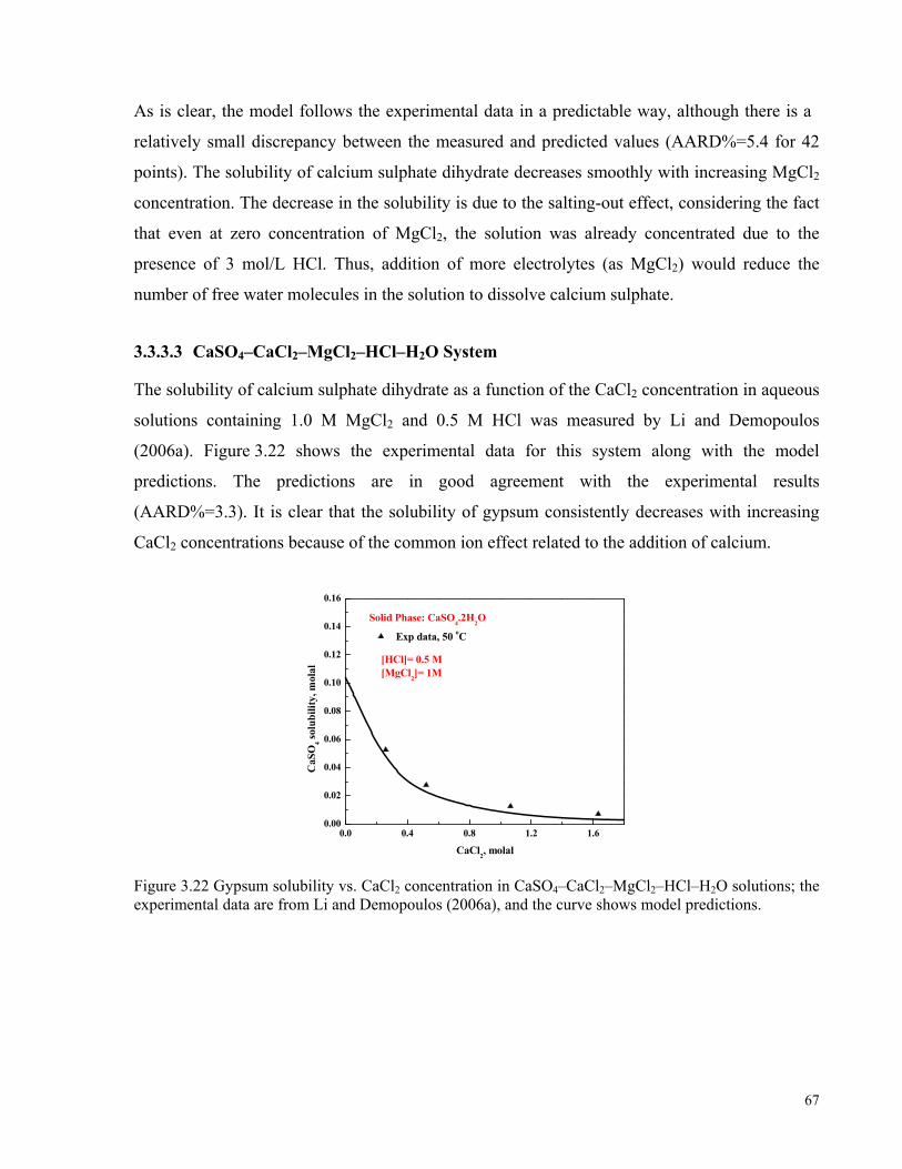
67

As is clear, the model follows the experimental data in a predictable way, although there is a

relatively small discrepancy between the measured and predicted values (AARD%=5.4 for 42

points). The solubility of calcium sulphate dihydrate decreases smoothly with increasing MgCl2

concentration. The decrease in the solubility is due to the salting-out effect, considering the fact

that even at zero concentration of MgCl2, the solution was already concentrated due to the

presence of 3 mol/L HCl. Thus, addition of more electrolytes (as MgCl2) would reduce the

number of free water molecules in the solution to dissolve calcium sulphate.

3.3.3.3 CaSO4–CaCl2–MgCl2–HCl–H2O System

The solubility of calcium sulphate dihydrate as a function of the CaCl2 concentration in aqueous

solutions containing 1.0 M MgCl2 and 0.5 M HCl was measured by Li and Demopoulos

(2006a). Figure 3.22 shows the experimental data for this system along with the model

predictions. The predictions are in good agreement with the experimental results

(AARD%=3.3). It is clear that the solubility of gypsum consistently decreases with increasing

CaCl2 concentrations because of the common ion effect related to the addition of calcium.

0.0 0.4 0.8 1.2 1.60.00

0.02

0.04

0.06

0.08

0.10

0.12

0.14

0.16

[HCl]= 0.5 M[MgCl

2]= 1M

CaS

O4 so

lubi

lity,

mol

al

CaCl2, molal

Solid Phase: CaSO4.2H

2O

Exp data, 50 oC

Figure 3.22 Gypsum solubility vs. CaCl2 concentration in CaSO4–CaCl2–MgCl2–HCl–H2O solutions; the experimental data are from Li and Demopoulos (2006a), and the curve shows model predictions.

68

3.3.3.4 CaSO4–Na2SO4–NaCl–H2O System

The solubility of gypsum and anhydrite in quaternary aqueous solutions of CaSO4, Na2SO4 and

NaCl, over the temperature range of 25–300°C, was determined by various researchers (Yeatts

and Marshall, 1972; Block and Waters, 1968; Furby et al., 1968; Templeton and Rodgers, 1967;

Cameron et al., 1907). It was shown that the solubility of gypsum first decreases sharply and

then increases gradually with increasing Na2SO4 concentration in the presence of up to 1 molal

NaCl. The initial decrease is due to the common ion effect of the added sulphate; the subsequent

increase is attributable to the association of Ca2+ and SO42- ions and formation of calcium

sulphate neutral species. For solutions containing 2.0 molal NaCl and above, the salting-out

effect becomes dominant, as a result, the increase in the solubility of gypsum is not observed

(Block and Waters, 1968; Templeton and Rodgers, 1967).

Similar trends are observed for the solubility of anhydrite, although solubilities are significantly

lower than those of gypsum at a given concentration of NaCl and Na2SO4. The new database,

utilized by the OLI/MSE model, is capable of making accurate predictions in these complex

systems (AARD%=6.5) as illustrated in Figures 3.23 and 3.24.

0.0 0.2 0.4 0.6 0.8 1.0 1.2 1.4 1.6 1.8 2.0 2.20.00

0.01

0.02

0.03

0.04

0.05

0.06

0.07

0.08

NaCl=4.0 mNaCl=2.0 m

NaCl=1.0 m

CaS

O4 so

lubi

lity,

mol

al

Na2SO

4, molal

Solid Phase: CaSO4.2H2O Exp data, [NaCl]=0.0 m Exp data, [NaCl]=1.0 m Exp data, [NaCl]=2.0 m Exp data, [NaCl]=4.0 m

NaCl=0.0 m

T= 40 oC

Figure 3.23 Gypsum solubility vs. Na2SO4 concentration in CaSO4–Na2SO4–NaCl–H2O solutions; the experimental data are from Block and Waters (1968), and the curves represent the predicted values.

69

0.00 0.05 0.10 0.15 0.20 0.25 0.300.0000

0.0005

0.0010

0.0015

0.0020

0.0025

0.0030

0.0035

0.0040

300 oC

250 oC

300 oC

I=0.5 m

CaS

O4 so

lubi

lity,

mol

al

Na2SO

4, molal

Solid phase: CaSO4

Exp data, 300 oC Exp data, 250 oC Exp data, 300 oC

I=0.9 m

Figure 3.24 Anhydrite solubility vs. Na2SO4 concentration in CaSO4–Na2SO4–NaCl–H2O solutions; the experimental data are from Templeton and Rodgers (1967), and curves represent the predicted values.

3.3.3.5 CaSO4–Na2SO4–MgCl2–H2O System

The solubility of gypsum in aqueous solutions of CaSO4, Na2SO4 and MgCl2 was measured by

Barba et al. (1984). Figure 3.25 shows the predicted results obtained from the model utilizing

the newly developed database compared with the experimental data. As can be seen, the model

predicts the experimental data closely (AARD%=8.0).

0.0 0.2 0.4 0.6 0.8 1.0 1.2 1.4 1.6 1.8 2.00.00

0.01

0.02

0.03

0.04

0.05

0.06

0.07

[MgCl2]=0.0 M

[MgCl2]=0.2 M

[MgCl2]=0.4 M

CaS

O4 so

lubi

lity,

mol

al

Na2SO

4, molal

Solid phase: CaSO4.2H

2O

Exp data, [MgCl2]=0.0 M Exp data, [MgCl2]=0.2 M Exp data, [MgCl2]=0.4 M Exp data, [MgCl2]=0.6 M

T=40 oC

[MgCl2]=0.6 M

Figure 3.25 Gypsum solubility vs. Na2SO4 concentration in CaSO4–Na2SO4–MgCl2–H2O solutions; the experimental data are from Barba et al. (1984), and curves represent the predicted values.

70

In this system, the solubility of calcium sulphate initially decreases with increasing Na2SO4

concentration at a fixed MgCl2 molality because of the common ion effect (SO42- is added and

the addition shifts the dissolution reaction to the left). However, for Na2SO4 concentrations

above ~0.4 molal, this effect is nullified by the association between Ca2+ and SO42− and the

consequential formation of calcium sulphate neutral species. Also, at a relatively low fixed

Na2SO4 concentration (below 0.4 molal) the solubility of gypsum increases with increasing

MgCl2 molality due to the complexation effect of chloride ions. However, the reverse trend is

observed for Na2SO4 concentrations above 0.4 molal where gypsum solubility decreases slightly

with increasing MgCl2 concentration due to the salting-out effect.

3.3.3.6 CaSO4–MgSO4–HCl–H2O / CaSO4–NiSO4–H2SO4–H2O Systems

To compare the effect of H2SO4 and HCl on the solubility of calcium sulfate, gypsum solubility

was measured in MgSO4 solutions containing 0.5 M HCl, as well as in NiSO4 solutions

containing 0.5 M H2SO4 in this work. The measured solubility data along with the model

prediction results from 25°C to 90°C are shown in Figures 3.26 and 3.27. Details regarding the

experimental procedure are discussed in Chapter 4.

0.0 0.2 0.4 0.6 0.8 1.0 1.2 1.4 1.60.00

0.05

0.10

0.15

0.20

0.25

0.30

Solid phase: CaSO4.2H

2O

Exp data, 25 oC Exp data, 45 oC Exp data, 70 oC Exp data, 90 oC

CaS

O4 so

lubi

lity,

mol

al

MgSO4, molal

[HCl]=0.5 M

Figure 3.26 CaSO4 solubility in CaSO4–MgSO4–HCl (0.5M)–H2O solutions; experimental data are from Azimi and Papangelakis (2010a), and curves are the model predictions.

In both systems, the solubility first decreases with increasing MSO4 (M=Ni, Mg) concentration

due to the common ion effect of the added SO42- ions. This effect is nullified by further

increasing MSO4 concentration because of the association of Ca2+ and SO42- ions and formation

of calcium sulfate neutral species. The solubility of gypsum is significantly higher in the

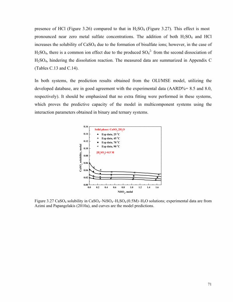
71

presence of HCl (Figure 3.26) compared to that in H2SO4 (Figure 3.27). This effect is most

pronounced near zero metal sulfate concentrations. The addition of both H2SO4 and HCl

increases the solubility of CaSO4 due to the formation of bisulfate ions; however, in the case of

H2SO4, there is a common ion effect due to the produced SO42- from the second dissociation of

H2SO4, hindering the dissolution reaction. The measured data are summarized in Appendix C

(Tables C.13 and C.14).

In both systems, the prediction results obtained from the OLI/MSE model, utilizing the

developed database, are in good agreement with the experimental data (AARD%= 8.5 and 8.0,

respectively). It should be emphasized that no extra fitting were performed in these systems,

which proves the predictive capacity of the model in multicomponent systems using the

interaction parameters obtained in binary and ternary systems.

0.0 0.2 0.4 0.6 0.8 1.0 1.2 1.4 1.60.00

0.02

0.04

0.06

0.08

0.10

0.12

0.14

0.16

[H2SO4]=0.5 M

CaS

O4 so

lubi

lity,

mol

al

NiSO4, molal

Solid phase: CaSO4.2H2O

Exp data, 25 oC Exp data, 45 oC Exp data, 70 oC Exp data, 90 oC

Figure 3.27 CaSO4 solubility in CaSO4–NiSO4–H2SO4 (0.5M)–H2O solutions; experimental data are from Azimi and Papangelakis (2010a), and curves are the model predictions.

72

3.4 Summary

The recently developed database for the mixed-solvent electrolyte (MSE) model on calcium

sulphate chemistry in sulphate electrolyte solutions was extended to be applicable in complex

multicomponent chloride-sulphate solutions. To improve the predictive capacity and self-

consistency of the new model, interaction parameters were obtained by fitting the experimental

data for ternary systems, and the interaction parameters were subsequently validated in

multicomponent systems. This approach is superior to that taken in other studies, wherein

interaction parameters were adjusted using multicomponent solutions, because the latter

approach does not guarantee consistent and accurate results in binary, ternary and other

multicomponent systems. The fact that modelling in binary and ternary systems is sufficient to

predict the behaviour of more complex multicomponent systems is a substantive contribution to

the existing field.

The new database, utilized by the OLI/MSE model, accurately predicts the solubility of calcium

sulphate, and therefore the scaling potential, in the neutralization stage of nickel sulphate-

chloride processing solutions of the Voisey’s Bay hydrometallurgical plant, containing NiSO4,

Fe2(SO4)3, Na2SO4, H2SO4, and LiCl at 20–95°C. The model was also shown to successfully

predict the solubilities of all three phases of calcium sulphate (DH, HH and AH) in mixed

chloride-sulphate solutions containing HCl, Ca, Fe(III), Mg, Na, and SO42- and over wide ranges

of temperature and composition. These facts illustrate the usefulness of the model in gaining

comprehensive insight for process improvements and optimization of conditions. The developed

database is utilized by mining companies such as Vale Inco to assess calcium sulphate scaling

potential in processing streams over wide ranges of temperature and concentration.

73

CHAPTER 4 SOLUBILITY OF GYPSUM AND ANHYDRITE IN LATERITE PRESSURE ACID LEACH SOLUTIONS

he focus of this chapter is on the experimental measurements of the solubility of gypsum

at 25–90°C and that of anhydrite at 150–250°C in simulated laterite pressure acid leach

(PAL) solutions. In this chapter, the predictive capacity of the model, utilizing the developed

database, was tested against the measured experimental data for both solids over wide ranges of

composition and temperature. This chapter is based on the following publication:

- Azimi, G., Papangelakis, V.G., 2010b. Hydrometallurgy, in press.

4.1 Introduction

In recent years, industrial processes at elevated temperatures have become of great interest. This

is particularly true in the hydrometallurgical nickel industry where sulphuric acid pressure

leaching of laterite ores has become the process of choice because of its fast kinetics, selective

extraction of valuable metals (Ni and Co) and simultaneous rejection of impurities (Al and Fe)

(Whittington and Muir, 2000).

Pressure acid leaching of the concentrate feed is carried out in autoclaves at high temperatures

between 150°C and 250°C. After digestion, the slurry is flashed to approximately 100°C and the

solids are separated from the liquid phase in a counter-current decantation (CCD) thickener

circuit. Most of impurities in the form of iron and aluminum initially present in the concentrate

feed precipitate in the autoclave, but a small amount remains in the discharged leach solution. In

order to increase the leach solution pH and precipitate the soluble impurities, the solution is

oxidized and subsequently neutralized by limestone (CaCO3). After filtration, the solution

containing the base metals is further treated by a number of methods including solvent

extraction and electrowinning to refine and extract the base metals from the solution. The

extracted metals are sent for further processing to recover pure metal or metal compound

products. The raffinate continues to a final neutralization stage to further increase pH and

precipitate the remaining metal ions, providing an environmentally safe solution for disposal.

The upstream process solution from the neutralization stage is saturated with gypsum at ambient

T

74

temperature and recycled to the beginning of the circuit for further usage. A process flow

diagram is presented in Chapter 1 (Figure 1.2).

The formation of undesirable calcium sulphate byproducts, mostly as scale, during pressure acid

leaching of laterite ores is one of the significant problems encountered in these processes. As

the scale layer becomes increasingly thicker, it reduces the production capacity and process

efficiency because of decreased volume of the equipment and reduced heat transfer capacity,

blocked pipelines and reduction of material flow, corrosion and wearing out of construction

materials. Also, calcium sulphate precipitation in the purification stage of base metals,

particularly in the solvent extraction stage, could create severe operational problems because of

the formation of a third solid phase (crud) (Nofal et al., 2001). Therefore, periodic shut-downs

of the plant for mechanical removal of precipitated calcium sulphate hydrates from the

processing circuit are necessary.

Calcium enters the sulphate refining electrolytes in different ways. Sometimes, the ore itself

contains calcium (Whittington and Muir, 2000). Also, the addition of calcium-containing bases

in the neutralization stage increases the concentration of calcium in the process circuit.

Moreover, in some refineries, the process water is a source of calcium ions. Calcium sulphate

hydrates (gypsum (CaSO4•2H2O), hemihydrate (CaSO4•0.5H2O) and anhydrite (CaSO4)) are

relatively insoluble and they are formed wherever calcium and sulphate occur together in

aqueous solutions. Many processes operate with very low solution bleeds and as a result,

calcium sulphate accumulates in the refining electrolyte. Furthermore, the transformation of

gypsum, the stable phase below 100°C, to anhydrite, the stable one at higher temperatures,

decreases the solubility significantly and makes the prediction and control of calcium sulphate

formation in these processes complicated. Therefore, having a thorough knowledge of the phase

behaviour of calcium sulphate and being able to accurately estimate the scaling potential in

these systems at various temperatures is of great practical importance.

A review of the literature reveals that no previous theoretical or experimental work has been

undertaken to study the simultaneous effects of coexisting metal sulphates and chlorides on the

solubility of CaSO4 hydrates over a broad temperature and concentration range in industrial

systems, particularly in laterite pressure acid leach (PAL) solutions. In terms of theoretical

modelling, most of the previous studies focused on CaSO4 solubility in water or in ternary and

75

quaternary aqueous solutions containing H2SO4, MgSO4, Na2SO4, etc. (Li and Demopoulos,

2006a; Arslan and Dutt, 1993; Barba et al., 1982).

A considerable amount of experimental work has been conducted to study calcium sulphate

solubilities under atmospheric pressure from 25°C to 95°C in water or in H2SO4 and HCl acidic

solutions as well as in multicomponent metal sulphate-chloride solutions (Farrah et al., 2007;

Dutrizac and Kuiper, 2006; Li and Demopoulos, 2005, 2006a; Dutrizac, 2002; Block and

Waters, 1968; Zdanovskii et al., 1968; Bock, 1961; Hill and Wills, 1938; Posnjak, 1938; Hulett

and Allen, 1902). At elevated temperatures, several experimental studies have also been

performed on solubility of calcium sulphate in water or in H2SO4 media as well as in ternary or

quaternary solutions containing NaCl, Na2SO4, MgCl2 up to 350°C (Blount and Dickson, 1969;

Furby et al., 1968; Marshall and Slusher, 1966, 1968; Templeton and Rodgers, 1967; Marshall

and Jones, 1966; Marshall et al., 1964; Partridge and White, 1929). However, no previous work

has been carried out to take into account the effect of metal sulphates on calcium sulphate

hydrates solubilities in multicomponent solutions over wide temperature ranges, particularly at

elevated temperatures, under acidic conditions.

In Chapters 2 and 3, a new database for the Mixed Solvent Electrolyte (MSE) model of the OLI

software was developed to predict calcium sulphate solubilities in multicomponent sulphate-

chloride electrolyte solutions (Azimi et al., 2007, 2008). The model was shown to accurately

predict gypsum and anhydrite solubility data in various industrial solutions including the nickel

sulphate-chloride processing solutions of the Voisey’s Bay plant (Azimi et al., 2008) and the

neutralized zinc sulphate leach solutions (Azimi et al., 2010) for which the experimental data

were measured by Dutrizac and Kuiper (2006) and Dutrizac (2002), respectively.

In this chapter, a number of experiments were conducted to measure the solubility of gypsum

and that of anhydrite in synthetic laterite pressure acid leach solutions containing NiSO4, H2SO4,

MgSO4, Al2(SO4)3 and NaCl in the respective temperature stability ranges, i.e., 25–90°C for

gypsum and 150–250°C for anhydrite. Then, the developed database, utilized by the OLI/MSE

model, was used to predict gypsum and anhydrite solubilities in the systems studied.

76

4.2 Experimental Procedure

All solutions used in this study were prepared by dissolving reagent grade chemicals directly

without further purification. Calcium sulphate dihydrate (gypsum) reagent was from J.T. Baker

with 99.4% purity and was used as one of the saturating solid phases. Calcium sulphate

anhydrite was also from J.T. Baker with 100% purity and was used as the other saturating solid

phase in this work. X-ray diffraction analysis was carried out on both solids using a Philips

PW3719 diffractometer. The diffractograms showed 100% gypsum and anhydrite, respectively

(Appendix D, Figures D.1 and D.2). No traces of hemihydrate or anhydrite were found in the

gypsum solid powder. For comparison purpose, the diffractogram of hemihydrate is also

presented in Appendix D.

Low temperature experiments under atmospheric pressure were performed inside 1 L double

layer reactors where heating was provided through a circulating oil jacket. Temperature was

controlled within ±1°C of the set-point. The reactor slurry was kept suspended by a shaft stirrer.

Samples were withdrawn through a dip tube using preheated syringes and filtrations were

performed using 0.22 μm PTFE syringe filters from Fisher Scientific. To avoid solution

evaporation during the runs, the stirrer bushings were fully sealed using Dow Corning® high

vacuum grease. Moreover, the concentration of elements other than Ca was monitored

throughout the experiments to confirm that the solution composition remained unchanged.

High temperature experiments were carried out in a 600 mL titanium autoclave, manufactured

by the Parr Instrument Company. Agitation was provided by a motor-driven titanium shaft

impeller. Temperature was controlled by manipulating an electrical heating mantle and a

cooling water stream, maintaining the autoclave temperature within ±1°C of the set-point. The

solution was placed inside a glass liner to protect the interior wall of the bomb from corrosion

and metal deposition. The autoclave was equipped with a dip tube for sample withdrawal

through an in situ 2 μm porous titanium filter. Schematic diagrams of the glass reactor and

autoclave are presented in Appendix E.

Solutions of known composition were placed in the reactors with an excess of saturating solid

phase. Experiments were started by heating the charged reactors to temperature and allowing

sufficient time to reach equilibrium while the reactor contents were agitated thoroughly.

77

Equilibration time in solubility measurements can vary over a wide range, from several hours

to several days, depending on the dissolution rate of the solid phase under the applied

conditions. In the present study, several kinetic tests were conducted at various temperatures and

the results showed that ~24 h was necessary to achieve complete saturation for low temperature

experiments, whereas 4–6 h was sufficient to reach equilibrium in high temperature experiments

inside the autoclave. In each test, two to three samples were taken towards the end of the run at

time intervals of 0.5–1 h to ensure that the calcium concentration reached a plateau as an

indication of equilibration.

Along with time-stable solubilities, the solubility data were also determined on heating and

cooling methods, based on dissolution and precipitation, as confirmatory indications of

equilibration. As long as the saturating solid phase remained unchanged, the various data

measured on heating and cooling were consistent. Reproducibility tests showed that the

experimentally measured data are accurate to within ±5%.

Withdrawn solution samples were diluted with 5% HNO3 and stored in sealed plastic test tubes

at room temperature. The Ca concentration was determined by ICP–OES analysis using the

317.933 nm emission line. The densities of the corresponding solutions were determined using a

portable density meter (DMA 35N) from Anton Paar. For the tests performed at temperatures

below 100°C, densities were measured “at temperature”, whereas for high temperature

experiments, they were measured at room temperature.

Samples of the equilibrating solid phase were also withdrawn, filtered, and washed with a small

amount of denatured alcohol, containing 85% ethanol and 15% methanol, to replace the solution

and dried below 40°C in an oven under vacuum. Powder X-ray diffraction patterns of the solid

samples were collected on a Philips PW3719 diffractometer utilizing Cu Ka radiation in the

range 10–60° 2θ with a step size of 0.02° and a collection time of 1.25 s/step. The generated

patterns were matched against the International Centre for Diffraction Data® files (JCPDF-

ICDD file numbers 070–0982 for gypsum and 072–0916 for anhydrite).

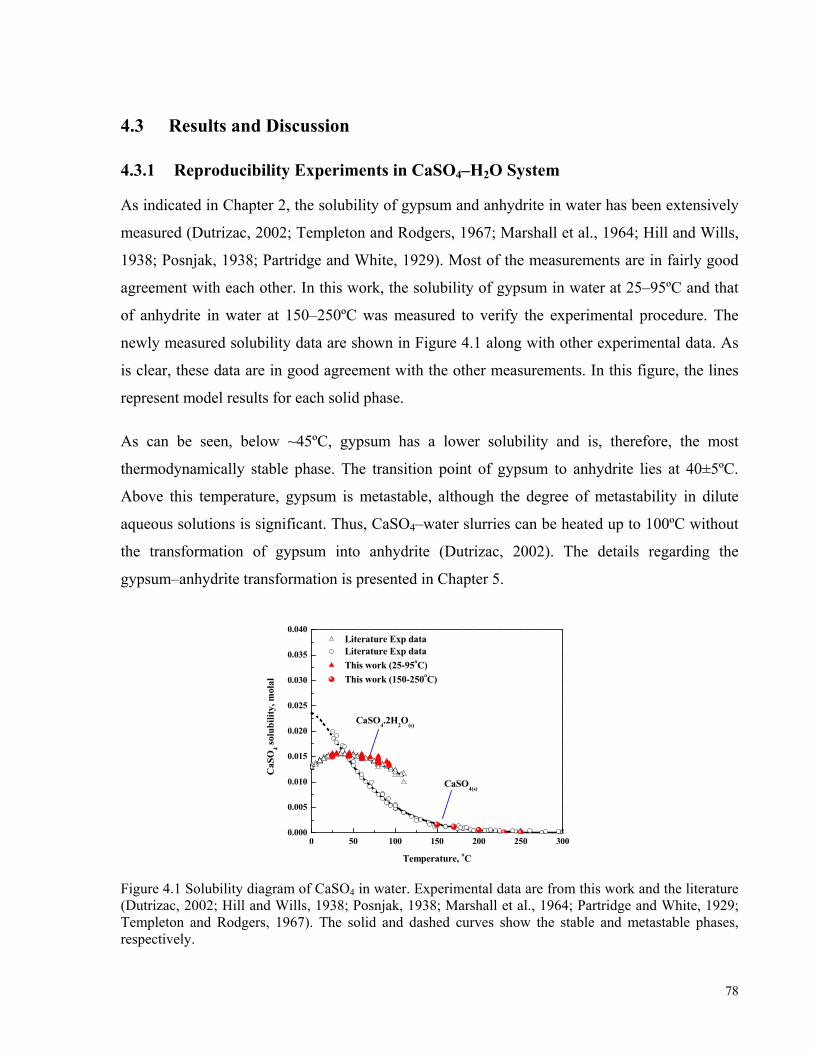
78

4.3 Results and Discussion

4.3.1 Reproducibility Experiments in CaSO4–H2O System

As indicated in Chapter 2, the solubility of gypsum and anhydrite in water has been extensively

measured (Dutrizac, 2002; Templeton and Rodgers, 1967; Marshall et al., 1964; Hill and Wills,

1938; Posnjak, 1938; Partridge and White, 1929). Most of the measurements are in fairly good

agreement with each other. In this work, the solubility of gypsum in water at 25–95ºC and that

of anhydrite in water at 150–250ºC was measured to verify the experimental procedure. The

newly measured solubility data are shown in Figure 4.1 along with other experimental data. As

is clear, these data are in good agreement with the other measurements. In this figure, the lines

represent model results for each solid phase.

As can be seen, below ~45ºC, gypsum has a lower solubility and is, therefore, the most

thermodynamically stable phase. The transition point of gypsum to anhydrite lies at 40±5ºC.

Above this temperature, gypsum is metastable, although the degree of metastability in dilute

aqueous solutions is significant. Thus, CaSO4–water slurries can be heated up to 100ºC without

the transformation of gypsum into anhydrite (Dutrizac, 2002). The details regarding the

gypsum–anhydrite transformation is presented in Chapter 5.

0 50 100 150 200 250 3000.000

0.005

0.010

0.015

0.020

0.025

0.030

0.035

0.040

CaSO4(s)

CaSO4.2H2O(s)

CaS

O4 so

lubi

lity,

mol

al

Temperature, oC

Literature Exp data Literature Exp data This work (25-95oC) This work (150-250oC)

Figure 4.1 Solubility diagram of CaSO4 in water. Experimental data are from this work and the literature (Dutrizac, 2002; Hill and Wills, 1938; Posnjak, 1938; Marshall et al., 1964; Partridge and White, 1929; Templeton and Rodgers, 1967). The solid and dashed curves show the stable and metastable phases, respectively.

79

4.3.2 Experimental Measurements and Model Predictions in Laterite PAL Solutions

Table 4.C in Appendix C shows the composition of a typical laterite PAL solution that would be

produced during the processing of a tropical limonite ore at 33% solids, containing about 0.7%

nickel, 1% magnesium and less than 3% aluminum, which was selected as a baseline in this

work. The effect of NiSO4, MgSO4 and H2SO4 concentrations on the solubility of gypsum and

anhydrite was investigated over their stability temperature ranges, which is 25–95°C for gypsum

and 150–250°C for anhydrite. Because seawater with various salinities has been used in the

Australian plants (Murrin Murrin, Ravensthorpe, Cawse and Bulong), the effect of NaCl

concentration on the solubility of calcium sulphate was also investigated in this work. As will be

seen later in this chapter, the model predicts the chemistry of CaSO4 hydrates in the systems

studied without performing additional fitting.

4.3.2.1 Effect of H2SO4 Concentration

The free acid concentration of leach solutions in the operating pressure acid leach processing

plants, which are the Cuban Moa Bay and the Australian Murrin Murrin processing plants,

ranges between 20–40 g/L (Whittington and Muir, 2000). Therefore, the effect of acid

concentration on the solubility of calcium sulphate is an important process parameter. Figures

4.2 and 4.3 present the measured solubility data for gypsum and anhydrite as a function of

H2SO4 concentration at different temperatures along with the model predictions. For both solids,

model predictions reflect the experimental data accurately. Tables C.5 and C.6 in Appendix C

summarize the measured data for gypsum and anhydrite, respectively. X-ray diffraction analysis

of the equilibrating solid phase showed gypsum at temperatures below 100°C and anhydrite at

150–250°C inside the autoclave.

As can be seen in Figure 4.2, at low temperatures (25–45°C), the addition of H2SO4 increases

the solubility of gypsum moderately, whereas at higher temperatures, the solubility increases

strongly with increasing acid concentration. The behaviour in dilute to moderately concentrated

acid is due to the decrease of the second dissociation constant of H2SO4 with increasing

temperature. Therefore, the addition of H2SO4 results in a reduction of the SO42- concentration

and allows an increase in the solubility of CaSO4 to satisfy the solubility product. Regardless of

the acid concentration, the solubility of gypsum increases monotonically with increasing

temperature. Figure 4.3 shows the solubility of anhydrite in similar solutions at elevated

80

temperatures. Under these conditions, anhydrite solubility increases significantly with

increasing acid concentration from 0.2 to 0.4 M. However, calcium sulphate solubility decreases

with increasing temperature. This is due to the fact that the dielectric constant of water decreases

with increasing temperature above 100°C, rendering water to be a deficient solvent for

dissolving polar compounds (Helgeson, 1967).

0.00 0.05 0.10 0.15 0.20 0.25 0.30 0.350.00

0.01

0.02

0.03

0.04

0.05

0.06

AARD%=7.5

Solid phase: CaSO4.2H2O

Exp data, 25 oC Exp data, 45 oC Exp data, 70 oC Exp data, 90 oC

CaS

O4 so

lubi

lity,

mol

al

H2SO

4, molal

[Al2(SO

4)

3]=0.004 M

[NiSO4]=0.07 M

[MgSO4]=0.23 M

Figure 4.2 Gypsum solubility vs. H2SO4 concentration in CaSO4–H2SO4–NiSO4(0.07M)–MgSO4(0.23M)–Al2(SO4)3(0.004M)–H2O solutions; experimental data are from Azimi and Papangelakis (2010b). The curves are the predicted values.

0.20 0.25 0.30 0.35 0.40 0.450.000

0.005

0.010

0.015

0.020

0.025

0.030

[Al2(SO4)3]=0.005 M[NiSO

4]=0.06 M

[MgSO4]=0.22 M

Solid phase: CaSO4 (s)

Exp data, 150 oC Exp data, 175 oC Exp data, 200 oC Exp data, 250 oC

CaS

O4 so

lubi

lity,

mol

al

H2SO

4, molal

AARD%=7.0

Figure 4.3 Anhydrite solubility vs. H2SO4 concentration in CaSO4–H2SO4–NiSO4(0.06M)–MgSO4(0.22M)–Al2(SO4)3(0.005M)–H2O solutions; experimental data are from Azimi and Papangelakis (2010b) and the curves are the model prediction results.

81

4.3.2.2 Effect of NiSO4 Concentration

In laterite pressure acid leach processes, the nickel concentration varies between 5 and 20 g/L.

The effect of this variation on the solubility of calcium sulphate in solutions containing

0.2–0.3 M H2SO4, 0.22 M MgSO4 and 0.005 M Al2(SO4)3 was investigated both at atmospheric

pressure at 25–90°C and at elevated pressures inside an autoclave at 150–250°C. X-ray

diffraction analysis showed gypsum as the saturating solid phase below 100°C and anhydrite

above 150°C. Figures 4.4 and 4.5 present the measured solubility data for gypsum and

anhydrite. It is clear from Figure 4.4 that the solubility of gypsum increases steadily with

increasing temperature due to the increase of the association constant (Ka) of CaSO4(aq) with

temperature. In contrast, as can be seen in Figure 4.5, the solubility of anhydrite decreases with

an increase in temperature above 150°C due to the reduction of the dielectric constant of water.

The measured data are presented in Appendix C (Tables C.7, C.8).

0.00 0.05 0.10 0.15 0.20 0.25 0.30 0.350.00

0.01

0.02

0.03

0.04

0.05

Solid phase: CaSO4.2H2O

Exp data, 25 oC Exp data, 45 oC Exp data, 70 oC Exp data, 90 oC

CaS

O4 so

lubi

lity,

mol

al

NiSO4, molal

[Al2(SO

4)

3]=0.005 M

[H2SO

4]=0.2 M

[MgSO4]=0.22 M

AARD%=5.4

Figure 4.4 Gypsum solubility vs. NiSO4 concentration in CaSO4–NiSO4–H2SO4(0.2M)–MgSO4(0.22M)–Al2(SO4)3(0.005M)–H2O solutions; experimental data are from Azimi and Papangelakis (2010b). The curves are the predicted values.

Both the solubility of gypsum and anhydrite first decreases moderately with increasing NiSO4

concentration due to the common ion effect. This effect is diminished at higher NiSO4

concentrations (above 0.2 M) due to the formation of calcium sulphate neutral species. The

MSE model containing the interaction parameters obtained in this work was used to predict the

solubility of both gypsum and anhydrite in these solutions over the temperature range studied.

The model predictions along with the experimental data are shown in Figures 4.4 and 4.5, which

are in good agreement (AARD%= 5.4 and 7.3).

82

0.05 0.10 0.15 0.20 0.25 0.30 0.350.000

0.004

0.008

0.012

0.016

[Al2(SO

4)

3]=0.005 M

[H2SO

4]=0.3 M

[MgSO4]=0.22 M

Solid phase: CaSO4

Exp data, 150 oC Exp data, 175 oC Exp data, 200 oC

CaS

O4 so

lubi

lity,

mol

al

NiSO4, molal

AARD%=7.3

Figure 4.5 Anhydrite solubility vs. NiSO4 concentration in CaSO4–NiSO4–H2SO4(0.3M)–MgSO4(0.22M)–Al2(SO4)3(0.005M)–H2O solutions; experimental data are from Azimi and Papangelakis (2010b). The curves are the predicted values.

4.3.2.3 Effect of MgSO4 Concentration

The concentration of MgSO4 in the laterite PAL solutions varies within the range of 0.05 to

0.5 M depending on the ore type (Baghalha, 1999). Limonitic ores contain low-Mg fractions

(about 1 wt%) compared to saprolite ores which contain high-Mg fractions between 10–20 wt%.

The variation in Mg content of laterite leach solutions has a significant impact on the solution

chemistry, particularly on the sulphuric acid consumption during the leaching process. This, in

turn, affects the Ni–Co leaching kinetics and the solubility of metal sulphates and impurities.

The impact of these variations on the solubility of calcium sulphate has not been studied before.

To provide some information on this aspect, the effect of MgSO4 on the solubilities of gypsum

and anhydrite in solutions containing 0.2–0.3 M H2SO4, 0.06 M NiSO4 and 0.005 M Al2(SO4)3

over the temperature range of 25–90°C and 150–250°C was investigated. The measured data are

summarized in Appendix C (Tables C.9, C.10). Saturating solid phases at all temperatures were

analyzed by X-ray diffraction. The results showed gypsum at temperatures below 100°C and

anhydrite above 150°C. Figure 4.6 shows the gypsum solubility data obtained at 25–90°C. In

this system, gypsum solubility first decreases as the MgSO4 concentration increases due to the

common ion effect; this effect is more pronounced at temperatures above 70°C. However, in the

presence of modest MgSO4 concentrations (above 0.25 M), the common ion effect is less

significant because of the association of Ca2+ and SO42- ions and formation of CaSO4(aq).

83

0.10 0.15 0.20 0.25 0.30 0.35 0.400.000

0.005

0.010

0.015

0.020

0.025

0.030

0.035

0.040

0.045[Al

2(SO

4)

3]=0.005 M

[H2SO

4]=0.2 M

[NiSO4]=0.05 M

Solid phase: CaSO4.2H

2O

Exp data, 25 oC Exp data, 45 oC Exp data, 70 oC Exp data, 90 oC

CaS

O4 so

lubi

lity,

mol

al

MgSO4, molal

AARD%=6.0

Figure 4.6 Gypsum solubility vs. MgSO4 concentration in CaSO4–MgSO4–H2SO4(0.2M)–NiSO4(0.05M)–Al2(SO4)3(0.005M)–H2O solutions; experimental data are from Azimi and Papangelakis (2010b). The curves are the predicted values.

The solubility of anhydrite over the temperature range of 150–250°C is presented in Figure 4.7.

Increasing MgSO4 concentration from 0.05 to 0.35 M in the solution containing 0.3 M H2SO4,

0.06 M NiSO4 and 0.005 Al2(SO4)3 results in a systematic decrease in the solubility due to the

common ion effect of SO42-. The model was used to predict the solubilities of both gypsum and

anhydrite in these systems over the temperature and concentration ranges studied. The curves

presented in Figures 4.6 and 4.7 are model prediction results which are in good agreement with

the measured data (AARD%=6.0 and 8.8).

0.10 0.15 0.20 0.25 0.30 0.350.000

0.005

0.010

0.015

0.020

0.025

0.030

0.035

[Al2(SO

4)

3]=0.005 M

[H2SO4]=0.3 M[NiSO

4]=0.06 M

Solid phase: CaSO4

Exp data, 150 oC Exp data, 175 oC Exp data, 200 oC Exp data, 250 oC

CaS

O4 so

lubi

lity,

mol

al

MgSO4, molal

AARD%=8.8

Figure 4.7 Anhydrite solubility vs. MgSO4 concentration in CaSO4–MgSO4–H2SO4(0.3M)–NiSO4(0.06M)–Al2(SO4)3(0.005M)–H2O solutions; experimental data are from Azimi and Papangelakis (2010b). The curves are the predicted values.

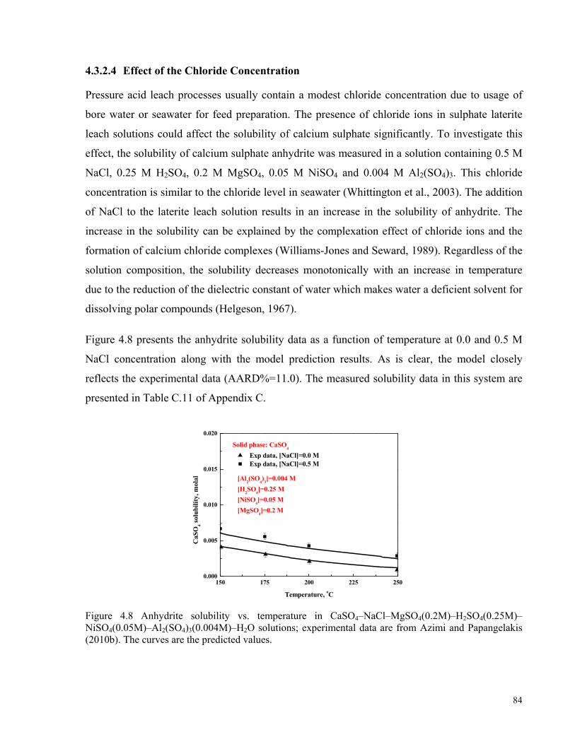
84

4.3.2.4 Effect of the Chloride Concentration

Pressure acid leach processes usually contain a modest chloride concentration due to usage of

bore water or seawater for feed preparation. The presence of chloride ions in sulphate laterite

leach solutions could affect the solubility of calcium sulphate significantly. To investigate this

effect, the solubility of calcium sulphate anhydrite was measured in a solution containing 0.5 M

NaCl, 0.25 M H2SO4, 0.2 M MgSO4, 0.05 M NiSO4 and 0.004 M Al2(SO4)3. This chloride

concentration is similar to the chloride level in seawater (Whittington et al., 2003). The addition

of NaCl to the laterite leach solution results in an increase in the solubility of anhydrite. The

increase in the solubility can be explained by the complexation effect of chloride ions and the

formation of calcium chloride complexes (Williams-Jones and Seward, 1989). Regardless of the

solution composition, the solubility decreases monotonically with an increase in temperature

due to the reduction of the dielectric constant of water which makes water a deficient solvent for

dissolving polar compounds (Helgeson, 1967).

Figure 4.8 presents the anhydrite solubility data as a function of temperature at 0.0 and 0.5 M

NaCl concentration along with the model prediction results. As is clear, the model closely

reflects the experimental data (AARD%=11.0). The measured solubility data in this system are

presented in Table C.11 of Appendix C.

150 175 200 225 2500.000

0.005

0.010

0.015

0.020

[Al2(SO

4)

3]=0.004 M

[H2SO4]=0.25 M[NiSO

4]=0.05 M

[MgSO4]=0.2 M

Solid phase: CaSO4

Exp data, [NaCl]=0.0 M Exp data, [NaCl]=0.5 M

CaS

O4 so

lubi

lity,

mol

al

Temperature, oC

Figure 4.8 Anhydrite solubility vs. temperature in CaSO4–NaCl–MgSO4(0.2M)–H2SO4(0.25M)–NiSO4(0.05M)–Al2(SO4)3(0.004M)–H2O solutions; experimental data are from Azimi and Papangelakis (2010b). The curves are the predicted values.

85

The solubility of gypsum as a function of NaCl concentration was also measured in solutions

containing 0.5 M H2SO4 at temperatures below 100°C. Table C.12 in Appendix C summarizes

these data. Similar to the high temperature results, gypsum solubility increases with increasing

the NaCl concentration due to the complexation effect of chloride ions. Figure 4.9 shows the

gypsum solubility as a function of NaCl concentration in comparison with the predicted results

obtained from the model. As can be seen, the model results are in good agreement with the

experimental data (AARD%=4.1).

0.0 0.2 0.4 0.6 0.8 1.0 1.2 1.4 1.60.00

0.03

0.06

0.09

0.12

0.15

0.18

CaS

O4 so

lubi

lity,

mol

al

NaCl, molal

Solid phase: CaSO4.2H

2O

Exp data, 25 oC Exp data, 45 oC Exp data, 70 oC Exp data, 90 oC

[H2SO

4]=0.5M

AARD%=4.1

Figure 4.9 Gypsum solubility vs. NaCl concentration in CaSO4–NaCl– H2SO4(0.5M)– H2O solutions; experimental data are from Azimi and Papangelakis (2010b). The curves are the predicted values.

4.4 Process Implications of the Results

The database developed in this work, utilized by the OLI/MSE model, was shown to accurately

predict the solubility behaviour of calcium sulphate (gypsum and anhydrite) in multicomponent

solutions containing Al2(SO4)3, H2SO4, MgSO4, NiSO4, and NaCl from ambient temperature to

250ºC. The model can be used as a valuable tool to map the behaviour of calcium sulphate in

aqueous industrial solutions and to assess the potential for scaling in various aqueous streams.

This, in turn, will provide different industries with the opportunity to investigate the effect of

different variables such as temperature and composition and aid them in finding solutions to

minimize scale formation in the processing circuits. The following implications can be drawn

from this study:

86

1. Calcium sulphate dihydrate (gypsum) is the practically stable solid phase below 100ºC,

due to slow kinetics of phase transformation, although the true upper temperature is

about 40ºC. Above 100ºC anhydrous calcium sulphate (anhydrite) becomes the stable

phase, and its solubility decreases with temperature because the dielectric constant of

water decreases with increasing temperature above 100°C (Helgeson, 1967).

2. The solubility of anhydrite is much lower than that of gypsum (approximately one order

of magnitude lower). As a result, process solutions which are saturated with gypsum at

ambient temperature and recycled to the autoclave need to be processed to decrease their

calcium content and make it less than the saturation level of anhydrite inside the

autoclave. This can be done by mixing the recycling stream with carbonate compounds

to reject calcium as calcium carbonate, provided that the solution is not acidic.

Otherwise, scale formation in the hot zones of the plants will be unavoidable. In fact,

such scaling issues have been reported in pre-heaters during the Bulong plant operation

(Nofal et al., 2001).

3. The addition of H2SO4 has a strong positive effect on the solubility of calcium sulphate

in water (up to 10 times increase) over the temperature range of 25–250ºC. The addition

of acid up to around 1.0–2.0 M increases the solubility of calcium sulphate hydrates due

to the formation of HSO4- ions. Above this concentration, calcium sulphate solubility

reaches a plateau, and upon further acid addition, the solubility decreases due to the

salting-out effect.

4. The addition of sulphate electrolytes such as NiSO4 and MgSO4 first has a negative

effect on the solubility of calcium sulphate due to the common ion effect. However, in

the presence of modest sulphate concentration (above 0.2–0.3 molal), this effect is

nullified due to the association of Ca2+ and SO42- ions and formation of calcium sulphate

neutral species which results in an increase in the solubility. After passing a maximum,

the solubility decreases at still higher sulphate concentrations (above ~1.5–2.0 molal) as

a result of the salting-out effect.

5. The solubility of gypsum in water reaches a maximum at ~45–50ºC, followed by a slight

decrease in the solubility at higher temperatures. However, in multicomponent process

solutions, gypsum is increasingly soluble with temperature. This effect is shown in

87

Figure 4.10 at different NiSO4 concentrations from 0.1 to 1.0 molal in comparison with

that in pure water. As can be seen, the solubility, which decreases with increasing

temperatures above ~40ºC in water, becomes positively related to temperature at high

sulphate concentrations. As a result, process solutions saturated with gypsum during a

hot upstream neutralization step have the potential for scale formation when cooled to

lower temperatures.

30 40 50 60 70 80 900.000

0.005

0.010

0.015

0.020

0.025

pure water

[NiSO4]=0.2 m

[NiSO4]=0.1 m

[NiSO4]=0.5 m

C

aSO

4 Sol

ubili

ty, m

olal

Temperature, oC

[NiSO4]=1 mSolid phase: CaSO4.2H2O

Figure 4.10 Gypsum solubility as a function of temperature at various NiSO4 concentrations in comparison with that in pure water; the curves are the model prediction results.

6. The addition of chloride ions (up to ~1.5–2.0 molal) increases the solubility of calcium

sulphate in the systems studied. Above this concentration, the solubility reaches a

plateau. The increase in the solubility is due to the complexation effect of the chloride

ions. However, this effect is less significant at higher salt concentrations due to the

salting-out effect. Figure 4.11 depicts the predicted anhydrite solubility in pure water as

well as in an aqueous solution of 0.22 M H2SO4 in comparison with that in laterite PAL

solutions containing 0.22 M H2SO4, 0.2 M MgSO4, 0.05 M NiSO4 and 0.005 M

Al2(SO4)3 at various chloride concentrations equivalent to those found in tap water,

seawater, saline and hyper–saline water (Whittington et al., 2003). For comparison, the

saturation level of gypsum in pure water at 25ºC is also presented. As is clear,

transformation between gypsum, the “practically” stable solid phase below 100ºC, and

anhydrite, the stable phase above 150ºC, results in a significant decrease (~90%) in the

solubility of calcium sulphate in pure water. However, the addition of H2SO4 has a

positive effect on the solubility of anhydrite in the solution. In this figure, anhydrite

88

solubility in a solution containing 0.22 M H2SO4 was increased by almost 70%

compared to that in pure water. In contrast, the addition of metal sulphates, i.e., MgSO4,

NiSO4 and Al2(SO4)3 results in a decrease in anhydrite solubility in 0.22 M H2SO4

solutions. The addition of chloride ions has a positive effect on the solubility of

anhydrite in the laterite PAL solutions.

150 175 200 225 2500.000

0.002

0.004

0.006

0.008

0.010

0.012

0.014

0.016

0.018

PALhypersaline, Cl-=74550 ppm

saline, Cl-=35500 ppmseawater, Cl-=18000 ppm

tapwater, Cl-=140 ppm

CaS

O4 so

lubi

lity,

mol

al

Temperature, oC

gypsum saturated water at 25 oC

anhydrite in pure water

in pure H2SO4=0.22 M

Figure 4.11 Anhydrite solubility vs. temperature in pure water and in 0.22 M H2SO4 solution in comparison with that in laterite PAL solutions containing MgSO4(0.2M)–H2SO4(0.22M)–NiSO4(0.05M)–Al2(SO4)3 (0.005M) at various chloride concentrations. Solid curves are model prediction results for anhydrite; the dashed line shows gypsum saturation level in pure water at 25°C.

7. To indicate the effect of H2SO4 concentration, the predicted anhydrite solubility in pure

water as well as in 0.22 M H2SO4 solutions along with that in laterite PAL solutions

containing 0.2 M MgSO4, 0.05 M NiSO4 and 0.005 M Al2(SO4)3 at three different H2SO4

concentrations, i.e., 0.22, 0.33, and 0.44 M are presented in Figure 4.12. The dashed line

represents the saturation level of gypsum in pure water at 25ºC. As discussed above, the

transformation of gypsum to anhydrite results in a ~90% decrease in the solubility of

CaSO4 in pure water. The addition of 0.22 M H2SO4 increases anhydrite solubility in

water by ~70%. However, in PAL solutions, the solubility decreases due to the common

ion effect. Increasing acid concentration from 0.22 M to 0.33 M results in ~60% increase

in the anhydrite solubility in PAL solutions at 250ºC. Therefore, higher acidities, higher

water salinity and lower sulphate concentrations are favorable conditions for minimizing

anhydrite scaling inside an autoclave. These parameters must be optimized to target

capital and operating costs, material consumption, and environmental regulations.

89

150 175 200 225 2500.000

0.002

0.004

0.006

0.008

0.010

0.012

0.014

0.016

0.018

PAL

PAL

[H2SO4]=0.44 M

[H2SO4]=0.33 M

PAL

CaS

O4 so

lubi

lity,

mol

al

Temperature, oC

gypsum saturated water at 25 oC

anhydrite in pure water

in pure H2SO4=0.22 M

[H2SO4]=0.22 M

Figure 4.12 Anhydrite solubility vs. temperature in pure water and in 0.22 M H2SO4 solutions compared to that in laterite PAL solutions containing MgSO4(0.2M)–NiSO4(0.05M)–Al2(SO4)3 (0.005M) at various H2SO4 concentrations. Solid curves are model prediction results for anhydrite; the dashed line shows gypsum saturation level in pure water at 25°C.

4.5 Summary

In hydrometallurgical processing of metals such as nickel, cobalt and copper, the limited

solubility of calcium sulphate results in very low concentrations of calcium in the circuit.

However, as the temperature and solution composition vary, calcium sulphate scaling may occur

in the process. During processing at higher temperatures, transformation between the calcium

sulphate hydrates has a complex effect on the solubility, making the behaviour of calcium

sulphate difficult to predict and control. Most of the industries dealing with calcium sulphate

scale formation employ regular removal of precipitated calcium sulphate because the build-up of

calcium concentration in these process streams is unavoidable.

The solubilities of gypsum and anhydrite in synthetic pressure acid leach solutions containing

NiSO4, H2SO4, Al2(SO4)3, and MgSO4 were measured from 25°C to 250ºC. Gypsum is the

stable solid phase at low temperatures; however, at high temperatures, above 100ºC, anhydrite

becomes the stable phase and its solubility decreases with temperature. Furthermore, the

solubility of anhydrite in pure water above 100ºC is roughly one tenth of that of dihydrate below

100ºC. Therefore, process solutions which are saturated with gypsum at room temperature and

recycled to the autoclave have the potential to form anhydrite scales. The addition of H2SO4 up

90

to ~2.0 M results in a significant increase in the solubility of both gypsum and anhydrite.

Above this concentration, calcium sulphate solubility decreases with increasing acid

concentration.

The addition of metal sulphates such as NiSO4, and MgSO4 has a negative effect on the

solubility of calcium sulphate hydrates in laterite PAL solutions over the temperature range

studied due to the common ion effect. It was also found that the quality of the process water

affects the solubility of CaSO4 in these solutions. The addition of chlorides from tap water

(~140 ppm) to hyper-saline water (~75000 ppm) increases the solubility of anhydrite by almost

20%. Therefore, mixing recycled process solutions with seawater is favorable for decreasing

anhydrite scale formation in these systems provided that chloride-corrosion issues can be

controlled by utilizing chloride-resistant materials and metal alloys.

The experimentally measured solubility data were successfully modelled using the newly

developed database utilized by the OLI/MSE model. The model was shown to accurately predict

the solubility behaviour of calcium sulphate in solutions under the conditions studied. The

model can be used to map calcium sulphate chemistry in the sulphuric acid pressure leaching of

laterite ores over wide ranges of temperature and concentration. This, in turn, results in a

comprehensive insight for process improvements and optimization.

91

CHAPTER 5 TRANSFORMATION OF GYPSUM INTO ANHYDRITE IN AQUEOUS ELECTROLYTE SOLUTIONS

his chapter focuses on the transformation of gypsum into anhydrite. The effect of

temperature, sulphuric acid concentration, anhydrite seeding as well as addition of

sulphate and chloride salts on the transformation kinetics is discussed. Based on the results

obtained, a mechanism for the gypsum–anhydrite transformation is proposed. The contents of

this chapter have been submitted to the Crystal Growth & Design for publication (Submission #:

cg-2010-00172b).

5.1 Introduction

Calcium sulphate dihydrate (CaSO4•2H2O) occurs naturally as the mineral gypsum and is the

most common sulphate mineral in the environment that has been traditionally extracted from the

ground (Hand, 1997). In the modern world, gypsum is widely used as a constituent in

construction materials such as cement or gypsum wallboards (Christensen et al., 2008; Solberg

et al., 2002) as well as in the production of biocompatible materials such as bone void fillers

(Doadrio et al., 2004). However, calcium sulphate appears as an undesirable byproduct, mostly

as discard solids and/or as scale, in many industrial processes including wastewater treatment,

oil and gas production, desalination, sulphur dioxide removal from coal-fired power plants flue

gas (Lee et al., 2006; Dathe et al., 2006) and during neutralization of free sulphuric acid in

hydrometallurgical processes (Azimi and Papangelakis, 2010b; Dutrizac and Kuiper, 2008,

2006; Adams and Papangelakis, 2007; Dutrizac, 2002). Calcium sulphate scale formation in

industrial plants results in reduced production capacity and process efficiency due to decreased

equipment volume, heat transfer capacity, and material flow, blocked pipelines and corrosion.

Therefore, periodic shut-downs of the plant for maintenance and mechanical removal of

precipitated calcium sulphate hydrates are necessary.

Five crystalline phases in the form of hydrates or polymorphs exist in the CaSO4–H2O system:

dihydrate or gypsum (CaSO4•2H2O, DH), hemihydrate in the two polymorphs of

α–CaSO4•0.5H2O and β–CaSO4•0.5H2O, and anhydrite in the two polymorphs of soluble and

T

92

insoluble, denoted as AIII or γ–CaSO4 and AII–CaSO4, respectively (Christensen et al., 2008).

The difference between polymorphs and hydrates is that polymorphs are different crystal

structures of the same stoichiometry, whereas, hydrates are crystals of a compound incorporated

with a different number of water molecules (Zupancic et al., 2005).

One of the most common causes of CaSO4 scale formation in various industries is the

transformation of gypsum into insoluble anhydrite (AII–CaSO4), as was the case with the

Bulong Nickel/Cobalt Plant (Nofal et al., 2001). Theoretically, gypsum is the stable solid phase

in water up to ~45–50°C, and above that it transforms into anhydrite (Farrah et al., 2004; Freyer

and Voigt, 2003; Dutrizac, 2002; Nývlt, 1997). However, the transformation does not practically

occur up to ~80–90°C due to the slow kinetics in the absence of anhydrite seeding. Because the

solubility of anhydrite is lower than that of gypsum, the transformation of gypsum into

anhydrite generates a supersaturated solution, which results in anhydrite scale formation. In

industrial practice, this means that during sulphuric acid neutralization with calcium-containing

bases, first gypsum forms as a metastable phase because of its higher solubility, according to the

Ostwald step rule (Santen, 1984), then gradually transforms into anhydrite. Thus, a thorough

understanding of the mechanism and kinetics of the solid phase transformation in addition to the

solution chemistry of CaSO4 is of great practical importance to accurately evaluate the scaling

potential in various electrolyte solutions.

The thermodynamics of transformation between gypsum and anhydrite in water at one

atmosphere has been studied by several researchers (Knacke and Gans, 1977; Hardie, 1967;

Power at al., 1964; Posnjak, 1938; Hill, 1937; Partridge and White, 1929; Van’t Hoff et al.,

1903). The effect of salt solutions on the gypsum–anhydrite transformation has also been

investigated (Ostroff, 1964; Bock, 1961; Posnjak, 1940; Hill and Wills, 1938; Van’t Hoff et al.,

1903). More recently, Li and Demopoulos (2006c) constructed thermodynamic phase diagrams

of calcium sulphate hydrates in HCl–CaCl2–H2O solutions up to 100°C and derived theoretical

stability regions of various hydrates as a function of temperature and composition. Most of these

studies have focused on the thermodynamics of transformation and determination of the

theoretical transition temperature between gypsum and anhydrite.

The kinetics of transformation between various calcium sulphate hydrates, particularly under the

conditions resembling those in industrial processes, has also been studied over the present

93

decade. Transformation of gypsum into anhydrite in hot acidic manganese sulphate solutions

has been studied by Farrah et al. (2004), where an autocatalytic process was suggested to fit the

transformation kinetics. The gypsum–anhydrite transformation in simulated nickel sulphate–

chloride and copper sulphate electrorefining solutions has also been studied by Dutrizac and

Kuiper (2006, 2008). In a recent study (Dutrizac, 2002) on the solubility of gypsum in sulphuric

acid solutions, it has been realized that the equilibration kinetic curves in the case of heating and

cooling were not coincident for H2SO4 concentrations above 0.6 M, i.e., the solubility increased

up to ~80–90°C and then dropped abruptly as a result of the transformation of gypsum into

anhydrite. In all previous studies, the concentration of sulphuric acid has been found to play an

important role in the kinetics of the transformation. That is, a higher acid concentration lowers

the time required to complete the transformation.

In the previous chapters, the solubilities of gypsum and anhydrite in various multicomponent

industrial systems was studied and a new database for the Mixed Solvent Electrolyte (MSE)

model of the OLI® software was developed, which is capable of predicting the solubility

behaviour (and hence the scaling potential) of CaSO4 in such processes up to 250°C (Azimi and

Papangelakis, 2010a, 2010b; Azimi et al., 2010, 2008, 2007). In this chapter, a systematic study

of the kinetics of gypsum–anhydrite transformation was carried out over the temperature range

of 25–90°C, which is the temperature range where neutralization processes occur in industry. A

number of experiments were conducted to study the effects of temperature, acid concentration

from 0.5 to 2.0 M, anhydrite seeding and addition of sulphate/chloride salts (NiSO4 and NaCl)

on the transformation kinetics. The transformation of gypsum into anhydrite was monitored

closely both in liquid and the solid phases.

5.2 Experimental Section

All solutions were prepared by dissolving reagent grade chemicals directly without further

purification. Gypsum reagent with 99.4% purity and anhydrite with 100% purity from J.T.

Baker were used as saturating solid phases. X-ray diffraction (XRD) analysis was carried out on

both solids. The diffractograms showed 100% gypsum and anhydrite, respectively (Appendix

D). No traces of hemihydrate or anhydrite were found in the gypsum solid powder.

Experiments were performed inside 1 L double layer glass reactors with tight-fitting lids where

heating was provided through a circulating oil jacket. Temperature was controlled within ±1°C

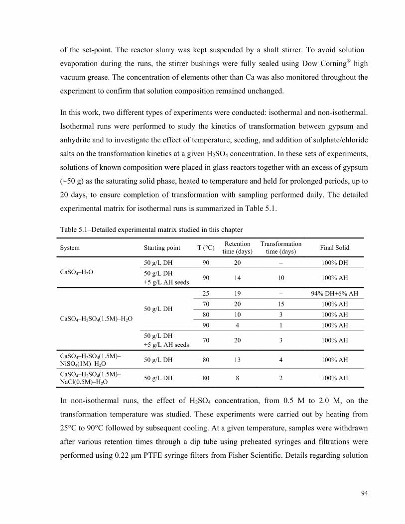
94

of the set-point. The reactor slurry was kept suspended by a shaft stirrer. To avoid solution

evaporation during the runs, the stirrer bushings were fully sealed using Dow Corning® high

vacuum grease. The concentration of elements other than Ca was also monitored throughout the

experiment to confirm that solution composition remained unchanged.

In this work, two different types of experiments were conducted: isothermal and non-isothermal.

Isothermal runs were performed to study the kinetics of transformation between gypsum and

anhydrite and to investigate the effect of temperature, seeding, and addition of sulphate/chloride

salts on the transformation kinetics at a given H2SO4 concentration. In these sets of experiments,

solutions of known composition were placed in glass reactors together with an excess of gypsum

(~50 g) as the saturating solid phase, heated to temperature and held for prolonged periods, up to

20 days, to ensure completion of transformation with sampling performed daily. The detailed

experimental matrix for isothermal runs is summarized in Table 5.1.

Table 5.1–Detailed experimental matrix studied in this chapter

System Starting point T (°C) Retention time (days)

Transformation time (days) Final Solid

50 g/L DH 90 20 – 100% DH CaSO4–H2O 50 g/L DH

+5 g/L AH seeds 90 14 10 100% AH

25 19 – 94% DH+6% AH 70 20 15 100% AH 80 10 3 100% AH

50 g/L DH

90 4 1 100% AH CaSO4–H2SO4(1.5M)–H2O

50 g/L DH +5 g/L AH seeds

70 20 3 100% AH

CaSO4–H2SO4(1.5M)– NiSO4(1M)–H2O 50 g/L DH 80 13 4 100% AH

CaSO4–H2SO4(1.5M)– NaCl(0.5M)–H2O 50 g/L DH 80 8 2 100% AH

In non-isothermal runs, the effect of H2SO4 concentration, from 0.5 M to 2.0 M, on the

transformation temperature was studied. These experiments were carried out by heating from

25°C to 90°C followed by subsequent cooling. At a given temperature, samples were withdrawn

after various retention times through a dip tube using preheated syringes and filtrations were

performed using 0.22 μm PTFE syringe filters from Fisher Scientific. Details regarding solution

95

and solid phase compositions at a given temperature along with the retention times for these

sets of experiments are presented in Appendix F (Tables F.2 and F.3).

Withdrawn solution samples were diluted with 5% HNO3 and stored in sealed plastic test tubes

at room temperature. The Ca concentration was determined by ICP–OES analysis using the

317.933 nm emission line. Reproducibility tests showed that the experimentally measured data

are accurate to within ±5%.

Samples of the equilibrating solid phase were also withdrawn, filtered, and washed with a small

amount of denatured alcohol, containing 85% ethanol and 15% methanol, to replace the solution

and dried below 40°C in an oven under vacuum. Powder X-ray diffraction patterns of the solid

samples were collected on a Philips PW3719 diffractometer utilizing Cu Ka radiation in the

range 10–60° 2θ with a step size of 0.02° and a collection time of 1.25 s/step. The generated

patterns were matched against the International Centre for Diffraction Data® files (JCPDF-

ICDD file numbers 070–0982 for gypsum and 072–0916 for anhydrite). The relative amounts of

gypsum and anhydrite present in the solid samples were estimated by the Rietveld refinement

(details are available in Appendix H). In all experiments carried out in this work, gypsum and

anhydrite were the only crystalline species identified. Hemihydrate was not detected in any of

the samples over the temperature range studied (i.e., 25–90°C). The solid samples were also

analyzed by scanning electronic microscopy (SEM) to study the morphology and structural

changes in CaSO4 crystals during the transformation process. SEM images were obtained on a

JEOL JSM-840 scanning electron microscope. Solid sample powders were mounted rigidly on a

specimen holder, called stub, and coated with gold to facilitate charge removal during

microscope operation. To obtain particles cross-section images, solid powders were dropped

into a resin, and then polished. They were also coated with gold to become electrically

conductive. The time between sample withdrawal and XRD/SEM analysis varied from 1 to 10

days. Meanwhile, samples were preserved in a desiccator, protected against moisture and

humidity.

96

5.3 Results and Discussion

5.3.1 Gypsum–Anhydrite Transformation in Water

The stability regions and temperature of transformation between CaSO4 solid phases, i.e.,

gypsum, hemihydrate and anhydrite, have been studied by various researchers (Freyer and

Voigt, 2003; Dutrizac, 2002; Knacke and Gans, 1977; Hardie, 1967; Bock, 1961; Sborgi and

Bianchi, 1940; Posnjak, 1938; Hill, 1937; Van’t Hoff et al., 1903). Figure 5.1 presents the

solubility diagram of CaSO4 in water.

In solubility diagrams, the solid phase with the lowest solubility is the stable phase at a given

temperature. In Figure 5.1, gypsum is the stable phase at low temperatures, whereas, anhydrite

is stable one above 45–50ºC; hemihydrate is metastable at all temperatures. However, it is

experimentally observed that anhydrite does not crystallize from supersaturated solutions in

water with measurable rates at temperatures below ~80–90ºC, even in the presence of anhydrite

seed crystals (Freyer and Voigt, 2003; Dutrizac, 2002).

0 50 100 150 200 250 3000.00

0.01

0.02

0.03

0.04

0.05

0.06

0.07

0.08

CaSO4(s)

CaSO4.2H2O

CaS

O4 so

lubi

lity,

mol

al

Temperature, oC

Gypsum Exp data Anhydrite Exp data Hemihydrate Exp data

CaSO4.0.5H

2O

Figure 5.1 Solubility diagram of CaSO4 in water. Experimental data are from Dutrizac, 2002; Templeton and Rodgers, 1967; Marshall et al., 1964; Sborgi and Bianchi, 1940; Hill and Wills, 1938; Posnjak, 1938; Partridge and White, 1929. Curves obtained from the OLI/MSE model (Azimi et al., 2007).

In the present work, the transformation of gypsum into anhydrite in pure water was studied at

90ºC. In the absence of added anhydrite seeds, gypsum remained stable for periods up to 20

days. In contrast, the addition of 5 g/L (10 wt%) of anhydrite seeds resulted in nearly complete

transformation after 10 days. In these sets of experiments, gypsum and anhydrite were the only

97

crystalline species identified, and no intermediate hemihydrate was detected. Figure 5.2 shows

the percentage of the remaining gypsum in the equilibrating solid phase at various retention

times in water at 90°C obtained from the X-ray diffraction patterns, using Rietveld analysis.

The composition of the equilibrating solid phase is summarized in Appendix F (Table F.1).

0 2 4 6 8 10 12 14 16

0

20

40

60

80

100

Gyp

sum

(%)

Time, days

Starting with 50 g/L gypsum +5 g/L anhydrite seeds

T=90 oC

With no seeding

Figure 5.2 Percentage of gypsum present in the equilibrating solid phase based on XRD results at various retention times for gypsum–anhydrite transformation in water at 90°C.

5.3.2 Theoretical Determination of the Transformation Temperature

Based on the solubility diagram of calcium sulphate in water (Figure 5.1), the gypsum–

anhydrite transformation temperature lies at 45–50°C. However, as presented in the previous

section, the kinetics of the transformation in water is slow such that, in the absence of anhydrite

seeds, gypsum remains practically stable up to ~90°C. It has been found that the addition of

electrolytes, particularly acids, has an accelerating effect on the transformation process (Farrah

et al., 2004; Freyer and Voigt, 2003; Dutrizac, 2002; Nývlt, 1997).

The direct dehydration reaction of gypsum to anhydrite and the appropriate expression of the

equilibrium constant are as follows:

CaSO4•2H2O(s) = CaSO4(s) + 2 H2O(l) (5.1)

2)exp( waRTGK =

Δ−=

o

(5.2)

98

The temperature functionality of ΔG˚ for the gypsum dehydration reaction has been proposed

by Hardie (1967) as follows:

TTTTG log44.710262.057.1792890 2 −++−=Δ o (5.3)

where, ΔG˚ is in cal.mol-1 and T is in K. Substituting ΔG˚ from Eq. (5.3) in Eq. (5.2) provides

the relation between the activity of water (aw) and the transformation temperature, which is

shown in Figure 5.3. Using this figure, the gypsum–anhydrite transformation temperature in

water (aw=1.0) lies at ~45°C, in good agreement with the results obtained from the solubility

diagram (Figure 5.1). For comparison, the equilibrium constant of the gypsum dehydration

reaction (Eq. 5.1) at various temperatures was calculated utilizing the OLI/MSE model. Solving

Eq. (5.2), the activity of water was calculated at various temperatures (also presented in Figure

5.3). Based on the curve obtained from the OLI/MSE model, the transformation temperature in

water is ~40°C, close to the accepted values (Figure 5.1).

Figure 5.3 may be used to obtain the “theoretical” temperature of the gypsum–anhydrite

transformation if the activity of water in the solution is known. However, it should be noted that,

in most cases, the kinetics of the transformation near theoretical temperatures are slow, resulting

in gypsum retention as a metastable phase for greater periods of time.

0.4 0.5 0.6 0.7 0.8 0.9 1.00

10

20

30

40

50

60

70

80

MSE model

T/ o C

awater

CaSO4.2H

2O

(s)=CaSO

4(s)+2H

2O

(l)

Hardie (1967)

Figure 5.3 Theoretical transformation temperature of gypsum into anhydrite as a function of the activity of water. Solid curve derived from Hardie (1967); dashed curve obtained from the OLI/MSE model.

99

5.3.3 Effect of Sulphuric Acid on the Gypsum Transformation

A few theoretical studies have been undertaken to determine the effect of H2SO4 addition on the

gypsum transformation (Ling and Demopoulos, 2004; Freyer and Voigt, 2003; Raju and

Atkinson, 1990). The theoretical transformation temperature can be determined using phase

transformation diagrams, Figure 5.3, if the activity of water in the solution is known.

In the present work, the effect of acidity on the kinetics of transformation was studied. Slurries

containing ~50 g/L gypsum in 0.5, 1.0, 1.5 and 2.0 M H2SO4–H2O solutions were heated from

25°C to 90°C, and subsequently cooled to 25°C. Slurries were held for various retention times

between 48 h and 72 h at a given temperature, and samples were taken on a daily basis. No

anhydrite seed was added in these runs.

Figures 5.4 (a) to (d) show the concentrations of CaSO4 at different temperatures for various

retention times. In all cases, the solubility of CaSO4 first increases with increasing temperature

up to 70–90°C, depending on the acid concentration, then drops. X-ray diffraction analysis of

the saturating solid phases shows that, in all cases, gypsum began to transform slowly to

anhydrite. Nevertheless, all solids contained less than 20% anhydrite below ~70°C. At

temperatures above 70°C, however, the transformation of gypsum into anhydrite progressed

significantly. In 0.5 M H2SO4 solutions, complete transformation was obtained at 90°C after 4

days (96 h), whereas in 1.0 M acid, 3 days (72 h) was sufficient at the same temperature (90°C).

In solutions containing 1.5 M and 2.0 M H2SO4, complete transformation was achieved at 80°C

after 3 days and 1 day, respectively. The corresponding solubility data and the composition of

the saturating solids at a given temperature at various retention times are summarized in

Appendix F (Tables F.2, F.3).

Results indicate that gypsum is kinetically stable to at least 80°C for acid concentrations as high

as 2.0 M, confirming the results of other studies (Dutrizac, 2002). During cooling, anhydrite was

detected as the only solid phase above 45°C, but further cooling resulted in the conversion of

anhydrite to gypsum. Higher acid concentrations retain more anhydrite after slurries were

cooled to room temperature.

The implication here is that the conversion of gypsum to less soluble anhydrite would occur

rapidly in many industrial processes containing modest concentrations of sulphuric acid (above

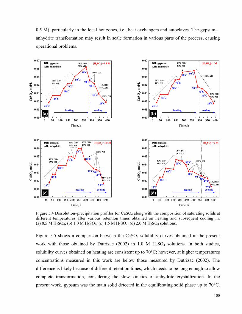
100

0.5 M), particularly in the local hot zones, i.e., heat exchangers and autoclaves. The gypsum–

anhydrite transformation may result in scale formation in various parts of the process, causing

operational problems.

0 50 100 150 200 250 300 350 4000.00

0.01

0.02

0.03

0.04

0.05

0.06

0.07

100% DH

15% DH+85% AH

25% DH+75% AH

100% AH

95% DH+5% AH

cooling

25oC

45oC

70oC90oC

90oC

80oC

70oC

60oC

45oC

25oC

CaS

O4, m

ol/L

Time, h

heating

DH: gypsumAH: anhydrite

[H2SO4]=0.5 M

(a)0 50 100 150 200 250 300 350 400

0.00

0.01

0.02

0.03

0.04

0.05

0.06

0.07

(b)

[H2SO4]=1 M

30% DH+70% AH

80% DH+20% AH

100% AH

90% DH+10% AH

cooling

25oC

45oC70oC

90oC

90oC80oC

70oC

60oC

45oC

25oC

CaS

O4, m

ol/L

Time, h

heating

DH: gypsumAH: anhydrite

0 50 100 150 200 250 300 350 400 4500.00

0.01

0.02

0.03

0.04

0.05

0.06

0.07

(c)

15% DH+85% AH

60% DH+40% AH

80oC85% DH+15% AH

[H2SO4]=1.5 M80% DH+20% AH

100% AH

cooling25oC

45oC70oC90oC

80oC

70oC

60oC

45oC

25oC

CaS

O4, m

ol/L

Time, h

heating

DH: gypsumAH: anhydrite

0 50 100 150 200 250 300 350 400 4500.00

0.01

0.02

0.03

0.04

0.05

0.06

0.07

(d)

5% DH+95% AH

80oC

82% DH+18% AH

[H2SO4]=2 M

70% DH+30% AH

100% AH

cooling25oC

45oC70oC

90oC

80oC70oC

60oC

45oC

25oC

C

aSO

4, mol

/L

Time, h

heating

DH: gypsumAH: anhydrite

Figure 5.4 Dissolution–precipitation profiles for CaSO4 along with the composition of saturating solids at different temperatures after various retention times obtained on heating and subsequent cooling in: (a) 0.5 M H2SO4; (b) 1.0 M H2SO4; (c) 1.5 M H2SO4; (d) 2.0 M H2SO4 solutions.

Figure 5.5 shows a comparison between the CaSO4 solubility curves obtained in the present

work with those obtained by Dutrizac (2002) in 1.0 M H2SO4 solutions. In both studies,

solubility curves obtained on heating are consistent up to 70°C; however, at higher temperatures

concentrations measured in this work are below those measured by Dutrizac (2002). The

difference is likely because of different retention times, which needs to be long enough to allow

complete transformation, considering the slow kinetics of anhydrite crystallization. In the

present work, gypsum was the main solid detected in the equilibrating solid phase up to 70°C.

101

At 80°C, the transformation reaction moved forward and complete transformation was

obtained at 90°C after 3 days (72 h). In the experiment performed by Dutrizac (2002), gypsum

was detected as the main solid phase up to 90°C with ~24 h retention time and transformation

completed at 95°C.

20 30 40 50 60 70 80 90 1000.00

0.01

0.02

0.03

0.04

0.05

0.06

0.07

0.08

30% DH+70% AH

100% AH

100% AH

100% AH80% DH+20% AH

CaS

O4, m

ol/L

Temperature, oC

This work, heating This work, cooling Dutrizac (2002), heating Dutrizac (2002), cooling

[H2SO4]=1 M

Figure 5.5 Concentration of CaSO4 in 1.0 M H2SO4 solutions as a function of temperature: (▲) this work, heating; (∆) this work, cooling; (■) Dutrizac (2002), heating; (□) Dutrizac (2002), cooling.

5.3.4 Theoretical and Practical Stability Regions of Gypsum in H2SO4 Solutions

The kinetics of gypsum–anhydrite transformation is an important factor to be considered in the

solubility determination of systems containing calcium sulphate hydrates. To demonstrate the

significance of such considerations, the “theoretical” and “practical” stability regions of gypsum

and anhydrite are marked in Figure 5.6. The solid curve represents the theoretical transition of

gypsum into anhydrite in H2SO4–H2O solutions obtained from the OLI/MSE model utilizing the

recently developed database (Azimi et al., 2007, 2008). The phase diagram in Figure 5.6 was

constructed using a procedure similar to that suggested by Li and Demopoulos (2006c).

Based on the results obtained in the present work, gypsum was kinetically stable up to 80°C

within the indicated acid range. The exact transformation temperature at a given acid

concentration along with the observed retention times are also presented in Figure 5.6. Region

(II), the area between the equilibrium transition curve and an upper line, is the practical stability

region of gypsum (based on retention time of 1–3 days). That is, in this region, the degree of

metastability of gypsum is significant and an induction period is required to complete the

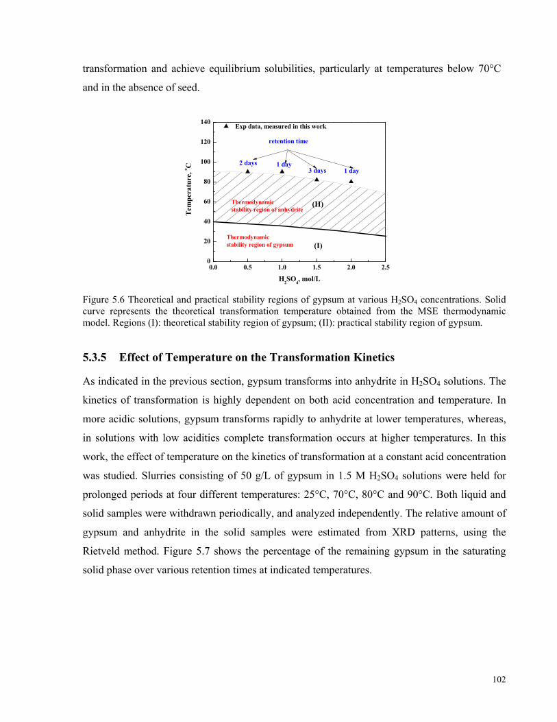
102

transformation and achieve equilibrium solubilities, particularly at temperatures below 70°C

and in the absence of seed.

0.0 0.5 1.0 1.5 2.0 2.50

20

40

60

80

100

120

140

(II)

Exp data, measured in this work

Thermodynamicstability region of anhydrite

1 day3 days1 day2 days

Tem

pera

ture

, o C

H2SO4, mol/L

Thermodynamicstability region of gypsum

retention time

(I)

Figure 5.6 Theoretical and practical stability regions of gypsum at various H2SO4 concentrations. Solid curve represents the theoretical transformation temperature obtained from the MSE thermodynamic model. Regions (I): theoretical stability region of gypsum; (II): practical stability region of gypsum.

5.3.5 Effect of Temperature on the Transformation Kinetics

As indicated in the previous section, gypsum transforms into anhydrite in H2SO4 solutions. The

kinetics of transformation is highly dependent on both acid concentration and temperature. In

more acidic solutions, gypsum transforms rapidly to anhydrite at lower temperatures, whereas,

in solutions with low acidities complete transformation occurs at higher temperatures. In this

work, the effect of temperature on the kinetics of transformation at a constant acid concentration

was studied. Slurries consisting of 50 g/L of gypsum in 1.5 M H2SO4 solutions were held for

prolonged periods at four different temperatures: 25°C, 70°C, 80°C and 90°C. Both liquid and

solid samples were withdrawn periodically, and analyzed independently. The relative amount of

gypsum and anhydrite in the solid samples were estimated from XRD patterns, using the

Rietveld method. Figure 5.7 shows the percentage of the remaining gypsum in the saturating

solid phase over various retention times at indicated temperatures.

103

0 2 4 6 8 10 12 14 16 18 20

0

20

40

60

80

100

Gyp

sum

(%)

Time, days

25 oC 70 oC 80 oC 90 oC

1.5 M H2SO4, 50 g/L gypsum, no anhydrite seeding

Figure 5.7 Kinetics of gypsum–anhydrite transformation at various temperatures in 1.5 M H2SO4 solutions in the absence of anhydrite seeds.

At 25°C, gypsum remained nearly unchanged, with about 5–10% transformation into anhydrite,

for up to 19 days. The XRD patterns of the solid samples withdrawn after 9 h, 24 h and 19 days

are presented in Appendix D. In addition, SEM images of these solid samples are presented in

Appendix G (Figure G.1). At 70°C, gypsum remained the dominant solid phase, with about 10%

anhydrite present, for 8 days, then the transformation accelerated and completed after 15 days of

contact. In runs at 80°C and 90°C, complete transformation occurred after 3 days and 1 day,

respectively. In these experiments, the induction period strongly depended on temperature.

In these sets of experiments, X-ray diffraction analysis of the solid samples indicated an initial

transformation of gypsum into anhydrite in the first few hours. This observation is in contrast

with the results reported by Dutrizac and Kuiper (2008), where gypsum remained unchanged

over a period of time before transforming to stable anhydrite. However, initial transformation

was observed by other researchers. Hardie (1967) has mentioned that in a few of the runs in

which anhydrite was produced from gypsum, a rind, presumed from X-ray diffraction to be

anhydrite, was observed on the surface and along cleavage cracks of gypsum crystals. In his

experiments, about 10–15% of the gypsum grains showed such alterations. Based on these

observations, Hardie (1967) suggested that gypsum directly dehydrates to anhydrite, beginning

at the crystal surfaces where H2O may be transferred to the solution phase.

The discrepancy with Dutrizac and Kuiper’s data is likely due to the solid samples handling. In

all experiments carried out in this work, solids were washed by a small amount of denatured

104

alcohol to replaces the solution, and dried inside an oven at 35–40°C. In the experiments

performed by Dutrizac and Kuiper (2008), solid samples were first washed with a small amount

of water and then with alcohol, and they were air-dried at room temperature. The addition of

water to the solid samples and drying at room temperature, where gypsum is the stable phase,

may have resulted in rehydration of anhydrite formed on the surface of gypsum crystals. The

phenomenon of initial transformation is explained in detail in Section 5.3.8.

The crystallization of stable anhydrite after initial transformation has been found to be surface

controlled, following a rate equation second-order in supersaturation (Nancollas, 1979):

2)( sc cckdtdc

−= (5.4)

where dc/dt is the linear rate of the reaction, kc is the rate constant of anhydrite crystallization,

and (c–cs) is the absolute super-saturation. By considering the fact that the rate constant of

anhydrite crystallization (kc) is inversely proportional to the induction time, i.e., kc=τ/tind, where

τ is a constant in mol-1, and substituting kc in the Arrhenius equation, the following empirical

relation is obtained (Turenne et al., 1999; Liu and Nancollas, 1975):

)exp(1RTEA

ta

ind

−=τ

(5.5)

where tind is the induction time, A is the Arrhenius (pre-exponential) constant, Ea is the

activation energy, R is the gas constant and T is absolute temperature. Equation (5.5) can be

used to calculate the activation energy associated with the induction time for the crystallization

of stable anhydrite. The ln(tin) vs. 1/T is plotted in Figure 5.8 which shows a linear relationship

(R2=0.99). The corresponding apparent activation energy, calculated from the slope of the

straight line, is 35 kcal•mol-1. As expected, this value is higher than that calculated by Liu and

Nancollas (1970, 1975) for gypsum (15 kcal•mol-1).

105

2.75 2.80 2.85 2.90 2.950.00.51.01.52.02.53.03.54.04.55.05.56.06.57.0

T=70 oC

T=80 oC

ln (t

ind)

1000/T (K-1)

Y=17.61 X - 46.29T=90 oC

[H2SO

4]=1.5 M

R2=0.99

Figure 5.8 Variation of the ln(tin) vs. 1/T at various temperatures in 1.5 M H2SO4 solutions with no seeds present.

5.3.6 Effect of Seeding on Gypsum–Anhydrite Transformation

Effect of seeding on the kinetics of the transformation has been studied previously (Dutrizac and

Kuiper, 2008, 2006; Farrah et al., 2004) which indicated the significant role of seeding in the

transformation process. In the present work, the effect of seeding on the gypsum–anhydrite

transformation was also studied in 1.5 M H2SO4 solutions at 70°C. Slurries were prepared by

adding 50 g/L of gypsum, together with 5 g/L of anhydrite seeds into the solutions. Slurries

were periodically sampled, and both the liquid and solid samples were analyzed independently.

Figure 5.9 shows the percentage of the remaining gypsum in the solid samples at various

retention times in the presence of anhydrite seeds compared with that where no seed was added.

As is shown, the addition of 5 g anhydrite seeds to the system containing 50 g of gypsum in

1.5M H2SO4 results in a significantly more rapid transformation of gypsum into anhydrite. In

the absence of anhydrite seeds, complete transformation occurred after 15 days, whereas with

seeding, 2 days was sufficient for near complete transformation.

106

0 2 4 6 8 10 12 14 16 18 20

0

20

40

60

80

100

Gyp

sum

(%)

Time, days

50 g/L gypsum in1.5 M H

2SO

4 solutions

T=70 oC

No seeding

With 5 g/Lanhydrite seeds

Figure 5.9 Kinetics of gypsum–anhydrite transformation at 70°C in 1.5 M H2SO4 solutions in the presence of an initial 5 g/L of anhydrite seeds compared to no seeding case.

Figure 5.10 presents a comparison between the CaSO4 concentration at different retention times

in 1.5 M H2SO4 slurries in the presence of 5 g/L anhydrite seeds compared to no seeding. The

dashed lines represent the saturation levels of gypsum and anhydrite in the system. The

difference between the time for transforming gypsum into anhydrite and for discharging the

supersaturation in the presence of seed can be explained by the slow crystallization kinetics of

anhydrite (Freyer and Voigt, 2003; Nancollas et al., 1973). Similar discrepancy between solid

and solution phase data has been observed by other researchers (Farrah et al., 2004). This

observation indicates that the transformation involves a dissolution–precipitation mechanism.

The end result here is that seeding accelerates the kinetics of the transformation. Therefore,

process solutions saturated with gypsum at temperatures between 60–70°C would reject their

calcium content faster in the presence of anhydrite seeds, which would result in lowering the

risk of anhydrite scale formation inside autoclaves or other hot zones throughout the plant. This

is in contrast to the current industrial practice where gypsum seed is recycled instead.

107

0 2 4 6 8 10 12 14 16 18 200.00

0.01

0.02

0.03

0.04

0.05

0.06

0.07

Anhydrite saturation line

CaS

O4 c

once

ntra

tion,

mol

/L

Time, days

No seeding 5 g/L anhydrite seed

50 g/L gypsum in 1.5M H2SO4 solutions

T=70 oC

Gypsum saturation line

Figure 5.10 CaSO4 solubility in 1.5 M H2SO4 solutions at 70°C at various residence times in the presence of 5 g/L anhydrite seeds compared to no seeding case.

5.3.7 Effect of Sulphate and Chloride Salts on the Transformation Process

As indicated in the previous sections, H2SO4 increases the rate of gypsum–anhydrite

transformation. Since many industrial processes contain other electrolytes than acid, the effect

of adding NiSO4 and NaCl on the transformation process was also studied in this work. To

assess the transformation process, slurries consisting of 50 g/L gypsum in 1.0 M NiSO4–1.5 M

H2SO4 and 0.5 M NaCl–1.5 M H2SO4 solutions were held for prolonged periods (up to 14 days).

Results obtained show that the addition of 1.0 M NiSO4 into 1.5 M H2SO4 solution slows the

kinetics of the transformation. In the absence of NiSO4, complete transformation was achieved

within 4 days, whereas, in the presence of 1.0 M NiSO4, one additional day was required. In

contrast, the addition of 0.5 M NaCl results in faster transformation kinetics (completed within 2

days). Figure 5.11 presents the percentage of the remaining gypsum in the saturating solid phase

at various retention times in the systems studied, compared to those in H2SO4 only solutions.

108

0 2 4 6 8 10 12 14

0

20

40

60

80

100

Time, days

T=80 oC

Gyp

sum

(%)

1.5 M H2SO4-1 M NiSO4

1.5 M H2SO4

1.5 M H2SO4-0.5 M NaCl

Figure 5.11 Kinetics of gypsum–anhydrite transformation at 80°C in: (–■–) acid only (1.5 M H2SO4);(–▲–) 1.0 M NiSO4–1.5 M H2SO4; (– –) 0.5 M NaCl–1.5 M H2SO4 solutions.

Figure 5.12 shows the respective concentrations of calcium sulphate. Addition of 1.0 M NiSO4

to a 1.5 M H2SO4 solution decreases the solubility of calcium sulphate by about 60% due to the

common ion effect of added SO42- ions, whereas, the addition of 0.5 M NaCl slightly increases

the solubility (by ~7%). In this figure, the dashed lines represent the saturation levels of gypsum

and anhydrite in the solutions.

0 2 4 6 8 10 12 140.00

0.02

0.04

0.06

0.08

0.10T=80 oC

Anhydrite saturation

Gypsum saturation

Anhydrite saturation

CaS

O4 c

once

ntra

tion,

mol

/L

Time, days

1.5 M H2SO4

1 M NiSO4-1.5 M H2SO4

0.5 M NaCl-1.5 M H2SO

4

Gypsum saturation

Figure 5.12 Calcium sulphate concentrations vs. retention time at 80°C: (–■–) in acid only (1.5 M H2SO4); (–▲–) in 1.0 M NiSO4–1.5 M H2SO4; (– –) in 0.5 M NaCl–1.5 M H2SO4 solutions.

The transformation kinetics depends on both dissolution kinetics of gypsum as well as

nucleation and growth of anhydrite (Freyer and Voigt, 2003; Kontrec et al.; 2002). Figure 5.13

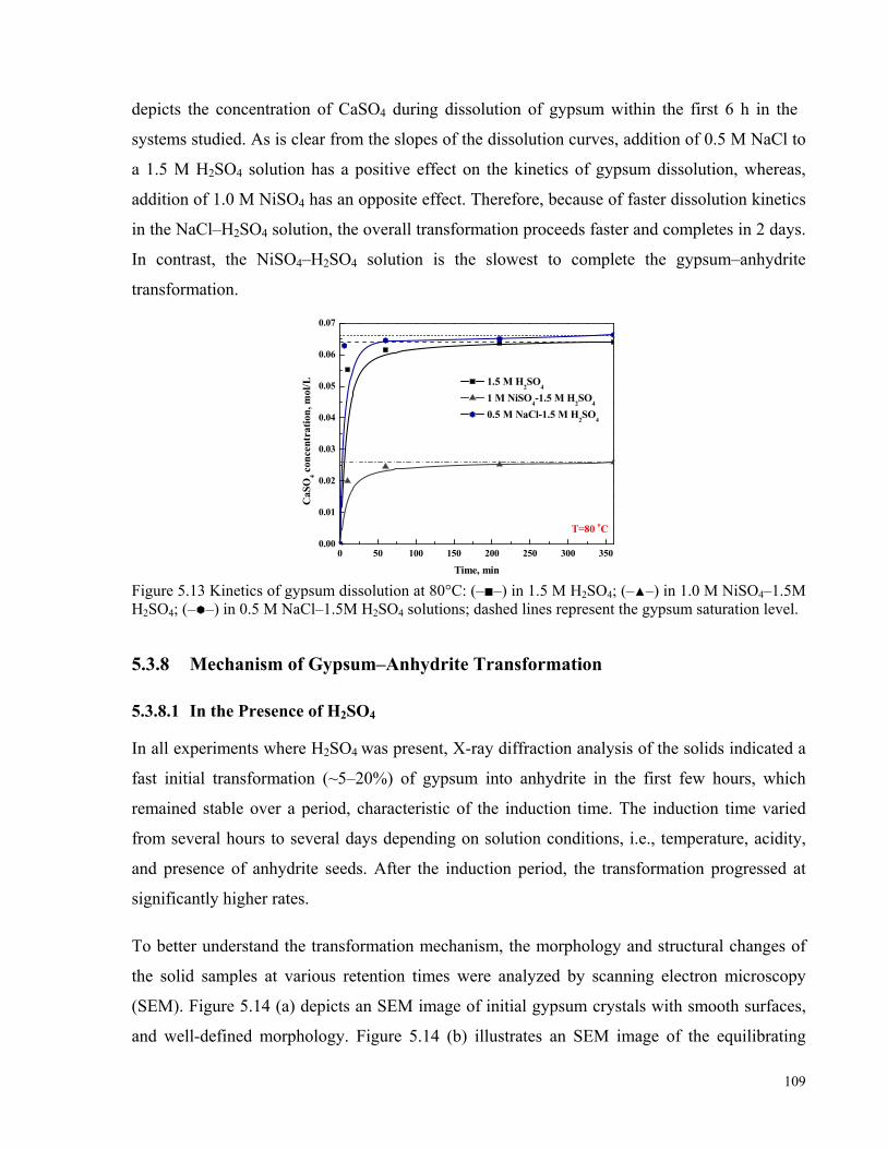
109

depicts the concentration of CaSO4 during dissolution of gypsum within the first 6 h in the

systems studied. As is clear from the slopes of the dissolution curves, addition of 0.5 M NaCl to

a 1.5 M H2SO4 solution has a positive effect on the kinetics of gypsum dissolution, whereas,

addition of 1.0 M NiSO4 has an opposite effect. Therefore, because of faster dissolution kinetics

in the NaCl–H2SO4 solution, the overall transformation proceeds faster and completes in 2 days.

In contrast, the NiSO4–H2SO4 solution is the slowest to complete the gypsum–anhydrite

transformation.

0 50 100 150 200 250 300 3500.00

0.01

0.02

0.03

0.04

0.05

0.06

0.07

CaS

O4 c

once

ntra

tion,

mol

/L

Time, min

1.5 M H2SO

4

1 M NiSO4-1.5 M H2SO4

0.5 M NaCl-1.5 M H2SO4

T=80 oC

Figure 5.13 Kinetics of gypsum dissolution at 80°C: (–■–) in 1.5 M H2SO4; (–▲–) in 1.0 M NiSO4–1.5M H2SO4; (– –) in 0.5 M NaCl–1.5M H2SO4 solutions; dashed lines represent the gypsum saturation level.

5.3.8 Mechanism of Gypsum–Anhydrite Transformation

5.3.8.1 In the Presence of H2SO4

In all experiments where H2SO4 was present, X-ray diffraction analysis of the solids indicated a

fast initial transformation (~5–20%) of gypsum into anhydrite in the first few hours, which

remained stable over a period, characteristic of the induction time. The induction time varied

from several hours to several days depending on solution conditions, i.e., temperature, acidity,

and presence of anhydrite seeds. After the induction period, the transformation progressed at

significantly higher rates.

To better understand the transformation mechanism, the morphology and structural changes of

the solid samples at various retention times were analyzed by scanning electron microscopy

(SEM). Figure 5.14 (a) depicts an SEM image of initial gypsum crystals with smooth surfaces,

and well-defined morphology. Figure 5.14 (b) illustrates an SEM image of the equilibrating

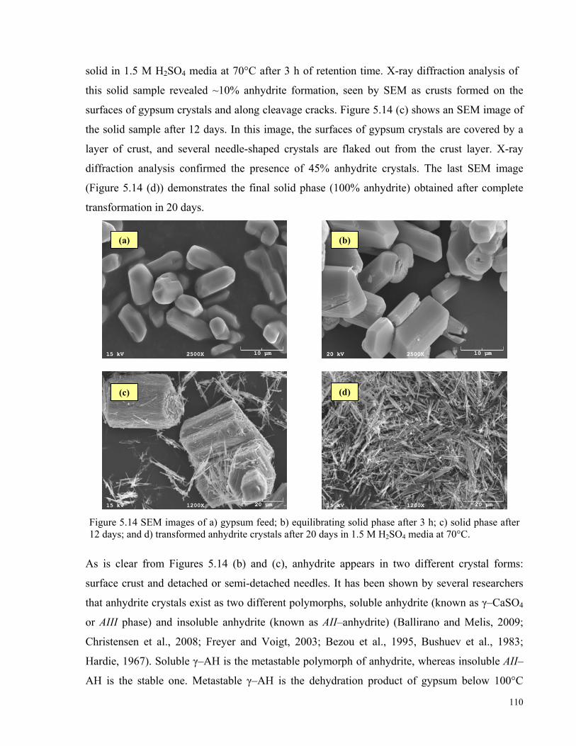
110

solid in 1.5 M H2SO4 media at 70°C after 3 h of retention time. X-ray diffraction analysis of

this solid sample revealed ~10% anhydrite formation, seen by SEM as crusts formed on the

surfaces of gypsum crystals and along cleavage cracks. Figure 5.14 (c) shows an SEM image of

the solid sample after 12 days. In this image, the surfaces of gypsum crystals are covered by a

layer of crust, and several needle-shaped crystals are flaked out from the crust layer. X-ray

diffraction analysis confirmed the presence of 45% anhydrite crystals. The last SEM image

(Figure 5.14 (d)) demonstrates the final solid phase (100% anhydrite) obtained after complete

transformation in 20 days.

Figure 5.14 SEM images of a) gypsum feed; b) equilibrating solid phase after 3 h; c) solid phase after 12 days; and d) transformed anhydrite crystals after 20 days in 1.5 M H2SO4 media at 70°C.

As is clear from Figures 5.14 (b) and (c), anhydrite appears in two different crystal forms:

surface crust and detached or semi-detached needles. It has been shown by several researchers

that anhydrite crystals exist as two different polymorphs, soluble anhydrite (known as γ–CaSO4

or AIII phase) and insoluble anhydrite (known as AII–anhydrite) (Ballirano and Melis, 2009;

Christensen et al., 2008; Freyer and Voigt, 2003; Bezou et al., 1995, Bushuev et al., 1983;

Hardie, 1967). Soluble γ–AH is the metastable polymorph of anhydrite, whereas insoluble AII–

AH is the stable one. Metastable γ–AH is the dehydration product of gypsum below 100°C

(a) (b)

(c) (d)

111

(where hemihydrate formation does not occur), or that of hemihydrate at temperatures above

100°C. It has been reported that the crystallization of the stable AII–AH is the slowest compared

to other calcium sulphate phases, and requires a long induction period (Christensen et al., 2008;

Farrah et al., 2004; Freyer and Voigt, 2003; Nancollas et al., 1973). Freyer and Voigt (2003)

concluded that in aqueous solutions, the transformation of gypsum into stable AII–AH is not a

direct reaction.

There are very few published proven structural differences between γ–AH and AII–AH, which

often lead to terminological confusion (Bushuev et al., 1983). In addition, the hydration rate of

γ–AH has been reported to be high (Christensen et al., 2008; Bushuev et al., 1983); therefore,

fast re-hydration of γ–AH may prevent this polymorph from being indentified if samples have

been in contact with water at room temperature prior to XRD/SEM analysis. The situation is

more complicated by the fact that the X-ray diffraction patterns of γ–AH and AII–AH are very

similar (Bushuev et al., 1983) and they can be distinguished only by using high-resolution X-ray

diffractometers. Figure 5.15 shows the XRD patterns for the two anhydrite polymorphs obtained

from International Centre for Diffraction Data® files (JCPDF-ICDD file number 072–0916 for

orthorhombic AII–anhydrite and 037–0184 for tetragonal γ–anhydrite).

Figure 5.15 XRD patterns of AII–anhydrite: 072-0916 (orthorhombic) and γ–anhydrite: 037-0184 (tetragonal) obtained from ICDD database. The characteristic line of AII–AH is marked with an asterisk.

As is clear, the patterns of the two anhydrite polymorphs (soluble and insoluble) are very

similar, except for a characteristic peak distinguishing these two patterns, located at 2θ=41.3°,

* AII–AH (stable)

γ–AH (metastable)

112

which is marked by an asterisk in Figure 5.15. Therefore, below 45°, the XRD patterns for both

anhydrites overlap.

The X-ray diffraction patterns of the intermediate solid samples presented in Figures 5.14 (b)

and (c), collected in the range of 10–55° 2θ, are presented in Appendix D (Figures D.5 and D.6).

The characteristic peak of the stable AII–AH was not detected in the solid sample withdrawn

after 3 h of retention, whereas, it was detected in the solid sample taken after 12 days, where

needle-shaped crystals were also present. Based on these observations, it is likely that the

product of initial dehydration of gypsum is the soluble γ–AH polymorph. However, further

investigations are required to claim this phenomenon without any doubt.

As presented in the previous sections, addition of anhydrite (AII–AH) seeds, both in pure water

and in H2SO4 solutions, shortens the induction time and accelerates the transformation process,

which is evident that the transformation involves a dissolution–precipitation step.

Moreover, no hemihydrate formation was detected in the solid samples analyzed after various

retention times, over the entire temperature and acid concentration ranges studied (i.e., 25–90°C,

and 0–2.0 M H2SO4). Similar behaviour has been observed by others in H2SO4 media at

temperatures below 100°C (Dutrizac and Kuiper, 2008; Farrah et al., 2004; Hardie, 1967).

Based on the above observations, the following mechanism is postulated for the gypsum–

anhydrite transformation in acidic solutions (0.5–2 M H2SO4), over the temperature range of

25–90°C:

(i) Gypsum quickly dehydrates to soluble γ–AH at the crystal–solution interface, along

cleavage cracks, where H2O can be transferred to the aqueous phase (a similar

phenomenon was also assumed to take place by Hardie (1967)). Since the initial

surface dehydration was only observed in the experiments carried out in the presence

of H2SO4 (not in pure water), the reason for that can be attributed to the presence of

H+ ions (from H2SO4), which facilitate stripping out water molecules from the

surface of gypsum crystals, by surface complexation and external H3O+ formation.

(ii) Then, nuclei of stable AII–AH form, likely as a result of polymorphic transition

between γ–AH and AII–AH. If the nucleation of AII–AH occurs on the γ–AH

surface, two possible mechanisms can be envisaged for the formation of AII–AH

113

nuclei, as proposed by Petit and Conquerel (1996). The first mechanism involves

cooperative molecular movements which result in a local deformation of the

structure from the parent phase to the daughter phase. The second possible

mechanism consists of breaking the intermolecular links, followed by a repositioning

of each molecule. Nevertheless, the exact nucleation mechanism of these

polymorphic transitions at molecular level cannot be fully elucidated from the

available experimental data.

(iii) After nucleation of stable AII–AH, the growth of AII–AH nuclei occurs. At first, the

bulk of the solution rejects its super-saturation on the newly-formed stable AII–AH

nuclei. Since the stable AII–AH forms needle-like crystals, resulting in a highly

porous coating, it allows further dissolution of gypsum particles sustaining a super-

saturated solution with respect to AII–AH, and therefore precipitating on and

growing the AII–AH nuclei present on their exterior surface. As the dissolution

proceeds, the interface between the undissolved gypsum (the core) and the outer

layer consisting of AII–AH crystals recedes towards the centre of the gypsum particle

in a fashion similar to the shrinking core model (Hsu et al., 2009; Wen, 1968).

A series of SEM images obtained at various retention times are presented in Figure 5.16 (a)–(e)

to depict the transformation mechanism in 1.5 M H2SO4 solutions at 80°C. In these images, both

particles and cross-sections are presented. Figure 5.16 (a) presents an SEM image of gypsum

feed crystals. Figures 5.16 (b) shows solid samples after 24 h retention, where an exterior layer

of anhydrite appears around the gypsum core on the cross-section image. The SEM images of

solid samples after 34 h and 56 h, are presented in Figures 5.16 (c) and (d), respectively. A

comparison between Figures (b), (c) and (d) reveals that the interface between the undissolved

gypsum and the exterior anhydrite layer moves inward (i.e., gypsum core shrinks) with time. It

also appears that the AII–AH coating starts to disintegrate partially after ~56 h. Figure 5.16 (e)

depicts the final needle-shaped anhydrite particles produced after 80 h.

114

(a) t=0 h 100% DH

(b) t=24 h 85% DH+15% AH

(c) t=34 h 58% DH+42% AH

(d) t=56 h 35% DH+65% AH

(e) t=80 h 100% AH

Figure 5.16 SEM images of saturating solids in 1.5 M H2SO4 media at 80°C after various retention times.

115

5.3.8.2 Transformation Mechanism in Pure Water

Contrary to gypsum behaviour in H2SO4 solutions, gypsum in pure water remained unchanged

(tested for 20 days) at temperatures as high as 90°C in the absence of anhydrite seeds, whereas

addition of 10wt% anhydrite seeds (AII–AH) accelerated the transformation. In these

experiments, the initial dehydration of gypsum to γ–AH was not detected by XRD; therefore,

the transformation is likely to proceed directly through gypsum dissolution followed by AII–AH

precipitation. Several SEM images related to the experiments performed in water are presented

in Appendix G, providing further support to the above conclusions.

More powerful and precise techniques with high resolution detectability such as in situ

synchrotron radiation powder X-ray diffraction (SR-PXD) are required to study the

transformation mechanism rigorously at the atomic level. Utilizing such techniques allows

following all changes in the morphologies and characteristics of the solids in situ over very short

exposure times. In the present work, however, the transformation between gypsum and

anhydrite was investigated at the macroscopic level, with a focus on the effect of various

parameters on the transformation kinetics, to understand the effect of gypsum–anhydrite

transformation on the calcium sulphate scaling problem in the industry. Therefore, the

mechanism proposed is based only on XRD patterns and SEM images of the equilibrating solids

at various retention times, and cannot account for all the changes taking place at the atomic

scale.

5.3.9 Industrial Implication: Precipitation due to Super-saturation

It was shown in the previous sections that in the absence of seeds, gypsum transforms into

insoluble anhydrite in 1.5 M H2SO4 solutions at 80°C after 3 days through gypsum dissolution

followed by nucleation and growth of anhydrite. It is of great practical importance to further

investigate the extent of this transformation in the presence of seed crystals, because it may offer

an opportunity to reduce calcium super-saturation to anhydrite saturation level, which is lower

than that of gypsum, enabling more efficient process water utilization. To this end, a solution of

1.5 M H2SO4 saturated with gypsum at 80°C was prepared. The solution was kept at

temperature for 24 h before 10 g of anhydrite seeds were added. Both liquid and solid samples

were withdrawn periodically and analyzed independently. Figure 5.17 shows the concentration

of CaSO4 as a function of residence time. The first sample was withdrawn before adding

116

anhydrite seeds and represents the saturation level of gypsum. After adding 10 g/L of anhydrite

seeds to the system, the CaSO4 concentration dropped sharply within the first few hours and

after 1 day it almost reached the saturation level of anhydrite in the solution. X-ray diffraction

analysis of the solid samples withdrawn at various retention times detected only anhydrite.

0 20 40 60 80 100 120 140 1600.02

0.03

0.04

0.05

0.06

0.07

0.08

Anhydrite saturation level

CaS

O4, m

ol/L

time, h

Gypsum saturation level

[H2SO

4]=1.5 M

T=80 oC

10 g of anhydrite seed

Figure 5.17 CaSO4 concentration at various retention times in 1.5 M H2SO4 solutions initially saturated with gypsum at 80°C after adding 10 g of anhydrite seeds.

The implication of this study is that process solutions saturated with gypsum at moderate

temperatures (above ~80°C) can be seeded with anhydrite to decrease their calcium content and

lower it to the saturation level of anhydrite, provided that the solution is slightly acidic (~0.5 M

H2SO4). This would result in decreasing the risk of scale formation downstream.

117

5.4 Summary

The kinetics of the gypsum–anhydrite transformation was investigated by monitoring changes in

both liquid and solid phases. The results showed that in pure water, gypsum remained stable up

to 90°C in the absence of anhydrite seeds for a prolonged time (tested for up to 20 days). The

addition of 10 wt% anhydrite seeds accelerated the transformation process in water at similar

temperature (90ºC), resulting in complete transformation after 10 days.

The addition of 0.5 M to 2.0 M H2SO4 was found to promote the transformation process. In

0.5 M H2SO4 solutions, complete transformation was achieved at 90°C after 4 days (96 h),

whereas in 1.0 M acid, 3 days (72 h) was sufficient at the same temperature (90°C). In solutions

containing 1.5 M and 2.0 M H2SO4, complete transformation occurred at 80°C after 3 days and

1 day, respectively. Therefore, gypsum is kinetically stable up to at least 80°C for acid

concentrations as high as 2.0 M. In experiments performed in H2SO4 solutions, anhydrite was

detected as the equilibrating solid phase during cooling process above 45°C, but further cooling

resulted in the conversion of anhydrite to gypsum. Higher acid concentrations made solutions

retain more anhydrite after slurry was cooled to room temperature.

Temperature was shown to have a significant effect on the transformation kinetics. In 1.5 M

H2SO4 solutions, gypsum remained almost unchanged at 25°C over the period tested (i.e., 18

days); at 70°C, gypsum remained the dominant solid phase for 7 or 8 days with less than 10% γ–

anhydrite present; after 8 days, the transformation progressed more rapidly and completed after

15 days of contact. In the runs at 80°C and 90°C, complete transformation occurred after 3 days

and 1 day, respectively. By using induction times at these temperatures and fitting of the

Arrhenius expression, the apparent activation energy for the crystallization of stable AII–

anhydrite was calculated to be 35 kcal•mol-1.

The addition 1.0 M NiSO4 to a 1.5 M H2SO4 solution at 80°C had an impending effect on the

transformation process by causing a 1 day delay. In contrast, the addition of 0.5 M NaCl as a

representative chloride salt to a 1.5 M H2SO4 solution at the same temperature had a positive

effect and accelerated the transformation process by 1 day. This is due to the fact that the

addition of NiSO4 to 1.5 M H2SO4 solutions has a negative effect on the kinetics of gypsum

118

dissolution due to the common ion effect, whereas the addition of NaCl to 1.5 M H2SO4

solutions has an opposite effect.

In all experiments conducted in this work, an initial transformation (5−20%) of gypsum into

anhydrite (likely to be metastable γ–anhydrite polymorph) was observed in the first few hours

which stayed unchanged over an induction time. The duration of induction periods varied from

several hours to several days depending on temperature, acidity and the presence of seeds. After

the induction period, the transformation progressed at higher rates. Hemihydrate was not

detected in any experiment at 25–90°C. Based on these observations, a mechanism was

proposed for the gypsum–anhydrite transformation in H2SO4 solutions consisting of direct

dehydration of gypsum to metastable γ–anhydrite, followed by the nucleation of stable AII–

anhydrite as a result of polymorphic transitions between γ– and AII–anhydrites. The last stage is

the growth of AII–anhydrite nuclei through a dissolution–precipitation process. As the

dissolution proceeds, the interface between the undissolved gypsum (the core) and the layer

consisting of AII–AH crystals moves inward, following the assumptions of a shrinking core

model.

The implication of the results obtained is that the transformation of gypsum into anhydrite,

which results in a significant drop in the solubility (up to one order of magnitude) would occur

rapidly in many industrial processes with modest concentrations of sulphuric acid (above 0.5 M)

at temperatures above 80°C, particularly in the local hot zones of plants, e.g., autoclaves in

hydrometallurgical processes or heat exchangers in other industries. However, the gypsum–

anhydrite transformation can be utilized for mitigating CaSO4 scaling in various industries. That

is, process solutions saturated with gypsum can be aged in the presence of anhydrite seeds at

moderate temperatures (~80°C) to decrease their calcium content, provided that the solution is

slightly acidic (~0.5 M).

119

CHAPTER 6 CONCLUSIONS

he solution chemistry and phase equilibria of calcium sulphate hydrates (gypsum,

hemihydrate and anhydrite) in multicomponent hydrometallurgical solutions containing

various minerals was investigated over wide ranges of temperature and composition. A new

database for the Mixed Solvent Electrolyte (MSE) model of the OLI software was developed

through fitting of existing literature data such as mean activity, heat capacity and solubility in

simple binary and ternary systems, as well as additional solubility data measured in the present

work. Furthermore, a number of experiments were carried out to investigate the effect of various

parameters including temperature, acidity, as well as metal sulphate and chloride concentrations

on the solubilities of calcium sulphate hydrates in laterite pressure acid leach (PAL) processes,

containing Al2(SO4)3, MgSO4, NiSO4, H2SO4, and NaCl, over the temperature range of

25–250ºC. Prior to this work, no previous study had been conducted for such systems and no

reliable (i.e., experimentally verifiable) chemical models existed.

The database developed, utilized by the MSE model, was shown to accurately predict the

solubilities of all calcium sulphate hydrates (and hence, predict the scaling potential) in various

multicomponent hydrometallurgical process solutions including neutralized zinc sulphate leach

solutions in the Zinc Pressure Oxidation process (Zn-POX), nickel sulphate–chloride solutions

from the Vale Inco Ni-POX process currently under implementation to recover Ni from the

Voisey’s Bay deposit in Newfoundland and Labrador, as well as solutions in the High Pressure

Acid Leach process (HPAL) for Ni and Co recovery from laterite ores over a wide temperature

range of 25–250°C. The fact that modelling in binary and ternary systems is sufficient to predict

the behaviour of more complex multicomponent systems is a substantive contribution to the

existing field. The applicability regions of the model with respect to temperature and

composition are summarized in the following table.

Table 6.1–Applicability regions of the model

Compound Range Compound Range HCl 0–6.0 M H2SO4 0–3.0 M NaCl 0–6.0 M Na2SO4 0–3.6 M LiCl 0–1.0 M MgSO4 0–4.0 M CaCl2 0–5.6 M MnSO4 0–3.7 M MgCl2 0–6.0 M NiSO4 0–3.5 M AlCl3 0–1.5 M ZnSO4 0–2.5 M FeCl3 0–2.2 M Fe2(SO4)3 0–1.0 M Temperature range: 25–250˚C

T

120

The results obtained from the model showed that theoretically gypsum transforms into

anhydrite at around 45–50°C. However, the transformation does not practically occur until

about 80–90°C due to slow transformation kinetics. To understand the mechanism of the

gypsum–anhydrite transformation, particularly in industrial solutions, a systematic study was

undertaken to investigate the effects of various parameters including temperature, acidity,

seeding, and the presence of sulphate or chloride salts on the transformation kinetics.

The results obtained from this study led to the following conclusions:

1. The solubility of gypsum in water was confirmed to reach a maximum at ~45–50ºC,

followed by a slight decrease at higher temperatures. However, in all process solutions,

gypsum is increasingly soluble with temperature even beyond 50ºC. As a result, process

solutions saturated with gypsum during a neutralization step at elevated temperatures

have the potential for scale formation when cooled to lower temperatures.

2. Gypsum is the practically stable solid phase up to ~90ºC due to the slow kinetics of

phase transformation, although the transformation temperature at thermodynamic

equilibrium is around 45ºC. At temperatures above 100ºC, anhydrous calcium sulphate

(anhydrite) becomes the stable phase practically and thermodynamically. Anhydrite

solubility decreases with temperature thereafter.

3. The average solubility of anhydrite above 100ºC is lower than that of gypsum below

100ºC (by approximately one order of magnitude). Therefore, process solutions saturated

with gypsum at ambient temperature and recycled to a high temperature reactor (i.e., an

autoclave) have the potential to form anhydrite scales. Such solutions require pre-

processing to decrease their calcium content below the saturation level of anhydrite at

temperature. This can be accomplished, for example, by mixing the recycling stream

with carbonate compounds to reject calcium as calcium carbonate, provided that the

solution is not acidic. Calcium carbonate solubility at room temperature in a neutral

solution is about 80% lower than the anhydrite solubility at 250ºC. Alternatively, the

seeded gypsum–anhydrite transformation could be utilized as another practical method

for reducing the calcium content in processing circuits. Process solutions saturated with

gypsum at moderate temperatures (~80°C) can be aged in the presence of anhydrite

seeds, provided that the solution is slightly acidic (~0.5 mol/L H2SO4).

121

4. The addition of H2SO4, up to around 1.5–2 M, has a strong positive effect on the

solubility of calcium sulphate in water (up to 10 times increase) over the temperature

range of 25–250ºC. Above this concentration, calcium sulphate solubility reaches a

plateau, and upon further acid addition the solubility decreases due to the salting-out

effect. Similar effect can be observed in solutions containing high metal sulphate

concentrations.

5. The chloride content of the process water was also found to affect the solubility of

CaSO4. In the experiments carried out on laterite PAL solutions, the increase of chloride

levels from tap water (140 ppm) to hyper-saline water (75,000 ppm) increased the

solubility of anhydrite by almost 20%. Therefore, in regions where seawater (or saline

bore water) is available, mixing recycled process solutions with chloride-containing

waters is favorable for decreasing anhydrite scale formation in autoclaves, provided that

chloride-corrosion issues can be controlled or tolerated by using chloride-resistant

materials and metal alloys.

Overall, higher acidities, higher water salinity, lower sulphate concentrations and anhydrite

seeding provide favorable conditions for minimizing anhydrite scaling inside high temperature

reactors (autoclaves). Of course, the above provides just general guidelines and must first be

optimized to target capital and operating costs, material consumption, and environmental

regulations.

The results obtained from this study can be utilized to map the behaviour of calcium sulphate in

aqueous industrial solutions and to assess the potential for scaling in various hydrometallurgical

process streams. This, in turn, will provide these industries with the opportunity to investigate

the effect of different variables such as temperature and composition and aid them in finding

solutions for mitigating, or at least, controlling calcium sulphate scale formation in the

processing circuits.

122

CHAPTER 7 RECOMMENDATIONS FOR FUTURE WORK

pon completion of this work, a number of prospective extensions to the project have been

determined:

1. In this work, the kinetics and mechanism of gypsum–anhydrite transformation in water

and in H2SO4-based solutions over the temperature range of 25–90ºC under atmospheric

pressure was studied. It is recommended to further extend the temperature range and to

study the transformation mechanism at higher temperatures and pressures inside an

autoclave. In particular, the temperature range of 100–150ºC, where the formation of

hemihydrate occurs, is of interest. The effect of seeding, acid concentration, addition of

sulphate or chloride salts on the transformation mechanism and kinetics under the

conditions indicated above will provide complementary knowledge on the calcium

sulphate hydrates transformation processes.

2. It was shown in section (5.3.9) that at moderate temperatures (~80°C), solutions

saturated with gypsum (as a metastable phase) would reject their calcium content in the

presence of anhydrite seeds. In the present study, analytical grade anhydrite seeds were

added directly from J.T. Baker bottles. It is recommended to run some additional tests to

confirm that similar phenomenon would occur in the case of recycling the product of

initial seeding into another reactor containing solutions saturated with metastable

gypsum.

3. In this work, a fundamental study on calcium sulphate scale formation during pressure

acid leaching and upstream neutralization in hydrometallurgical processes was

conducted. However, the solvent extraction circuits of the refinery are the other

susceptible areas of the plants for calcium sulphate scale formation, as was the case in

the Bulong plant in Australia, where gypsum scaling in the solvent extraction circuit

created serious operational problems. Since the OLI/MSE model can handle mixed

solvent electrolytes, including organics, it is recommended to further extend the database

developed in this work such that it is also capable of predicting calcium sulphate

solubility (hence the scaling potential) in solvent extraction circuits.

U

123

4. In the present work, transformation between gypsum and anhydrite was studied in the

dissolution direction. It is recommended to further extend this work and study the

transformation between calcium sulphate hydrates and their practical stability regions in

the precipitation direction because in industrial practice, transformation takes place

during precipitation rather than dissolution, i.e., during sulphuric acid neutralization with

calcium-containing bases, first the most metastable phase, with the lowest free energy

barrier of formation, precipitates (Oswald step rule), and then gradually transforms into

the most stable phase over a longer period of time.

124

REFERENCES

Abrams D.S., Prausnitz J.M., 1975. Statistical thermodynamics of liquid mixtures: a new expression for the excess Gibbs energy of partly or completely miscible systems. AIChE Journal, 21, 116–128.

Adams J.F., 2004. Gypsum scale formation and control during continuous sulphuric acid neutralization. Ph.D. thesis, University of Toronto, Toronto.

Adams J.F., Papangelakis, V.G., 2007. Optimum reactor configuration for prevention of gypsum scaling during continuous acid neutralization. Hydrometallurgy, 89, 269–278.

Anderko A., Wang P., Rafal M., 2002. Electrolyte solutions: from thermodynamic and transport property model to the simulation of industrial processes. Fluid Phase Equilib. 123–142.

Arslan A., Dutt G.R., 1993. Solubility of gypsum and its prediction in aqueous solutions of mixed electrolytes. Soil Science, 155 (1), 37–47.

Aseyev G.G., 1996. Thermal properties of electrolyte solutions, methods for calculation of multi-component systems and experimental data. Begell House inc. Publishers, New York, Wallingford (UK).

Azimi G., Adams J.F., Jones M., Liu H., Papangelakis V.G., 2006. Chemical modeling of calcium sulphate solubility in hydrometallurgical process solutions. In: Advanced Processing of Metals and Materials, Sohn International Symposium, Kongoli F., Reddy R.G., Eds., The Minerals, Metals & Materials Society, PA, USA, Vol. 3, 419–426.

Azimi G., Papangelakis V.G., Dutrizac J.E., 2007. Modelling of calcium sulphate solubility in concentrated multi-component sulphate solutions. Fluid Phase Equilib. 260(2), 300–315.

Azimi G., Papangelakis V.G., Dutrizac J.E., 2008. Development of an MSE-based chemical model for the solubility of calcium sulphate in mixed chloride-sulphate solutions. Fluid Phase Equilib. 266 (1-2), 172–186.

Azimi G., Papangelakis V.G., 2010a. Thermodynamic modeling and experimental measurements of calcium sulphate in complex aqueous solutions. Fluid Phase Equilibria, 290, 88–94.

Azimi G., Papangelakis V.G., Dutrizac J.E., 2010. Development of a chemical model for the solubility of calcium sulphate in zinc processing solutions. Canadian Metallurgical Quarterly, 49(1), 1–8.

Azimi G., Papangelakis V.G., 2010b. Gypsum and anhydrite solubility in simulated laterite pressure acid leach solutions up to 250°C. Hydrometallurgy, in press.

Baghalha M., 1999. Aqueous H2SO4–Al2(SO4)3–MgSO4 solutions at 250°C: Identification of chemistry and thermodynamics, application to pressure acid leaching of laterites. Ph.D. thesis, University of Toronto, Toronto.

Ballirano P., Melis E., 2009. The thermal behaviour of γ-CaSO4. Phys. Chem. Minerals. 36, 319–327.

Barba D., Brandani V., Giacomo G., 1982. A thermodynamic model of CaSO4 solubility in multi-component aqueous solutions. Chemical Engineering Journal, 24, 191–200.

125

Barba D., Brandani V., Giacomo G., 1984, Solubility of calcium sulfate dihydrate in the system of Na2SO4–MgCl2–H2O. Journal of Chemical and Engineering Data, 29, 42–45.

Bezou C., Nonat A., Mutin J.C., Lehmann M.S., 1995. Investigation of the crystal structure of γ–CaSO4, CaSO4•0.5H2O and CaSO4•0.6H2O by powder diffraction methods. Journal of Solid Sate Chemistry. 117, 165–176.

Block J., Waters Jr. O.B., 1968. The CaSO4–Na2SO4–NaCl–H2O system at 25 to 100°C. Journal of Chemical and Engineering Data, 13(3), 336–344.

Blount C.W., Dickson F.W., 1969. The solubility of anhydrite (CaSO4) in NaCl–H2O from 100 to 450°C and 1 to 1000 bars. Geochimica et Cosmochimica Acta 33 (2), 227–245.

Bock E., 1961. On the solubility of anhydrous calcium sulphate and of gypsum in concentrated solutions of sodium chloride at 25, 30, 40, and 50ºC. Canadian Journal of Chemistry, 39, 1746–1751.

Bromley L.A., 1972. Approximate individual ion values of β (or B) in extended Debye-Hückel theory for univalent aqueous solutions at 298.15 K. Journal of Chem. Thermodynamics, 4, 669–673.

Bromley L.A., 1973. Thermodynamic properties of strong electrolytes in aqueous solutions. AIChE Journal, 19(2), 313–320.

Bruhn G., Gerlach J., Pawlek F., 1965. Untersuchungen Über dic Löslichkeiten von Salzen und Gasen in Wasser und wässerigen Lösungen bei Temperaturen oberhalb 100ºC. Z. anorg. Allg. Chemie, 337, 68–79.

Bushuev N.N., Maslennikov B.M., Borisov V.M., 1983. Phase transformations in the dehydration of CaSO4•2H2O. Russian Journal of Inorganic Chemistry, 28, 1404–1407.

Cameron F.K., Seidell A., 1901. Solubility of gypsum in aqueous solutions of certain electrolytes. Journal of Physical Chemistry, 5(9), 643–655.

Cameron F.K., Bell J.M., Robinson W.O., 1907. The solubility of certain salts present in alkali soils. Journal of Physical Chemistry, 11(5), 396–420.

Campbell A.N., Yanick N.S., 1932. The system NiSO4–CaSO4–H2O. Transactions of the Faraday Society, 28, 657–61.

Christensen A.N., Olesen M., Cerenius Y., Jensen T.R., 2008. Formation and transformation of five different phases in the CaSO4–H2O system: crystal structure of the subhydrate β-CaSO4•0.5H2O and soluble anhydrite CaSO4. Chemistry of Materials, 20, 2124–2132.

Clynne M.A., Potter II R.W., 1979. Solubility of some alkali and alkaline earth chlorides in water at moderate temperatures. J. Chem. Eng. Data, 24(4), 338–340.

Dathe H., Jentys A., Haider P., Schreier E., Fricke R., Lercher J.A., 2006. On the trapping of SOx on CaO–Al2O3–based novel high capacity sorbents. Physical Chemistry Chemical Physics, 8(13), 1601–1613.

Dean J.A.,1999. Lange's Handbook of Chemistry (15th Edition), McGraw-Hill, New York, NY.

Demopoulos G.P., Kondos P., Papangelakis V.G., 1987. Prediction of solubility in chemical compound precipitation system. In: Crystallization and Precipitation Symposium Proceeding, G.L., Strathdee, M.O., Klein and Melis L.a., Eds., Pergamon Press: Oxford, UK, 231–246.

126

Denman W.L., 1961. Maximum re-use of cooling water based on gypsum content and solubility. Industrial and Engineering Chemistry, 53(10), 817–822.

Doadrio J.C., Arcos D., Cabañas M.V., Vallet-Regí M., 2004. Calcium sulphate-based cement containing cephalexin. Biomaterials, 25 (13), 2629–2635.

Dutrizac J.E., 2002. Calcium sulphate solubilities in simulated zinc processing solutions. Hydrometallurgy, 65 (2-3), 109–135.

Dutrizac J.E., Kuiper A., 2006. The solubility of calcium sulphate in simulated nickel sulphate-chloride processing solutions. Hydrometallurgy, 82, 13–31.

Dutrizac J.E., Kuiper A., 2008. The solubility of calcium sulphate in simulated copper sulphate electro-refining solutions. Hydrometallurgy, 92, 54–68.

Farrah H.E., Lawrance G.A., Wanless E.J., 2004. Gypsum-anhydrite transformation in hot acidic manganese sulphate solution. A comparative kinetic study employing several analytical methods. Hydrometallurgy, 75, 91–98.

Farrah H.E., Lawrance G.A., Wanless E.J., 2007. Solubility of calcium sulphate salts in acidic manganese sulphate solutions from 30 to 105°C. Hydrometallurgy, 86, 13–21.

Freyer D., Voigt W., 2003. Invited review, crystallization and phase stability of CaSO4 and CaSO4-based salts. Monatshefte für Chemie, 134, 693–719.

Furby E., Glueckauf E., McDonald L.A., 1968. The solubility of calcium sulphate in sodium chloride and sea salt solutions. Desalination, 4, 264–276.

Garvin D., Parker V.B., White H.J., 1987. CODATA thermodynamic tables: selections for some compounds of calcium and related mixtures: a prototype set of tables, Hemisphere Pub. Corp. Washington, USA.

Girich T.E., Buchinskii A.K., 1986. Solubility in the system NiSO4–H2SO4–H2O at 333, 343, 353 K. Russian Journal of Applied Chemistry, 59 (4), 814–816.

Golam Mostafa A.T.M., Eakman J.M., 1995. Prediction of standard heats and Gibbs free energies of formation of solid inorganic salts from group contributions. Ind. Eng. Chem. Res., 34, 4577–4582.

Görgényi M., Dewulf J., Langenhove H.V., Héberger K., 2006. Aqueous salting-out effect of inorganic cations and anions on non-electrolytes. Chemosphere 65, 802–810.

Gromova E.T., 1960. The solubility isotherm of the Na, Ca || Cl, SO4–H2O system at 110ºC. Russian Journal of Inorganic Chemistry, 5 (11), 1244–1247.

Guendouzi M.EL, Mounir A., Dinane A., 2003. Water activity, osmotic and activity coefficients of aqueous solutions of Li2SO4, Na2SO4, K2SO4, (NH4)2SO4, MgSO4, MnSO4, NiSO4, CuSO4 and ZnSO4 at T=298.15 K. J. Chem. Thermodynamics, 35, 209–220.

Guggenheim E.A., Turgeon J.C., 1955. Specific interaction of ions. Trans. Faraday Soc. 51, 747–761.

Gupta R.K., 1968. Solubility of calcium sulphate dihydrate in hydrochloric acid solutions. Journal of Applied Chemistry, 18, 49–51.

Hand R.J., 1997. Calcium sulphate hydrates: a review. British Ceramic Transactions, 96(3), 116–120.

127

Hardie L.A., 1967. The gypsum–anhydrite equilibrium at one atmosphere. The American Mineralogist, 52, 171–200.

Helgeson H.C., 1967. Thermodynamics of complex dissociation in aqueous solution at elevated temperatures. Journal of Physical Chemistry, 71 (10), 3121–3136.

Helgeson H.C., Kirkham D.H., Flowers G.C., 1981. Theoretical prediction of the thermodynamic behavior of aqueous electrolytes. American Journal of Science, 281, 1249–1516.

Hill A.E., Yanick N.S., 1935. Ternary systems. XX. Calcium sulfate, ammonium sulfate and water. Journal of the American Chemical Society, 57, 645–651.

Hill A.E., 1937. The transition temperature of gypsum to anhydrite. Journal of the American Chemical Society, 59, 2242–2244.

Hill A.E., Wills J.H., 1938. Ternary systems. XXIV. calcium sulfate, sodium sulfate and water. Journal of the American Chemical Society, 60, 1647–1655.

Hsu W.L., Lin M.J., Hsu J.P., 2009. Dissolution of solid particles in liquids: a shrinking core model. World Academy f Science, Engineering and Technology, 53, 913–918.

Huang M., 2007. Free acidity estimation using conductivity in process solutions up to 250ºC. Ph.D. Thesis, University of Toronto, Toronto.

Hulett G.A., Allen L.E., 1902. The Solubility of gypsum. Journal of the American Chemical Society, 24, 667–679.

Kerfoot D.G.E., Krause E., Love B.J., Singhal A., 2002. Hydrometallurgical process for the recovery of nickel and cobalt values from a sulphidic flotation concentrate. U.S. Patent 6,428,604 B1, August 6, 2002.

Kessler Y.M., Povarov Y.M., Gorbanev A.I., 1963. The salting-out effect. Zhurnal Struktumoi Khimii, 4 (1), 100–102.

Knacke O., Gans W., 1977. The thermodynamics of the system CaSO4–H2O. Z. Phys. Chem. 104, 41–48.

Kononova G.N., Redzhepov B.A., 1996. Solubility in FeSO4–MgSO4–H2O and Fe2(SO4)3–MgSO4–H2O systems at 25 and 90ºC. Russ. J. Inorg. Chem. 41(7), 1173–1177.

Kontrec J., Kralj D., Brecevic L., 2002. Transformation of anhydrous calcium sulphate into calcium sulphate dihydrate in aqueous solutions. J. Crys. Growth, 240, 203–211.

Kudryashov Y.E., Lebedev A.E., 1989. Solubility in the NiSO4–H2SO4–H2O system at 283, 293, and 313 K. Russian Journal of Applied Chemistry, 62 (3), 649–651.

Kusik C.L., Meissner H.P., 1978. Electrolyte activity coefficients in inorganic processing. AIChE Symposium Series, 74 (173), 14–20.

Lee K., Teong B., Subhash M.J., Abdul R., 2006. Preparation and characterization of CaO /CaSO4/coal fly ash sorbent for sulfur dioxide (SO2) removal: Part I. Energy Sources, 28, 1241–1249.

Li Z., Demopoulos G.P., 2002. Calcium sulphate solubilities in concentrated aqueous chloride solutions. In: Peek E., Van Weert G. (Eds.), Chloride Metallurgy 2002, vol. II, CIM, Montreal, Quebec, Canada, 561–574.

128

Li Z., Demopoulos G.P., 2005. Solubility of CaSO4 phases in aqueous HCl+CaCl2 solutions from 283 K to 353 K. J. Chem. Eng. Data, 50(6), 1971–1982.

Li Z., Demopoulos G.P., 2006a. Effect of NaCl, MgCl2, FeCl2, FeCl3, and AlCl3 on solubility of CaSO4 phases in aqueous HCl or HCl+CaCl2 solutions at 298 to 353 K. J. Chem. Eng. Data, 51(2), 569–576.

Li Z., Demopoulos G.P., 2006b. Development of an improved chemical model for the estimation of CaSO4 solubilities in the HCl–CaCl2–H2O system up to 100ºC. Ind. Eng. Chem. Res. 45(9), 2914–2922.

Li Z., Demopoulos G.P., 2006c. Model-based construction of calcium sulphate phase-transition diagrams in the HCl–CaCl2–H2O system between 0 and 100°C. Ind. Eng. Chem. Res. 45(13), 4517–4524.

Li Z., Demopoulos G.P., 2007. Speciation-based chemical equilibrium model of CaSO4 solubility in the H+Na+Ca+Mg+Al+Fe(II)+Cl+H2O system. Ind. Eng. Chem. Res. 46(20), 6385–6392.

Ling Y., Demopoulos G.P., 2004. Solubility of calcium sulphate hydrates in (0 to 3.5) mol.kg-1 sulphuric acid solutions at 100ºC. J. Chem. Eng. Data, 49(5), 1263–1268.

Linke W.F., Seidell A., 1958. Solubilities, inorganic and metal-organic compounds. McGreger & Warner, American Chemical Society, Washington DC, USA, Vol. I: 1958, Vol. II: 1965.

Liu S.T., Nancollas G.H. 1970. The kinetics of crystal growth of calcium sulphate dihydrate. Journal of Crystal Growth, 6, 281–289.

Liu S.T., Nancollas G.H. 1975. A kinetic and morphological study of the seeded growth of calcium sulphate dihydrate in the presence of additives. Journal of Colloid and Interface Science, 52 (3), 593–601.

Liu H., Papangelakis V.G., Adams J.F., 2005. Chemical modeling in hydrometallurgy using OLI. In: Proceeding of the International Symposium on Computational Analysis in Hydrometallurgy, Dixon D.G., Dry M.J. (Eds.) CIM, COM 2005, Calgary, Alberta, Canada, pp. 275–293.

Liu H., Papangelakis V.G., 2006. Solubility of Pb(II) and Ni(II) in mixed sulphate and chloride solutions with the mixed solvent electrolyte model. Ind. Eng. Chem. Res. 45, 39–47.

Marshall W.L., Gill J.S., Slusher R., 1962. Aqueous systems at high temperature, VI. investigation on the system NiO–SO3–H2O and its D2O analogue from 10–4 to 3 m SO3, 150–450ºC. J. Inorg. Nucl. Chem. 24, 889–897.

Marshall W.L., Slusher R., Jones E.V., 1964. Aqueous systems at high temperature, XIV. solubility and thermodynamic relationships for CaSO4 in NaCl–H2SO4 solutions from 40 to 200ºC, 0 to 4 molal NaCl. Journal of Chemical and Engineering Data, 9 (2), 187–191.

Marshall W.L., Jones E.V., 1966. Second dissociation of sulphuric acid from 25 to 350ºC evaluated from solubilities of calcium sulphate in sulphuric acid solutions. Journal of Physical Chemistry, 70, 4028–4040.

Marshall W.L., Slusher R., 1966. Thermodynamics of calcium sulfate dihydrate in aqueous sodium chloride solutions, 0–110ºC. Journal of Physical Chemistry, 70 (12), 4015–27.

129

Marshall W.L., Slusher R., 1968. Aqueous systems at high temperature, solubility to 200ºC of calcium sulphate and its hydrates in seawater and saline-water concentrates, and temperature-concentration limits. J. Chem. Eng. Data, 13(1), 83–93.

Mnyukh Y.V., 1979. Molecular mechanism of polymorphic transitions. Molecular Crystals and Liquid Crystals, 52, 163–200.

Mutalala B.K., Umetsu Y., Tozawa K., 1988. Solubility of calcium sulphate in acidic zinc sulphate solutions over a temperature range of 25 to 60°C. Tohoku Daigaku Senko Seiren Kenkyusho Iho, 44(1), 57–68.

Nancollas G.H., Reddy M.M., Tsai F., 1973. Calcium sulphate dihydrate crystal growth in aqueous solution at elevated temperatures. Journal of Crystal Growth, 20, 125–134.

Nancollas G.H., 1979. Formation and dissolution of high-temperature forms of calcium sulphate scales: the influence of inhibitors. Society of Petroleum Engineers Journal, 19(6), 423–429.

Nofal P., Allen S., Hosking P., Showell T., 2001. Gypsum control at Bulong: the final hurdle? In: ALTA 2001: Nickel/Cobalt-7 Technical Proceedings, ALTA Metallurgical Services, Melbourne, Australia, pp. 1–17.

Novikova L.V., 1957. A study of solubility for the system CaSO4–MgSO4–H2O at 35ºC by the method of tracer atoms. Russian Journal of Inorganic Chemistry, 2 (3), 300–312.

Nývlt J., 1997. On the kinetics of solid–liquid–solid phase transformation. Crystal Research and Technology, 32 (5), 695–699.

Ostroff A.G., 1964. Conversion of gypsum to anhydrite in aqueous salt solutions. Geochimica et Cosmochimica acta, 28, 1363–1372.

Ostroff A.G., Metler A.V., 1966. Solubility of calcium sulphate dihydrate in the system NaCl–MgCl2–H2O from 28 to 70°C. J. Chem. Eng. Data, 11 (3), 346–350.

Partridge E.P., White A.H., 1929. The solubility of calcium sulfate from 0 to 200ºC. Journal of the American Chemical Society, 51 (2), 360–370.

Petit S., Coquerel G., 1996. Mechanism of several solid–solid transformations between dehydrated and anhydrous copper(II) 8-hydroxyquinolinates. Proposition for a Unified Model for the Dehydration of Molecular Crystals. Chem. Mater. 8, 2247–2258.

Pitzer K.S., 1972. Thermodynamic properties of aqueous solutions of bivalent sulphates. Journal of the Chemical Society, Faraday Transactions 2: Molecular and Chemical Physics, 68, 101–113

Pitzer K.S., 1973. Thermodynamics of electrolytes. I. Theoretical basis and general equations. Journal of Physical chemistry, 77(2), 268–277.

Pitzer K.S., 1980. Electrolytes. From dilute solutions to fused salts. Journal of American Chemical Society, 102 (9), 2902–2906.

Posnjak E., 1938. The system, CaSO4–H2O. American Journal of Science, 35A, 247–272.

Posnjak E., 1940. Deposition of calcium sulphate from seawater. American Journal of Science, 238, 559–568.

130

Power W.H., Fabuss B.M., Satterfield C.N., 1964. Transient solubilities in the calcium sulfate–water system. J. Chem. Eng. Data, 9, 437–442.

Power W.H., Fabuss B.M., Satterfield C.N., 1966. Transient solute concentrations and phase changes of calcium sulphate in aqueous sodium chloride. J. Chem. Eng. Data 1966, 11, 149–154.

Rafal M., Berthold J.W., Scrivner N.C., Grise S.L., 1994. Models for electrolyte solutions, in: Sandler S.I., Ed. Models for thermodynamic and phase equilibria calculations. Marcel Dekker, New York, NY, USA, p. 601–670.

Raju K.U.G., Atkinson G., 1990. The thermodynamics of “scale” mineral solubilities. 3. Calcium sulfate in aqueous NaCl. J. Chem. Eng. Data, 35, 361–367.

Rard J.A., Clegg S.L., 1997. Critical evaluation of the thermodynamic properties of aqueous calcium chloride. 1. Osmotic and activity coefficients of 0–10.77 mol/kg aqueous calcium chloride solutions at 298.15 K and correlation with extended Pitzer ion-interaction models. J. Chem. Eng. Data, 42(5), 819–849.

Rietveld H.M., 1969. A profile refinement method for nuclear and magnetic structures. Journal of Applied Crystallography, 2, 65–71.

Robinson R.A., Stokes R.H., 2002. Electrolyte solutions. 2nd revised edition, Dover Publications Inc., New York, NY.

Santen R.A., 1984. The Ostwald step rule. J. Phys. Chem. 88, 5768–5769.

Sborgi U., Bianchi C., 1940. The solubilities, conductivities and X-ray analyses of anhydrous and semihydrated calcium sulphate. Gazzetta Chimica Italiana, 70, 823–835.

Silcock H.L., 1979. Solubilities of inorganic and organic compounds, ternary and multi-component systems of inorganic substances. Pergamon Press, New York, NY, USA.

Solberg C., Evju C., Emanuelson A., Hansen S., 2002. Crystal structures of cementitious compounds part 3: calcium sulphates. ZKG International, 55 (4), 94–97.

Straub F.G., 1932. Solubility of calcium sulfate and calcium carbonate at temperatures between 182 and 316°C. Industrial and Engineering Chemistry, 24 (8), 914–917.

Supatashvili G., Takaishvili N., Macharadze G., 1997. Solubility of gypsum and anhydrite in water and water solutions of electrolytes. Bulletin of the Georgian Academy of Sciences, 155(1), 68–71.

Tanger IV J.C., Helgeson H.C. 1988. Calculation of the thermodynamic and transport properties of aqueous species at high pressures and temperatures: revised equations of state for the “HKF” standard partial molal properties of ions and electrolytes. The American of Journal of Science, 288, 19–98.

Tanji K.K., Doneen L.D., 1966. Predictions on the solubility of gypsum in aqueous salt solutions. Water Resources Research, 2, 543–548.

Tanji K.K., 1969. Solubility of gypsum in aqueous electrolytes as affected by ion association and ionic strengths up to 0.15M and at 25ºC. Environmental Science and Technology, 3 (7), 656–661.

Templeton C.C., Rodgers J.C., 1967. Solubility of anhydrite in several aqueous salt solutions between 250 and 325°C. Journal of Chemical and Engineering Data, 12 (4), 536–547.

131

Turenne C.V., Mahfouz M., Allaf K., 1999. Three models for determining the induction time in the browning kinetics of the Granny Smith apple under static conditions. Journal of Food Engineering, 41, 133–139.

Umetsu Y., Mutalala B.K., Tozawa K., 1989. Solubility of CaSO4 in solutions of zinc, magnesium, copper, and cobalt sulphates over a temperature range of 25 to 200ºC. Journal of Mining and Metallurgy of Japan, 6, 13–22.

Van’t Hoff J.H., Armstrong E.F., Hinrichsen W., Weigert F., Just G., 1903. Gips und Anhydrit. Z. Phys. Chem. 45, 257–306.

Wang P., Anderko A., Young R.D., 2002. A speciation-based model for mixed-solvent electrolyte systems. Fluid Phase Equilibria, 203, 141–176.

Wang P., Springer R.D. Anderko A., Young R.D., 2004. Modeling phase equilibria and speciation in mixed-solvent electrolyte systems. Fluid Phase Equilibria, 222–223, 11–17.

Wang P., Anderko A., Springer R.D., Young R.D., 2006. Modeling phase equilibria and speciation in mixed-solvent electrolyte systems: II. Liquid–liquid equilibria and properties of associating electrolyte solutions. Journal of Molecular Liquids, 125, 37–44.

Wen C.Y., 1968. Non-catalytic heterogeneous solid fluid reaction models. Ind. Eng. Chem. 60, 34–54.

Whittington B.I., Muir D., 2000. Pressure acid leaching of nickel laterites: a review. Mineral Processing and Extractive Metallurgy Review, 21, 527–600.

Whittington B.I., McDonald R.G., Johnson J.A., Muir D., 2003. Pressure acid leaching of acid-region nickel laterite ore. Part I: effect of water quality. Hydrometallurgy, 70, 31–76.

Williams-Jones A.E., Seward T.M., 1989. The stability of calcium chloride ion pairs in aqueous solutions at temperatures between 100 and 360°C. Geochimica et Cosmochimica Acta, 53, 313–318.

Wollmann G., Voigt W., 2008. Solubility of gypsum in MSO4 solutions (M=Mg, Mn, Co, Ni, Cu, Zn) at 298.15K and 313.15K. J. Chem. Eng. Data, 53 (6), 1375–1380.

Yeatts L.B., Marshall W.L., 1972. Solubility of calcium sulfate dihydrate and association equilibria in several aqueous mixed electrolyte salt systems at 25ºC. J. Chem. Eng. Data, 17 (2), 163–168.

Zatonskaya V.M., Volkova N.A., Krashenina S.V., Samoilenko A.I., Burtseva N.F., 1988. Solubility of gypsum in zinc sulfate solutions. Tsvetnye Metally/Non-Ferrous Metals, 29 (2), 25–26.

Zdanovskii A.B., Vlasov G.A., 1968. Determination of the boundaries of the reciprocal transformation of CaSO4.2H2O and γ-CaSO4 in H2SO4 solutions. Russian journal of Inorganic Chemistry, 13 (9), 1318–1319.

Zdanovskii A.B., Vlasov G.A., Sotnikova L.I., 1968. Dehydration of gypsum in sulphuric acid solutions. Russian journal of Inorganic Chemistry, 13, 1418–1420.

Zdanovskii A.B., Chernova Z.S., 1976. Calculation of solubility of calcium sulphate in the CaCl2–CaSO4–MgCl2–H2O System at 25ºC. Russian journal of Inorganic Chemistry, 21(9), 1419–1420.

132

Zemaitis J.F., 1980. Predicting vapour-liquid equilibria in multicomponent aqueous solutions of electrolytes. In: Thermodynamics of Aqueous Systems with Industrial Applications; Newman S.A., Barner H.E., Klein M., Sandler S.I. (Eds.), ACS Symposium Series 133; American Chemical Society: Washington, DC, USA, pp: 227–246.

Zemaitis J.F., Clark D.M., Rafal M., Scrivner N.C., 1986. Handbook of aqueous electrolyte thermodynamics theory & application. AICHE: New York.

Zhelnin B.I., Gorshtein G.I., Bezprozvannaya L.Kh., 1973. Solubility of calcium sulphate dihydrate in manganese sulphate solutions. Journal of Applied Chemistry of the USSR, 46 (3), 534–537.

Zupzncic V., Ograjsek N., Kotar-Jordan B., Vrecer F., 2005. Physical characterization of pantoprazole sodium hydrates. International Journal of Pharmaceutics, 291, 59–68.

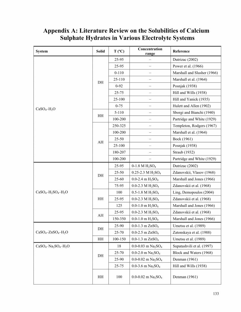
133

Appendix A: Literature Review on the Solubilities of Calcium Sulphate Hydrates in Various Electrolyte Systems

System Solid T (ºC) Concentration range Reference

25-95 – Dutrizac (2002)

25-95 – Power et al. (1966)

0-110 – Marshall and Slusher (1966)

25-110 – Marshall et al. (1964)

0-92 – Posnjak (1938)

25-75 – Hill and Wills (1938)

25-100 – Hill and Yanick (1935)

DH

0-75 – Hulett and Allen (1902)

5-110 – Sborgi and Bianchi (1940) HH

100-200 – Partridge and White (1929)

250-325 – Templeton, Rodgers (1967)

100-200 – Marshall et al. (1964)

25-50 – Bock (1961)

25-100 – Posnjak (1938)

180-207 – Straub (1932)

CaSO4–H2O

AH

100-200 – Partridge and White (1929)

25-95 0-1.8 M H2SO4 Dutrizac (2002)

25-50 0.25-2.3 M H2SO4 Zdanovskii, Vlasov (1968)

25-60 0.0-2.4 m H2SO4 Marshall and Jones (1966) DH

75-95 0.0-2.3 M H2SO4 Zdanovskii et al. (1968)

100 0.5-1.8 M H2SO4 Ling, Demopoulos (2004)

25-95 0.0-2.3 M H2SO4 Zdanovskii et al. (1968) HH

125 0.0-1.0 m H2SO4 Marshall and Jones (1966)

25-95 0.0-2.3 M H2SO4 Zdanovskii et al. (1968)

CaSO4–H2SO4–H2O

AH 150-350 0.0-1.0 m H2SO4 Marshall and Jones (1966)

25-90 0.0-1.3 m ZnSO4 Umetsu et al. (1989) DH

25-70 0.0-2.5 m ZnSO4 Zatonskaya et al. (1988) CaSO4–ZnSO4–H2O

HH 100-150 0.0-1.3 m ZnSO4 Umetsu et al. (1989)

18 0.0-0.03 m Na2SO4 Supatashvili et al. (1997)

25-70 0.0-2.0 m Na2SO4 Block and Waters (1968)

25-90 0.0-0.02 m Na2SO4 Denman (1961) DH

25-75 0.0-3.6 m Na2SO4 Hill and Wills (1938)

CaSO4–Na2SO4–H2O

HH 100 0.0-0.02 m Na2SO4 Denman (1961)

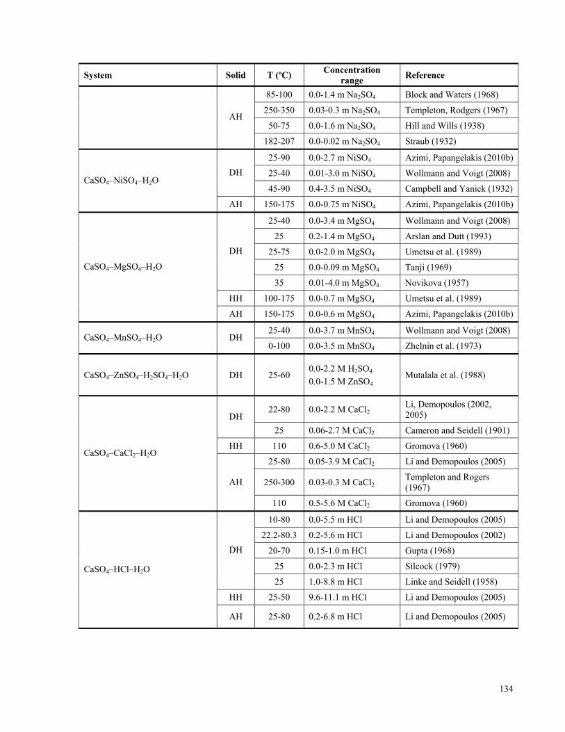
134

System Solid T (ºC) Concentration range Reference

85-100 0.0-1.4 m Na2SO4 Block and Waters (1968)

250-350 0.03-0.3 m Na2SO4 Templeton, Rodgers (1967)

50-75 0.0-1.6 m Na2SO4 Hill and Wills (1938) AH

182-207 0.0-0.02 m Na2SO4 Straub (1932)

25-90 0.0-2.7 m NiSO4 Azimi, Papangelakis (2010b)

25-40 0.01-3.0 m NiSO4 Wollmann and Voigt (2008) DH

45-90 0.4-3.5 m NiSO4 Campbell and Yanick (1932) CaSO4–NiSO4–H2O

AH 150-175 0.0-0.75 m NiSO4 Azimi, Papangelakis (2010b)

25-40 0.0-3.4 m MgSO4 Wollmann and Voigt (2008)

25 0.2-1.4 m MgSO4 Arslan and Dutt (1993)

25-75 0.0-2.0 m MgSO4 Umetsu et al. (1989)

25 0.0-0.09 m MgSO4 Tanji (1969)

DH

35 0.01-4.0 m MgSO4 Novikova (1957)

HH 100-175 0.0-0.7 m MgSO4 Umetsu et al. (1989)

CaSO4–MgSO4–H2O

AH 150-175 0.0-0.6 m MgSO4 Azimi, Papangelakis (2010b)

25-40 0.0-3.7 m MnSO4 Wollmann and Voigt (2008) CaSO4–MnSO4–H2O DH

0-100 0.0-3.5 m MnSO4 Zhelnin et al. (1973)

CaSO4–ZnSO4–H2SO4–H2O DH 25-60 0.0-2.2 M H2SO4

0.0-1.5 M ZnSO4 Mutalala et al. (1988)

22-80 0.0-2.2 M CaCl2 Li, Demopoulos (2002, 2005) DH

25 0.06-2.7 M CaCl2 Cameron and Seidell (1901)

HH 110 0.6-5.0 M CaCl2 Gromova (1960)

25-80 0.05-3.9 M CaCl2 Li and Demopoulos (2005)

250-300 0.03-0.3 M CaCl2 Templeton and Rogers (1967)

CaSO4–CaCl2–H2O

AH

110 0.5-5.6 M CaCl2 Gromova (1960)

10-80 0.0-5.5 m HCl Li and Demopoulos (2005)

22.2-80.3 0.2-5.6 m HCl Li and Demopoulos (2002)

20-70 0.15-1.0 m HCl Gupta (1968)

25 0.0-2.3 m HCl Silcock (1979)

DH

25 1.0-8.8 m HCl Linke and Seidell (1958)

HH 25-50 9.6-11.1 m HCl Li and Demopoulos (2005)

CaSO4–HCl–H2O

AH 25-80 0.2-6.8 m HCl Li and Demopoulos (2005)

135

System Solid T (ºC) Concentration range Reference

10-110 0.0-4.7 m NaCl Marshall and Slusher (1966)

28-90 0.0-5.5 m NaCl Ostroff and Metler (1966)

25-100 0.0-4.0 m NaCl Marshall et al. (1964) DH

15-50 0.0-4.4 m NaCl Silcock (1979)

HH 125 0.0-4.0 m NaCl Marshall et al. (1964)

100-300 0.0-6.0 m NaCl Blount and Dickson (1969)

250-325 0.0-5.7 m NaCl Templeton and Rogers (1967)

125-200 0.0-4.0 m NaCl Marshall et al. (1964)

25-50 0.0-5.0 m NaCl Bock (1961)

CaSO4–NaCl–H2O

AH

125-200 0.9-5.5 m NaCl Silcock (1979)

25 0.0-5.3 m MgCl2 Zdanovskii, Chernova (1976)

38-70 0.0-0.35 m MgCl2 Ostroff and Metler (1966)

25 0.0-5.0 m MgCl2 Linke and Seidell (1958) DH

25 0.0-5.3 m MgCl2 Cameron and Seidell (1901)

CaSO4–MgCl2–H2O

AH 250-300 0.03-0.3 m MgCl2 Templeton, Rogers (1967)

CaSO4–AlCl3–H2O DH 25-80 0.0-1.5 m AlCl3 Li and Demopoulos (2006a)

CaSO4–FeCl3–HCl–H2O DH 25-80 0.0-2.2 m FeCl3

0.5, 3.0 m HCl Li and Demopoulos (2006a)

22-80 0.0-2.2 m CaCl2

1.0, 3.0, 5.0 m HCl Li and Demopoulos (2005)

22.2-80.3 0.01-2.1 m CaCl2

1.0 m HCl Li and Demopoulos (2002) DH

20 0.0-3.0 m CaCl2

0.0-6.0 m HCl Silcock (1979)

HH 60-80 0.05-4.7 m CaCl2

3.0, 6.0 m HCl Li and Demopoulos (2005)

CaSO4–CaCl2–HCl–H2O

AH 25-80 0.05-4.3 m CaCl2

3.0, 6.0 m HCl Li and Demopoulos (2005)

136

System Solid T (ºC) Concentration range Reference

25-80 0.7-3.3 m MgCl2

0.5 m HCl Li and Demopoulos (2006a)

50-80 0.0-2.2 m MgCl2

0.5 m HCl Li and Demopoulos (2002) DH

25-50 0.3-3.5 m MgCl2

3.0 m HCl Li and Demopoulos (2006a)

CaSO4–MgCl2–HCl–H2O

AH 80 0.3-3.5 m MgCl2

3.0 m HCl Li and Demopoulos (2006a)

CaSO4–NaCl–HCl–H2O DH 50-80 0.5-3.0 m NaCl

0.5 m HCl Li and Demopoulos (2006a)

DH 50 0.2-1.5 m CaCl2

1.0 m MgCl2

0.5 m HCl Li and Demopoulos (2006a)

CaSO4–CaCl2–MgCl2–HCl–H2O

HH 60 0.3-1.9 m CaCl2

1.0 m MgCl2

6.0 m HCl Li and Demopoulos (2006a)

25 0.0-5.9 m Na2SO4

0.0-1.9 m NaCl Yeatts and Marshall (1972)

25-70 0.0-2.0 m Na2SO4

0.0-4.0 m NaCl Block and Waters (1968) DH

25 0.4-1.8 m Na2SO4

0.5-5.6 m NaCl Cameron et al. (1907)

85-100 0.0-1.1 m Na2SO4

0.5-2.0 m NaCl Block and Waters (1968)

100 0.01-0.03 m Na2SO4

2.0 m NaCl Furby et al. (1968)

CaSO4–Na2SO4–NaCl–H2O

AH

250-300 0.0-0.3 m Na2SO4

0.0-0.9 m NaCl Templeton, Rodgers (1967)

CaSO4–Na2SO4–MgCl2–H2O DH 40 0.0-2.0 m Na2SO4

0.0-0.6 m MgCl2 Barba et al. (1984)

DH 28-250 0.0-5.5 m NaCl

0.0-4.4 m MgCl2 Ostroff and Metler (1966)

CaSO4–NaCl–MgCl2–H2O AH 250-300

0.0-0.5 m NaCl

0.0-0.16 m MgCl2 Templeton, Rodgers (1967)

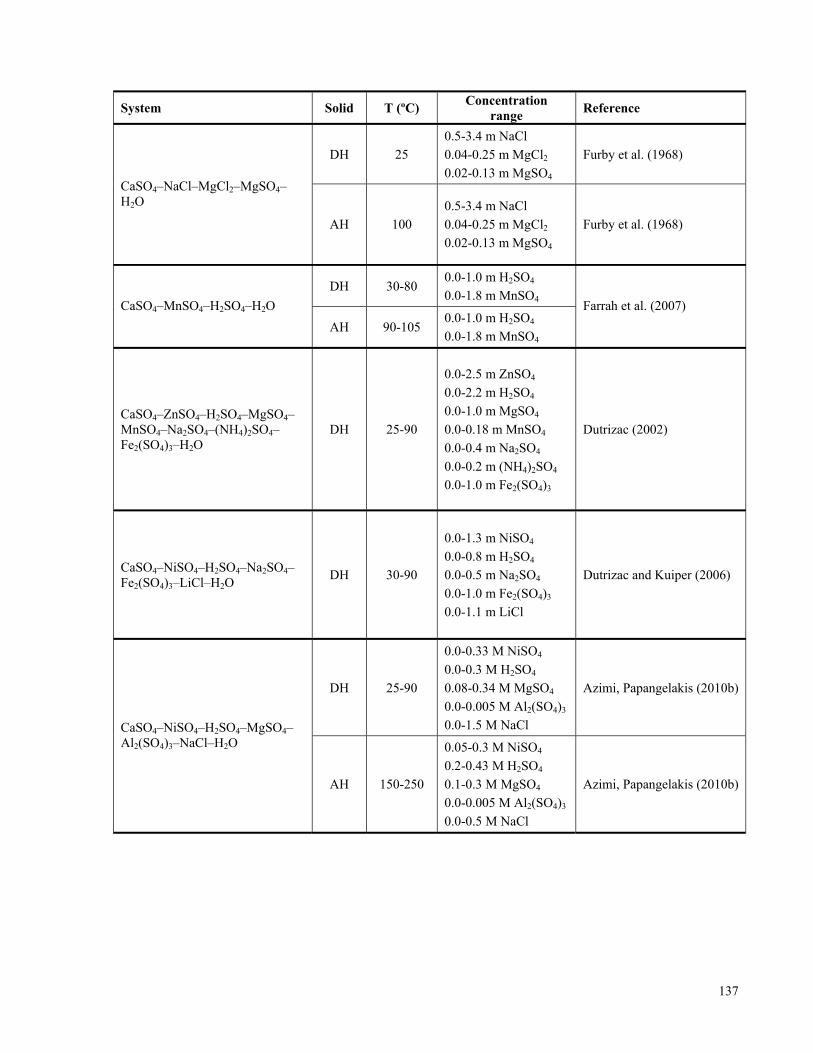
137

System Solid T (ºC) Concentration range Reference

DH 25 0.5-3.4 m NaCl

0.04-0.25 m MgCl2

0.02-0.13 m MgSO4

Furby et al. (1968)

CaSO4–NaCl–MgCl2–MgSO4–H2O

AH 100 0.5-3.4 m NaCl

0.04-0.25 m MgCl2

0.02-0.13 m MgSO4 Furby et al. (1968)

DH 30-80 0.0-1.0 m H2SO4

0.0-1.8 m MnSO4 CaSO4–MnSO4–H2SO4–H2O AH 90-105

0.0-1.0 m H2SO4

0.0-1.8 m MnSO4

Farrah et al. (2007)

CaSO4–ZnSO4–H2SO4–MgSO4–MnSO4–Na2SO4–(NH4)2SO4–Fe2(SO4)3–H2O

DH 25-90

0.0-2.5 m ZnSO4

0.0-2.2 m H2SO4

0.0-1.0 m MgSO4

0.0-0.18 m MnSO4

0.0-0.4 m Na2SO4

0.0-0.2 m (NH4)2SO4

0.0-1.0 m Fe2(SO4)3

Dutrizac (2002)

CaSO4–NiSO4–H2SO4–Na2SO4–Fe2(SO4)3–LiCl–H2O DH 30-90

0.0-1.3 m NiSO4

0.0-0.8 m H2SO4

0.0-0.5 m Na2SO4

0.0-1.0 m Fe2(SO4)3

0.0-1.1 m LiCl

Dutrizac and Kuiper (2006)

DH 25-90

0.0-0.33 M NiSO4

0.0-0.3 M H2SO4

0.08-0.34 M MgSO4

0.0-0.005 M Al2(SO4)3

0.0-1.5 M NaCl

Azimi, Papangelakis (2010b)

CaSO4–NiSO4–H2SO4–MgSO4–Al2(SO4)3–NaCl–H2O

AH 150-250

0.05-0.3 M NiSO4

0.2-0.43 M H2SO4

0.1-0.3 M MgSO4

0.0-0.005 M Al2(SO4)3

0.0-0.5 M NaCl

Azimi, Papangelakis (2010b)

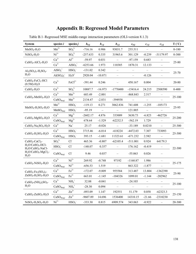
138

Appendix B: Regressed Model Parameters Table B.1–Regressed MSE middle-range interaction parameters (OLI-version 8.1.3)

System species i species j b0,ij b1,ij b2,ij c0,ij c1,ij c2,ij T (˚C)

MnSO4-H2O Mn2+ SO42- -716.16 0.906 93031.7 255.511 – – 0-180

NiSO4-H2O Ni2+ SO42- -257.633 0.335 31965.6 301.129 -0.239 -31179.97 0-300

Ca2+ Al3+ -59.97 0.031 – -97.159 0.683 – CaSO4-AlCl3-H2O

Ca2+ AlSO4+ -6253.66 1.973 110385 1870.31 12.133 –

25-80

AlSO4+ HSO4

- -131.02 0.342 – – – – Al2(SO4)3-H2SO4-H2O Al(SO4)2

- H3O+ 2920.04 -10.871 – – -0.126 – 25-70

CaSO4-FeCl3-HCl (0.5M)-H2O Ca2+ FeCl2+ -391.44 0.246 – 450.167 0.004 – 20-80

CaSO4-H2O Ca2+ SO42- 10887.7 -16.973 -1770400 -15416.4 24.215 2508590 0-400

Ca2+ Mn2+ 683.49 -2.001 – -868.843 2.517 – CaSO4-MnSO4-H2O

CaSO4(aq) Mn2+ 2134.47 -2.831 -394938 – – – 25-100

Mn2+ HSO4- -119.13 0.271 3062.836 741.608 -1.255 -105173

MnSO4-H2SO4-H2O MnSO4(aq) HSO4

- -95.19 – – 121.885 – – 25-95

Ca2+ Mg2+ -2602.17 4.876 333009 3630.73 -6.823 -462726 CaSO4-MgSO4-H2O

CaSO4(aq) Mg2+ 678.64 -1.529 -62232.5 -562.19 1.729 – 25-200

CaSO4-Na2SO4-H2O Ca2+ Na+ 25.17 -0.026 – -33.189 0.0210 – 25-300

Ca2+ HSO4- 3715.46 -6.014 -618224 -4472.03 7.307 733093

CaSO4-H2SO4-H2O CaSO4(aq) HSO4

- 393.15 -1.681 11323.61 -671.232 2.582 – 25-300

SO42- Cl- 465.36 -0.807 -62105.4 -511.001 0.924 64179.3

HSO4- Cl- -148.07 0.357 – 176.162 -0.419 –

CaSO4-CaCl2-H2O/CaSO4-HCl-H2O/CaSO4-NaCl-H2O/CaSO4-MgCl2-H2O CaSO4(aq) Cl- 9.46 0.037 – -55.063 0.026 –

22-300

Ca2+ Ni2+ 269.92 -0.748 97192 -1160.87 1.986 – CaSO4-NiSO4-H2O

CaSO4(aq) Ni2+ -656.53 1.519 – 863.322 -1.877 – 25-175

Ca2+ Fe3+ -172.07 -9.809 955584 313.487 13.804 -1362390 CaSO4-Fe2(SO4)3-ZnSO4-H2SO4-H2O CaSO4(aq) Fe3+ 663.01 -1.145 -104326 1099.01 -1.144 -202962

25-90

Ca2+ NH4+ 32.88 -0.041 – -24.103 – – CaSO4-(NH4)2SO4-

H2O CaSO4(aq) NH4+ -28.30 0.094 – – – –

25-100

Ca2+ Zn2+ -893.09 1.147 192551 51.179 0.058 -62323.3 CaSO4-ZnSO4-H2O

CaSO4(aq) Zn2+ -9607.89 14.696 1536400 14310.15 -21.66 -2310230 25-150

NiSO4-H2SO4-H2O Ni2+ HSO4- -333.30 0.815 6909.574 343.063 -0.922 – 20-300

139

Table B.2–Regressed standard state Gibbs free energy and entropy of formation of various solids in comparison with the literature data

From literature Regressed values

Lange's Handbook / Golam Mostafa (1995) error%*

Solids ΔGf

º Sfº ΔGf

º Sfº ΔGf

º Sfº

T (°C)

CaSO4•0.5H2O -343903 31.479 -343732 / -322875 31.22 / 31.34 0.05/6.5 0.83/0.43 0–200 NiSO4•7H2O -588592 95.807 -589043 / -599260 90.66 / 94.18 0.08/1.78 5.68/1.72 0–32 NiSO4•6H2O -531852 80.678 -531000 / -540811 75.10 / 83.67 0.16/1.65 7.43/3.57 32–100 NiSO4•1H2O -244864 30.956 – / -248566 – / 31.11 – /1.49 – /0.49 100–220 MnSO4•7H2O -632452 114.66 – / -639346 – / 111.8 – /1.08 – /2.52 0–10 MnSO4•5H2O -518996 81.760 – / -522448 – / 81.02 – /0.66 – /0.91 10–25 MnSO4•1H2O -291986 22.136 – / -288652 – / 26.72 – /1.15 – /17.0 25–180

*100% ×

−=

valueliterature

valueliteraturevalueregressederror

140

Appendix C: Experimental Measurements in Laterite PAL Solutions

Table C.1 – Solubility of CaSO4 dihydrate (gypsum) in water at various NiSO4 concentrations

25°C 45°C 70°C 90°C NiSO4 CaSO4 density* CaSO4 density* CaSO4 density* CaSO4 density* mol/L mol/L g/mL mol/L g/mL mol/L g/mL mol/L g/mL

0.0 0.0154 0.998 0.0153 0.990 0.0146 0.974 0.0136 0.970 0.1 0.0110 1.014 0.0117 1.009 0.0117 1.001 0.0117 0.983 0.5 0.0128 1.075 0.0140 1.070 0.0160 1.060 0.0163 1.045 1.1 0.0145 1.148 0.0166 1.138 0.0183 1.130 0.0202 1.115 1.6 0.0143 1.216 0.0161 1.203 0.0188 1.192 0.0214 1.177 2.1 - - 0.0147 1.270 0.0184 1.253 0.0218 1.236 2.7 - - 0.0121 1.354 0.0154 1.321 0.0182 1.300

*density at temperature

Table C.2 – Solubility of CaSO4 anhydrite in water at various NiSO4 concentrations

150°C 175°C NiSO4 CaSO4 density* CaSO4 density* mol/L mol/L g/ml mol/L g/ml

0.0 0.0017 0.997 0.0010 0.997 0.1 0.0014 1.013 0.0009 1.013 0.3 0.0021 1.041 0.0012 1.039 0.6 0.0029 1.085 0.0019 1.084 0.8 0.0036 1.130 0.0026 1.127

*density at 25°C

Table C.3 – Solubility of CaSO4 anhydrite in water at various MgSO4 concentrations

150°C 175°C MgSO4 CaSO4 density* CaSO4 density* mol/L mol/L g/mL mol/L g/mL

0.00 0.0017 0.997 0.0010 0.997 0.10 0.0014 1.010 0.0008 1.010 0.20 0.0018 1.022 0.0010 1.022 0.40 0.0023 1.045 0.0014 1.045 0.60 0.0029 1.065 0.0020 1.065

*density at 25°C

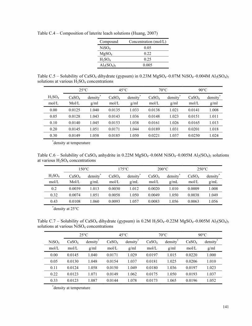
141

Table C.4 – Composition of laterite leach solutions (Huang, 2007)

Compound Concentration (mol/L) NiSO4 0.05 MgSO4 0.22 H2SO4 0.25 Al2(SO4)3 0.005

Table C.5 – Solubility of CaSO4 dihydrate (gypsum) in 0.23M MgSO4–0.07M NiSO4–0.004M Al2(SO4)3 solutions at various H2SO4 concentrations

25°C 45°C 70°C 90°C

H2SO4 CaSO4 density* CaSO4 density* CaSO4 density* CaSO4 density*

mol/L Mol/L g/ml mol/L g/ml mol/L g/ml mol/L g/ml

0.00 0.0125 1.040 0.0135 1.033 0.0138 1.021 0.0141 1.008 0.05 0.0128 1.043 0.0143 1.036 0.0148 1.023 0.0151 1.011 0.10 0.0140 1.045 0.0153 1.038 0.0161 1.026 0.0165 1.013 0.20 0.0145 1.051 0.0171 1.044 0.0189 1.031 0.0201 1.018 0.30 0.0149 1.058 0.0185 1.050 0.0221 1.037 0.0250 1.024

*density at temperature

Table C.6 – Solubility of CaSO4 anhydrite in 0.22M MgSO4–0.06M NiSO4–0.005M Al2(SO4)3 solutions at various H2SO4 concentrations

150°C 175°C 200°C 250°C H2SO4 CaSO4 density* CaSO4 density* CaSO4 density* CaSO4 density* mol/L Mol/L g/mL mol/L g/mL mol/L g/mL mol/L g/mL

0.2 0.0039 1.013 0.0030 1.012 0.0020 1.010 0.0009 1.008 0.32 0.0074 1.051 0.0058 1.050 0.0049 1.050 0.0038 1.049 0.43 0.0108 1.060 0.0093 1.057 0.0083 1.056 0.0063 1.056

*density at 25°C

Table C.7 – Solubility of CaSO4 dihydrate (gypsum) in 0.2M H2SO4–0.22M MgSO4–0.005M Al2(SO4)3 solutions at various NiSO4 concentrations

25°C 45°C 70°C 90°C

NiSO4 CaSO4 density* CaSO4 density* CaSO4 density* CaSO4 density* mol/L mol/L g/ml mol/L g/ml mol/L g/ml mol/L g/ml

0.00 0.0145 1.040 0.0171 1.029 0.0197 1.015 0.0220 1.000 0.05 0.0130 1.048 0.0154 1.037 0.0181 1.025 0.0206 1.010 0.11 0.0124 1.058 0.0150 1.049 0.0180 1.036 0.0197 1.023 0.22 0.0123 1.071 0.0149 1.062 0.0175 1.050 0.0193 1.037 0.33 0.0123 1.087 0.0144 1.078 0.0173 1.065 0.0196 1.052

*density at temperature

142

Table C.8 – Solubility of CaSO4 anhydrite in 0.3M H2SO4–0.22M MgSO4–0.005M Al2(SO4)3 solutions at various NiSO4 concentrations

150°C 175°C 200°C

NiSO4 CaSO4 density* CaSO4 density* CaSO4 density* mol/L mol/L g/ml mol/L g/ml mol/L g/ml

0.05 0.0072 1.049 0.0058 1.048 0.0048 1.048 0.10 0.0065 1.055 0.0052 1.055 0.0043 1.054 0.20 0.0056 1.075 0.0042 1.071 0.0032 1.071 0.30 0.0057 1.087 0.0041 1.086 0.0030 1.084 *density at 25°C

Table C.9 – Solubility of CaSO4 dihydrate (gypsum) in 0.2M H2SO4–0.05M NiSO4–0.005M Al2(SO4)3 solutions at various MgSO4 concentrations

25°C 45°C 70°C 90°C

MgSO4 CaSO4 density* CaSO4 density* CaSO4 density* CaSO4 density* mol/L Mol/L g/mL mol/L g/mL mol/L g/mL mol/L g/mL

0.08 0.0125 1.033 0.0149 1.022 0.0187 1.010 0.0226 1.000 0.16 0.0120 1.043 0.0144 1.033 0.0171 1.020 0.0190 1.006 0.25 0.0121 1.055 0.0140 1.043 0.0157 1.028 0.0175 1.015 0.34 0.0121 1.065 0.0136 1.054 0.0154 1.040 0.0169 1.025

*density at temperature

Table C.10 – Solubility of CaSO4 anhydrite in 0.3M H2SO4–0.06M NiSO4–0.005M Al2(SO4)3 solutions at various MgSO4 concentrations

150°C 175°C 200°C 250°C

MgSO4 CaSO4 density* CaSO4 density* CaSO4 density* CaSO4 density* mol/L Mol/L mg/L mol/L mg/L mol/L mg/L mol/L mg/L

0.1 0.0106 1.038 0.0093 1.038 0.0079 1.038 0.0059 1.039 0.2 0.0075 1.048 0.0059 1.048 0.0047 1.047 0.0030 1.050 0.3 0.0053 1.054 0.0042 1.055 0.0030 1.056 0.0020 1.058 *density at 25°C

143

Table C.11 – Solubility of CaSO4 anhydrite in 0.25M H2SO4–0.2M MgSO4–0.005M Al2(SO4)3–0.05M NiSO4 solutions at 0.0 and 0.5M NaCl concentrations

T H2SO4 MgSO4 Al2(SO4)3 NiSO4 NaCl CaSO4 density* °C mol/L mol/L mol/L mol/L mol/L mol/L g/mL

150 0.22 0.2 0.005 0.06 0 0.0039 1.013 175 0.22 0.2 0.005 0.06 0 0.0030 1.012 200 0.22 0.2 0.005 0.06 0 0.0020 1.010 250 0.22 0.2 0.005 0.06 0 0.0009 1.008 150 0.25 0.2 0.004 0.05 0.5 0.0066 1.065 175 0.25 0.2 0.004 0.05 0.5 0.0055 1.064 200 0.25 0.2 0.004 0.05 0.5 0.0042 1.063 250 0.25 0.2 0.004 0.05 0.5 0.0028 1.063 *density at 25°C

Table C.12 – Solubility of CaSO4 dihydrate (gypsum) in 0.5M H2SO4 solutions at various NaCl concentrations

25°C 45°C 70°C 90°C NaCl CaSO4 density* CaSO4 density* CaSO4 density* CaSO4 density* mol/L mol/L g/mL mol/L g/mL mol/L g/mL mol/L g/mL

0.0 0.0193 1.030 0.0260 1.023 0.0403 1.015 0.0545 1.000 0.1 0.0200 1.034 0.0281 1.027 0.0409 1.016 0.0541 1.007 0.5 0.0235 1.050 0.0321 1.042 0.0444 1.033 0.0620 1.024 1.0 0.0248 1.068 0.0338 1.062 0.0506 1.056 0.0667 1.043 1.5 0.0263 1.090 0.0359 1.078 0.0537 1.071 0.0719 1.060

*density at temperature

144

Table C.13 – Solubility of CaSO4 dihydrate in 0.5M HCl solutions at various MgSO4 concentrations

25°C 45°C 70°C 90°C MgSO4 CaSO4 density* CaSO4 density* CaSO4 Density CaSO4 density* mol/L mol/L g/mL mol/L g/mL mol/L g/mL mol/L g/mL

0.0 0.0810 1.007 0.0940 1.005 0.1300 1.004 0.1560 0.997 0.1 0.0456 1.021 0.0594 1.013 0.0785 1.008 0.0987 0.999 0.5 0.0168 1.057 0.0205 1.047 0.0231 1.038 0.0292 1.030 1.0 0.0110 1.112 0.0139 1.100 0.0153 1.105 0.0188 1.080 1.5 0.0087 1.162 0.0105 1.158 0.0113 1.102 0.0135 1.128

*density at temperature

Table C.14 – Solubility of CaSO4 dihydrate in 0.5M H2SO4 solutions at various NiSO4 concentrations

25°C 45°C 70°C 90°C NiSO4 CaSO4 density* CaSO4 density* CaSO4 density* CaSO4 density* mol/L mol/L g/mL mol/L g/mL mol/L g/mL mol/L g/mL

0.00 0.0190 1.030 0.0258 1.022 0.0403 1.010 0.0545 1.002 0.10 0.0180 1.044 0.0234 1.037 0.0351 1.026 0.0454 1.015 0.25 0.0166 1.060 0.0210 1.056 0.0298 1.044 0.0383 1.029 0.50 0.0166 1.106 0.0196 1.095 0.0266 1.085 0.0329 1.071 1.00 0.0148 1.180 0.0172 1.170 0.0234 1.157 0.0314 1.141 1.50 0.0131 1.238 0.0158 1.230 0.0194 1.218 0.0245 1.202

*density at temperature

145

Appendix D: X-ray Diffraction Patterns

Figure D.1 X-ray diffraction pattern of the gypsum feed.

Figure D.2 X-ray diffraction pattern of the anhydrite feed (AII).

146

Figure D.3 X-ray diffraction pattern of hemihydrate*.

Figure D.4 X-ray diffraction pattern of soluble (AIII or γ) anhydrite (obtained from the ICDD, Bushuev et al., 1983). * Note: this XRD pattern is collected from a solid sample obtained in this work from gypsum dehydration

in pure water at 150°C inside an autoclave after 3 h. No hemihydrate was detected in the experiments carried out below 100°C.

147

XRD Patterns of the Solids in H2SO4 media at 70°C after 3 h

Figure D.5 X-ray diffraction pattern of the equilibrating solid phase in H2SO4 media at 70°C (retention time=3 h): (a) 2θ = 10–55° (b) 2θ = 37–44°. SEM image of this solid is presented in Fig. 5.14 (b).

no AII-AH characteristic peak

b

a

148

XRD Patterns of the Solids in H2SO4 media at 70°C after 12 days

Figure D.6 X-ray diffraction pattern of the equilibrating solid phase in H2SO4 media at 70°C (retention time=12 days): (a) 2θ = 10–60° (b) 2θ = 31–45°. SEM image of this solid is presented in Fig. 5.14 (c).

Characteristic Peak of AII-AH

a

b

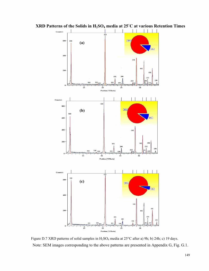
149

XRD Patterns of the Solids in H2SO4 media at 25˚C at various Retention Times

Figure D.7 XRD patterns of solid samples in H2SO4 media at 25°C after a) 9h; b) 24h; c) 19 days.

Note: SEM images corresponding to the above patterns are presented in Appendix G, Fig. G.1.

(a)

(b)

(c)

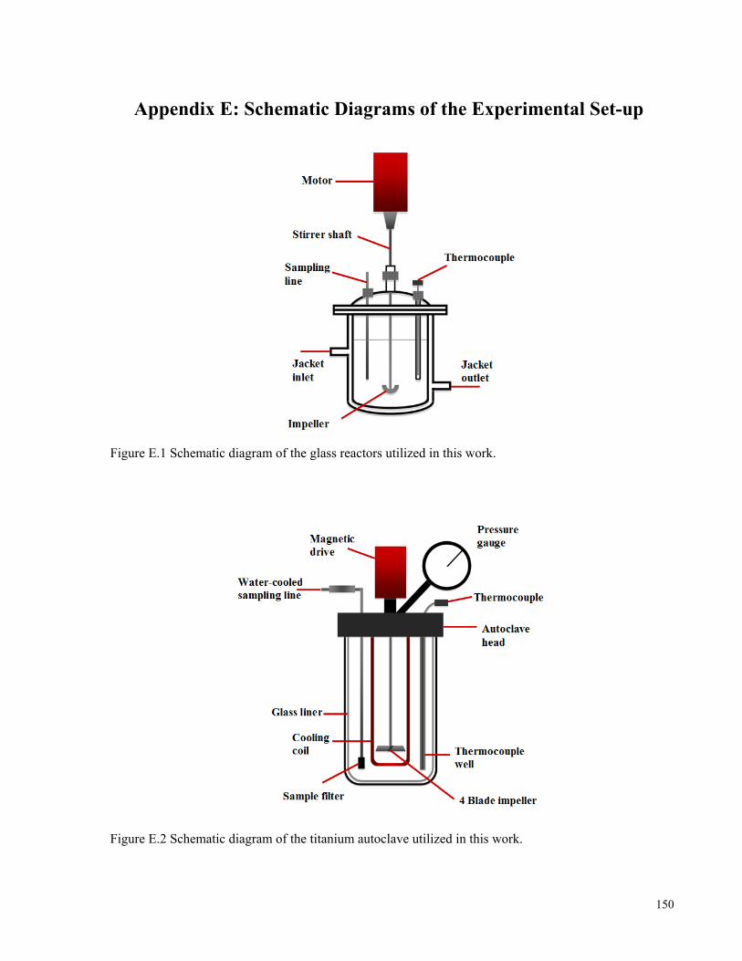
150

Appendix E: Schematic Diagrams of the Experimental Set-up

Figure E.1 Schematic diagram of the glass reactors utilized in this work.

Figure E.2 Schematic diagram of the titanium autoclave utilized in this work.

151

Appendix F: Experimental Measurements for DH-AH transformation

Table F.1– Gypsum–anhydrite transformation at 90°C in water (starting with 50 g/L gypsum+5 g/L anhydrite seeds as the saturating solid phase)

Solid% Sample ID Time (days) Gypsum Anhydrite #1 0.4 88 12 #2 1.0 90 10 #3 1.3 89 11 #4 1.9 90 10 #5 2.9 89 11 #6 5.0 60 40 #7 5.3 55 45 #8 7.3 27 73 #9 8.3 7 93 #10 9.8 0 100 #11 12.1 0 100 #12 13.1 0 100 #13 14.2 0 100

Table F.2– Concentration of CaSO4 and composition of saturating solid phases at various temperatures and residence times in 0.5 and 1.0 M H2SO4 solutions

[H2SO4]=0.5 M [H2SO4]=1.0 M Time

CaSO4 Solid (%) CaSO4 Solid (%) Sample ID

h Day T/°C Method

mol/L DH AH mol/L DH AH

#1 0 0 25 Heating – 100 0 – 100 0 #2 26 1 25 Heating 0.0187 95 5 0.0189 90 10 #3 50 2 45 Heating 0.0273 95 5 0.0288 90 10 #4 98 4 45 Heating 0.0271 95 5 0.0286 90 10 #5 122 5 60 Heating 0.0360 95 5 0.0391 90 10 #6 145 6 70 Heating 0.0417 95 5 0.0464 90 10 #7 169 7 70 Heating 0.0423 95 5 0.0471 90 10 #8 192 8 80 Heating 0.0506 95 5 0.0559 80 20 #9 264 11 90 Heating 0.0623 25 75 0.0581 0 100

#10 288 12 90 Heating 0.0455 0 100 0.0379 0 100 #11 315 13 70 Cooling 0.0422 0 100 0.0357 0 100 #12 344 14 45 Cooling 0.0295 15 85 0.0315 0 100 #13 390 16 25 Cooling 0.0193 100 0 0.0177 30 70

152

Table F.3– Concentration of CaSO4 and composition of saturating solid phases at various temperatures and residence times in 1.5 and 2.0 M H2SO4 solutions

[H2SO4]=1.5 M [H2SO4]=2.0 M Time

CaSO4 Solid (%) CaSO4 Solid (%) Sample ID

h day T/°C Method

mol/L DH AH mol/L DH AH

#1 0 0 25 – – 100 0 – 100 0 #2 24 1 25 Heating 0.0179 85 15 0.0154 85 15 #3 50 2 45 Heating 0.0284 85 15 0.0246 82 18 #4 70 3 45 Heating 0.0285 85 15 0.0251 85 15 #5 94 4 60 Heating 0.0392 85 15 0.0357 85 15 #6 151 6 60 Heating 0.0391 85 15 0.0347 82 18 #7 171 7 70 Heating 0.0495 85 15 0.0466 82 18 #8 192 8 70 Heating 0.0502 85 15 0.0449 82 18 #9 216 9 70 Heating 0.0476 80 20 0.0456 70 30

#10 245 10 80 Heating 0.0600 80 20 0.0451 0 100 #11 266 11 80 Heating 0.0617 60 40 0.0321 0 100 #12 293 12 80 Heating 0.0461 0 100 0.0317 0 100 #13 359 15 90 Heating 0.0353 0 100 0.0274 0 100 #14 383 16 70 Cooling 0.0338 0 100 0.0245 0 100 #15 407 17 45 Cooling 0.0319 0 100 0.0232 0 100 #16 435 18 25 Cooling 0.0173 15 85 0.0131 5 95

* DH: gypsum, AH: anhydrite

153

Appendix G: Additional SEM Images

Solid samples in H2SO4 media at 25˚C at various retention times

Figure G.1 SEM images of solid samples in 1.5 M H2SO4 media at 25°C after a) 9h; b) 24h; c) and d) 19 days.

Note: XRD patterns corresponding to the above SEM images are presented in Appendix D, Fig. D.7.

a

b

c d

154

SEM images of solid samples in pure water at 90˚C at various retention times

Following SEM images present solid samples in pure water at 90°C, in the absence of anhydrite

seeds, at various retention times. X-ray diffraction analysis showed 100% gypsum for all the

solids.

t=6 h t=46 h

t=121 h t=175 h Figure G.2 SEM images of saturating solid samples in pure water at 90°C after various retention times (in the absence of anhydrite seeds).

(a) (b)

(c) (d)

155

Appendix H: The Rietveld Method (Full-Pattern Analysis)

In the present work, the quantification of XRD patterns were performed utilizing the Rietveld

refinement (or Rietveld method), which is embedded in the XRD HighScore Software used to

analyze the diffractograms. Rietveld refinement is a computer-based analytical procedure,

pioneered by Hugo Rietveld (1969), for the characterization and quantification of crystalline

materials, utilizing the full information (such as intensities height and width as well as the

position of the reflections) over the powder pattern.

The Rietveld method was originally developed as a method of refining crystal structures using

neutron powder diffraction data. The method requires knowledge of the approximate crystal

structure of all phases of interest in the pattern. In this method, a full-pattern fit is done until a

theoretical profile matches the measured profile. In the Rietveld method, the basic approach is

to, first, obtain the X-ray pattern of the sample, and then to identify all phases present (using

available databases such as ICDD) and to input basic structural data for all the phases. After

that, the data are processed until the best fit to the experimental pattern is obtained. The quantity

minimized in Rietveld refinement is the conventional least squares residual:

2

)()(∑ −=j

cjojj IIwR

where Ij(o) and Ij(c) are the intensities observed and calculated, respectively, at the jth step in the

data, and wj is the weight at the jth step. Detailed discussion of the Rietveld method is beyond

the scope of this work, however, it is important to mention that this method is more accurate

compared to other available quantification methods such as peak intensity-based methods,

because of the whole-pattern fitting approach.

The Variables of a Rietveld Refinement:

The following variables are refined in the Rietveld method for the characterization of the

measured profiles:

• Peak shape function (which describes the shape of the diffraction peaks, e.g., Gaussian

shape);

156

• Peak width function (starts with optimal full width at half maximum (FWHM) values);

• Preferred orientation function (introduces a factor based on deviation from randomness);

• The structure factor (calculated from the crystal structure data and includes site

occupancy information, cell dimensions, inter-atomic distances, temperature and

magnetic factors. Crystal structure data is usually obtained from the ICDD database);

• The scale factor (relating the intensity of the experimental data with that of the model

data).

The least-squares parameters are those varied in the model to achieve the best fit to the

experimental data. In the Rietveld method, these parameters are divided into two groups. The

first group includes the profile parameters, defining the positions, half-widths, possible

asymmetry of the diffraction peaks, and preferred orientation. The second group contains the

structure parameters, defining the contents of the asymmetric unit cell, such as overall scale

factor, overall isotropic temperature parameter, and coordinates of all atomic units. More details

regarding the Rietveld refinements are available in the literature (Rietveld, 1969).

In the present work, the accuracy of the Rietveld method was validated against mixtures of

gypsum and anhydrite feed with known composition. The estimated compositions, from the

Rietveld refinement, and the measured compositions were in good agreement (AARD%= 7.3 for

gypsum and 10.4 for anhydrite), as shown in the following table:

Table H.1– Estimated vs. measured composition of the mixtures of gypsum/anhydrite solid samples

Measured composition, wt%

Rietveld estimated composition, wt% Relative Error, % Sample

ID gypsum anhydrite gypsum anhydrite gypsum anhydrite

#1 100 0 100 0 0.0 0.0 #2 90 10 85 15 5.6 50.0 #3 80 20 77 23 3.8 15.0 #4 70 30 69 31 1.4 3.3 #5 50 50 46 54 8.0 8.0 #6 35 65 35 65 0.0 0.0 #7 15 85 9 91 40.0 7.1 #8 0 100 0 100 0.0 0.0

AARD% – – – – 7.3 10.4

∑−

=NP

i valueExp

valueCalculatedvalueExp

NPAARD

.

.100(%)