Embed Size (px)
Citation preview
applied sciences
Article
Evaluating the Impact of Turbulence Closure Modelson Solute Transport Simulations in MeanderingOpen Channels
Jun Song Kim 1,2, Donghae Baek 3 and Inhwan Park 4,*1 Department of Earth and Environmental Sciences, University of Minnesota, Minneapolis, MN 55455, USA;
[email protected] Saint Anthony Falls Laboratory, University of Minnesota, Minneapolis, MN 55414, USA3 Department of Civil and Environmental Engineering, Seoul National University, Seoul 08826, Korea;
[email protected] Department of Civil Engineering, Seoul National University of Science and Technology, Seoul 01811, Korea* Correspondence: [email protected]; Tel.: +82-2-970-6507
Received: 24 March 2020; Accepted: 15 April 2020; Published: 16 April 2020�����������������
Abstract: River meanders form complex 3D flow patterns, including secondary flows and flowseparation. In particular, the flow separation traps solutes and delays their transport via storageeffects associated with recirculating flows. The simulation of the separated flows highly relies in theperformance of turbulence models. Thus, these closure schemes can control dispersion behaviorssimulated in rivers. This study performs 3D simulations to quantify the impact of the turbulencemodels on solute transport simulations in channels under different sinuosity conditions. The 3DReynolds-averaged Navier-Stokes equations coupled with the k− ε, k−ω and SST k−ω models areadopted for flow simulations. The 3D Lagrangian particle-tracking model simulates solute transport.An increase in sinuosity causes strong transverse gradients of mean velocity, thereby driving theonset of the separated flow recirculation along the outer bank. Here, the onset and extent of the flowseparation are strongly influenced by the turbulence models. The k− ε model fails to reproduce theflow separation or underestimates its size. As a result, the k− ε model yields residence times shorterthan those of other models. In contrast, the SST k−ω model exhibits a strong tailing of breakthroughcurves by generating more pronounced flow separation.
Keywords: meandering; flow separation; turbulence model; solute dispersion; storage zone
1. Introduction
River topography exerts a first-order control on flow and solute transport mechanisms. Especiallyin river bends, complex three-dimensional (3D) flow structures such as secondary flows and recirculatingflows develop due to the local imbalance between the centrifugal force and the pressure force [1,2].The velocity gradient driven by the secondary flow increases the longitudinal dispersion via shearflow effects [3]. The helical motion of the secondary flow not only impacts the primary flow but alsostimulates the transverse mixing [4,5]. Moreover, the dead zones with vigorous recirculating flows,developed by the channel irregularity, trap a solute cloud and induce the non-Fickian dispersioncharacterized as an elevated concentration of tracers downstream at late times [6,7]. Hence, theaforementioned flow features are required to be described adequately with numerical models foraccurate prediction of solute dispersion behaviors in surface water systems.
There have been numerous studies that use the 3D Reynolds-averaged Navier-Stokes (RANS)model for reproducing flow fields in large-scale meandering channels, honoring the reasonablecomputational cost compared to large eddy simulations (LES) and direct numerical simulations
Appl. Sci. 2020, 10, 2769; doi:10.3390/app10082769 www.mdpi.com/journal/applsci

Appl. Sci. 2020, 10, 2769 2 of 17
(DNS) [8–11]. The main advantage of the LES model is that the near-bank secondary flow within thechannel bend is superiorly reproduced compared to the RANS model [12,13]. The previous experimentalstudies; however, reported that the near-bank cell shrinks as the Froude number increases [14] andpossesses relatively weaker strength and smaller size than those of the main secondary flow cell at thecentral regions [15]. Therefore, in consideration of computational efficiency, the RANS model is anacceptable alternative for computing large-scale flow structures and shear flow dispersion accordinglyin meandering channels.
The flow structures simulated with the 3D RANS model substantially rely on turbulence models.Among several turbulence models, two-equation models are widely used for flow analysis. Since theresearch of Demuren and Rodi [16], the k − ε model has widely been employed for hydrodynamicsimulations in meander bends due to the computational stability with good convergence, adequatelycapturing entire flow patterns of the secondary circulations [17–20]. However, the k− ε model oftenfails to reproduce the adverse pressure gradient flows, thus causing inaccurate results in boundarylayer flows [21]. The k−ω model overcomes the disadvantages of the k− ε model by achieving moreprecise simulations in the wall boundary layers under the adverse pressure gradient conditions [22].Yet, both the k − ε and k −ω models lack the ability to reproduce massively separated flows undersevere adverse pressure gradients [23,24]. As an alternative to these turbulence models, Menter [25]proposed the shear stress transport (SST) k−ω model, which combines the robust formulations of thek −ω model for the near-wall regions and the k − ε model for the free-flow regions. The SST k −ωmodel has been shown to accurately predict the onset and extent of the flow separation in complexgeometric configurations [26–28].
In rivers and streams, the flow separation is frequently observed owing to the intricate flowpatterns associated with geomorphic features of rivers, such as confluence, pool-riffle sequence,bifurcation, and meander [29,30]. Notably, the experimental studies of Blanckaert [31–33] revealedthat sharp channel curvature forms a pronounced flow separation near the bend apex because ofsignificant adverse pressure gradients, and this curvature-induced flow separation manifests as arecirculation zone in the horizontal plane. The lateral recirculation zone (dead zone) acts as a surfacestorage zone, which induces anomalously long residence times of solutes via trapping effects, thendrive the non-Fickian tailing behaviors [34,35]. Thus, it is critical to accurately predict the onset andsize of the flow separation in meander bends for successfully capturing the non-Fickian transportsignatures in riverine environments. As aforementioned, the prediction of the flow separation is highlysensitive to turbulence models. The k− ε model has popularly been adopted for simulations of solutemixing in curved channels [16,36,37], whereas the impact of turbulence models on solute transport israrely assessed. Furthermore, the non-Fickian mixing properties associated with the horizontal flowrecirculation within the meander bend have not been deeply discussed with resepct to turbulencemodels and channel sinuosity.
The present work sheds light on the impact of turbulence closure models on solute transportand the non-Fickian mixing behaviors in meandering channels having different sinuosity levels. First,3D flow characteristics in meandering open channels are reproduced using the 3D RANS modelincorporated with a variety of turbulence closure schemes including the k − ε, k −ω and SST k −ωmodels. The flow simulation results are compared by changing meander geometry to scrutinize theinfluence of the turbulence models on the secondary flow and flow separation structures in channelsacross a diverse range of sinuosity. With the 3D flow fields obtained from the three different turbulencemodels, the solute transport is then simulated adopting the 3D Lagrangian particle-tracking (LPT)algorithm. This study eventually aims to unravel how the turbulence models influence the solutetransport simulations in meandering open-channel flows taking into account their performance inreproducing the meander-driven flow features, especially the separated flow recirculation.

Appl. Sci. 2020, 10, 2769 3 of 17
2. Methodology
2.1. Hydrodynamic Model
This study resolves 3D flow structures in meandering channels using the 3D RANS equations,which are solved with OpenFOAM, an open-source computational fluid dynamics library based on thefinite volume method. The OpenFOAM-based RANS models have been extensively used for analysisof open channel flows including bed erosion [28,38], hydraulic jump [39–41], spillway jet [41], flowsaround hydraulic structures [42–44], and coupled flows with porous media [45]. For incompressiblefluid flows, the 3D RANS model adopts the Reynold approximation of continuity and momentumequations as follows:
∂Ui∂xi
= 0 (1)
∂Ui∂t
+ U j∂Ui∂x j
= −1ρ∂P∂xi
+∂∂x j
[ν
(∂Ui∂x j
+∂U j
∂xi
)]−
∂∂x j
uiu j (2)
where Ui is the time-averaged velocity in the Cartesian coordinate; P is the pressure; ρ is the fluiddensity; ν is the kinematic viscosity; ui is the velocity fluctuation; and uiu j is the Reynolds stress. Underthe Boussinesq approximation, uiu j is defined as:
− uiu j = νt
(∂Ui∂x j
+∂U j
∂xi
)+
23
kδi j (3)
where νt is the turbulent eddy viscosity; k is the turbulent kinetic energy; δi j is the Kronecker delta.To close Equation (2) by resolving νt, this study employs two-equation turbulence closure models suchas k− ε, k−ω and SST k−ω models available with the Open FOAM library.
In the k − ε model, νt is modeled with the turbulent kinetic energy, k and the turbulent energydissipation, ε using the relation described as:
νt = ρCµk2
ε(4)
where Cµ is the empirical constant. The additional transport equations for simulating k and ε aregiven as:
∂k∂t
+∂(Uik)∂xi
=∂∂x j
[(νt
σk+ ν
)∂k∂x j
]− ε+ Gk (5)
∂ε∂t
+∂(Uiε)
∂xi=
∂∂x j
[(νt
σε+ ν
)∂ε∂x j
]+ Cε1Gk
εk−Cε2
ε2
k(6)
where σk, σε, Cε1, and Cε2 are the empirical constants; and Gk is the production of turbulent kineticenergy due to the mean velocity gradient. The empirical constants of the k− εmodel have been reportedas Cµ = 0.09, Cε1 = 1.44, Cε2 = 1.92, σk = 1.0, σε = 1.3 at high Reynolds number [46]. The k− ε modelis well known as the simplest turbulence model providing acceptable accuracy for diverse hydraulicproblems with good convergence. However, the inherent limitations originated from the turbulentviscosity relation in Equation (4) and the ε equation lead to inaccurate simulations for flows near theboundary layers. Therefore, the damping function is required to correct the overestimated νt withinthe boundary flow [47].
The k−ω model uses the specific dissipation rate, ω = ε/k instead of ε to model νt defined as:
νt =kω
(7)

Appl. Sci. 2020, 10, 2769 4 of 17
To resolve Equation (7), the additional transport equations for k and ω are presented as:
∂k∂t
+∂(Uik)∂xi
=∂∂x j
[(νt
σk+ ν
)∂k∂x j
]+ Gk − β
∗kω (8)
∂ω∂t
+∂(Uiω)
∂xi=
∂∂x j
[(νt
σω+ ν
)∂ω∂x j
]+ αGω
ωk− βω2 (9)
where σω, α, β, and β∗ are the empirical constants; and Gω is the production of the dissipation rate.Here, the empirical constants are suggested as σk = 2, σω = 2, α = 0.55, β = 0.075, and β∗ = 0.09 [22].The k−ω model is superior to the k− ε model for simulating the boundary layer flows and streamwisepressure gradients. Nevertheless, the k−ω model has a disadvantage in that the simulation results aresensitive to the free-stream boundary conditions [25].
The SST k − ω model compensates for the shortcomings of these two turbulence models byimplementing the k −ω model in the boundary layers and the k − ε model in the free-shear layers.Thus, the SST k−ω model is advantageous to reproduce the wall-bounded flows under low Reynoldsconditions without extra damping functions. In the SST k−ω model, νt is modeled as:
νt =a1k
max(a1ω, SF2)(10)
where a1 is the closure coefficient; S is the absolute value of the vorticity; and F2 is the blending functionthat gives unity for the boundary layers and zero for the free-shear layers. The SST k−ω model adoptsthe reformulated ω equation as follows:
∂ω∂t
+∂(Uiω)
∂xi=
∂∂x j
[(νt
σω+ ν
)∂ω∂x j
]+ αS2
− βω2 + 2(1− F1)σw2
ω∂k∂xi
∂ω∂xi
(11)
where F2 is the auxiliary relation; and σω2 is an empirical constant. The SST k −ω model exhibitsimproved simulation results for adverse pressure gradient flows, thereby accurately reproducingthe pressure-induced flow separation [21]. Zeng et al. [48] simulated flow and sediment transportin curved channels using the SST k −ω model, and this turbulence model was found to adequatelypredict changes in bed elevation by well reproducing 3D flow features in the channel bends. Moreover,Kang et al. [49] successfully applied the SST k−ωmodel to capture flow characteristics of a natural-likemeandering stream located in the St. Anthony Falls Laboratory Outdoor StreamLab, University ofMinnesota. They compared simulation results of the k−ω and SST k−ω models with LES and fieldobservation data. As a result, the SST k−ω model shows close agreement with the validation data sets,while the k−ωmodel overestimates turbulent kinetic energy. Furthermore, Kang and Sotiropoulos [50]demonstrated that the SST k−ω model accurately simulates 3D free flows past hydraulic structuresand over complex topography of a meandering channel.
2.2. Solute Tansport Model
The transport of solute particles is simulated with the 3D LPT model. In general, the complexinterplay between advection, molecular diffusion, and turbulent diffusion governs the solute transport.In turbulent open-channel flow systems, the molecular diffusion can be neglected because, in termsof length scale, the turbulent diffusion is usually dominant over the molecular diffusion. Hence, thesolute particle motion is governed by 3D Langevin equations defined as:
xi(t + ∆t) = xi(t) + [Ui(xi) + ui(xi, t)]∆t (12)
where xi(t) is the particle position at t; Ui(xi) is the mean velocity determining the advection process, asa function of space; and ui(xi, t) is the instantaneous velocity fluctuation, which governs the turbulentdiffusion process and varies spatiotemporally, depending on time and length scale of turbulent eddies.

Appl. Sci. 2020, 10, 2769 5 of 17
Since the RANS models are not capable of reproducing the fluctuating velocity, it is necessary tomodel ui(xi, t) in order to consider the turbulent diffusion effects on particle dispersion. This studymodels the particle dispersion via the discrete random walk (DRW) method suggested by Gosman andLoannides [51]. This stochastic particle dispersion model characterizes the turbulent diffusion processusing the RANS-simulated turbulence variables of k, ε, and ω, and it has successfully been appliedto simulate sediment and solute dispersion in turbulent open-channel flows [44,51]. In particular,Shams et al. [52] adequately simulated the effects of the secondary flow on sediment transport anddeposition in a meandering channel using the DRW model. However, the role of the meander-drivenflow separation was not investigated in this study due to the channel topography with mildly curvedbends. The DRW model calculates ui(xi, t) from k using the relation below:
ui(xi, t) = ζ√
2k/3 (13)
where ζ is the normally distributed random number with a zero mean and a unit variance, whichrepresent the arbitrary motion of the turbulent eddy. Here, ζ is renewed after each lifetime (time scale)of the turbulent eddy, which is calculated as k/ε or 1/ω. Therefore, the DRW model can consider bothlength scale and time scale of the turbulent eddy on particle dispersion using the RANS simulationresults without instantaneous velocity fields only available with computationally intensive LES andDNS. References for detailed implementation of the DRW method are provided in Gosman andLoannides [51] and related application studies [53,54].
2.3. Geometric Setups
Hey [55] surveyed geomorphic characteristics of meandering rivers and retrieved the empiricalrelations between geometric parameters of the river geometries from the field observation, describedas follows:
Rc = (360/θ)W (14)
λ = 4 sin(θ/2)Rc = (1, 440/θ) sin(θ/2)W (15)
where Rc is the radius of curvature; θ is the arc angle; W is the channel width; and λ is the wavelength.These geometric parameters representing the meander shape are illustrated in Figure 1.Appl. Sci. 2020, 9, x FOR PEER REVIEW 6 of 18
Figure 1. Channel geometries generated by Hey’s relations and corresponding computational grids
for simulation cases with different sinuosity levels.
Based on Hey’s relations, this study generates meandering channels having three different
channel curvatures, as shown in Figure 1. Here, a variation of θ between 180 and 210° produces
sinuosity ranging from 1.36 to 1.90, as summarized in Table 1. Please note that sinuosity is defined as
/s
L L , where L and s
L indicate the channel (curvilinear) length and linear distance between the
inlet and outlet, respectively. The generated channels consist of 12 meander bends and have constant
values of L , W , and h (flow depth), equal to about 205 m, 2.34 m, and 0.115 m, respectively.
Table 1. Geometric parameters of meandering channels.
Case sL (m) θ (°) λ (m) c
R (m) /cR W /
sL L
S136 150 150 21.70 5.62 2.40 1.36
S157 131 180 18.72 4.68 2.00 1.57
S190 108 210 15.50 4.00 1.71 1.90
The mean inlet velocity, 0
U , is set to 0.366 m/s, which yields the Reynolds number,
5
0/ 1.81 10
hRe U d ν and the Froude number, 0
/ 0.355Fr U gh , where hd denotes the
hydraulic diameter. The channel width, flow depth, and inlet velocity adopted in this study follow
conditions of Chang’s experiments conducted in a meandering flume [56].
2.4. Computational Setups
As for constructing computational grids of the generated channels in Figure 1, the grid
resolution is determined based on Demuren and Rodi’s study [16], who performed numerical
simulations using Chang’s channel. Please note that the meandering channels generated in this study
have the aspect ratio ( /W h ), Re , and Fr identical to the experimental conditions of Chang’s
meandering flume [52], as aforementioned. Demuren and Rodi [16], and Ye and Mccorquidale [17]
reported that the grid resolution is optimized to 122, 24 and 14 cells or 122, 26 and 12 cells in the
longitudinal, transverse and vertical directions, improving the computational efficiency with
adequate accuracy. The present study also simulates Chang’s channel for the model validation using
the coarse grid resolution (122 × 24 × 14) of Demuren and Rodi’s study and a fine grid resolution (320
× 52 × 20).
The boundary conditions used in the flow simulations are as follows: (a) At the inlet, the
boundary conditions for the velocity and turbulence components are implemented, specifying the
inlet velocity and turbulence intensity, respectively; (b) at the outlet, zero-gradient boundary
y
x
Flow direction
W
S136 (sinuosity = 1.36)
S157 (sinuosity = 1.57)
S190 (sinuosity = 1.90)
Ls
Bend apexλ
θ
Rc
Figure 1. Channel geometries generated by Hey’s relations and corresponding computational grids forsimulation cases with different sinuosity levels.
Appl. Sci. 2020, 10, 2769 6 of 17
Based on Hey’s relations, this study generates meandering channels having three different channelcurvatures, as shown in Figure 1. Here, a variation of θ between 180 and 210◦ produces sinuosityranging from 1.36 to 1.90, as summarized in Table 1. Please note that sinuosity is defined as L/Ls,where L and Ls indicate the channel (curvilinear) length and linear distance between the inlet andoutlet, respectively. The generated channels consist of 12 meander bends and have constant values ofL, W, and h (flow depth), equal to about 205 m, 2.34 m, and 0.115 m, respectively.
Table 1. Geometric parameters of meandering channels.
Case Ls (m) θ (◦) λ (m) Rc (m) Rc/W L/Ls
S136 150 150 21.70 5.62 2.40 1.36S157 131 180 18.72 4.68 2.00 1.57S190 108 210 15.50 4.00 1.71 1.90
The mean inlet velocity, U0, is set to 0.366 m/s, which yields the Reynolds number, Re = U0dh/ν =1.81× 10⁵ and the Froude number, Fr = U0/
√gh = 0.355, where dh denotes the hydraulic diameter.
The channel width, flow depth, and inlet velocity adopted in this study follow conditions of Chang’sexperiments conducted in a meandering flume [56].
2.4. Computational Setups
As for constructing computational grids of the generated channels in Figure 1, the grid resolutionis determined based on Demuren and Rodi’s study [16], who performed numerical simulations usingChang’s channel. Please note that the meandering channels generated in this study have the aspectratio (W/h), Re, and Fr identical to the experimental conditions of Chang’s meandering flume [52],as aforementioned. Demuren and Rodi [16], and Ye and Mccorquidale [17] reported that the gridresolution is optimized to 122, 24 and 14 cells or 122, 26 and 12 cells in the longitudinal, transverse andvertical directions, improving the computational efficiency with adequate accuracy. The present studyalso simulates Chang’s channel for the model validation using the coarse grid resolution (122 × 24 × 14)of Demuren and Rodi’s study and a fine grid resolution (320 × 52 × 20).
The boundary conditions used in the flow simulations are as follows: (a) At the inlet, the boundaryconditions for the velocity and turbulence components are implemented, specifying the inlet velocityand turbulence intensity, respectively; (b) at the outlet, zero-gradient boundary condition is assignedfor the velocity and turbulence properties, and the pressure outlet boundary condition is imposed;(c) at the solid walls, the non-slip boundary condition and wall functions are used for the velocityand turbulence variables; respectively; (d) at the water surface, this study employs the symmetricboundary condition, assuming the free surface as a frictionless plane [12,13,57]. The Pressure-Implicitwith Splitting of Operators (PISO) algorithm is adopted for the pressure–velocity coupling. The timestep is set to maintain the Courant number, Cr = Ui∆t/∆x, less than 0.4, and this study runs the flowsimulations until all variables of U, k, ε, and ω converge to the steady-state condition.
Figure 2 shows results simulated with the k− ε, k−ω and SST k−ωmodels. The model validationwith Chang’s observation is implemented at a cross-section of the second bend apex, which can be foundin [56]. Herein, the difference in the grid resolution does not result in the noticeable difference in thesimulated velocity fields since the simulations produce the relative difference around 1% between thecoarse grid resolution and fine grid resolution, which is consistent of results reported in other numericalstudies of Chang’s channel [16,17]. According to Figure 2, all the turbulence models adequatelyreproduce general flow patterns with respect to streamwise and spanwise velocity distributions.Additionally, no significant difference between the turbulence models is found in the simulated velocityprofiles. For the spanwise velocity, all the turbulence models successfully predict the emergenceof vortical secondary flows, which can be explained by the enhanced spanwise velocities near thefree surface and channel bed if the relatively large discrepancies are observed near the free surface.Ye and McCorquodale [17] reported that these near-free surface errors may be ascribed to a small

Appl. Sci. 2020, 10, 2769 7 of 17
counter-rotating cell of the secondary flow adjacent to the sidewalls and free surface. Nevertheless, theinfluence of this near-wall secondary flow cell on the primary flow structures would be less significantowing to the large aspect ratio of the channel [58].
Appl. Sci. 2020, 9, x FOR PEER REVIEW 7 of 18
condition is assigned for the velocity and turbulence properties, and the pressure outlet boundary
condition is imposed; (c) at the solid walls, the non-slip boundary condition and wall functions are
used for the velocity and turbulence variables; respectively; (d) at the water surface, this study
employs the symmetric boundary condition, assuming the free surface as a frictionless plane
[12,13,57]. The Pressure-Implicit with Splitting of Operators (PISO) algorithm is adopted for the
pressure–velocity coupling. The time step is set to maintain the Courant number, Δ /Δi
Cr U t x , less
than 0.4, and this study runs the flow simulations until all variables of U , k , , and converge
to the steady-state condition.
Figure 2 shows results simulated with the -k ε , -k ω and SST -k ω models. The model
validation with Chang’s observation is implemented at a cross-section of the second bend apex,
which can be found in [56]. Herein, the difference in the grid resolution does not result in the
noticeable difference in the simulated velocity fields since the simulations produce the relative
difference around 1% between the coarse grid resolution and fine grid resolution, which is consistent
of results reported in other numerical studies of Chang’s channel [16,17]. According to Figure 2, all
the turbulence models adequately reproduce general flow patterns with respect to streamwise and
spanwise velocity distributions. Additionally, no significant difference between the turbulence
models is found in the simulated velocity profiles. For the spanwise velocity, all the turbulence
models successfully predict the emergence of vortical secondary flows, which can be explained by
the enhanced spanwise velocities near the free surface and channel bed if the relatively large
discrepancies are observed near the free surface. Ye and McCorquodale [17] reported that these near-
free surface errors may be ascribed to a small counter-rotating cell of the secondary flow adjacent to
the sidewalls and free surface. Nevertheless, the influence of this near-wall secondary flow cell on
the primary flow structures would be less significant owing to the large aspect ratio of the channel
[58].
Figure 2. Comparison between observation of Chang’s experiments and simulations with three
turbulence models: (a) streamwise velocity profiles and (b) spanwise velocity profiles. /y W and
/z H denote the dimensionless distance from the left bank and channel bed, respectively.
In consequence of the model validation results, the study domains of the generated channels are
discretized with structured cells of 629 × 24 × 14 grid resolution following the same resolution as that
of the validation case, as depicted in Figure 1. This grid discretization satisfies that the dimensionless
wall height between 82.7 and 111.1 falls within 30 200z , which condition is prerequisite for
(a)
(b)
Figure 2. Comparison between observation of Chang’s experiments and simulations with threeturbulence models: (a) streamwise velocity profiles and (b) spanwise velocity profiles. y/W and z/Hdenote the dimensionless distance from the left bank and channel bed, respectively.
In consequence of the model validation results, the study domains of the generated channels arediscretized with structured cells of 629 × 24 × 14 grid resolution following the same resolution as thatof the validation case, as depicted in Figure 1. This grid discretization satisfies that the dimensionlesswall height between 82.7 and 111.1 falls within 30 < z+ < 200, which condition is prerequisite for usingwall functions for the solid-fluid boundaries of sidewalls and a channel bed. z+ = zb
√τw/ρ/ν is the
dimensionless wall distance, where τw denotes the wall shear stress, and zb is the distance from thesidewalls and channel bed to the center of the first grid cell from these wall boundaries.
3. Results and Discussion
3.1. Velocity Distributions
This study explores 3D flow structures in meandering channels under the three different conditionsof sinuosity. Figure 3 shows the mean velocity and turbulent kinetic energy (TKE) distributionssimulated at the free surface with the SST k−ω model. In this figure, the mean velocity distributionsexhibit that the maximum velocity develops near the inner bank due to the centrifugal force, while theminimum velocity evolves along the outer bank. This trend is contradictory to the velocity distributionin natural rivers because the generated channels have the flat and smooth bed [56,59]. In nature, riversgenerally present the highest velocity along the outer bank because of sediment erosion and deposition.The significant velocity gradients in the transverse direction around the inlet of the meander bendincrease TKE near the bend outlet because of a strong momentum transfer between the inner bank andthe outer bank. As sinuosity increases, the discrepancy between the maximum inner-bank velocity andthe minimum outer-bank velocity increases. Compared to S136 and S157, consequently, S190 exhibitsthe stronger velocity gradients across the channel width, which drive the higher level of TKE adjacentto the bend apex, as shown in Figure 3.

Appl. Sci. 2020, 10, 2769 8 of 17
Appl. Sci. 2020, 9, x FOR PEER REVIEW 8 of 18
using wall functions for the solid-fluid boundaries of sidewalls and a channel bed. / /b w
z z τ ρ ν
is the dimensionless wall distance, where wτ denotes the wall shear stress, and bz is the distance
from the sidewalls and channel bed to the center of the first grid cell from these wall boundaries.
3. Results and Discussion
3.1. Velocity Distributions
This study explores 3D flow structures in meandering channels under the three different
conditions of sinuosity. Figure 3 shows the mean velocity and turbulent kinetic energy (TKE)
distributions simulated at the free surface with the SST -k ω model. In this figure, the mean velocity
distributions exhibit that the maximum velocity develops near the inner bank due to the centrifugal
force, while the minimum velocity evolves along the outer bank. This trend is contradictory to the
velocity distribution in natural rivers because the generated channels have the flat and smooth bed
[56,59]. In nature, rivers generally present the highest velocity along the outer bank because of
sediment erosion and deposition. The significant velocity gradients in the transverse direction around
the inlet of the meander bend increase TKE near the bend outlet because of a strong momentum
transfer between the inner bank and the outer bank. As sinuosity increases, the discrepancy between
the maximum inner-bank velocity and the minimum outer-bank velocity increases. Compared to
S136 and S157, consequently, S190 exhibits the stronger velocity gradients across the channel width,
which drive the higher level of TKE adjacent to the bend apex, as shown in Figure 3.
Figure 3. Mean velocity and turbulence fields at the free surface of a representative domain including
the bend apex for simulation cases calculated with the SST -k ω model.
The momentum transfer within the meander bend is realized by the secondary flow. With the
helical motion of the secondary flows, the high momentum fluid near the water surface transports
toward the outer bank, whereas the low momentum fluid near the channel bed moves to the inner
bank. The simulation results adequately reproduce these cross-sectional flow patterns, as depicted in
Figure 4, in which the spanwise velocity vectors are overlain with the mean velocity distributions at
the bend apex, simulated with three turbulence models under the different sinuosity conditions. This
figure clearly shows that the secondary flow intensity is enhanced with increasing sinuosity, which
also leads to an increase and a decrease in the velocity magnitude near the inner bank and the outer
bank, respectively. All turbulence models used in this study successfully simulate the
aforementioned helical secondary flows at the bend apex. Even if the entire flow features are
consistent over all turbulence models, the SST -k ω model reproduces the stronger intensity of the
S136 S157 S190
Mean velocity
Turbulent kinetic energy
U (m/s)
0.700
0
0.350
0.175
0.525
k (m2/s2)
0.0015
0
0.0005
0.0010
y
x
Figure 3. Mean velocity and turbulence fields at the free surface of a representative domain includingthe bend apex for simulation cases calculated with the SST k−ω model.
The momentum transfer within the meander bend is realized by the secondary flow. With thehelical motion of the secondary flows, the high momentum fluid near the water surface transportstoward the outer bank, whereas the low momentum fluid near the channel bed moves to the inner bank.The simulation results adequately reproduce these cross-sectional flow patterns, as depicted in Figure 4,in which the spanwise velocity vectors are overlain with the mean velocity distributions at the bendapex, simulated with three turbulence models under the different sinuosity conditions. This figureclearly shows that the secondary flow intensity is enhanced with increasing sinuosity, which alsoleads to an increase and a decrease in the velocity magnitude near the inner bank and the outer bank,respectively. All turbulence models used in this study successfully simulate the aforementioned helicalsecondary flows at the bend apex. Even if the entire flow features are consistent over all turbulencemodels, the SST k−ω model reproduces the stronger intensity of the secondary flow than that of thek− ε and k−ω models. Hence, the velocity near the water surface and channel bed, simulated with theSST k−ω model, are higher than that of other turbulence models.
Appl. Sci. 2020, 9, x FOR PEER REVIEW 9 of 18
secondary flow than that of the -k ε and -k ω models. Hence, the velocity near the water surface
and channel bed, simulated with the SST -k ω model, are higher than that of other turbulence models.
Figure 4. Cross-sectional distributions of mean velocity with secondary flows at the bend apex for
simulation cases with three different turbulence models.
The influence of the turbulence models on the flow simulations is investigated more rigorously
using the depth-averaged streamwise velocity and width-averaged spanwise velocity profiles, as
shown in Figure 5. From this figure, one can notice that the shear flows become stronger in both
lateral and vertical directions as sinuosity increases. Although the topological characteristics exert a
dominant control over the overall flow patterns in meandering channels, the detailed flow behaviors
are governed by the turbulence models. In S136, the velocity profiles are barely sensitive to the
turbulence models. In S190, in contrast, the SST -k ω model simulates the larger deviations in both
the streamwise and spanwise velocity profiles than those of other turbulence models. Here, the
transverse gradient of the streamwise velocity for / 0.3y W near the outer bank increases more
sharply with the SST -k ω model. The vertical profile of the spanwise velocity obtained from the SST
-k ω model also shows the secondary flow to be stronger than that of other turbulence models. These
results indicate that the SST -k ω model produces the stronger shear flows in the sharply curved
meander bend compared to the -k ε and -k ω models. Therefore, the performance of the
turbulence models may directly impact solute transport mechanisms related to the bulk shear
dispersion as well as the turbulent diffusion.
Figure 5. Influence of turbulence models on distributions of (a) depth-averaged streamwise velocity
and (b) width-averaged spanwise velocity at the bend apex for S136 and S190. The insets indicate
streamwise and spanwise velocity distributions of the SST -k ω model, as a function of sinuosity.
3.2. Separated Recirculating Flows
k-ε model k-ω model SST k-ω model
S136
S157
S190z
y0.1 m/s
U (m/s)
0.700
0
0.350
0.175
0.525
y/W
(a) (b)
n 0u /U
z/H
S136 k-εS136 k-ω
S136 SSTS190 k-εS190 k-ω
S190 SST
S136
S157
S190Negative
velocity
Figure 4. Cross-sectional distributions of mean velocity with secondary flows at the bend apex forsimulation cases with three different turbulence models.
The influence of the turbulence models on the flow simulations is investigated more rigorouslyusing the depth-averaged streamwise velocity and width-averaged spanwise velocity profiles, asshown in Figure 5. From this figure, one can notice that the shear flows become stronger in both lateraland vertical directions as sinuosity increases. Although the topological characteristics exert a dominantcontrol over the overall flow patterns in meandering channels, the detailed flow behaviors are governed

Appl. Sci. 2020, 10, 2769 9 of 17
by the turbulence models. In S136, the velocity profiles are barely sensitive to the turbulence models.In S190, in contrast, the SST k−ω model simulates the larger deviations in both the streamwise andspanwise velocity profiles than those of other turbulence models. Here, the transverse gradient ofthe streamwise velocity for y/W < 0.3 near the outer bank increases more sharply with the SST k−ωmodel. The vertical profile of the spanwise velocity obtained from the SST k−ω model also shows thesecondary flow to be stronger than that of other turbulence models. These results indicate that theSST k−ω model produces the stronger shear flows in the sharply curved meander bend compared tothe k− ε and k−ω models. Therefore, the performance of the turbulence models may directly impactsolute transport mechanisms related to the bulk shear dispersion as well as the turbulent diffusion.
Appl. Sci. 2020, 9, x FOR PEER REVIEW 9 of 18
secondary flow than that of the -k ε and -k ω models. Hence, the velocity near the water surface
and channel bed, simulated with the SST -k ω model, are higher than that of other turbulence models.
Figure 4. Cross-sectional distributions of mean velocity with secondary flows at the bend apex for
simulation cases with three different turbulence models.
The influence of the turbulence models on the flow simulations is investigated more rigorously
using the depth-averaged streamwise velocity and width-averaged spanwise velocity profiles, as
shown in Figure 5. From this figure, one can notice that the shear flows become stronger in both
lateral and vertical directions as sinuosity increases. Although the topological characteristics exert a
dominant control over the overall flow patterns in meandering channels, the detailed flow behaviors
are governed by the turbulence models. In S136, the velocity profiles are barely sensitive to the
turbulence models. In S190, in contrast, the SST -k ω model simulates the larger deviations in both
the streamwise and spanwise velocity profiles than those of other turbulence models. Here, the
transverse gradient of the streamwise velocity for / 0.3y W near the outer bank increases more
sharply with the SST -k ω model. The vertical profile of the spanwise velocity obtained from the SST
-k ω model also shows the secondary flow to be stronger than that of other turbulence models. These
results indicate that the SST -k ω model produces the stronger shear flows in the sharply curved
meander bend compared to the -k ε and -k ω models. Therefore, the performance of the
turbulence models may directly impact solute transport mechanisms related to the bulk shear
dispersion as well as the turbulent diffusion.
Figure 5. Influence of turbulence models on distributions of (a) depth-averaged streamwise velocity
and (b) width-averaged spanwise velocity at the bend apex for S136 and S190. The insets indicate
streamwise and spanwise velocity distributions of the SST -k ω model, as a function of sinuosity.
3.2. Separated Recirculating Flows
k-ε model k-ω model SST k-ω model
S136
S157
S190z
y0.1 m/s
U (m/s)
0.700
0
0.350
0.175
0.525
y/W
(a) (b)
n 0u /U
z/H
S136 k-εS136 k-ω
S136 SSTS190 k-εS190 k-ω
S190 SST
S136
S157
S190Negative
velocity
Figure 5. Influence of turbulence models on distributions of (a) depth-averaged streamwise velocityand (b) width-averaged spanwise velocity at the bend apex for S136 and S190. The insets indicatestreamwise and spanwise velocity distributions of the SST k−ω model, as a function of sinuosity.
3.2. Separated Recirculating Flows
The high sinuosity causes the transverse gradient of the streamwise velocity biased largely towardthe inner bank. This strong velocity gradient in the transverse direction forms the low-velocity zonesnear the outer bank, where it is notable that the negative streamwise velocity (backflow) is simulatedat the bend apex with the SST k −ω model for S190, as shown in Figure 5a. From the backflow, it isevident that horizontal recirculating flows take place in the vicinity of the outer bank owing to theadverse pressure gradients associated with the sharp bend curvature. At high sinuosity, the streamwisevelocity structures are substantially influenced by the turbulence models (Figure 5a). Thus, it can beinferred that the turbulence models may directly affect the recirculating flow characteristics.
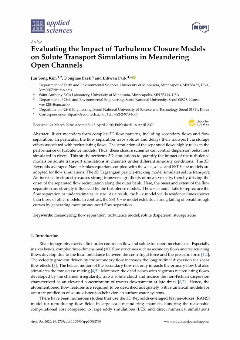
Figure 6 shows that the separated recirculation zones emerge near the outer bank of the bendinlet in high-sinuosity cases of S157 and S190, as shown in Figure 6. Hickin [60] revealed that theonset of the horizontal flow separation occurs at a specific level of the curvature ratio to channelwidth, Rc/W ≤ 2, which is consistent with Rc/W of S157 and S190, as presented in Table 1. Accordingto Figure 6, however, the onset and size of the recirculation zones highly depend on the turbulencemodels. In S157, the k−ω and SST k−ω models adequately reproduce the onset of the recirculatingflows, while the k− ε model fails to simulate the flow separation. In S190, all turbulence models aresuccessful in reproducing the separated recirculating flows. Nevertheless, the k− ε and k−ω modelsunpredict the reattachment length of the flow separation for both S157 and S190 compared to the SSTk−ω model (Figure 6).
Appl. Sci. 2020, 10, 2769 10 of 17
Appl. Sci. 2020, 9, x FOR PEER REVIEW 10 of 18
The high sinuosity causes the transverse gradient of the streamwise velocity biased largely
toward the inner bank. This strong velocity gradient in the transverse direction forms the low-
velocity zones near the outer bank, where it is notable that the negative streamwise velocity (backflow)
is simulated at the bend apex with the SST -k ω model for S190, as shown in Figure 5a. From the
backflow, it is evident that horizontal recirculating flows take place in the vicinity of the outer bank
owing to the adverse pressure gradients associated with the sharp bend curvature. At high sinuosity,
the streamwise velocity structures are substantially influenced by the turbulence models (Figure 5a).
Thus, it can be inferred that the turbulence models may directly affect the recirculating flow
characteristics.
Figure 6 shows that the separated recirculation zones emerge near the outer bank of the bend
inlet in high-sinuosity cases of S157 and S190, as shown in Figure 6. Hickin [60] revealed that the
onset of the horizontal flow separation occurs at a specific level of the curvature ratio to channel
width, / 2c
R W , which is consistent with /c
R W of S157 and S190, as presented in Table 1.
According to Figure 6, however, the onset and size of the recirculation zones highly depend on the
turbulence models. In S157, the -k ω and SST -k ω models adequately reproduce the onset of the
recirculating flows, while the -k ε model fails to simulate the flow separation. In S190, all turbulence
models are successful in reproducing the separated recirculating flows. Nevertheless, the -k ε and
-k ω models unpredict the reattachment length of the flow separation for both S157 and S190
compared to the SST -k ω model (Figure 6).
Figure 6. Streamlines of velocity fields for (a) S157 and (b) S190, simulated with different turbulence
models. RL indicates the reattachment length of recirculation zones.
The influence of the turbulence models on the flow separation is further examined using its
width and velocity magnitude. The transverse distributions of the depth-averaged mean velocity at
the cross-section across the center of the recirculation zones is plotted in Figure 7. With this figure,
the width of the recirculation zones is implicitly estimated by measuring the distance between the
center of the recirculation zone and the wall. Please note that this study assumes the minimum-
velocity point other than the near-wall boundary as the center of the recirculation zone, as illustrated
in Figure 7b. In S136, no flow recirculation is simulated with all turbulence models as the minimum
velocity occurs very near the wall, as shown in Figure 7a. For S157 and S190, the SST -k ω model
reproduces the faster and wider recirculating flows than those of other turbulence models, as
depicted in Figure 7b,c. Particularly in S157, the -k ε model simulates the width of the recirculation
(a)
(b)
LR/W ≈ 1.2
LR/W ≈ 2
LR/W ≈ 0
LR/W ≈ 2 LR/W ≈ 2.7
k-ε k-ω SST
k-ε k-ω SST
LR/W ≈ 3.6
U (m/s)
0.700
0
0.350
0.175
0.525
y
x
Figure 6. Streamlines of velocity fields for (a) S157 and (b) S190, simulated with different turbulencemodels. LR indicates the reattachment length of recirculation zones.
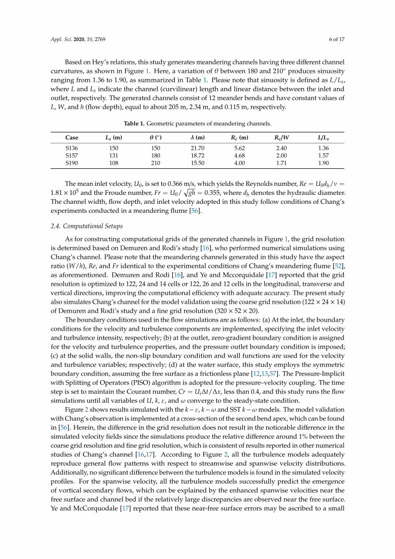
The influence of the turbulence models on the flow separation is further examined using its widthand velocity magnitude. The transverse distributions of the depth-averaged mean velocity at thecross-section across the center of the recirculation zones is plotted in Figure 7. With this figure, thewidth of the recirculation zones is implicitly estimated by measuring the distance between the centerof the recirculation zone and the wall. Please note that this study assumes the minimum-velocity pointother than the near-wall boundary as the center of the recirculation zone, as illustrated in Figure 7b.In S136, no flow recirculation is simulated with all turbulence models as the minimum velocity occursvery near the wall, as shown in Figure 7a. For S157 and S190, the SST k −ω model reproduces thefaster and wider recirculating flows than those of other turbulence models, as depicted in Figure 7b,c.Particularly in S157, the k− ε model simulates the width of the recirculation zone close to zero, whichindicates no occurrence of the flow separation (Figure 7b). These trends are consistent with the findingsfrom Figure 6.
Appl. Sci. 2020, 9, x FOR PEER REVIEW 11 of 18
zone close to zero, which indicates no occurrence of the flow separation (Figure 7b). These trends are
consistent with the findings from Figure 6.
Figure 7. Distributions of depth-averaged mean velocity at the cross-section crossing the center of
recirculation zones for (a) S136, (b) S157, and (c) S190. The insets plot the distributions with the
logarithmic scale on y -axis.
In the meandering channel studied in this work, the extent of the separated flow recirculation
would be critical in quantifying the magnitude of the non-Fickian transport because the larger
recirculation zones trap more solute particles and directly contribute to longer residence times of
solutes. Additionally, the recirculating flow velocity may be significantly related to the trapping
effects. The mass exchange between the main flow zone and the recirculation zone occurs via
turbulent diffusion along the interface between the two different flow regimes, where the turbulent
shear layer develops. Here, the fast recirculating flows suppress the solute diffusion from the
recirculation zone into the main flow zone because of the strong inertial effects, thereby enhancing
the trapping effects. As previously demonstrated, the onset, size, and velocity magnitude of the
recirculating flows are considerably sensitive to the turbulence models. In consequence, it can be
expected that the turbulence models control the non-Fickian transport behaviors simulated in the
meandering channels.
3.3. Solute Transport and Dispersion
For solute transport simulations, 2 × 10⁵ particles are instantaneously injected as a point source
introduced from the center of the inlet cross-section, and the simulated mean velocity and turbulence
fields at the steady state are used as input variables to govern advection and diffusion of the solute
particles, respectively. The time step is set to retain Cr to be unity [7]. The effects of sinuosity on
solute dispersion are first investigated. Figure 8 presents one-dimensional (1D) breakthrough curves
(BTCs) at the channel outlet, simulated with the -k ε , -k ω and SST -k ω models. This figure
indicates probability density functions of particle residence times until they pass the outlet, which
can conventionally be considered as particle residence time distributions. Herein, the probability
density is calculated as the ratio of the number of particles, which pass the outlet at each measurement
interval of 20 s (bin width of Figure 8), to the total particles of 2 × 10⁵ divided by the bin width. As
shown in Figure 8, the longitudinal dispersion increases as sinuosity increases because the higher
sinuosity leads to the larger elongation of the solute spreading in the streamwise direction, honoring
the larger velocity gradients in the transverse direction. This trend is commonly observed in the BTCs
simulated with all turbulence models. Yet, the tail scaling of the BTCs differ according to the
turbulence models, as depicted in Figure 8. The scaling (slope) of the BTC tails is conventionally
considered as a vital factor in quantifying the non-Fickian dispersion [61,62].
(a) (b)
y/W y/W y/W
(c)k-εk-ωSST
0U
/U
The center of
a recirculation zone
Figure 7. Distributions of depth-averaged mean velocity at the cross-section crossing the center ofrecirculation zones for (a) S136, (b) S157, and (c) S190. The insets plot the distributions with thelogarithmic scale on y-axis.
In the meandering channel studied in this work, the extent of the separated flow recirculationwould be critical in quantifying the magnitude of the non-Fickian transport because the largerrecirculation zones trap more solute particles and directly contribute to longer residence times of

Appl. Sci. 2020, 10, 2769 11 of 17
solutes. Additionally, the recirculating flow velocity may be significantly related to the trappingeffects. The mass exchange between the main flow zone and the recirculation zone occurs via turbulentdiffusion along the interface between the two different flow regimes, where the turbulent shear layerdevelops. Here, the fast recirculating flows suppress the solute diffusion from the recirculation zoneinto the main flow zone because of the strong inertial effects, thereby enhancing the trapping effects.As previously demonstrated, the onset, size, and velocity magnitude of the recirculating flows areconsiderably sensitive to the turbulence models. In consequence, it can be expected that the turbulencemodels control the non-Fickian transport behaviors simulated in the meandering channels.
3.3. Solute Transport and Dispersion
For solute transport simulations, 2 × 10⁵ particles are instantaneously injected as a point sourceintroduced from the center of the inlet cross-section, and the simulated mean velocity and turbulencefields at the steady state are used as input variables to govern advection and diffusion of the soluteparticles, respectively. The time step is set to retain Cr to be unity [7]. The effects of sinuosity on solutedispersion are first investigated. Figure 8 presents one-dimensional (1D) breakthrough curves (BTCs) atthe channel outlet, simulated with the k− ε, k−ω and SST k−ωmodels. This figure indicates probabilitydensity functions of particle residence times until they pass the outlet, which can conventionally beconsidered as particle residence time distributions. Herein, the probability density is calculated asthe ratio of the number of particles, which pass the outlet at each measurement interval of 20 s (binwidth of Figure 8), to the total particles of 2 × 10⁵ divided by the bin width. As shown in Figure 8,the longitudinal dispersion increases as sinuosity increases because the higher sinuosity leads to thelarger elongation of the solute spreading in the streamwise direction, honoring the larger velocitygradients in the transverse direction. This trend is commonly observed in the BTCs simulated withall turbulence models. Yet, the tail scaling of the BTCs differ according to the turbulence models, asdepicted in Figure 8. The scaling (slope) of the BTC tails is conventionally considered as a vital factorin quantifying the non-Fickian dispersion [61,62].Appl. Sci. 2020, 9, x FOR PEER REVIEW 12 of 18
Figure 8. 1D breakthrough curves of S136, S157, and S190, in which particle residence times are
measured at the channel outlet, simulated with (a) the -k ε model, (b) the -k ω model, and (c) the
SST -k ω model.
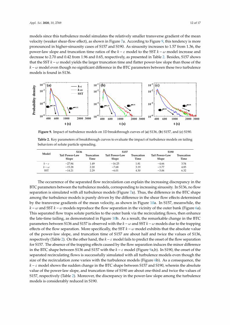
Figure 9 shows the impact of the turbulence models on the BTC tailing with a variation of
channel sinuosity and demonstrates that the -k ω and SST -k ωmodels exhibit the heavier-tailed
BTCs than those of the -k ε model. To quantify this disparity among the turbulence models, this
study estimates the tail power-law slope and the truncation time, which are measures of the non-
Fickian dispersion [41,61,62]. Here, the truncation time is defined as the ratio of the maximum
residence time to the peak concentration time [57], and the power-law slope is calculated using the
least-squares regression. Please note that the flatter power-law slope (smaller its absolute value) and
larger truncation time characterize the stronger non-Fickian dispersion with the heavier BTC tailing.
The power-law slope and truncation time for all simulation cases are summarized in Table 2. In S136,
the -k ε model exhibits the steeper power-law slope and smaller truncation time than those of other
turbulence models since this turbulence model simulates the relatively smaller transverse gradient
of the mean velocity (weaker shear-flow effect), as shown in Figure 7a. According to Figure 9, this
tendency is more pronounced in higher-sinuosity cases of S157 and S190. As sinuosity increases to
1.57 from 1.36, the power-law slope and truncation time ratios of the -k ε model to the SST -k ω
model increase and decrease to 2.70 and 0.42 from 1.96 and 0.65, respectively, as presented in Table
2. Besides, S157 shows that the SST -k ω model yields the larger truncation time and flatter power-
law slope than those of the -k ω model even though no significant difference in the BTC parameters
between these two turbulence models is found in S136.
Figure 9. Impact of turbulence models on 1D breakthrough curves of (a) S136, (b) S157, and (c) S190.
Pro
ba
bil
ity
den
sity
t (s)
(a) (b) (c)
t (s) t (s)
27.84t
4.66t
15.28t
3.77t
14.21t
3.06t
Pro
ba
bil
ity
den
sity
t (s) t (s) t (s)
(a) (b) (c)k-ε
k-ω
SST
27.84t
4.66t
14.21t
3.06t16.25
t
6.01t
Figure 8. 1D breakthrough curves of S136, S157, and S190, in which particle residence times aremeasured at the channel outlet, simulated with (a) the k− ε model, (b) the k−ω model, and (c) the SSTk−ω model.
Figure 9 shows the impact of the turbulence models on the BTC tailing with a variation of channelsinuosity and demonstrates that the k − ω and SST k − ω models exhibit the heavier-tailed BTCsthan those of the k − ε model. To quantify this disparity among the turbulence models, this studyestimates the tail power-law slope and the truncation time, which are measures of the non-Fickiandispersion [41,61,62]. Here, the truncation time is defined as the ratio of the maximum residence timeto the peak concentration time [57], and the power-law slope is calculated using the least-squaresregression. Please note that the flatter power-law slope (smaller its absolute value) and larger truncationtime characterize the stronger non-Fickian dispersion with the heavier BTC tailing. The power-lawslope and truncation time for all simulation cases are summarized in Table 2. In S136, the k− ε modelexhibits the steeper power-law slope and smaller truncation time than those of other turbulence
Appl. Sci. 2020, 10, 2769 12 of 17
models since this turbulence model simulates the relatively smaller transverse gradient of the meanvelocity (weaker shear-flow effect), as shown in Figure 7a. According to Figure 9, this tendency is morepronounced in higher-sinuosity cases of S157 and S190. As sinuosity increases to 1.57 from 1.36, thepower-law slope and truncation time ratios of the k − ε model to the SST k −ω model increase anddecrease to 2.70 and 0.42 from 1.96 and 0.65, respectively, as presented in Table 2. Besides, S157 showsthat the SST k−ω model yields the larger truncation time and flatter power-law slope than those of thek−ωmodel even though no significant difference in the BTC parameters between these two turbulencemodels is found in S136.
Appl. Sci. 2020, 9, x FOR PEER REVIEW 12 of 18
Figure 8. 1D breakthrough curves of S136, S157, and S190, in which particle residence times are
measured at the channel outlet, simulated with (a) the -k ε model, (b) the -k ω model, and (c) the
SST -k ω model.
Figure 9 shows the impact of the turbulence models on the BTC tailing with a variation of
channel sinuosity and demonstrates that the -k ω and SST -k ωmodels exhibit the heavier-tailed
BTCs than those of the -k ε model. To quantify this disparity among the turbulence models, this
study estimates the tail power-law slope and the truncation time, which are measures of the non-
Fickian dispersion [41,61,62]. Here, the truncation time is defined as the ratio of the maximum
residence time to the peak concentration time [57], and the power-law slope is calculated using the
least-squares regression. Please note that the flatter power-law slope (smaller its absolute value) and
larger truncation time characterize the stronger non-Fickian dispersion with the heavier BTC tailing.
The power-law slope and truncation time for all simulation cases are summarized in Table 2. In S136,
the -k ε model exhibits the steeper power-law slope and smaller truncation time than those of other
turbulence models since this turbulence model simulates the relatively smaller transverse gradient
of the mean velocity (weaker shear-flow effect), as shown in Figure 7a. According to Figure 9, this
tendency is more pronounced in higher-sinuosity cases of S157 and S190. As sinuosity increases to
1.57 from 1.36, the power-law slope and truncation time ratios of the -k ε model to the SST -k ω
model increase and decrease to 2.70 and 0.42 from 1.96 and 0.65, respectively, as presented in Table
2. Besides, S157 shows that the SST -k ω model yields the larger truncation time and flatter power-
law slope than those of the -k ω model even though no significant difference in the BTC parameters
between these two turbulence models is found in S136.
Figure 9. Impact of turbulence models on 1D breakthrough curves of (a) S136, (b) S157, and (c) S190.
Pro
ba
bil
ity
den
sity
t (s)
(a) (b) (c)
t (s) t (s)
27.84t
4.66t
15.28t
3.77t
14.21t
3.06t
Pro
ba
bil
ity
den
sity
t (s) t (s) t (s)
(a) (b) (c)k-ε
k-ω
SST
27.84t
4.66t
14.21t
3.06t16.25
t
6.01t
Figure 9. Impact of turbulence models on 1D breakthrough curves of (a) S136, (b) S157, and (c) S190.
Table 2. Key parameters of breakthrough curves to evaluate the impact of turbulence models on tailingbehaviors of solute particle spreading.
ModelS136 S157 S190
Tail Power-LawSlope
TruncationTime
Tail Power-LawSlope
TruncationTime
Tail Power-LawSlope
TruncationTime
k− ε −27.84 1.49 −16.25 1.81 −4.66 3.54k−ω −15.28 2.20 −7.68 3.19 −3.77 4.85SST −14.21 2.29 −6.01 4.30 −3.06 6.32
The occurrence of the separated flow recirculation can explain the increasing discrepancy in theBTC parameters between the turbulence models, corresponding to increasing sinuosity. In S136, no flowseparation is simulated with all turbulence models (Figure 7a). Thus, the difference in the BTC shapeamong the turbulence models is purely driven by the difference in the shear flow effects determinedby the transverse gradients of the mean velocity, as shown in Figure 10a. In S157, meanwhile, thek−ω and SST k−ω models reproduce the flow separation in the vicinity of the outer bank (Figure 6a).This separated flow traps solute particles to the outer bank via the recirculating flows, then enhancethe late-time tailing, as demonstrated in Figure 10b. As a result, the remarkable change in the BTCparameters between S136 and S157 is observed with the k−ω and SST k−ωmodels due to the trappingeffects of the flow separation. More specifically, the SST k−ω model exhibits that the absolute valueof the power-law slope, and truncation time of S157 are about half and twice the values of S136,respectively (Table 2). On the other hand, the k− εmodel fails to predict the onset of the flow separationfor S157. The absence of the trapping effects caused by the flow separation induces the minor differencein the BTC shape between S136 and S157 with the k− ε model (Figure 9a,b). In S190, the onset of theseparated recirculating flows is successfully simulated with all turbulence models even though thesize of the recirculation zone varies with the turbulence models (Figure 6b). As a consequence, thek− ε model shows the sudden change in the BTC shape between S157 and S190, wherein the absolutevalue of the power-law slope, and truncation time of S190 are about one-third and twice the values ofS157, respectively (Table 2). Moreover, the discrepancy in the power-law slope among the turbulencemodels is considerably reduced in S190.
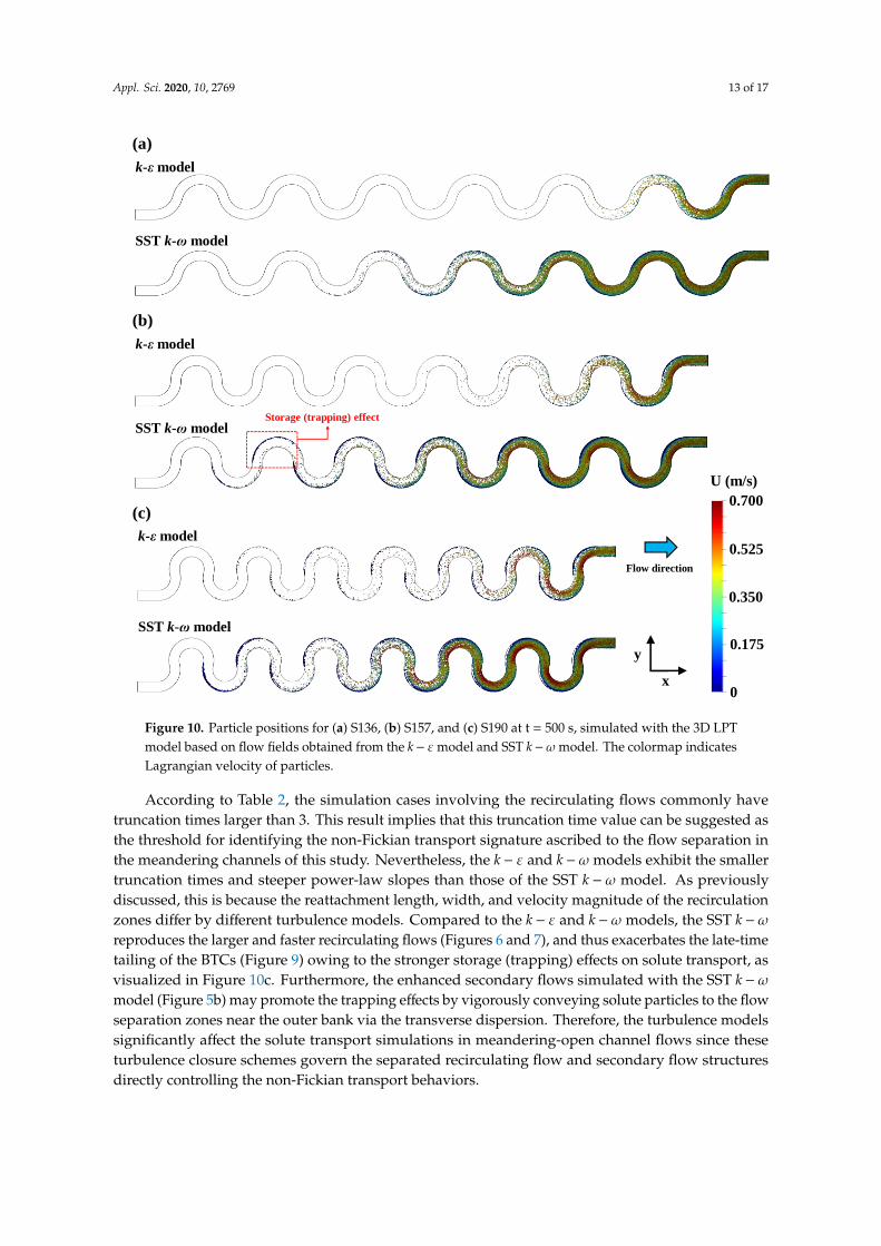
Appl. Sci. 2020, 10, 2769 13 of 17Appl. Sci. 2020, 9, x FOR PEER REVIEW 14 of 18
Figure 10. Particle positions for (a) S136, (b) S157, and (c) S190 at t = 500 s, simulated with the 3D LPT
model based on flow fields obtained from the -k ε model and SST -k ω model. The colormap
indicates Lagrangian velocity of particles.
According to Table 2, the simulation cases involving the recirculating flows commonly have
truncation times larger than 3. This result implies that this truncation time value can be suggested as
the threshold for identifying the non-Fickian transport signature ascribed to the flow separation in
the meandering channels of this study. Nevertheless, the -k ε and -k ωmodels exhibit the smaller
truncation times and steeper power-law slopes than those of the SST -k ω model. As previously
discussed, this is because the reattachment length, width, and velocity magnitude of the recirculation
zones differ by different turbulence models. Compared to the -k ε and -k ωmodels, the SST -k ω
reproduces the larger and faster recirculating flows (Figures 6 and 7), and thus exacerbates the late-
time tailing of the BTCs (Figure 9) owing to the stronger storage (trapping) effects on solute transport,
as visualized in Figure 10c. Furthermore, the enhanced secondary flows simulated with the SST -k ω
model (Figure 5b) may promote the trapping effects by vigorously conveying solute particles to the
flow separation zones near the outer bank via the transverse dispersion. Therefore, the turbulence
models significantly affect the solute transport simulations in meandering-open channel flows since
these turbulence closure schemes govern the separated recirculating flow and secondary flow
structures directly controlling the non-Fickian transport behaviors.
4. Conclusions
This study quantified the influence of turbulence closure models in simulating curvature-driven
flow separation and resulting non-Fickian mixing behaviors in meandering open channels across a
k-ε model
SST k-ω model
U (m/s)
0.700
0
0.350
0.175
0.525k-ε model
SST k-ω model
(b)
(c)
k-ε model
SST k-ω model
(a)
Flow direction
y
x
Storage (trapping) effect
Figure 10. Particle positions for (a) S136, (b) S157, and (c) S190 at t = 500 s, simulated with the 3D LPTmodel based on flow fields obtained from the k− εmodel and SST k−ωmodel. The colormap indicatesLagrangian velocity of particles.
According to Table 2, the simulation cases involving the recirculating flows commonly havetruncation times larger than 3. This result implies that this truncation time value can be suggested asthe threshold for identifying the non-Fickian transport signature ascribed to the flow separation inthe meandering channels of this study. Nevertheless, the k− ε and k−ω models exhibit the smallertruncation times and steeper power-law slopes than those of the SST k −ω model. As previouslydiscussed, this is because the reattachment length, width, and velocity magnitude of the recirculationzones differ by different turbulence models. Compared to the k − ε and k −ω models, the SST k −ωreproduces the larger and faster recirculating flows (Figures 6 and 7), and thus exacerbates the late-timetailing of the BTCs (Figure 9) owing to the stronger storage (trapping) effects on solute transport, asvisualized in Figure 10c. Furthermore, the enhanced secondary flows simulated with the SST k −ωmodel (Figure 5b) may promote the trapping effects by vigorously conveying solute particles to the flowseparation zones near the outer bank via the transverse dispersion. Therefore, the turbulence modelssignificantly affect the solute transport simulations in meandering-open channel flows since theseturbulence closure schemes govern the separated recirculating flow and secondary flow structuresdirectly controlling the non-Fickian transport behaviors.

Appl. Sci. 2020, 10, 2769 14 of 17
4. Conclusions
This study quantified the influence of turbulence closure models in simulating curvature-drivenflow separation and resulting non-Fickian mixing behaviors in meandering open channels across awide range of sinuosity. To achieve this task, the 3D RANS equations integrated with k− ε, k−ω andSST k−ω turbulence models were used for flow simulations, and the 3D LPT model was adopted forsolute transport simulations. The major findings from this work can be summarized as:
• The strong transverse gradients of mean velocity simulated with increasing sinuosity induce theflow separation along the outer bank for channel sinuosity 1.57 and 1.90 because of the adversepressure gradients. The size of the flow separation increases as sinuosity increases.
• The onset and size of the flow separation are significantly affected by the turbulence models.Notably, the k − ε model fails to predict the emergence of the flow separation or unpredicts itsreattachment length and width by underestimating the velocity gradients.
• The flow separation with vigorous recirculating flows acts as a storage (trapping) zone ofsolute particles, and the trapping effects increase solute residence times. Here, the k − ε modelunderestimates the power-law tailing of BTCs since it undervalues the effects of the separatedflow recirculation compared to the other turbulence models.
• The SST k −ω model yields heavier-tailed BTCs characterized by flatter power-law slopes andlarger truncation times as it reproduces larger and faster recirculating flows than the k − ε andk−ω models.
Consequently, the present work elucidated that the turbulence models substantially impact the3D solute transport simulations since these turbulence closure schemes determine the onset and extentof the separated flow recirculation identified as the surface storage zones. Even if the 3D model iseffective in explicitly understanding the interaction between solute dispersion and hydrodynamiceffects, this approach may not be appropriate for water quality management in rivers and streamsbecause of the high computational demand. Therefore, the next stage of this study will parameterizethe transient storage model, which is the 1D upscaled model extensively used for simulating thenon-Fickian transport in rivers and streams [63], using the simulation results of this work and predictthe heavy-tailed BTCs induced by the meander-driven flow separation.
Author Contributions: Conceptualization and visualization, J.S.K.; Simulations, J.S.K. and D.B.; writing—originaldraft preparation, J.S.K. and I.P.; writing—review and editing, J.S.K. and I.P.; funding acquisition, I.P. All authorshave read and agreed to the published version of the manuscript.
Funding: This study was supported by the Research Program funded by the SeoulTech (Seoul National Universityof Science and Technology).
Conflicts of Interest: The authors declare no conflict of interest.
References
1. Johannesson, H.; Parker, G. Secondary flow in mildly sinuous channel. J. Hydraul. Eng. 1989, 115, 289–308.[CrossRef]
2. Blanckaert, K.; de Vriend, H.J. Nonlinear modeling of mean flow redistribution in curved open channels.Water Resour. Res. 2003, 39. [CrossRef]
3. Marion, A.; Zaramella, M. Effects of velocity gradients and secondary flow on the dispersion of solutes in ameandering channel. J. Hydraul. Eng. 2006, 132, 1295–1302. [CrossRef]
4. Boxall, J.B.; Guymer, I. Analysis and prediction of transverse mixing coefficients in natural channels. J.Hydraul. Eng. 2003, 129, 129–139. [CrossRef]
5. Baek, K.O.; Seo, I.W.; Jeong, S.J. Evaluation of dispersion coefficients in meandering channels from transienttracer tests. J. Hydraul. Eng. 2006, 132, 1021–1032. [CrossRef]
6. Davis, P.M.; Atkinson, T.C.; Wigley, T.M.L. Longitudinal dispersion in natural channels: 2. The roles of shearflow dispersion and dead zones in the River Severn, UK. Hydrol. Earth Syst. Sci. 2000, 4, 355–371. [CrossRef]

Appl. Sci. 2020, 10, 2769 15 of 17
7. Park, I.; Seo, I.W. Modeling non-Fickian pollutant mixing in open channel flows using two-dimensionalparticle dispersion model. Adv. Water Resour. 2018, 111, 105–120. [CrossRef]
8. Rameshwaran, P.; Nade, P.S. Three-dimensional modelling of free surface variation in a meandering channel.J. Hydraul. Res. 2004, 42, 603–615. [CrossRef]
9. Wormleaton, P.R.; Ewunetu, M. Three-dimensional k-ε numerical modelling of overbank flow in a mobilebed meandering channel with floodplains of different depth, roughness and planform. J. Hydraul. Res. 2006,44, 18–32. [CrossRef]
10. Fischer-Antze, T.; Ruther, N.; Olsen, N.R.B.; Gutknecht, D. Three-dimensional (3D) modeling of non-uniformsediment transport in a channel bend with unsteady flow. J. Hydraul. Res. 2009, 47, 670–675. [CrossRef]
11. Rüther, N.; Olsen, N.R.B. Three-dimensional modeling of sediment transport in a narrow 90◦ channel bend.J. Hydraul. Eng. 2005, 131, 917–920. [CrossRef]
12. Stoesser, T.; Ruether, N.; Olsen, N.R.B. Calculation of primary and secondary flow and boundary shearstresses in a meandering channel. Adv. Water Resour. 2010, 33, 158–170. [CrossRef]
13. Van Balen, W.; Blanckaert, K.; Uijttewaal, W.S.J. Analysis of the role of turbulence in curved open-channelflow at different water depths by means of experiments, LES and RANS. J. Turbul. 2010, 11, 1–34. [CrossRef]
14. Farhadi, A.; Sindelar, C.; Tritthart, M.; Glas, M.; Blanckaert, K.; Habersack, H. An investigation on the outerbank cell of secondary flow in channel bends. J. Hydro-Environ. Res. 2018, 18, 1–11. [CrossRef]
15. Russell, P.; Vennell, R. High resolution observations of an outer-bank cell of secondary circulation in a naturalriver bend. J. Hydraul. Res. 2019, 145, 04019012. [CrossRef]
16. Demuren, A.O.; Rodi, W. Calculation of flow and pollutant dispersion in meandering channels. J. Fluid Mech.1986, 172, 63–92. [CrossRef]
17. Ye, J.; McCorquodale, J.A. Simulation of curved open channel flows by 3D hydrodynamic model. J. Hydraul.Eng. 1998, 124, 687–698. [CrossRef]
18. Ferguson, R.I.; Parsons, D.R.; Lane, S.N.; Hardy, R.J. Flow in meander bends with recirculation at the innerbank. Water Resour. Res. 2003, 39. [CrossRef]
19. Abad, J.D.; Frias, C.E.; Buscaglia, G.C.; Garcia, M.H. Modulation of the flow structure by progressivebedforms in the Kinoshita meandering channel. Earth Surf. Process. Landf. 2013, 38, 1612–1622. [CrossRef]
20. Rameshwaran, P.; Naden, P.; Wilson, C.A.; Malki, R.; Shukla, D.R.; Shiono, K. Inter-comparison and validationof computational fluid dynamics codes in two-stage meandering channel flows. Appl. Math. Model. 2013, 37,8652–8672. [CrossRef]
21. Argyropoulos, C.D.; Markatos, N.C. Recent advances on the numerical modelling of turbulent flows. Appl.Math. Model. 2015, 39, 693–732. [CrossRef]
22. Wilcox, D.C. Formulation of the k-ω turbulence model revisited. AIAAJ J. 2008, 46, 2823–2838. [CrossRef]23. El-Behery, S.M.; Hamed, M.H. A comparative study of turbulence models performance for separating flow
in a planar asymmetric diffuser. Comput. Fluids 2011, 44, 248–257. [CrossRef]24. Khosronejad, A.; Rennie, C.D.; Salehi Neyshabouri, S.A.A.; Townsend, R.D. 3D numerical modeling of flow
and sediment transport in laboratory channel bends. J. Hydraul. Eng. 2007, 133, 1123–1134. [CrossRef]25. Menter, F.R. Two-equation eddy-viscosity turbulence models for engineering applications. AIAA J. 1994, 32,
1598–1605. [CrossRef]26. Sparrow, E.M.; Abraham, J.P.; Minkowycz, W.J. Flow separation in a diverging conical duct: Effect of
Reynolds number and divergence angle. Int. J. Heat Mass Transf. 2009, 52, 3079–3083. [CrossRef]27. Luo, H.; Fytanidis, D.K.; Schmidt, A.R.; García, M.H. Comparative 1D and 3D numerical investigation of
open-channel junction flows and energy losses. Adv. Water Resour. 2018, 117, 120–139. [CrossRef]28. Nguyen, T.H.T.; Ahn, J.; Park, S.W. Numerical and physical investigation of the performance of turbulence
modeling schemes around a scour hole downstream of a fixed bed protection. Water 2018, 10, 103. [CrossRef]29. Khosronejad, A.; Hansen, A.T.; Kozarek, J.L.; Guentzel, K.; Hondzo, M.; Guala, M.; Wilcock, P.R.; Finlay, J.C.
Large eddy simulation of turbulence and solute transport in a forested headwater stream. J. Geophys. Res.Earth Surf. 2016, 121, 146–167. [CrossRef]
30. Kim, J.S.; Baek, D.; Seo, I.W.; Shin, J. Retrieving shallow stream bathymetry from UAV-assisted RGB imageryusing a geospatial regression method. Geomorphology 2019, 341, 102–114. [CrossRef]
31. Blanckaert, K. Topographic steering, flow recirculation, velocity redistribution, and bed topography in sharpmeander bends. Water Resour. Res. 2010, 46. [CrossRef]

Appl. Sci. 2020, 10, 2769 16 of 17
32. Blanckaert, K. Hydrodynamic processes in sharp meander bends and their morphological implications. J.Geophys. Res. Earth Surf. 2011, 116. [CrossRef]
33. Blanckaert, K.; Kleinhans, M.G.; McLelland, S.J.; Uijttewaal, W.S.; Murphy, B.J.; van de Kruijs, A.; Parsons, D.R.;Chen, Q. Flow separation at the inner (convex) and outer (concave) banks of constant-width and wideningopen-channel bends. Earth Surf. Process. Landf. 2013, 38, 696–716. [CrossRef]
34. Jackson, T.R.; Haggerty, R.; Apte, S.V.; Coleman, A.; Drost, K.J. Defining and measuring the mean residencetime of lateral surface transient storage zones in small streams. Water Resour. Res. 2012, 48. [CrossRef]
35. Sandoval, J.; Mignot, E.; Mao, L.; Pastén, P.; Bolster, D.; Escauriaza, C. Field numerical investigation oftransport mechanisms in a surface storage zone. J. Geophys. Res. Earth Surf. 2019, 124, 938–959. [CrossRef]
36. Wilson, C.A.M.E.; Guymer, I.; Boxall, J.B.; Olsen, N.R.B. Three-dimensional numerical simulation of solutetransport in a meandering self-formed river channel. J. Hydraul. Res. 2007, 45, 610–616. [CrossRef]
37. Zhang, M.L.; Li, C.W.; Shen, Y.M. A 3D non-linear k-ε turbulent model for prediction of flow and masstransport in channel with vegetation. Appl. Math. Model. 2010, 34, 1021–1031. [CrossRef]
38. Liu, X.; García, M.H. Three-dimensional numerical model with free water surface and mesh deformation forlocal sediment scour. J. Waterw. Port Coast. Ocean Eng. 2008, 134, 203–217. [CrossRef]
39. Bayon-Barrachina, A.; Lopez-Jimenez, P.A. Numerical analysis of hydraulic jumps using OpenFOAM. J.Hydroinform. 2015, 17, 662–678. [CrossRef]
40. Bayon, A.; Valero, D.; García-Bartual, R.; Vallés-Morán, F.J. Performance assessment of OpenFOAM andFLOW-3D in the numerical modeling of a low Reynolds number hydraulic jump. Environ. Model. Softw.2016, 80, 322–335. [CrossRef]
41. Hromadka, T.V., II; Rao, P. Examination of computational precision versus modeling complexity for openchannel flow with hydraulic jump. J. Water Resour. Prot. 2019, 11, 1233–1244.
42. Wang, Y.; Politano, M.; Laughery, R.; Weber, L. Model development in OpenFOAM to predict spillway jetregimes. J. Appl. Water Eng. Res. 2015, 3, 80–94. [CrossRef]
43. Duguay, J.M.; Lacey, R.W.J.; Gaucher, J. A case study of a pool and weir fishway modeled with OpenFOAMand FLOW-3D. Ecol. Model. 2017, 103, 31–42. [CrossRef]
44. Bayon, A.; Toro, J.P.; Bombardelli, F.A.; Matos, J.; López-Jiménez, P.A. Influence of VOF technique, turbulencemodel and discretization scheme on the numerical simulation of the non-aerated, skimming flow in steppedspillways. J. Hydro-Environ. Res. 2018, 19, 137–149. [CrossRef]
45. Kim, J.S.; Kang, P.K. Anomalous transport through free-flow-porous media interface: Pore-scale simulationand predictive modeling. Adv. Water Resour. 2020, 135, 103467. [CrossRef]
46. Jones, W.P.; Launder, B.E. The prediction of laminarization with a two-equation model of turbulence. Int.Heat Mass Transfer. 1972, 15, 301–314. [CrossRef]
47. Pope, S.B. Turbulent Flows; Cambridge University Press: Cambridge, UK, 2000; pp. 373–384.48. Zeng, J.; Constantinescu, G.; Weber, L. A 3D non-hydrostatic model to predict flow and sediment transport
in loose-bed channel bends. J. Hydraul. Res. 2008, 46, 56–372. [CrossRef]49. Kang, S.; Lightbody, A.; Hill, C.; Sotiropoulos, F. High-resolution numerical simulation of turbulence in
natural waterways. Adv. Water Resour. 2011, 34, 98–113. [CrossRef]50. Kang, S.; Sotiropoulos, F. Numerical modeling of 3D turbulent free surface flow in natural waterways. Adv.
Water Resour. 2012, 40, 23–36. [CrossRef]51. Gosman, A.D.; Loannides, E. Aspects of computer simulation of liquid-fueled combustors. J. Energy 1983, 7,
482–490. [CrossRef]52. Shams, M.; Ahmadi, G.; Smith, D.H. Computational modeling of flow and sediment transport and deposition
in meandering rivers. Adv. Water Resour. 2002, 25, 689–699. [CrossRef]53. Dehbi, A. Turbulent particle dispersion in arbitrary wall-bounded geometries: A coupled
CFD-Langevin-equation based approach. Int. J. Multiph. Flow 2008, 34, 819–828. [CrossRef]54. Rybalko, M.; Loth, E.; Lankford, D.A. Lagrangian particle random walk model for hybrid RANS/LES
turbulent flows. Powder Technol. 2012, 221, 105–113. [CrossRef]55. Hey, R.D. Geometry of river meanders. Nature 1976, 262, 482. [CrossRef]56. Chang, Y.C. Lateral mixing in meandering channels. In River Meandering; ASCE: Reston, VA, USA, 1971;
pp. 598–610.

Appl. Sci. 2020, 10, 2769 17 of 17
57. Hodskinson, A.; Ferguson, R.I. Numerical modelling of separated flow in river bends: Model testing andexperimental investigation of geometric controls on the extent of flow separation at the concave bank. Hydrol.Process. 1998, 12, 1323–1338. [CrossRef]
58. Vinuesa, R.; Schlatter, P.; Nagib, H.M. Secondary flow in turbulent ducts with increasing aspect ratio. Phys.Rev. Fluids 2018, 3, 054606. [CrossRef]
59. Abad, J.D.; Garcia, M.H. Experiments in a high-amplitude Kinoshita meandering channel: 1. Implicationsooi:f bend orientation on mean and turbulent flow structure. Water Resour. Res. 2009, 45. [CrossRef]
60. Hickin, E.J. Mean flow structure in meanders of the Squamish River, British Columbia. Can. J. Earth Sci.1978, 15, 1833–1849. [CrossRef]
61. Aubeneau, A.F.; Hanrahan, B.; Bolster, D.; Tank, J.L. Substrate size and heterogeneity control anomaloustransport in small streams. Geophys. Res. Lett. 2014, 41, 8335–8341. [CrossRef]
62. Drummond, J.D.; Covino, T.P.; Aubeneau, A.F.; Leong, D.; Patil, S.; Schumer, R.; Packman, A.I. Effects ofsolute breakthrough curve tail truncation on residence time estimates: A synthesis of solute tracer injectionstudies. J. Geophys. Res. Biogeosci. 2012, 117. [CrossRef]
63. Runkel, R.L.; Chapra, S.C. An efficient numerical solution of the transient storage equations for solutetransport in small streams. Water Resour. Res. 1993, 29, 211–215. [CrossRef]
© 2020 by the authors. Licensee MDPI, Basel, Switzerland. This article is an open accessarticle distributed under the terms and conditions of the Creative Commons Attribution(CC BY) license (http://creativecommons.org/licenses/by/4.0/).


![Modeling the influence of wave-enhanced turbulence in a ... · [6] The efficacy of using the k-w turbulence closure model for simulating the wave enhanced surface layer was explored](https://img.dokumen.tips/doc/110x75/5f2249b02013846f724ac9c1/modeling-the-influence-of-wave-enhanced-turbulence-in-a-6-the-efficacy-of.jpg)