Embed Size (px)
Citation preview

IZA DP No. 2041
Evaluating the German "Mini-Job" ReformUsing a True Natural Experiment
Marco CaliendoKatharina Wrohlich
DI
SC
US
SI
ON
PA
PE
R S
ER
IE
S
Forschungsinstitutzur Zukunft der ArbeitInstitute for the Studyof Labor
March 2006

Evaluating the German “Mini-Job” Reform
Using a True Natural Experiment
Marco Caliendo DIW Berlin, IAB Nuremberg
and IZA Bonn
Katharina Wrohlich DIW Berlin and IZA Bonn
Discussion Paper No. 2041
March 2006
IZA
P.O. Box 7240 53072 Bonn
Germany
Phone: +49-228-3894-0 Fax: +49-228-3894-180
Email: [email protected]
Any opinions expressed here are those of the author(s) and not those of the institute. Research disseminated by IZA may include views on policy, but the institute itself takes no institutional policy positions. The Institute for the Study of Labor (IZA) in Bonn is a local and virtual international research center and a place of communication between science, politics and business. IZA is an independent nonprofit company supported by Deutsche Post World Net. The center is associated with the University of Bonn and offers a stimulating research environment through its research networks, research support, and visitors and doctoral programs. IZA engages in (i) original and internationally competitive research in all fields of labor economics, (ii) development of policy concepts, and (iii) dissemination of research results and concepts to the interested public. IZA Discussion Papers often represent preliminary work and are circulated to encourage discussion. Citation of such a paper should account for its provisional character. A revised version may be available directly from the author.

IZA Discussion Paper No. 2041 March 2006
ABSTRACT
Evaluating the German “Mini-Job” Reform Using a True Natural Experiment*
Increasing work incentives for people with low incomes is a common topic in the policy debate across European countries. The “Mini-Job” reform in Germany – introduced on April 1, 2003 – can be seen in line with these policies, exempting labour income below a certain threshold from taxes and employees’ social security contributions. We carry out an ex-post evaluation to identify the short-run effects of this reform. Our identification strategy uses an exogenous variation in the interview months in the German Socio-Economic Panel, that allows us to distinguish groups that are (or are not) affected by the reform. To account for seasonal effects we additionally use a difference-in-differences strategy. The results show that the short-run effects of the reform are limited. We find no significant short-run effects for marginal employment. However, there is evidence that single men who are already employed react immediately and increase secondary job holding. JEL Classification: C25, H31, J68 Keywords: evaluation, natural experiment, difference-in-differences, marginal employment Corresponding author: Marco Caliendo Department of Public Economics DIW Berlin Königin-Luise-Str. 5 14195 Berlin Germany Email: [email protected]
* The authors thank Peter Haan, Benjamin Price, Jürgen Schupp, Viktor Steiner, Arne Uhlendorff and Johannes Ziemendorff as well as seminar participants at DIW for valuable comments. All remaining errors are our own. Financial support of the German Science Foundation (DFG) under the research program “Flexibilisierungspotenziale bei heterogenen Arbeitsmärkten” (project STE 681/5-1) is gratefully acknowledged.

1 Introduction
As a response to persistently high unemployment rates, especially of low-skilled people,
wage subsidies have been intensively discussed in European countries. Following the
example of the Earned Income Tax Credit (EITC) introduced in the 70s in the US
(see, e.g., Scholz, 1996), several European countries have introduced in-work benefits,
tax credits, or subsidies to social security contributions (SSC) for working individuals.
Examples are the Working Family Tax Credit (WFTC) in the UK (see, e.g., Blundell,
Duncan, McCrae, and Meghir, 2000) and the French Prime Pour l’Emploi (see, e.g.,
Stancanelli, 2005).1 The “Mini-Job” reform introduced in Germany in 2003 can also
be seen in line with these policies. The main objective of this reform is to provide
positive work incentives for people with low earnings potential by subsidising social
security contributions. The government expected to achieve that goal by exempting
labour income up to 400 euros from employees’ SSC and introducing a degressive
subsidy for earnings between 401 and 800 euro. To be specific, this reform included
three major changes from pre-reform regulations. First, the maximum amount for
earnings exempted from SSC was increased from 325 to 400 euros. Jobs with earnings
less than this threshold are called mini-jobs. Second, the previous maximum hours
restrictions (15 hours per week) was abolished. Third, income up to 400 euros per
month from a mini-job hold as a secondary job is now exempted from SSC and income
tax.2
The theoretically-expected employment effects of wage subsidies depend on the
design of the policy instrument and on various other institutional and economic factors
(see, e.g., Blundell, 2000, or Moffit, 2003). The expectation of unambiguously positive
effects on labour force participation is based on two conditions. First, the subsidies
have to be targeted at individual income rather than household income, and second,
the reform has to change the incentives to take up work for recipients of unemployment
benefits or other social transfers. The subsidies under the German “Mini-Job” reform
are indeed targeted at the individual level; however, the budget constraint for recipients
of social transfers hardly changes due to strict withdrawal of earnings, as is shown in
Steiner and Wrohlich (2005).
Theoretical predictions about the hours worked, on the other hand, are not so
1For a detailed overview of recent European “Making Work Pay” policy reforms, see Orsini (2006).2See Steiner and Wrohlich (2005) for a more detailed description of the reform.
2

straightforward: for individuals with earnings within the subsidised range it might
be optimal to increase working hours (if the substitution effect dominates the income
effect), whereas for individuals with earnings slightly above 400 euros, it might be
profitable to reduce working hours under the subsidy.3 The total effect on working
hours for the population will therefore depend on the distribution of households along
the working-hours/income distribution and thus has to be evaluated empirically.
A series of papers has estimated the effects of the 2003 “Mini-Job” reform based
on ex-ante simulations with behavioural microsimulation models. They suggest only
very moderate participation effects and even negative effects on working hours.4 This
is in strong contrast to numbers published by official statistics suggesting an additional
number of 930,000 jobs created already one month after introduction of the reform.5
Hence, an ex-post evaluation is called for. This is an especially difficult task here,
since from 2004 onwards various other legal changes have been introduced which might
affect labour supply decisions of individuals. Therefore it should be obvious that a
comparison of the mini-jobs realised in 2004 with pre-reform numbers will not reveal
the true effect of the reform. Furthermore, in contrast to other evaluation studies
of labour market policies, the distinction between control and treatment groups is
not initially clear, since the reform is relevant for the whole population. A thorough
evaluation has to take these points into consideration and should be based on a credible
identification strategy. We will do so by using the exogenous variation in the interview
date of the German Socio-Economic Panel (SOEP). The interviews are conducted
between January and October in each year. Since the reform was introduced on April
1, 2003, we observe some people who are interviewed before the reform and others
interviewed after the new legislation was implemented. This allows us to estimate
the immediate short-run effect of the reform. To account for seasonal variation, we
additionally use a difference-in-differences approach.
We will explain our identification strategy in more detail in Section 2, where we
will also describe the data used for the analysis. Section 3 contains the estimation
results, before Section 4 concludes.
3The same holds for people just above the 800 euro threshold, who are not analysed here.4See e.g. Steiner and Wrohlich (2005), Arntz, Feil, and Spermann (2003) or Bargain, Caliendo,
Haan, and Orsini (2006).5See press-release of the “Mini-Job-Zentrale” from July 18th, 2003: “930,000 neue Jobs durch
geringfugig Beschaftigte”.
3

2 Data and Evaluation Strategy
2.1 Evaluation Design
Our empirical analysis is based on the German Socio-Economic Panel (SOEP), a sam-
ple gathering socio-demographic and financial information about 12,000 representative
households each year. We will use the waves for the years 2002 and 2003. The individu-
als are interviewed in person from January until October each year.6 Our identification
of the treatment effect of the reform will be based on this exogenous variation in the
interview month.
As already mentioned we want to evaluate the effects of the reform on some out-
come Y , for example, the probability of beginning a mini-job for certain groups of
the population. In the usual microeconometric evaluation framework (the “potential
outcome approach”, most commonly called the Roy (1951)-Rubin (1974) model), the
treatment effect ∆ is given by a comparison of the treatment outcome (Y 1) with a
hypothetical situation where the same individual does not receive treatment (Y 0), i.e.:
∆ = Y 1 − Y 0. The fundamental evaluation problem arises because we can never ob-
serve both potential outcomes for the same individual at the same time. A simple
comparison between outcomes of treated and untreated individuals is not possible if
they are selective groups, that is when the condition E(Y 0 | D = 1) = E(Y 0 | D = 0)
does not hold, where D is a binary treatment indicator. Let us transfer this general
framework to our evaluation question, before we present our identification strategy.
The “Mini-Job” reform was introduced on April 1, 2003, and applies to the whole
population. Hence, we have no direct treatment group which has received the treat-
ment and whose outcome we could compare with a control group who did not receive
the treatment. The whole population before April 1, 2003, was not affected by the re-
form, while the whole population after April 1, 2003, was affected by it. It should also
be noted that the whole population was (not) affected by the reform in 2004 (2002).
Comparing the outcomes between these two years (Y 12004 − Y 0
2002) will not give us the
actual treatment effect, since other regulations were also changed. Most significant of
these were changes in the income tax as part of the German Tax Reform. From 2003
to 2004, the basic allowance was increased from 7,235 to 7,664 euros per year, the tax
6For a detailed description of the data, see Haisken De-New and Frick (2003).
4

rate of the first tax bracket was reduced from 19.9 to 16.0 percent, and the top tax
rate was reduced from 48.5 to 45.0 percent. Clearly, this reform also affected labour
supply decisions of individuals with low earnings.7
However, the timing of the SOEP interviews gives us an opportunity to identify
the true treatment effect. As mentioned above, the SOEP interviews are conducted
between January and October of each year. We argue that the random variation of
the interviews mimics a true natural experiment, where we can compare the effects
for the group of participants, i.e. the people who where interviewed when the reform
was already implemented in t2003, with the group of controls, i.e. the people who were
interviewed before the reform was implemented in t2003′8:
∆ = Y 12003 − Y 0
2003′ . (1)
Most of the interviews are accomplished within the first quarter. In fact, by default
households are contacted by the interviewers in the first quarter of each year. If this
contact is not successful, whether because no one is at home or the household has
moved to another address, households are contacted again in the second quarter of the
year and so on. Since on average most of the post-reform interviews are completed by
May 20039, it should also be clear that we are only able to estimate the immediate
short-run effects of the reform.
A problem which might arise with this approach are potential differences in un-
observed characteristics (UC) between individuals interviewed before April and those
interviewed after April as well as seasonal employment effects (SEE). If employment in
the mini-job sector varies heavily within a year or if the two groups differ in unobserved
characteristics the above-mentioned approach becomes invalid since
Y 12003 − Y 0
2003′ = ∆ + SEE + UC. (2)
To account for these potential sources of bias, we apply a control mechanism based
on the difference-in-differences (DID) approach10, using the seasonal variation and
7For a detailed description and an estimation of labour supply reactions to this tax reform seeHaan and Steiner (2005).
8The superscript ′ behind year information indicates the first quarter of the year, year informationwithout superscript indicates quarters 2-4.
9In 2003 80% of interviews were conducted in the first quarter, 8% in April, 5% in May, 4% inJune and the rest (3%) between July and October.
10See, for example, Heckman, LaLonde, and Smith (1999) for an overview.
5

unobserved differences in the year 2002 to account for the seasonal variation and
unobserved differences in 2003. Clearly, this assumption is only valid if both patterns
have not changed over the two years, such that SEE2003 = SEE2002 and UC2003 =
UC2002. The treatment effect is then given by (see also Figure 1):
∆ = (Y 12003 − Y 0
2003′)− (Y 02002 − Y 0
2002′). (3)
Figure 1: Definition of the Subsamples According to the SOEP Interview Month
Minijob-Reform intro-duced on 1.4.2004
t
2002
1.41.4 1.11.1 1.1
2003GSOEP-Interview Month
02003 'Y0
2002Y02002'Y
12003Y
Since we are using cross-sectional information from two waves of the SOEP, the
populations in 2002 and 2003 as well as the populations in the first and subsequent
quarters might not be the same. To account for variations in observable characteristics,
we specify the outcome variable Y in a parametric way and estimate the effect on the
whole sample with interaction effects.
The equation we will estimate can be specified as
y∗i = β1 ∗ d2003i + β2 ∗ afteri + β3 ∗ d2003× afteri + γ′Xi + εi, (4)
where y∗i is a latent variable such as the propensity to be marginally employed or to
hold a secondary job (the outcome variables will be specified in more detail in Section
2.2), d2003i is a dummy variable indicating whether individual i is observed in 2003,
after is a dummy variable indicating whether individual i is observed after the first
quarter of a year, and d2003 × after is an interaction term of these two variables.
6

Vector Xi summarises control variables such as age, education, family status, number
of children, health status, etc., and εi is an unobserved error term. The βs and the
vector γ include the respective coefficients. We are particularly interested in β3, which
yields the causal effect of the reform. Since we do not observe the latent variable
y∗i , but the binary outcome variables yi, we will estimate equation (4) using a probit
model. The marginal effect corresponding to the coefficient β3 can thus be interpreted
as change in the probability of the outcome variable (e.g. marginal employment) due
to the reform.
2.2 Definition of Outcome Variables and Subgroups
We are interested in two outcome variables, namely the probability of being in marginal
employment (“geringfugige Beschaftigung”) and the probability of having a secondary
job (“Nebenerwerbstatigkeit”), since the incentives to take up these two types of jobs
have been changed by the “Mini-Job” reform. This is an extension of previous ex-
ante evaluation studies that did not analyse the effects on secondary job holding.
However, there is evidence that the strong increase in mini-jobs after the introduction
of the reform were in fact not jobs taken up by individuals who were previously not
employed, but secondary jobs of people who had already been working.11 Thus, in
addition to the analysis of marginal employment, we are particularly interested in the
effect of the reform on secondary job holding.
In the SOEP data, there are several questions containing information about em-
ployment status, working hours, earnings, and job characteristics. One drawback of
the interview-based SOEP, as with any kind of self-reported data, is that there are
some inconsistencies in answers to these questions. For example, some individuals
state that they are part-time employed (instead of marginally employed) but have
earnings less than 325 or 400 euro, which would classify them as marginally employed.
Other individuals report not working when asked for their employment status, but
state later that they receive earnings from a secondary job. Therefore, we decided on
the following definition of “being marginally employed”. An individual is defined to
be in marginal employment if
- the answer to employment status is “marginally employed”, or
11For details see Bundesagentur fur Arbeit (2003).
7

- the answer to employment status is “part-time employed” and gross monthly
earnings are reported to be less than 400 euro, or
- the answer to job characteristics is “this job is a 325 euro/400 euro Job”, or
- the answer to employment status is “not working” and the individual reports
having a secondary job with gross monthly earnings less than 400 euro.
Note that we use the post-reform threshold of 400 euro for all individuals (inter-
viewed before and after the reform), since we are not interested in redefinitions of
already existing jobs.
Similar problems arise with respect to the definition of secondary job holding. As
explained above, we observe individuals with a secondary job but classifying themselves
as non-working at the same time. Our definition of having a secondary job is as follows.
An individual has a secondary job if
- the answer to employment status is “full-time employed” or “part-time em-
ployed” and the individual reports gross monthly earnings from regular or ir-
regular secondary jobs less than 400 euro.
Table 1 shows the total number of observations in the four subsamples, interviewed
before and after April 1st in 2002 and 2003, respectively. To analyse the changes with
respect to marginal employment we look at the whole population, whereas we focus
on individuals who are full- or part-time employed to analyse secondary job-holding.
For both analyses we focus on individuals aged between 16 and 70 years.
Results of several ex-ante evaluation studies (see Steiner and Wrohlich, 2005, or
Bargain, Caliendo, Haan, and, Orsini, 2005) have shown that the reaction to the reform
differs between population subgroups. For example, women in couple households have
been shown to adjust their labour supply more than men. Therefore, we differentiate
between several subgroups in our analysis. In particular, we run separate estimations
for men and women. Furthermore, we analyse the effect on the labour supply of
students, which has not been studied in earlier evaluation studies.
Table 1 also shows the total number of observations marginally employed or hold-
ing a secondary job. We see that marginal employment is more prevalent among
8

Table 1: Number of Observations, Marginal and Secondary Employment inthe Subsamples
Marginal SecondarySubsample Employment Employment
Group (Interviewed in...) Obs. Abs. Share Obs. abs. ShareMen before 7007 267 0.0381 4372 160 0.03662002
afterApril 1st
2240 91 0.0406 1530 59 0.0386before 7102 313 0.0441 4367 168 0.03852003after
April 1st1805 99 0.0548 1199 53 0.0442
Women before 7366 872 0.1184 3422 119 0.03482002after
April 1st2405 352 0.1464 1178 43 0.0365
before 7527 1020 0.1355 3494 118 0.03382003after
April 1st1917 307 0.1601 956 35 0.0366
Note: The high income sample of the SOEP is not included, since this entire group wasinterviewed after April in the 2003 wave. Numbers for marginal employment refer tothe whole population between 16 and 70 years old. Numbers for secondary employmentrefer to the whole population holding a full- or part-time job (between 16 and 70 yearsold).Source: SOEP, waves 2002 and 2003.
women than men, whereas the opposite is true for secondary job holding. Addition-
ally, marginal employment is higher in the second and third quarter of both years when
compared to the first quarter. Furthermore, it is interesting to note that we observe
an increase in marginal employment from the first quarter of 2002 to the first quarter
of 2003.
Before we turn to the estimation results, we look at some descriptors of the co-
variates used in the estimations. Thereby we differentiate the four subsamples under
consideration. Note that - as already discussed - even if the “after” groups differ sys-
tematically from the “before” groups with respect to unobservable characteristics, this
does not flaw our results as long as we assume that the differences are the same in
2002 and 2003. The only assumption that needs to be valid for our study is that the
interview month of the 2003 wave is independent of the introduction of the “Mini-Job”
reform on April 1, 2003.
As can be seen from Table 1 above, there are far fewer observations in the two
subsamples “interviewed after April 1st”, which is due to the interview routine of
the SOEP already described. Therefore, the group of individuals interviewed after
April 1st might be systematically different from those interviewed in the first three
months. However, Table 2 shows that the subsamples do not differ with respect to
most observable characteristics. One exception is the regional origin of the individuals.
9
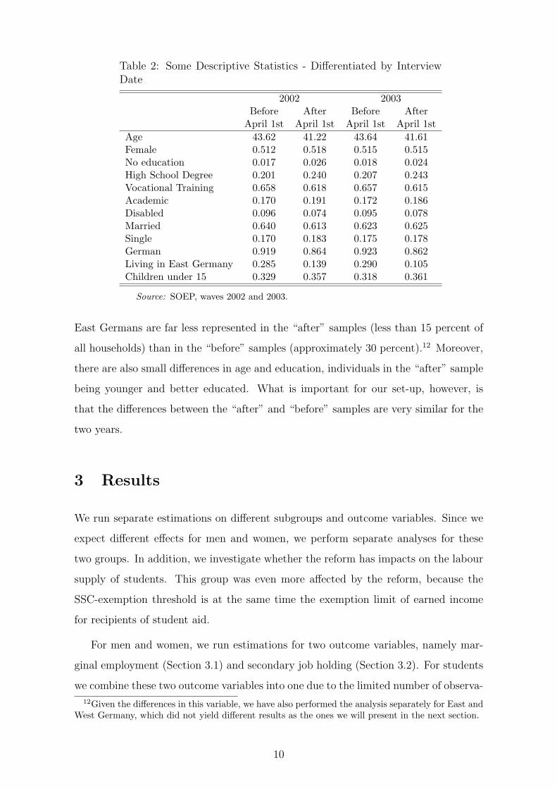
Table 2: Some Descriptive Statistics - Differentiated by InterviewDate
2002 2003Before After Before After
April 1st April 1st April 1st April 1stAge 43.62 41.22 43.64 41.61Female 0.512 0.518 0.515 0.515No education 0.017 0.026 0.018 0.024High School Degree 0.201 0.240 0.207 0.243Vocational Training 0.658 0.618 0.657 0.615Academic 0.170 0.191 0.172 0.186Disabled 0.096 0.074 0.095 0.078Married 0.640 0.613 0.623 0.625Single 0.170 0.183 0.175 0.178German 0.919 0.864 0.923 0.862Living in East Germany 0.285 0.139 0.290 0.105Children under 15 0.329 0.357 0.318 0.361
Source: SOEP, waves 2002 and 2003.
East Germans are far less represented in the “after” samples (less than 15 percent of
all households) than in the “before” samples (approximately 30 percent).12 Moreover,
there are also small differences in age and education, individuals in the “after” sample
being younger and better educated. What is important for our set-up, however, is
that the differences between the “after” and “before” samples are very similar for the
two years.
3 Results
We run separate estimations on different subgroups and outcome variables. Since we
expect different effects for men and women, we perform separate analyses for these
two groups. In addition, we investigate whether the reform has impacts on the labour
supply of students. This group was even more affected by the reform, because the
SSC-exemption threshold is at the same time the exemption limit of earned income
for recipients of student aid.
For men and women, we run estimations for two outcome variables, namely mar-
ginal employment (Section 3.1) and secondary job holding (Section 3.2). For students
we combine these two outcome variables into one due to the limited number of observa-
12Given the differences in this variable, we have also performed the analysis separately for East andWest Germany, which did not yield different results as the ones we will present in the next section.
10

tions (3.3). For all subgroups and outcome variables, we run three probit estimations,
respectively. The first estimation is only for the year 2003, and includes a dummy indi-
cating “interviewed after April 1st” as a single explanatory variable. This corresponds
to the “raw” effect of the reform, without controlling for potential seasonal effects or
possible differences in observable or unobservable characteristics between individuals
interviewed in and after the first quarter of 2003. In the second estimation, we control
for differences in observable characteristics by including a set of control variables such
as age, educational variables, regional variables, marital status, and number of chil-
dren. Finally, in the third estimation we pool data from 2002 and 2003, and include
two more variables, a dummy indicating the year 2003 and an interaction term between
this year dummy and the “interviewed after April 1st” dummy (see equation 4). Note
that this variable measures the effect that the “Mini-Job” reform had on the outcome
variable, controlling for seasonal effects, observable and unobservable characteristics
that differ between the groups interviewed in and after the first quarter of each year.
3.1 Effects on Marginal Employment
Table 3 shows a short summary of the estimation results for marginal employment,
where we have displayed marginal effects. Full estimation results, including the coef-
ficients and standard errors of the control variables, can be found in Table A.1 in the
Appendix. For men, the first model indicates that the “raw” effect of the reform is
positive, i.e. in the second and third quarter of 2003 we observe more men in mar-
ginal employment than in the first quarter of 2003. This is still true if we control for
differences in observable characteristics, as can be seen from column 2. The third col-
umn shows the estimation of the pooled sample of 2002 and 2003 including a dummy
variable indicating the year 2003, and an interaction term of this dummy with the
dummy indicating “interviewed after the reform”. We further interacted this variable
with the “single” dummy, because ex-ante studies have shown different reactions to
the reform by singles and individuals living with a partner. Doing so allows us to
calculate marginal effects for singles and couples separately.13 As our results show, as
13The marginal effect for individuals living in couples is computed as Φ(βafter + β2003 + βafter2003 +γ′X)−Φ(βafter + γ′X)−Φ(β2003 + γ′X)+Φ(γ′X) where Φ is the cdf of the normal distribution. Forsingles, the marginal effect corresponds to Φ(βafter + β2003 + βsingle + βafter2003 + βafter2003single +γ′X)− Φ(βafter + βsingle + γ′X)− Φ(β2003 + βsingle + γ′X) + Φ(βsingle + γ′X). The correspondingstandard errors are calculated using the Delta method.
11

far as the probability of being marginally employed is concerned, neither single men
nor men living in couples react to the reform.
Table 3: Estimation Results - Marginal Employment
Variable Men WomenModel 1 Model 2 Model 3 Model 1 Model 2 Model 3
Marg.Eff. Marg.Eff. Marg.Eff. Marg.Eff. Marg.Eff. Marg.Eff.after 0.0108* 0.0132** 0.0036 0.0246*** 0.0062 0.0171**
(0.0059) (0.0055) (0.0045) (0.0093) (0.0087) (0.0080)d2003 0.0045* 0.0195***
(0.0024) (0.0041)after×2003 (Couples) 0.0090 -0.0092
(0.0067) (0.0108)after×2003 (Singles) 0.0145 -0.0158
(0.0135) (0.0247)Controlled for Covariates no yes yes no yes yesLog-Likelihood -1666.813 -1529.5 -2919.3 -3829.5 -3664.7 -7183.4Observations 8,907 8,907 18,154 9,444 9,444 19,215
Note: ***/**/* indicates significance at the 1%/5%/10% level. Standard errors (in parentheses) correctfor correlation across repeated observations of individuals.Covariates include: age, age2, no education, high school degree, vocational training, academic, disabled,married, single, german, number of children in different age classes, and a dummy for living in EastGermany. See also Table A.1.Source: Estimations based on SOEP, waves 2002 and 2003.
Similar to what we observe for men, we find a positive and significant “raw” effect
of the reform for women (see column 4). This effect disappears, however, if we control
for socio-demographics (column 5) and for differences in seasonal employment effects
and unobservable characteristics between the “before” and “after” samples (column
6). Note that in the full model presented in column 6, the coefficients of the variables
after and d2003 are positive and significant, indicating that for women the probability
of being marginally employed is higher in the second and third quarter of each year,
and that this probability is also higher in 2003. However, there is no causal effect of
the reform, which would be caught by the effect of the variables after × 2003 and
after × 2003× single (see Table A.1 in the Appendix).
Thus, our first conclusion is that in the short-run (defined as about two months
after the reform), there has not been a significant change in marginal employment that
could be causally related to the legislation introduced on April 1st, 2003. However,
at least for women, marginal employment seems to be higher in the summer months
than in winter and higher in 2003 than in 2002.
12

3.2 Effects on Secondary Job Holding
Let us now turn to the analysis of the probability of holding a secondary job. As
already explained above, for these estimations we focus on the sample of full-time or
part-time employed individuals only. As Table 4 (column 1) shows, there seems to
be no significant “raw” effect of the reform for men, as the share of men holding a
secondary job does not differ between the first and the subsequent quarters of 2003.14
This is also true if we control for differences in observed characteristics (column 2) and
for differences in seasonal employment effects and unobserved characteristics (column
3).
Table 4: Estimation Results - Secondary Employment
Variable Men WomenModel 1 Model 2 Model 3 Model 1 Model 2 Model 3
Marg.Eff. Marg.Eff. Marg.Eff. Marg.Eff. Marg.Eff. Marg.Eff.after 0.0058 0.0051 0.0012 0.0030 0.0004 0.0001
(0.0066) (0.0062) (0.0054) (0.0068) (0.0062) (0.0057)d2003 0.0017 -0.0009
(0.0030) (0.0033)after×2003 (Couples) -0.0015 0.0017
(0.0072) (0.0087)after×2003 (Singles) 0.0311 -0.0023
(0.0198) (0.0207)Controlled for Covariates no yes yes no yes yesLog-Likelihood -929.1 -891.6 -1794.2 -665.8 -644.4 -1324.8Observations 5,564 5,564 11,466 4,447 4,447 9,047
Note: ***/**/* indicates significance at the 1%/5%/10% level. Standard errors (in parentheses) correctfor correlation across repeated observations of individuals.Covariates include: age, age2, no education, high school degree, vocational training, academic, disabled,married, single, german, number of children in different age classes, a dummy for living in East Germany,industry class, full-time employment dummy, and overtime. See also Table A.2.Source: Estimations based on SOEP, waves 2002 and 2003.
However, as the results of this estimation show (see Table A.2 in the Appendix), we
do find a positive effect for single men that is significant at the 10 percent level. The
marginal effect corresponding to this coefficient amounts to 0.031. This implies that
for single men, the probability of having a secondary job increases by 3.1 percentage
points. Since the probability of holding a secondary job before the reform for single
men is 3.7 percent, this effect almost implies a doubling of secondary employment in
this group. However, the standard error of the marginal effect amounts to 0.0198.15
14Full estimation results can be found in Table A.2 in the Appendix.15Statistical (non)significance of the estimated coefficient of the interaction term does not neces-
13

The marginal effect is thus not significant at the 10 percent level, the empirical signifi-
cance level amounting to 11.5%. Given the economic significance of the effect and the
relatively limited number of observations, we would not conclude from the standard
error that the reform did not affect this group, but rather that there is evidence for a
positive effect on secondary employment of single men. As columns 4 to 6 of Table 4
show, we do not find a corresponding effect for women.
3.3 Effects for Students
The estimation results for students can be found in Table 5.16
Table 5: Estimation Results - Marginal and/or SecondaryEmployment for Students
Variable StudentsModel 1 Model 2 Model 3
Marg.Eff. Marg.Eff. Marg.Eff.after 0.0639*** 0.0500** 0.0465**
(0.0220) (0.0220) (0.0193)d2003 0.0379***
(0.0112)after×2003 0.0042
(0.0267)Controlled for Covariates no yes yesLog-Likelihhod -1161.7 -1134.1 -2197.5Observations 2,295 2,295 4,703
Note: ***/**/* indicates significance at the 1%/5%/10% level.Standard errors (in parentheses) correct for correlation across re-peated observations of individuals.Covariates include: age, age2, no education, high school degree,vocational training, academic, disabled, married, single, german,number of children in different age classes, and a dummy for livingin East Germany. See also Table A.4.Source: Estimations based on SOEP, waves 2002 and 2003.
Similar to what we found for women with respect to marginal employment, for
students there is a positive and significant “raw” effect of the reform, in that students
in the second and third quarter of 2003 are more likely to be observed in marginal
employment or holding a secondary job than in the first quarter of 2003. This is
sarily imply (non)significance of the marginal effect of this variable in non-linear models (see Ai andNorton, 2003).
16Table A.3 in the Appendix contains the total number of observations for this group as well as thenumbers on being marginal employed and/or holding a secondary job. Due to the limited number ofobservations we pooled male and female observations and included a control variable for gender. Fullestimation results can be found in Table A.4 in the Appendix.
14

still true once we control for socio-demographic characteristics. The difference-in-
differences model, however, shows that there is no causal effect of the reform, even
though the probability of being marginally employed or holding a secondary job is
higher in 2003 and in the second and third quarter of each year.17
To sum up, we find that in the short run, there is evidence that the reform had a
causal effect for single men, whose probability of having a secondary job increases by
about three percent. According to our estimation results, the reform had no causal
effect on marginal employment in any of the subgroups.
4 Conclusions
The aim of this paper was to evaluate the causal effect of the German “Mini-Job”
reform from 2003 on the probabilities of being in marginal employment or of having a
secondary job. Based on our identification strategy, we were able to identify the short-
run effects of the reform. We could not find a significant effect on the probability of
being marginally employed for any subgroup. However, we found evidence that the
probability of having a secondary job increases for single men.
All ex-ante evaluation studies using behavioural microsimulation models predict
similar effects from the “Mini-Job” reform. They find a small yet significant effect
on the labour force participation of women living in couple households. As described
above, we do not find a significant effect on the participation in marginal employment
in the short run. However, since the effects that are calculated with ex-ante microsim-
ulation techniques correspond to long-term effects, our results need not necessarily be
a contradiction to this literature. The effect of the “Mini-Job” reform on students, as
well as on secondary job holding has not been analysed so far. However, as we show,
secondary job holding is the only outcome variable for which we find any short-run
effect, at least for the group of single men.
The numbers published by official sources portrayed the “Mini-Job” reform as quite
successful in generating new employment. The Federal Ministry of Health and Social
Affairs stated in July 2003 that three months after the reform, 930,000 new jobs had
been created. These numbers were corrected by the Federal Employment Agency in
17We also ran the same model including the variable after2003× single, which did not change theresults.
15

November 2003, who stated that one month after the reform, there was an increase
in marginal employment of as high as 79,000 individuals and an increase of secondary
jobs by 580,000. As stated above, we did not find any significant effects on marginal
employment. This could be due to various reasons. First, while we showed that for
women and students marginal employment is higher in the summer months and in
2003, our results show that there is no significant causal effect of the reform. Thus,
our conclusion is that the immediate increase in marginal employment of 79,000 jobs
cannot be causally related to the reform. As far as secondary jobs are concerned,
our results differ to a much larger extent from the numbers published by the Federal
Employment Agency. We only find evidence for a positive reaction to the reform among
single men, whose probability of having a secondary job increases. However, this can
not explain the total increase of 580,000 secondary jobs stated above. We believe that
a large fraction of these “new” jobs are actually redefinitions of previously fake self-
employment. This effect cannot be identified with the SOEP data. The same is true
for turning illegal jobs into legal employment (see also Schupp and Birkner, 2004).
Thus, we conclude that in the short-run, the reform had a very limited causal
impact on the labour supply in Germany. The high numbers that circulated in the press
in the first months after the reform were to a great extent referring to (i) additional
jobs that have been created not due to the reform but to seasonal employment effects
and the general trend of increasing marginal employment and (ii) to redefinitions of
already existing jobs or the turning of illegal jobs into legal employment.
16

References
Ai, C., and E. Norton (2003): “Interaction terms in logit and probit models,”Economics Letters, 80, 123–129.
Arntz, M., M. Feil, and A. Spermann (2003): “Die Arbeitsangebotseffekteder neuen Mini- und Midijobs - eine Ex-Ante Evaluation,” Mitteilungen aus derArbeitsmarkt- und Berufsforschung, 3/2003.
Bargain, O., M. Caliendo, P. Haan, and K. Orsini (2006): “‘Making WorkPay’ in a Rationed Labour Market,” Discussion Paper No. 2033, IZA Bonn.
Blundell, R. (2000): “Work Initiatives and ’in-work’ Benefit Reforms: A Review,”Oxford Review of Economic Policy, 16, 27–44.
Blundell, R., A. Duncan, J. McCrae, and C. Meghir (2000): “The LabourMarket impact of the Working Families Tax Credit,” Fiscal Studies, 21(1), 75–104.
Bundesagentur fur Arbeit (2003): “Erste statistische Ergebnisse ueber Minijobsnach der gesetzlichen Neuregelung zum 1. April 2003,” Press release november 2003,Bundesanstalt fuer Arbeit.
Haan, P., and V. Steiner (2005): “Distributional Effects of the German TaxReform 2000 - A Behavioral Microsimulation Analysis,” Journal of Applied SocialScience Studies, 125, 39–49.
Haisken De-New, J., and J. Frick (2003): Desktop Compendium to The GermanSocio-Economic Panel Study (SOEP). DIW, Berlin.
Heckman, J., R. LaLonde, and J. Smith (1999): “The Economics and Economet-rics of Active Labor Market Programs,” in Handbook of Labor Economics Vol.III,ed. by O. Ashenfelter, and D. Card, pp. 1865–2097. Elsevier, Amsterdam.
Moffitt, R. (2003): “Welfare Program and Labor Supply,” Working Paper 9168,NBER.
Orsini, K. (2006): “Tax-Benefit Reform and the Labor Market: Evidence from Bel-gium and other EU countries,” Mimeo.
Roy, A. (1951): “Some Thoughts on the Distribution of Earnings,” Oxford EconomicPapers, 3(2), 135–145.
Rubin, D. (1974): “Estimating Causal Effects to Treatments in Randomised andNonrandomised Studies,” Journal of Educational Psychology, 66, 688–701.
Scholz, J. K. (1996): “In-Work Benefits in the United States: The Earned IncomeTax Credit,” The Economic Journal, 106, 156–169.
Schupp, J., and E. Birkner (2004): “Kleine Beschaftigungverhaltnisse: Kein Job-wunder,” Wochenbericht No. 34/2004, DIW, Berlin.
Stancanelli, E. (2005): “Evaluating the Impact of the French Tax Credit Pro-gramme, ”La Prime Pour L’Emploi”: A Difference in Difference Model,” WorkingPaper, OFCE.
Steiner, V., and K. Wrohlich (2005): “Work Incentives and Labour SupplyEffects of the Mini-Jobs Reform in Germany,” Empirica, 32, 91–116.
17

Appendix - Tables
Table A.1: Estimation Results - Marginal Employment - Full Model 1
Variable Men WomenModel 1 Model 2 Model 3 Model 1 Model 2 Model 3
Coef. Coef. Coef. Coef. Coef. Coef.after 0.106* 0.148** 0.05 0.107*** 0.029 0.083**
(0.055) (0.059) (0.058) (0.039) (0.04) (0.038)d2003 0.062* 0.097***
(0.032) (0.020)after×2003 0.095 -0.05
(0.081) (0.051)after×2003×single 0.029 -0.021
(0.132) (0.099)age -0.121*** -0.119*** 0.025*** 0.018**
(0.011) (0.009) (0.009) (0.007)age squared 0.001*** 0.001*** -0.000*** -0.000***
(0.000) (0.000) (0.000) (0.000)no education -0.293 -0.225 -0.202 -0.215*
(0.228) (0.163) (0.131) (0.120)high-school degree 0.392*** 0.349*** 0.067 0.021
(0.065) (0.057) (0.048) (0.043)vocational training -0.026 -0.057 -0.156*** -0.163***
(0.062) (0.049) (0.039) (0.034)academic -0.221*** -0.258*** -0.358*** -0.364***
(0.080) (0.075) (0.058) (0.054)disabled -0.029 0.041 -0.307*** -0.234***
(0.084) (0.073) (0.075) (0.06)single -0.006 -0.022 -0.013 0.01
(0.073) (0.062) (0.055) (0.047)married -0.222*** -0.206*** 0.195*** 0.220***
(0.079) (0.063) (0.053) (0.043)german -0.033 0.014 0.184*** 0.219***
(0.093) (0.077) (0.062) (0.055)children under 15 -0.033 -0.056
(0.065) (0.052)children under 1 -0.234** -0.199***
(0.099) (0.074)children under 7 0.069 0.058
(0.048) (0.039)children between 8-15 0.185*** 0.202***
(0.040) (0.033)east german 0.039 0.032 -0.309*** -0.344***
(0.057) (0.049) (0.043) (0.037)constant -1.705*** 0.598*** 0.486*** -1.101*** -1.493*** -1.495***
(0.026) (0.218) (0.182) (0.018) (0.168) (0.139)Log-Likelihood -1666.8 -1529.5 -2919.3 -3829.5 -3664.7 -7183.4Observations 8,907 8,907 18,154 9,444 9,444 19,215
Note: ***/**/* indicates significance at the 1%/5%/10% level. Standard errors (in parenthe-ses) are corrected for correlation across repeated observations of individuals.All variables except age and age squared are dummy variables, taking the value 1 if the con-dition is fulfilled.Source: Estimations based on SOEP, waves 2002 and 2003.
18

Table A.2: Estimation Results - Secondary Employment - Full Model 1
Variable Men WomenModel 1 Model 2 Model 3 Model 1 Model 2 Model 3
Coef. Coef. Coef. Coef. Coef. Coef.after 0.066 0.065 0.015 0.038 0.006 0.001
(0.072) (0.076) (0.071) (0.086) (0.090) (0.081)d2003 0.023 -0.012
(0.039) (0.047)after×2003 -0.02 0.024
(0.096) (0.122)after×2003×single 0.320* -0.041
(0.172) (0.179)age 0.02 0.043** 0.001 0.003
(0.025) (0.021) (0.027) (0.020)age squared -0.000 -0.001** -0.000 -0.000
(0.000) (0.000) (0.000) (0.000)no education -0.058 -0.404 0.506* 0.38
(0.415) (0.387) (0.294) (0.251)vocational training 0.234*** 0.113 -0.013 -0.059
(0.087) (0.07) (0.092) (0.074)academic 0.108 0.091 0.185* 0.195**
(0.084) (0.07) (0.099) (0.081)disabled 0.067 0.072 -0.154 0.046
(0.144) (0.116) (0.203) (0.140)married 0.131 0.077 -0.124 -0.038
(0.098) (0.082) (0.107) (0.085)single 0.117 -0.028 0.163 0.242***
(0.103) (0.096) (0.107) (0.083)german 0.164 0.166 -0.096 0.027
(0.133) (0.112) (0.143) (0.120)children under 15 -0.08 -0.059
(0.079) (0.065)children under 1 -0.072 -0.100
(0.123) (0.097)children between 8-15 -0.137 -0.108
(0.098) (0.075)east german -0.121 -0.142** -0.156 -0.122
(0.082) (0.070) (0.097) (0.076)civil servant 0.119 0.084 -0.320* -0.320**
(0.116) (0.099) (0.180) (0.134)self-employed -0.377*** -0.293*** -0.18 -0.255
(0.138) (0.110) (0.184) (0.163)industry class. 2 -0.107 -0.057 0.046 -0.066
(0.108) (0.093) (0.176) (0.166)industry class. 3 0.031 0.124 -0.101 -0.148
(0.122) (0.099) (0.142) (0.112)industry class. 4 -0.181 -0.165 -0.326 -0.264
(0.160) (0.126) (0.296) (0.248)industry class. 5 0.184** 0.231*** 0.169 0.134
(0.093) (0.079) (0.107) (0.090)industry class. 6 0.109 0.196** -0.112 -0.020
(0.119) (0.099) (0.155) (0.116)industry class. 7 0.16 0.139 0.275* 0.257**
(0.139) (0.115) (0.151) (0.124)Continued on next page.
19

Table A.2 continued.Variable Men Women
Model 1 Model 2 Model 3 Model 1 Model 2 Model 3Coef. Coef. Coef. Coef. Coef. Coef.
overtime (< 3h) -0.056 0.027 0.105 0.123*(0.087) (0.067) (0.087) (0.064)
overtime (≥ 3h) 0.147** 0.163*** -0.024 0.007(0.075) (0.059) (0.109) (0.077)
full-time employed -0.507*** -0.560*** -0.069 -0.148**(0.140) (0.109) (0.085) (0.068)
constant -1.769*** -1.930*** -2.348*** -1.828*** -1.693*** -1.797***(0.035 (0.502) (0.402) (0.041 (0.532) (0.397)
Log-Likelihood -929.1 -891.6 -1794.2 -665.8 -644.4 -1324.8Observations 5564 5564 11466 4447 4447 9047
Note: ***/**/* indicates significance at the 1%/5%/10% level. Standard errors (in paren-theses) are corrected for correlation across repeated observations of individuals.All variables except age and age squared are dummy variables, taking the value 1 if thecondition is fulfilled.Source: Estimations based on SOEP, waves 2002 and 2003.
Table A.3: Number of Observations, Marginaland/or Secondary Employment for Students inthe Subsamples1
Marg. or Secon.Employment
Subsample Obs. abs. in %before 1778 274 0.05742002after
April 1st630 132 0.0873
before 1819 350 0.08082003after
April 1st476 122 0.1324
Note: High income sample of the SOEP is not in-cluded, since this entire group was interviewed afterApril in the 2003 wave. Numbers refer to the popula-tion in “Ausbildung”.Source: SOEP, waves 2002 and 2003.
20

Table A.4: Estimation Results - Marginal Employment - Full Model 1
Variable Students PensionerModel 1 Model 2 Model 3 Model 1 Model 2 Model 3
Coef. Coef. Coef. Coef. Coef. Coef.after 0.214*** 0.160** 0.159** 0.206** 0.142 -0.041
(0.071) (0.073) (0.068) (0.093) (0.096) (0.098d2003 0.145*** 0.034
(0.043) (0.042)after×2003 -0.005 0.179
(0.093) (0.123)age 0.060*** 0.048*** 0.001 0.023
(0.021) (0.018) (0.047) (0.045)female 0.204*** 0.229*** -0.151* -0.149**
(0.061) (0.049) (0.078) (0.067)age squared -0.001** -0.001** -0.000 -0.000
(0.000) (0.000) (0.000) (0.000)no education -0.168 -0.204
(0.281) (0.263)high-school degree 0.007 0.000
(0.137) (0.119)vocational training -0.239** -0.247*** 0.168* 0.148*
(0.096) (0.077) (0.092) (0.076)academic 0.222* 0.131
(0.122) (0.107)disabled -0.514 -0.331 -0.232*** -0.217***
(0.314) (0.207) (0.086) (0.074)single 0.033 0.083 -0.159 -0.011
(0.075) (0.060) (0.153) (0.138)married -0.388*** -0.351*** -0.148 -0.028
(0.136) (0.105) (0.141) (0.131)german 0.283** 0.178* 0.145 0.257*
(0.126) (0.102) (0.179) (0.155)children under 15 -0.134* -0.06 -0.275 -0.144
(0.071) (0.055) (0.270) (0.171)east german -0.224*** -0.246*** -0.279*** -0.314***
(0.071) (0.058) (0.088) (0.075)constant -0.869*** -2.025*** -1.889*** -1.523*** -0.818 -1.519
(0.034 (0.342) (0.285) (0.040) (1.283) (1.264)Log-Likelihhod -1161.7 -1134.1 -2197.5 -701.6 -683.9 -1319.9Observations 2,295 2,295 4,703 2,821 2,821 5,671
Note: ***/**/* indicates significance at the 1%/5%/10% level. Standard errors (in paren-theses) are corrected for correlation across repeated observations of individuals.All variables except age and age squared are dummy variables, taking the value 1 if thecondition is fulfilled.Source: Estimations based on SOEP, waves 2002 and 2003.
21