Embed Size (px)
Citation preview
Walden UniversityScholarWorks
Walden Dissertations and Doctoral Studies Walden Dissertations and Doctoral StudiesCollection
1-1-2009
Evaluating earnings management with derivativesand the use of accounting accruals: A quasiexperimental approachMargot S. GeagonWalden University
Follow this and additional works at: https://scholarworks.waldenu.edu/dissertations
Part of the Accounting Commons, Finance and Financial Management Commons, and theStatistics and Probability Commons
This Dissertation is brought to you for free and open access by the Walden Dissertations and Doctoral Studies Collection at ScholarWorks. It has beenaccepted for inclusion in Walden Dissertations and Doctoral Studies by an authorized administrator of ScholarWorks. For more information, pleasecontact [email protected].

Walden University
COLLEGE OF MANAGEMENT AND TECHNOLOGY
This is to certify that the doctoral dissertation by
Margot S. Geagon
has been found to be complete and satisfactory in all respects, and that any and all revisions required by the review committee have been made.
Review Committee Dr. Thomas Spencer, Committee Chairperson,
Applied Management and Decision Sciences Faculty
Dr. Robert O’Reilly, Committee Member, Applied Management and Decision Sciences Faculty
Dr. Jeffrey Prinster Committee Member, Applied Management and Decision Sciences Faculty
Chief Academic Officer
Denise DeZolt, Ph.D.
Walden University 2009

ABSTRACT
Evaluating Earnings Management with Derivatives and the use of Accounting Accruals: A Quasi Experimental Approach
by
Margot S. Geagon
M.B.A., Marylhurst University, 2003 M.P.A., Portland State University, 2002
B.A., Western New Mexico University, 1999
Dissertation Submitted in Partial Fulfillment of the Requirements for the Degree of
Doctor of Philosophy Applied Management Decision Sciences
Walden University August 2009
ABSTRACT
Most companies listed on the S&P 500 index have reported smoothed earnings since the 1990s
inspiring questions from regulators about the accuracy of financial statements. In 1998, the
Financial Accounting Standards Board issued SFAS No. 133 (Accounting for Derivative
Instruments and Hedging Activities) to establish accounting and reporting standards for
derivative instruments. In 2002, the Sarbanes-Oxley Act (SOX) was issued to eradicate earnings
management activities and improve transparency in financial reporting. Although many studies
have been conducted to evaluate changes in reporting requirements, much less is known about the
effectiveness of these regulations on earning smoothing with discretionary accruals (DA) and
derivative hedge reporting (DHR). Accordingly, this study was an investigation of the
effectiveness of SOX and SFAS No. 133 on DA, and DHR. The research questions were used to
examine DA, and to evaluate the transparency of DHR for the years 1997 through 2007. This
study is a quasi-experimental research design where 30 companies from the high technology
industry segment were randomly drawn to form 330 observations. The modified Jones model was
used to separate DA and repeated measures analyses of variance were used to assess differences
in levels before and after the issuance of SOX. A Quality Disclosure Index (QDI) was used to
assess the transparency of DHR and repeated measures of variance were used to evaluate the QDI
scores before and after the issuance of SFAS No. 133. The findings suggest DA activities are
decreasing but represent over 50% of total net accruals for all years and the QDI for DHR is
decreasing. Improved financial regulation is needed. The study contributes to positive social
change by providing regulators and investors with new information about accruals for income
conservative firms by segmenting DA and investigating the level of transparency in DHR that
could be used to formulate appropriate financial regulation and improve the quality of our
financial reporting system.

Evaluating Earnings Management with Derivatives and the use of Accounting Accruals: A Quasi Experimental Approach
by
Margot S. Geagon
M.B.A., Marylhurst University, 2003 M.P.A., Portland State University, 2002
B.A., Western New Mexico University, 1999
Dissertation Submitted in Partial Fulfillment of the Requirements for the Degree of
Doctor of Philosophy Applied Management Decision Sciences
Walden University August 2009

UMI Number: 3366971
INFORMATION TO USERS
The quality of this reproduction is dependent upon the quality of the copy
submitted. Broken or indistinct print, colored or poor quality illustrations and
photographs, print bleed-through, substandard margins, and improper
alignment can adversely affect reproduction.
In the unlikely event that the author did not send a complete manuscript
and there are missing pages, these will be noted. Also, if unauthorized
copyright material had to be removed, a note will indicate the deletion.
______________________________________________________________
UMI Microform 3366971 Copyright 2009 by ProQuest LLC
All rights reserved. This microform edition is protected against unauthorized copying under Title 17, United States Code.
_______________________________________________________________
ProQuest LLC 789 East Eisenhower Parkway
P.O. Box 1346 Ann Arbor, MI 48106-1346

DEDICATION
This dissertation is lovingly dedicated to my husband, Patrick. You are my soul mate and
have always stood by me with love, support, and understanding. Your encouragement and
guidance has helped me complete this enriching and wonderful scholastic journey.

ii
ACKNOWLEDGMENTS
I wish to thank my dissertation committee chair Dr. Thomas Spencer, and committee
members, Dr. Robert O'Reilly and Dr. Jeff Prinster. Dr. Thomas Spencer has been an integral
factor in my success and I greatly appreciate his continued support. To you, my dissertation
committee, I extend my heartfelt gratitude for all your hard work. I would also like to thank Dr.
Lawrence Ness and Ms. Annie Pezalla for their contributions to this study. Most of all, I want to
thank my husband, Patrick, for helping me keep my feet on the ground while reaching for the
stars.

iii
TABLE OF CONTENTS
LIST OF TABLES ........................................................................................................................ V
LIST OF FIGURES ..................................................................................................................... VI
CHAPTER 1: INTRODUCTION TO THE STUDY .................................................................. 1
PROBLEM STATEMENT ................................................................................................................. 6 NATURE OF THE STUDY ............................................................................................................... 8 RESEARCH QUESTIONS .............................................................................................................. 11 PURPOSE OF STUDY ................................................................................................................... 16 THEORETICAL FRAMEWORK ...................................................................................................... 17
Discretionary Accrual Modeling ........................................................................................... 19DEFINITION OF TERMS ............................................................................................................... 20 LIMITATIONS AND DELIMITATIONS ........................................................................................... 21 SIGNIFICANCE OF THE STUDY .................................................................................................... 21
CHAPTER 2: LITERATURE REVIEW ................................................................................... 23
REVIEW OF RELATED RESEARCH .............................................................................................. 24 DISCRETIONARY ACCRUALS ACTIVITY UNDER SOX ................................................................ 25
Earnings Management through GAAP Discretions .............................................................. 26Discretionary Accruals ......................................................................................................... 27
A NEW APPROACH TO EVALUATING ACCRUALS ...................................................................... 28 Evaluating Abnormal Accruals ............................................................................................. 28Discretionary Accrual Modeling ........................................................................................... 30Calculation of Accruals ......................................................................................................... 31Accrual Modeling and Statistical Distribution Methodology ............................................... 32Direct Cash Flow Earnings Management Methodology ....................................................... 36
DERIVATIVE HEDGING AND SYSTEMATIC RISK ........................................................................ 37 Derivative Hedging Incentives .............................................................................................. 37Derivative Hedging ............................................................................................................... 39Derivatives and SFAS No.133 Accounting Discretion .......................................................... 41Earnings Management with Derivative Hedging .................................................................. 41Disclosure Quality of Derivative Reporting .......................................................................... 44
CHAPTER 3: RESEARCH METHOD ..................................................................................... 46
RESEARCH DESIGN AND APPROACH .......................................................................................... 47 Cross-Sectional Analysis ....................................................................................................... 49
SETTING AND SAMPLE ............................................................................................................... 50 TREATMENT ............................................................................................................................... 52
Research Question 1 ............................................................................................................. 53Research Question 2 ............................................................................................................. 54Research Question 3 ............................................................................................................. 55Research Question 4 ............................................................................................................. 56Research Question 5 ............................................................................................................. 56
INSTRUMENTATION AND MATERIALS ........................................................................................ 60 Measures Taken for the Protection of Participants’ Rights .................................................. 62
SUMMARY .................................................................................................................................. 62
iv
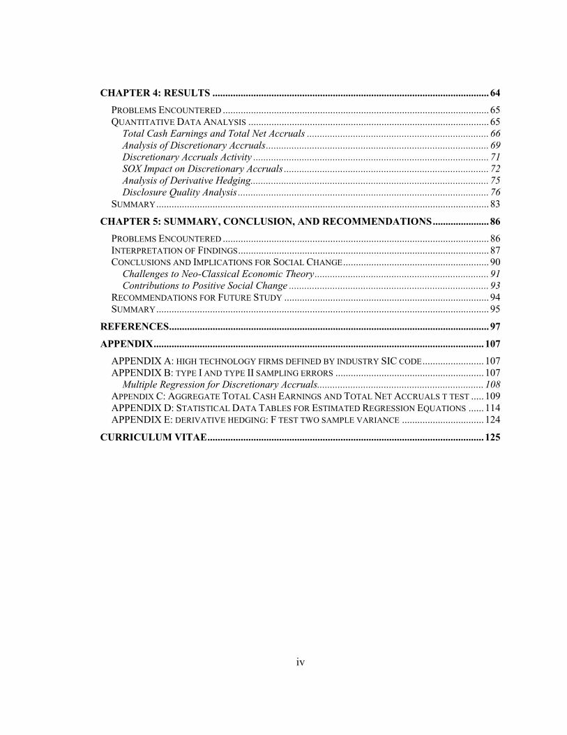
CHAPTER 4: RESULTS ............................................................................................................ 64
PROBLEMS ENCOUNTERED ........................................................................................................ 65 QUANTITATIVE DATA ANALYSIS .............................................................................................. 65
Total Cash Earnings and Total Net Accruals ....................................................................... 66Analysis of Discretionary Accruals ....................................................................................... 69Discretionary Accruals Activity ............................................................................................ 71SOX Impact on Discretionary Accruals ................................................................................ 72Analysis of Derivative Hedging ............................................................................................. 75Disclosure Quality Analysis .................................................................................................. 76
SUMMARY .................................................................................................................................. 83
CHAPTER 5: SUMMARY, CONCLUSION, AND RECOMMENDATIONS ...................... 86
PROBLEMS ENCOUNTERED ........................................................................................................ 86 INTERPRETATION OF FINDINGS .................................................................................................. 87 CONCLUSIONS AND IMPLICATIONS FOR SOCIAL CHANGE ......................................................... 90
Challenges to Neo-Classical Economic Theory .................................................................... 91Contributions to Positive Social Change .............................................................................. 93
RECOMMENDATIONS FOR FUTURE STUDY ................................................................................ 94 SUMMARY .................................................................................................................................. 95
REFERENCES ............................................................................................................................. 97
APPENDIX ................................................................................................................................. 107
APPENDIX A: HIGH TECHNOLOGY FIRMS DEFINED BY INDUSTRY SIC CODE ........................ 107 APPENDIX B: TYPE I AND TYPE II SAMPLING ERRORS .......................................................... 107
Multiple Regression for Discretionary Accruals................................................................. 108APPENDIX C: AGGREGATE TOTAL CASH EARNINGS AND TOTAL NET ACCRUALS T TEST ..... 109 APPENDIX D: STATISTICAL DATA TABLES FOR ESTIMATED REGRESSION EQUATIONS ...... 114 APPENDIX E: DERIVATIVE HEDGING: F TEST TWO SAMPLE VARIANCE ................................ 124
CURRICULUM VITAE ............................................................................................................ 125
v
LIST OF TABLES
TABLE 1 RESEARCH QUESTION 1: RESEARCH APPROACH ............................................................. 12 TABLE 2 RESEARCH QUESTION 2: RESEARCH APPROACH ............................................................. 13 TABLE 3 RESEARCH QUESTION 3: RESEARCH APPROACH ............................................................. 14 TABLE 4 RESEARCH QUESTION 4: RESEARCH APPROACH ............................................................. 15 TABLE 5 RESEARCH QUESTION 5: RESEARCH APPROACH ............................................................. 16 TABLE 7 AGGREGATE T TESTS RESULTS FOR TOTAL CASH EARNINGS AND TOTAL NET
ACCRUALS ............................................................................................................................. 68 TABLE 8 ESTIMATED REGRESSION COEFFICIENTS ......................................................................... 69 TABLE 9 ESTIMATED REGRESSION EQUATIONS ............................................................................. 70 TABLE 10 DISCRETIONARY ACCRUALS ACTIVITY: YEARS 1997 – 2007 ....................................... 72 TABLE 11 AVERAGE QDI SCORES: YEARS 1997 - 2007 ................................................................ 77 TABLE 6 HIGH TECHNOLOGY INDUSTRY DEFINED BY SIC CODE ................................................ 107 1997 T-TEST: TWO-SAMPLE ASSUMING UNEQUAL VARIANCES .................................................. 109 1998 T-TEST: TWO-SAMPLE ASSUMING UNEQUAL VARIANCES .................................................. 109 1999 T-TEST: TWO-SAMPLE ASSUMING UNEQUAL VARIANCES .................................................. 110 2000 T-TEST: TWO-SAMPLE ASSUMING UNEQUAL VARIANCES .................................................. 110 2001 T-TEST: TWO-SAMPLE ASSUMING UNEQUAL VARIANCES .................................................. 110 2002 T-TEST: TWO-SAMPLE ASSUMING UNEQUAL VARIANCES .................................................. 111 2003 T-TEST: TWO-SAMPLE ASSUMING UNEQUAL VARIANCES .................................................. 111 2004 T-TEST: TWO-SAMPLE ASSUMING UNEQUAL VARIANCES .................................................. 112 2005 T-TEST: TWO-SAMPLE ASSUMING UNEQUAL VARIANCES .................................................. 112 2006 T-TEST: TWO-SAMPLE ASSUMING UNEQUAL VARIANCES .................................................. 113 2007 T-TEST: TWO-SAMPLE ASSUMING UNEQUAL VARIANCES .................................................. 113 T-TEST: TWO-SAMPLE ASSUMING UNEQUAL VARIANCES: YEARS 1997 - 2007 .......................... 113 1997 STATISTICAL SUMMARY ..................................................................................................... 114 1998 STATISTICAL SUMMARY ..................................................................................................... 115 1999 STATISTICAL SUMMARY ..................................................................................................... 116 2000 STATISTICAL SUMMARY ..................................................................................................... 117 2001 STATISTICAL SUMMARY ..................................................................................................... 117 2002 STATISTICAL SUMMARY ..................................................................................................... 118 2004 STATISTICAL SUMMARY ..................................................................................................... 120 2005 STATISTICAL SUMMARY ..................................................................................................... 121 2006 STATISTICAL SUMMARY ..................................................................................................... 122 2007 STATISTICAL SUMMARY ..................................................................................................... 123
vi
LIST OF FIGURES
Figure 1. t tests for total net accruals and total cash earnings ......................................... 108
Figure 2. Multiple regressions for discretionary accruals ............................................... 109
Figure 3. Policy information questions ............................................................................. 57
Figure 4. Hedges of anticipated transactions .................................................................... 57
Figure 5. Risk information ................................................................................................ 58
Figure 6. Net fair value information ................................................................................. 58
Figure 7. Disclosure quality .............................................................................................. 59
Figure 8. Average total cash earnings & average total net accruals: 1997 – 2007 ........... 67
Figure 9. Total accrual activity years: 1997 – 2007 .......................................................... 71
Figure 10. Proportion of discretionary accruals in 2000 and 2005 ................................... 73
Figure 11. Discretionary accrual usage: Year 2000 .......................................................... 74
Figure 12. Discretionary accrual usage: Year 2005 .......................................................... 74
Figure 13. The rate of change in derivative hedging ........................................................ 76
Figure 14. Average policy information score for years 1997 – 2007 ............................... 78
Figure 15. Average risk information score for years 1997 – 2007 ................................... 78
Figure 16. Average anticipated hedging score for years 1997 – 2007 .............................. 79
Figure 17. Average net fair value scores for years 1997 – 2007....................................... 80
Figure 18. Average QDI scores for years 1997 – 2007 .................................................... 80
Figure 19. QDI scores for year 1998 ................................................................................ 81
Figure 20. QDI scores for year 2002 ................................................................................ 82
Figure 21. QDI population proportion for years 1998 – 2002 .......................................... 83
CHAPTER 1:
INTRODUCTION TO THE STUDY
Within the finance discipline, the analysis of earnings management through the use of
discretionary accruals is in the early stages of development. Axioms and standards for a model to
evaluate the degree of discretionary activities have not yet been established. Several divergent
attempts have been made to explore management choices through the use of accounting accruals
and the results of these peer-reviewed studies have been mixed. To date, the high technology
industry segment within the U.S. has not been isolated from other industry sectors in the
evaluation of discretionary accruals. Firms in the technology industry segment differ from other
industry segments in that they engage in income conservative practices more frequently and are
exposed to higher levels of risk to shareholder litigation (Lobo, Zhou, 2006). In addition, high
tech industry companies are also affected to a greater degree by conservative accounting
standards on research and development costs (Uday, Wasley, & Waymire, 2004). This study fills
the knowledge gap of earnings management evaluation through the use of discretionary accruals
within the income conservative high technology industry segment.
Watts (2003) defined income conservatism as a higher verification standard applied to
favorable information resulting in lower cumulative earnings and net asset. The presence of
income conservatism is illustrated in significantly higher proportions of losses and lower average
profitability levels for technology firms relative to non-technology firms (Kwon, Yin, & Han,
2006). These differences mainly surface from differences in operating cash flow levels
attributable to research and development (R&D) expenses. The financial reporting of technology
firms also confirms the evidence of an increase in negative non-operating accruals (Uday, et. al.,
2004).

2
Earnings smoothing as defined by the act of minimizing earnings volatility is achieved
through the accounting treatment of transactions and or through the use of derivative contracts
forged to create a hedged financial position in situations where a significant amount of risk exists
(Bartov, Givoly, & Hayn, 2002). Managers utilize derivatives and accounting accruals to
minimize cash flow volatility, often referred to as earnings smoothing. In 1998, the Financial
Accounting Standards Board (FASB) issued a mandate (SFAS No. 133 Accounting for
Derivative Instruments and Hedging Activities), restricting firms from simultaneously recording
all offsetting gains and losses on items being hedged. Many critics (e.g., Bowen, Rajopal, &
Venkatchalam, 2004; Carter, Lynch, & Zechman, 2006; Cohen, Dev, & Lys, 2004; Liu, 2004)
assert SFAS No. 133 stimulates earnings volatility. However, in 2004 Stammerjohan conducted a
study of Fortune 500 firms to determine if derivative use either minimized in the face of the new
FASB mandate or whether cash flow volatility increased after of this new regulation. From his
study results, Stammerjohan (2004) concluded that although earnings volatility did increase
shortly after the release of the SFAS No. 133, this increase may be systemic of other factors
outside of the scope of the issuance of SFAS No. 133.
Earnings smoothing is a strategy used to deliberately manipulate the company's earnings
so that the figures match pre-determined targets (Glaum, Lichtblau, & Lindemann, 2004). This
practice is carried out for income smoothing; thus, rather than having years of exceptionally good
or bad earnings, companies will attempt to keep the figures relatively stable by adding and
removing cash from reserve accounts (Beattie, Brown, Manson, 1994). Although managers use
divergent methods to smooth earnings and these models can be complex, in-depth and
convoluted, the fundamental objective of these strategies is to meet pre-specified targets (Tucker,
& Zarowin, 2006).

3
Generally Accepted Accounting Principles (GAAP) are a set of widely accepted rules,
standards, and procedures for reporting financial information as established by the Financial
Accounting Standards Board. Under GAAP, firms are authorized to exercise discretion in
financial reporting in order to communicate managers’ information about performance (Zeff,
2005). This implies that managers can choose whether and how they will disclose information in
their financial reports.
A major concern of regulators and investors is that the accounting standards for financial
derivatives are still in the early stage, which cannot address all aspects of the multifaceted
financial derivatives market (International Monetary Fund Country report No 05/216). SFAS No.
133 (Accounting for Financial Derivatives and Hedging Activities) requires all financial
derivatives be reported at their fair value. The changes in fair value are either recognized as
earnings or deferred to future periods to offset the changes in the value of items being hedged.
The SFAS No. 133 standards provide discretions for earnings management (Singh, 2004). The
determination of the fair value of most derivative instruments are subject to many assumptions
such as those related to credit and liquidity risk resulting from the exclusion of derivative trading
from the trading market (Kawaller, 2004). Most derivative instruments are simply contracts
between a derivative dealer and the user firm, such as interest rate swaps (Leander, 1997).
Because derivative contracts are not actively traded in the market,their value has no
market reference (Dubofsky, & Miller, 2003). With no market reference, the value of the
derivative becomes variable and is largely based on the assumptions used in the analysis of the
fair market value (Naor, 2006) such as assumptions in the determination of the fair value of
derivatives and credit risk. The deferred derivative gains or losses to be reclassified into current
earnings are also subject to firms’ discretion, because the gains or losses of the items hedged do
not need to be reported separately under SFAS No. 133 (Kawaller, 2004).
4
Empirical research on earnings management and the valuation of earnings is heavily
researched in accounting journals; however, the approach to evaluate earnings management
through the use of discretionary accruals is still in the development phase. In 1996 (and revised in
1998), Dechow, Jowell Sabino, and Richard Sloan developed a model of non-discretionary
accruals that builds on related models in Jones (1991), Dechow (1994) and Dechow, Kothari and
Watts (1996). In 2003, Da Silva Rosa, Sheung, and Walter conducted a study to evaluate whether
bidding firms that offer shares as consideration engage in earnings management prior to takeover
announcements (Da Silva Rosa, Sheung, & Walter, 2000). The findings of their study show no
evidence of managing earnings upward.
Accruals are defined as the difference between cash flow from operations and net income
(Anderson, Caldwell, & Needles, 1994). A fundamental property of accruals is that they reverse
over time. The self-reversing property of accruals reduces the effecctiveness of any planned or
unplanned earnings management strategies when viewed in the aggregate over a long period of
time (Anderson, et.al., 1994). The characteristics of the reversing properties of accounting
accruals suggests that managers who utilize accruals through manipulation cannot rely on
accruals alone to report strong earnings and when the build-up accrual items invariably start to
unwind over time, they suppress future earnings and stock prices (Skinner, & Sloan, 2002).
Manipulation of accruals comes in many forms, from estimating earnings based on a
rolling average of a previous period such as a quarter to booking several prior months of accruals
in one period to reflect the number of months outstanding (Collins, & Hribar, 2000). Either
approach introduces uncertainty and skews the financial history of earnings for a firm, even if
reversals of these entries follow (Das, & Shroff, 2002). As a result, over time, managers may be
forced to make up earnings shortfalls with real cash earnings (Beattie, et al., 1994). Much of the
research focused on earnings management has investigated earnings management decisions

5
during particular events such takeover announcements (Da Silva Rosa, et.al., 2000), a shift in tax
laws (Mills and Newberry, 2001), or debt covenants (Dechow, 1996). Some managers may use
these extraneous occurances as justification for an increase in accruals (Mills et. al., 2001).
Accruals are used daily and are part of the operational expense structures of any firm that utilizes
accrual based accounting (Anderson, et.al., 1994); due to the use of accounting accruals in firms
who do now function under a cash basis, it is imperative that the use of accruals during standard
or regular periods of operation is investigated.
Previous literature based on eanrings management is based on the assumption that
accounting accruals and derivatives are used as tools in financial smoothing and earnings
management (Barton, 2001; Barton, & Simko, 2002; Bruns, & Merchant, 1990; Carter, Lynch, &
Zechman, 2006). However, Nissim and Penman (2003) claim that after the issuance of the
Sarbanes-Oxley Act (SOX) in 2002 by the Financial and Accounting Standards Board (FASB),
accrual models are ineffective in detecting earnings management and Cohen, Dey, and Lys
(2005) asserted firms tend to refer to actual transactions rather than accruals in earnings
smoothing. These arguments introduce questions about the accounting treatment of operational
activities. These assertations stimulate questions about the impact of the accounting methodology
on earnings management strategies. In addition, the assumptions in much of the research
surrounding earnings smoothing is grounded on the notion that derivatives are used to hedge risk
and are always present in earnings smoothing strategies (Guay, & Kothari, 2003; Hentschel, &
Kothari, 1999; Kawaller, 2004). However, it is uncertain that derivates are part of all earnings
management strategies. Although derivatives have demonstrated hedging capabilities,
understanding and managing the risks of exotic options, complex swaps, warrants, and other
synthetic derivative contracts can be difficult and novice financial planners may forego risk
hedging with insturments they do not understand (Hentschel, & Kothari, 1999).
6
Problem Statement
Most firms in the S&P 500 index have been reporting smoothed earnings since the late
1990s (Henock Louis, Huddart Steven J., 2008), inspiring questions from regulators, investors,
and stakeholders about the accuracy of real economic earnings. The use of earning smoothing
practicies is a problem because these activities introduce uncertainty in the accuracy and validity
of the financial statements of publically traded firms (Epps, & Guthrie, 2007). The lack of clarity
in financial reporting skews tax requirements of firms and reduces government tax liabilities,
which results in a government subsidy that impacts all tax paying U.S. citizens (Boynton,
Charles, E., Paul S. Dobbins, Paul, S., & Plesko, George, A. , 1992). Reporting smoothed
earnings also distorts the financial position of companies traded on financial markets and impacts
investors and employees who are invested in these companies and are reliant on the financial
solvency of these companies (Aono, J.Y., & Guan, L., 2007). Earnings smoothing is a widely
used tool that most firms use to minimize earnings volatility and it is possible for two
fundamental reasons (Barton, J., 2001). GAAP standards do not address all possible situations,
and other times, financial managers are faced conflicting standards. These facts make it difficult
to determine which standard to follow. (Ball, & Brown, 1968). Regulation and mandates must be
general enough to address all possible situations and therefore the accounting standards must
have some flexibility to allow the standards to keep up with changes in business practices
(Wallison, & Hassett, 2004). The another weakness in GAAP is that, under conditions where
GAAP does provide a framework of accounting standards, managers still have some degree of
discretion over how the rules are applied. For example, when reporting financials and compliant
with GAAP, managers may select the type of financial model they wish to implement for the
measurement of the fair value of financial derivatives, or they may exercise discretion in the
designation of a derivative hedge (Wallison & Hassett, 2004).

7
Pubilc firms are primary users of financial derivatives because derivatives can be used to
hedge risks, reduce expenses, and improve earnings (GAO Report, 1996). The problem with the
existing regulation is the provision for the exercise of subjective descretion in the utilization of
fair value models. The existance of this provision stimulates the issue of divergent models across
firms and leads to the abuse of derivative instruments (Financial Economists Roundtable, 1994).
A survey conducted by the National Investor Relations Institute (2006), reported that
since 2005, there has been an increase in publications on the lack of earnings guidance (Hagart, &
Knoepfelon, 2006). Prior research (Jones, 1991; DeGeorge, 1999; & Barton, 2001) refers to
accounting accruals in the detection of earnings management. However, after the issuance of the
Sarbanes-Oxley Act (SOX) in 2002, a study conducted by Nissim and Penman (2003) revealed
findings that did not support the existence of accrual modeling for earnings management.
From an earnings management perspective, this study differs from prior research in two
ways. First this study’s reference to earnings management reflects a firm’s ongoing operating
activities, whereas prior studies’ references to earnings management reflected debt covenant
violations (Dechow, 1996), management bonus incentives (Gaver, Austin, & Gaver, 1995), and
changes in tax laws (Newberry, 2001). In addition, this investigation of earnings management
activities includes an examination of earnings smoothing through the use of accounting accruals
then compares these results to real cash earnings whereas prior studies focus on accounting
accruals exclusively (Bartov, & Gul, 2001; Collins, & Hribar, 2000; Hribar, & Collins, 2002; &
Subramanyam, 1996).
The examination of total cash earnings contrasted with total net accruals is conducted for
two reasons. According to Nissim and Penman (2003), after SOX implementation, accrual
models are ineffective in the detection of earnings management activities and according to Cohen,
firms tend to use real financial transactions instead of accounting accruals in smoothing earnings.
8
(Cohen et al., 2004). The focus of this study is on the high technology industry segment
exclusively due to the income conservative practices of the firms in this industry segment (Uday,
Wasley , & Waymire, 2004). Conservatism is defined as the higher verification standard applied
to favorable information that results in lower cumulative earnings and net assets (Watts, 2003).
The presence of income conservatism is realized in significantly higher proportions of losses and
lower average profitability levels for technology firms relative to non-technology firms (Kwon,
Yin, & Han, 2006). High technology firms confront higher degrees of risks in shareholder
litigation than firms in other industries (Lobo, & Zhou, 2006) and are also affected to a greater
degree by conservative accounting standards on research and development costs (Uday, Wasley,
& Waymire, 2004).
Nature of the Study
This is a descriptive, comparative, and correlational research study that uses quantitative
methods to describe phenomena, as they exist. The data used in this analysis is not manipulated or
controlled. The nature of this study is to investigate earnings management (earnings smoothing)
and transparency in financial reporting. Earnings smoothing is achieved through the use of
accounting accruals and derivative hedging. The focus of this evaluation begins with a
comparative evaluation of the aggregate differences in means of total cash earnings and total
accounting accruals for the periods 1997 through 2007. The intent is to determine if a statistically
significant difference exists between total cash earnings and total net accruals. The degree of
earnings management through the use of discretionary accruals is conducted with a correlational
evaluation of the average total assets, sales, accounts receivable, plant property and equipment,
and total net accruals. The correlational examination used in this study follows a modified Jones
model and takes the form of multiple regression evaluation. The correlational relationships

9
between the independent variables (a) average total assets, (b) sales, (c) accounts receivable, (d)
plant, property, and equipment, (e) and total net accruals are analyzed. The evaluation includes an
examination of the explanatory power of the regression model. Estimated regression equations
are developed to model non-discretionary accruals and discretionary accruals are determined for
all firms for the period 1997 through 2007.
Once the aggregate discretionary components of total net accruals have been determined
for all firms in periods 1997 through 2007, the proportion of the use of discretionary accruals is
evaluated by comparing population proportions of discretionary accrual levels in 2000 with those
of 2005. This discretionary accrual comparison illustrates the levels of earnings management
activities defined by the use of discretionary accruals before and after the issuance of SOX in
2002.
The impact of derivative hedging is investigated by comparing the variance in the rate of
change in total cash earnings with the variance of the rate of change in total cash earnings without
derivative hedging. The level of transparency in financial reporting is investigated by the
development of an un-weighted index measure that is used to evaluate the disclosure quality of
published financial statements and annual reports. Firms who reported the use of derivative
hedging in their financial statements and annual reports are evaluated with the use of a quality
disclosure index score (QDI). A population proportion test is used to investigate the proportional
differences in QDI scores of firms who reported the use of derivative hedging in 1998 and 2002.
The objective of this evaluation is to analyze the proportional differences of derivative reporting
before and after FASB issued SFAS No. 133.
This study is an empirical study with a quantitative methodology. From a branch in
philosophy, epistemology is used to investigate the basic nature of knowledge, including its
sources and validation (AERA, 2006). The focus of this study is on the nature of concepts and the

10
relation between abstractions and concrete particulars in earnings management and financial
reporting. A traditional ex post facto research approach (Heiman, 1995) is used in this analysis
due to reference to published financial statements and annual reports.
Simple random assignment of participants is used to maximize study controls. This
evaluation takes the form of a quasi experimental design because, although random assignment is
used to obtain the data, the order control of the levels of the independent variable in a random
design cannot be satisfied (AERA, 2006). A posttest-only design with two or more treatment
levels is used. In this case, as the intervention have two or more levels; one group for each
condition is used as:
1. Total cash earnings for the years 1997 - 2007
2. Total net accruals for the years 1997 - 2007
3. Discretionary accruals for year 2000
4. Discretionary accruals for year 2005
5. Total cash earnings with derivative hedging for years 1997 – 2007
6. Total cash earnings without derivative hedging for years 1997 – 2007
7. Quality of derivative hedge reporting score for year 1998
8. Quality of derivative hedge reporting score for year 2002
There is similarity of the groups in financial reporting requirements and SIC code
definitions. This similarity is instrumental for making valid conclusions (Seaver, 1973). This
study requires the registration of the values of an independent variable and afterwards, measuring
the dependent variable and therefore the methodology follows a prospective design (Dunham,
1988). More than one independent variable is referenced for evaluation and therefore this
11
prospective design is factorial in nature. To satisfy this requirement, participants are selected
because of a particular combination of characteristics (Dunham, 1988). In this case, all firms
randomly selected for the sample must have complete data for the entire period 1997 – 2007.
Once independent variables are identified (for the modified Jones model regressions), their effect
(the dependent variable, i.e., discretionary accruals) is measured.
This is a single-subject experiment because in this analysis, only one subject is an
experimental object (firms classified by SIC code as high technology firms with financial data for
the entire period 1997 - 2007) and I as the researcher, serves as the control. This investigation can
also be defined as a no-reversal design (AB). In a no-reversal design, it is impossible to stop
treatment (Dunham, 1988). In this evaluation, it is impossible to stop treatment because, although
the modified Jones model is used for analysis and allows the breakout discretionary accruals from
non-discretionary accruals, the original values reported in financial statements remain intact and
unchanged. The modified Jones model simply draws out hidden values imbedded in reported
values.
Research Questions
There are five research questions in this study. The research questions addressed in this
evaluation are:
1. What is the difference, if any, in the average earnings between total net accruals
and total cash earnings?
The structure of research question 1 is:

12
Table 1 Research Question 1: Research Approach Null Hypothesis Alternative
Hypothesis Objective Analysis
Descriptive, comparative
There is a difference in earnings stability between total cash earnings and total net accruals
There is a no difference between average total cash earnings and average total net accruals.
The objective is to determine if a statistical significant difference exists between the aggregate total cash earnings and total net accruals for periods 1997 through 2007. A t test is conducted to investigate the difference in means of total cash earnings and total net accruals.
T test
H1: 1 2 H0: 1 = 2
Where:
total cash earnings
Where:
total net accruals
total cash earnings
total net accruals
Research question 2 is:
2. What is the relationship among the average total assets, the change in sales, the
change in accounts receivable, gross property plant, and equipment and total net
accruals among high tech industry firms?
13
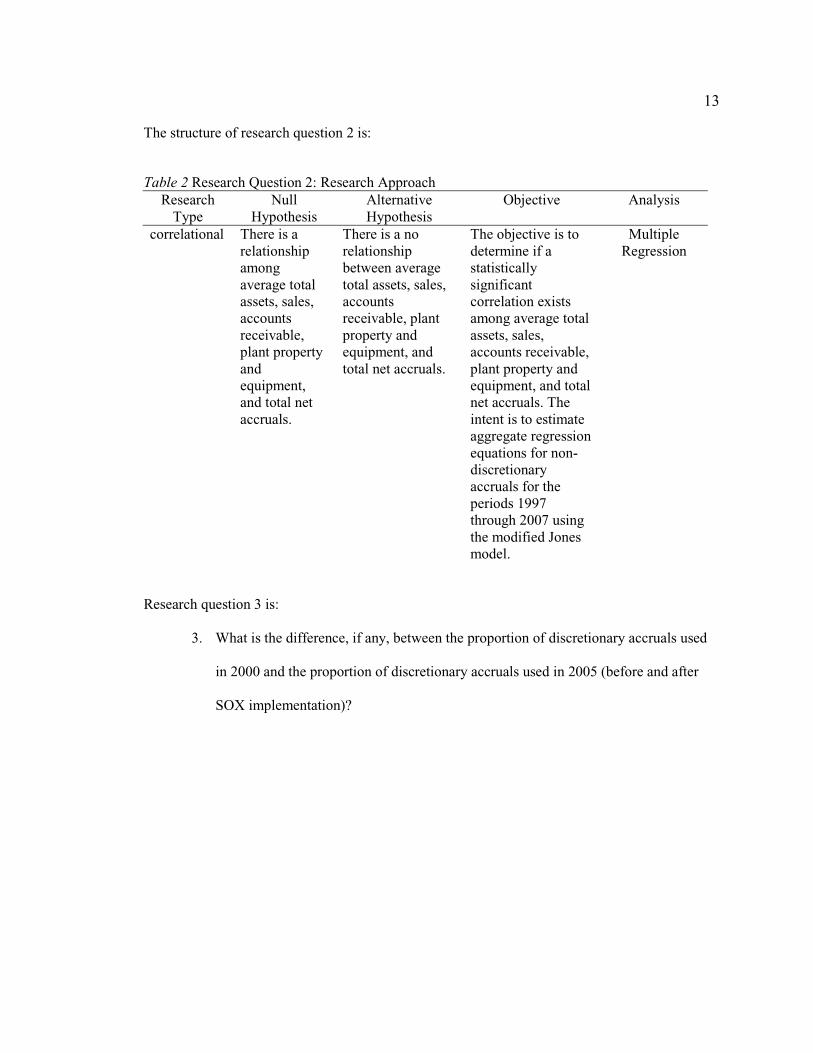
The structure of research question 2 is:
Table 2 Research Question 2: Research Approach Research
Type Null
Hypothesis Alternative Hypothesis
Objective Analysis
correlational There is a relationship among average total assets, sales, accounts receivable, plant property and equipment, and total net accruals.
There is a no relationship between average total assets, sales, accounts receivable, plant property and equipment, and total net accruals.
The objective is to determine if a statistically significant correlation exists among average total assets, sales, accounts receivable, plant property and equipment, and total net accruals. The intent is to estimate aggregate regression equations for non-discretionary accruals for the periods 1997 through 2007 using the modified Jones model.
Multiple Regression
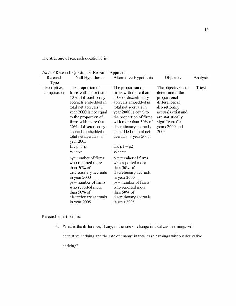
Research question 3 is:
3. What is the difference, if any, between the proportion of discretionary accruals used
in 2000 and the proportion of discretionary accruals used in 2005 (before and after
SOX implementation)?
14
The structure of research question 3 is:
Table 3 Research Question 3: Research Approach Research
Type Null Hypothesis Alternative Hypothesis Objective Analysis
descriptive, comparative
The proportion of firms with more than 50% of discretionary accruals embedded in total net accruals in year 2000 is not equal to the proportion of firms with more than 50% of discretionary accruals embedded in total net accruals in year 2005
The proportion of firms with more than 50% of discretionary accruals embedded in total net accruals in year 2000 is equal to the proportion of firms with more than 50% of discretionary accruals embedded in total net accruals in year 2005.
The objective is to determine if the proportional differences in discretionary accruals exist and are statistically significant for years 2000 and 2005.
T test
H1: p1 p2 H0: p1 = p2 Where: Where: p1= number of firms who reported more than 50% of discretionary accruals in year 2000
p1= number of firms who reported more than 50% of discretionary accruals in year 2000
p2 = number of firms who reported more than 50% of discretionary accruals in year 2005
p2 = number of firms who reported more than 50% of discretionary accruals in year 2005
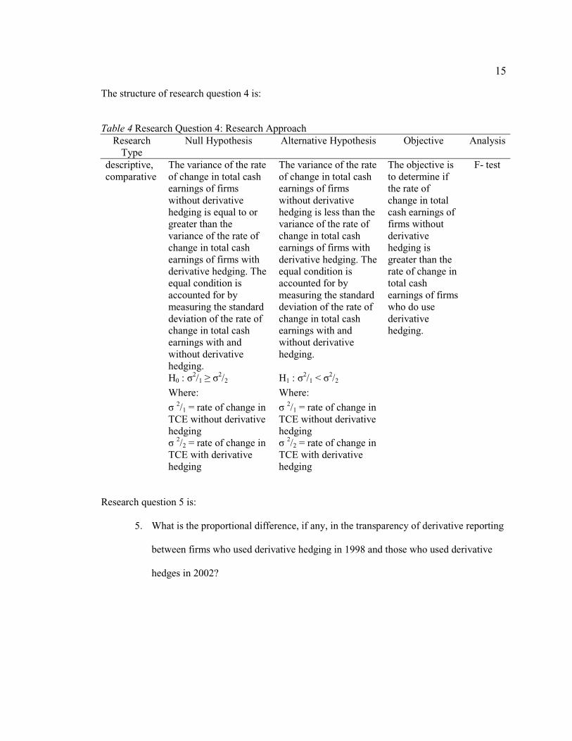
Research question 4 is:
4. What is the difference, if any, in the rate of change in total cash earnings with
derivative hedging and the rate of change in total cash earnings without derivative
hedging?
15
The structure of research question 4 is:
Table 4 Research Question 4: Research ApproachResearch
Type Null Hypothesis Alternative Hypothesis Objective Analysis
descriptive, comparative
The variance of the rate of change in total cash earnings of firms without derivative hedging is equal to or greater than the variance of the rate of change in total cash earnings of firms with derivative hedging. The equal condition is accounted for by measuring the standard deviation of the rate of change in total cash earnings with and without derivative hedging.
The variance of the rate of change in total cash earnings of firms without derivative hedging is less than the variance of the rate of change in total cash earnings of firms with derivative hedging. The equal condition is accounted for by measuring the standard deviation of the rate of change in total cash earnings with and without derivative hedging.
The objective is to determine if the rate of change in total cash earnings of firms without derivative hedging is greater than the rate of change in total cash earnings of firms who do use derivative hedging.
F- test
H0 : 2/1
2/2 H1 : 2/1 < 2/2
Where: Where: 2/1 = rate of change in
TCE without derivative hedging
2/1 = rate of change in TCE without derivative hedging
2/2 = rate of change in TCE with derivative hedging
2/2 = rate of change in TCE with derivative hedging
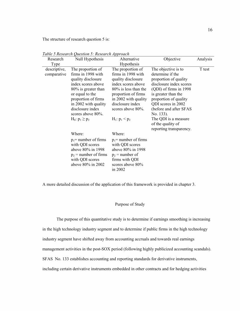
Research question 5 is:
5. What is the proportional difference, if any, in the transparency of derivative reporting
between firms who used derivative hedging in 1998 and those who used derivative
hedges in 2002?
16
The structure of research question 5 is:
Table 5 Research Question 5: Research Approach Research
Type Null Hypothesis Alternative
Hypothesis Objective Analysis
descriptive, comparative
The proportion of firms in 1998 with quality disclosure index scores above 80% is greater than or equal to the proportion of firms in 2002 with quality disclosure index scores above 80%.
The proportion of firms in 1998 with quality disclosure index scores above 80% is less than the proportion of firms in 2002 with quality disclosure index scores above 80%.
The objective is to determine if the proportion of quality disclosure index scores (QDI) of firms in 1998 is greater than the proportion of quality QDI scores in 2002 (before and after SFAS No. 133).
T test
H0: p1 p2 H1: p1 < p2 The QDI is a measure of the quality of reporting transparency.
Where: Where: p1= number of firms with QDI scores above 80% in 1998
p1= number of firms with QDI scores above 80% in 1998
p2 = number of firms with QDI scores above 80% in 2002
p2 = number of firms with QDI scores above 80% in 2002
A more detailed discussion of the application of this framework is provided in chapter 3.
Purpose of Study
The purpose of this quantitative study is to determine if earnings smoothing is increasing
in the high technology industry segment and to determine if public firms in the high technology
industry segment have shifted away from accounting accruals and towards real earnings
management activities in the post-SOX period (following highly publicized accounting scandals).
SFAS No. 133 establishes accounting and reporting standards for derivative instruments,
including certain derivative instruments embedded in other contracts and for hedging activities

17
(Guay, & Kothari, 2003). Released in June 1998, SFAS No.133 represents the culmination of the
US Financial Accounting Standards Board's effort to develop a comprehensive framework for
derivatives and hedge accounting (Hentschel, & Kothari, 1999). The Financial Accounting
Standards Board establishes generally accepted accounting principles for most companies
operating in the United States or requiring financial statements meeting GAAP requirements. The
intent of this regulation is to provide transparency, consistency, and stability to financial reporting
for derivative hedges. The SFAS No. 133 is myriad of layers of amended accounting regulation
and standards (Huang, Ryan, & Wiggins, 2007). The language of SFAS No. 133 allows flexibility
in fair value accounting and some of the regulation dates back to SFAS 52. In this evaluation, an
analysis of derivative hedging activities includes an investigation of transparency in derivative
hedge reporting before and after SFAS No. 133.
Theoretical Framework
The Jones model was created in 1991 by Dechow, Sloan, and Sweeney and modified by
adding the change in receivables in 1995. The modified Jones model is an evaluation
methodology used to segment discretionary accruals from non-discretionary accruals. The model
uses a multiple regression to estimate the non-discretionary accrual proxy and provides a more
robust framework of analysis for measuring accounting accruals. The regression used in the Jones
model references independent variables that have some relationship to non-discretionary accruals.
Normal accruals are driven by sales, PP&E, expected sales growth and current operating
performance, and are used for the independent variables of the Jones model. The model proposes
normal accrual components can be used to predict the non-discretionary component of total
accruals. The difference between total accruals and non-discretionary accruals yields the
discretionary accruals. The intent is to determine how to what degree specific factors in normal
18
accruals influence the level of non-discretionary accruals. The modified Jones model is used in
this evaluation to segment non-discretionary accruals from discretionary accruals for the sample
firms in periods 1997 through 2007.This model has been used by many researchers (Bartov, et.al.,
2001) in the area of earnings management. In 1992, Boynton, Dobbins and Plesko utilized the
modified Jones model and incorporated working capital accruals (Boynton, Dobbins, & Plesko,
1992). In 1999, Navissi used the modified Jones model to evaluate accruals but used a time series
rather than a cross-sectional framework of analysis (Bowman, Navissi, & Burgess, 1991). Many
researchers have referenced the modified Jones model (Subramanyam, 1996; Guay, Kothari, &
Watts, 1996; Collins, & Hribar, 1999; Peasnell, & Pope, 2000; & Gaver, Austin, & Gaver, 1995).
but have altered the independent variables by incorporating factors that reflect cash flow accruals
and working capital such as sales and accounts receivable. In 1994, Hiemstra and Jones used the
modified Jones model to determine if the incremental information content in discretionary
accruals reflects management decisions to smooth earnings.
Earnings management activities during initial public offerings have also been conducted
with the use of a modified Jones model (Roosenboom, Goot, & Mertens, 2003); Shen and Chih
(2005) based the Burgstahler and Dichev (1997), Degeorge, Patel and Zeckhauser (1999) and
Leuz, Nanda and Wysocki (2003) approaches to their studies about the banking sector in 48
countries. In their study, Shen and Chih (2005) calculated the discretionary accruals with three
models. Their first model included 42 countries, the second model included 47 countries and the
last model included 48 countries, all of which revealed discretionary accruals possessed an
average different than zero.
In recent years, accrual models have been used to investigate earnings management
activities in a particular area such as sales and book value of assets (Xie, Davidson, & DaDalt,
2003). Similarly, Myers, Meyers and Omer explored the term of the auditor-client relationship
19
defined by the length of time the auditor spends with the client and used earnings quality in the
dispersion and sign of both the absolute Jones model abnormal accruals and absolute current
accruals as proxies for earnings quality (Myers, Myers, & Omer, 2003). In 2004, Louis and Park
investigated the relationship between earnings management and market performance with the
sales and receivable items, while Shin researched the effect of the board of director's composition
on the earnings management in Canada by using the sales and leverage rate in 2004 (Henock,
2004). Coppens and Peek (2005) researched the earnings management activities by incorporating
variables such as working capital, depreciation, and receivables.
The quality of reporting in financial statements is a major concern for investors,
regulators, and stakeholders. A number of previous studies have investigated the quality of
corporate disclosure as measured by information disclosed in the annual reports and other media
(Imhoff, 1992; Sengupta, 1998; Riahi-Belkaouhi, 2001; Heflin, Shaw & Wild, 2001; & Shaw,
2002). This study also measures transparency and overall quality of reporting by developing an
un-weighted reporting index. All firms who reported the use of derivative hedging are
investigated with an un-weighted scoring index. The results of the scoring are then tested with a
population proportion test to investigate the proportional differences the quality disclosure
reporting of firms in 1998 and 2002 (before and after SFAS No. 133).
Discretionary Accrual Modeling
Although there are many different approaches to estimate this non-discretionary accrual
proxy, estimating the non-discretionary component of accruals typically involves a linear
regression model (Dechow, Sloan & Sweeney, 1995). The first step is to identify the dependent
variable and the independent variables and to determine whether to use a cross-sectional model or

20
a time-series model for the data analysis. For a more detailed explanation of the proposed
research approach, refer to chapter 3.
Definition of Terms
A complete list of definitions and references provided in this section will explain the
meaning of these references. Other references clearly defined in the text are not duplicated in this
section.
Accounting Accrual: the difference between operating earnings and operating cash flow,
which represents the element of earnings subject to management discretion under the generally
accounting principles (GAAP). (Anderson, Caldwell, & Needles, 1994, p.565).
Accounting Actual: the actual value of items sold or purchased by a firm. (Anderson,
Caldwell, & Needles, 1994).
Derivative: a financial contract whose value is derived from the price of another asset
(the underlying asset) (Barton, 2001).
Earnings: the reported earnings before extraordinary items, which represents the earnings
of a firm after all expenses, income taxes, and minority interest, but before preferred dividends,
extraordinary items and discontinued operations (Philbrick & Ricks, 1991).
Earnings Management: an effort “to satisfy consensus earnings estimates and project a
smooth earnings path” (Levitt, 1998). Earnings management is defined in the accounting
literature as “distorting the application of generally accepted accounting principles.” (Dechow et
al., 2003).
Earnings Smoothing: a unique case of earnings management, it tries to make earnings
appear less volatile over time (Dechow et al., 2003). This is consistent with SEC’s definition of
earnings management.

21
Hedging: taking a derivative position that results in a gain (loss) in the contract and a loss
(gain) in the asset or liability. (Barton, 2001).
Operating Cash Flow: the cash generated by the operation of business. (Anderson,
Caldwell, & Needles, 1994).
Operating Earnings: the earnings from continuing operation of the business. (Anderson,
Caldwell, & Needles, 1994,).
Limitations and Delimitations
The high technology industry segment is selected for this study where income
conservatism has been the rule of practice (Kwon, Yin, & Han, 2006). A limitation of this study
is that the inferences and generalizations only apply to the high technology industry segment. In
addition, by restricting the sample to include only U.S. companies, the study inferences and
generalizations are limited to publically traded U.S. companies. Non-profit and government
organizations are outside the scope of this analysis.
Significance of the Study
This research fills the gap in the earnings management literature including the
transparency of financial reporting. This study provides evidence to managers, investors, and
legislators that earning smoothing activities are increasing. The accounting treatment of
operational activities and their impact on the stability of reported earnings in the high technology
industry segment are addressed. Regulations specifically passed by Congress to address
transparency in financial reporting (SOX) and to address derivative hedging (SFAS No. 133) are
investigated. A literature review of research conducted in the area of earnings management is
provided in chapter 2. This research improves upon previous research by studying earnings

22
management without preference to use of accruals or actual transactions. Few studies on earnings
smoothing have focused on actual financial transactions and others on accrual transactions
(Brown, & Caylor, 2005; & Coppens & Peek, 2005); however none have attempted to compare
the two approaches. In addition, the transparency in financial reporting of firms who use
derivative hedging is explored and augments existing literature in the area of earnings
management. The research approach is explained in chapter 3, with the findings in chapter 4, and
the inferences and conclusions in chapter 5.

CHAPTER 2:
LITERATURE REVIEW
Research on earnings management through the use of discretionary accruals and
derivative hedging is the focus of this literature review. In this section, a review of related
research is provided, including an evaluation of existing regulation formulated by FASB. The
strategy used for searching the literature is grounded on the existence of financial regulation
under the Sarbanes-Oxley Act (SOX) and Generally Accepted Accounting Principals (GAAP),
which were created to minimize earnings management activities and to enhance the transparency
in financial reporting. An extensive exploration of discretionary accruals is conducted and
includes an evaluation of peer reviewed research studies that focused on alternative approaches to
earnings management detection and evaluation. The first section of this chapter addresses the
structure of existing financial directives and investigates the financial implications of areas not
addressed with existing regulation. The calculations of accruals are explained and the estimation
of abnormal accruals is evaluated. Derivative hedging and systematic risk is explored and
incentives to hedging against risk are presented. The chapter ends with an evaluation of derivative
hedging under SFAS No. 133 for accounting discretion and the implications to the transparency
in financial reporting for derivative hedging.
The practice of earnings manipulation in financial reporting has existed as long as
financial documents have been used as a tool for evaluation. Earnings management is defined by
the practice of manipulating reported earnings so that the financial peaks and troughs are
smoothed out. In essence, earnings “…do not accurately represent economic earnings at every
point in time” (McKee, 2005, p. 112). Jin (2005) asserted earnings management practices have
always existed.

24
Earnings management is extensively documented in financial literature (Bannister &
Newman, 1996; Beidlerman, 1973; Subramanyam, 1996; Moses, 1987). Collingwood (2001)
examined the intricacies of the earnings smoothing and explored the reasons companies employ
this type of financial manipulation. In this study, Collingwood asserted changes in executive
practices is needed to improve the accuracy of financial reporting.
Review of Related Research
When investors, regulators, and other stakeholders reference financial information of
publically traded firms, they are generally confident that those reported numbers are reliable
(Burgstahler & Dichev, 1997). The reliability of the reported numbers are exposed to a degree of
risk as a result of the discretion allowed in performance modeling and reporting under GAAP
(Gerry, 2003). Burgstahler and Dichev demonstrate the implications of risk exposure in their
1997 study that revealed some managers manage earnings to avoid reporting a loss and to meet
analysts’ expectations. Chaney et al., also illustrates this notion in a study conducted of accruals
and income smoothing published in 1996. As Chaney stated, managers seeking to lower the
perceived risk of the financial stability do so by reducing the variation of inter-period earnings
(earnings smoothing) which in turn reduces the cost of capital for the firm (Chaney, Jeter, &
Lewis, 1998). These practices create artificially inflated stock prices and reduce the number of
price decreases, which signifies financial stability and allows the firm to sell stock at a higher
price. This simulated financial position provides managers justification to collect bonuses and
exercise options (Healy, 1985). Earnings smoothing strategies are also used to stabilize financial
reporting required for government funding and project subsidies (Jones, 1991).
In this section, earnings smoothing through the utilization of discretionary accruals and
derivative hedging is explored. The discretionary accrual section of the literature review includes

25
an examination of the implications of SOX on earnings smoothing and financial reporting. The
accounting treatment of operational activities is also examined by evaluating earning volatility
and stability in financial reporting. The derivative hedging section includes an examination of
hedging practices and implications. This section also includes an examination of the research on
the quality of derivative reporting and the transparency of financial statements.
Discretionary Accruals Activity under SOX
Epps and Guthrie (2007) investigated the material weakness of the Sarbanes-Oxley
Section 404 [SOX 404] that allows managers of firms to manipulate earnings to a greater extent
using discretionary accruals than managers of firms with no SOX 404 material weaknesses. The
Epps and Guthrie study focused on companies that disclosed at least one material weakness in
internal controls within their 2004 SEC filings. In this investigation, the discretionary accruals of
companies with material weaknesses were paired with companies with no reported material
weaknesses during the same period. The focus of the study examined the relationship of reported
SOX 404 weaknesses with the behavior of discretionary accruals for the companies and for
discretionary accruals partitioned by the greatest magnitudes (both positive and negative). The
accruals were then categorized by degree of discretionary accrual performance. The findings
suggested the presence of SOX 404 material weaknesses stimulated a moderate negative effect on
discretionary accruals. However, when the accruals were stratified into high positive, negative,
and low accruals, the overall findings of the research suggests that the existence of material
weaknesses allows for greater manipulation of financial earnings using discretionary accruals
regardless of income increasing or income decreasing (Epps, & Guthrie, 2007).
Cohen, Dey and Lys (2004) evaluated discretionary accruals under SOX regulations in
2004. This analysis revealed an increase in accounting accruals in the two years before SOX and
26
during major financial scandals and a sharp decrease following the issuance of SOX Lobo and
Zhou (2006) reported lower discretionary accruals after SOX than in the period preceding SOX.
In the Lobo and Zhou study, firms incorporated losses more quickly into their earnings in the post
SOX period. This study provided further evidence of the impact of corporate governance on
managers' discretionary accounting decisions. The research findings of the success of SOX in the
minimization of discretionary accrual activities are inconclusive. Specifically, in 2005 Cohen,
Dey, and Lys reported firms engage in less earnings management post-SOX, yet in 2006, Lobo
and Zhou find that firms report earnings more conservatively. However, reporting more
conservatively may be consistent with an increase in earnings management activities
Earnings Management through GAAP Discretions
An example of GAAP discretions can be found in the authorization of varying inventory
models and depreciation schedules. Regulations in these particular areas are vague (Zeff, 2005)
because the language used in these regulations allow for managerial discretion in its’ application
and allow alternative accounting treatment that permits companies to adapt their reporting
methods to reflect their perspective of the firm’s financial position. For example, two companies
experiencing the exact same economic events may use different inventory methods (such as
FIFO, LIFO, or JIT) and depreciation schedules (straight line, step-down, or accelerated) and thus
report different quarterly and annual earnings figures. In addition, under GAAP, firms can choose
alternative methods to account for company performance that result in a distortion of financial
performance (Zeff, 2005). With few exceptions, GAAP requires research and development costs
to be expensed as they are incurred. The costs are reconciled against revenues of the current
period, not against future revenue streams they are formulated to generate. This reporting

27
structure results in understated earnings in current periods and overstated earnings in future
periods (Gerry, 2003).
In 2003, Gerry argued that the GAAP provided discretions for firms to practice earnings
management and in 2003; Tarpley identified patterns of earnings management with a study of 515
earnings management attempts obtained from a survey of 253 auditors. In 2006, Lobo and Zhou
examined changes in discretionary accruals following SOX. In their evaluation, they found that
firms reported lower discretionary accruals after SOX than in the period preceding SOX.
Earnings smoothing is still a common practice and will continue to be as long as value is linked to
earnings stability.
Discretionary Accruals
There is a long history of regulation forged to minimize earnings manipulation and
enhance transparency in financial reporting (Mills, & Newberry, 2001; Wallison, & Hassett,
2004; Zhou, 2007). The interest of analysts, regulators, and investors in general about techniques
that can identify earnings manipulation by the firm’s management has been the focus of existing
financial literature dedicated to earnings management since the early 1970s. Most research
methods focused on the evidence of earnings management rely on the calculation of accounting
accruals and their separation from non-discretionary accruals (Bartov, & Gul, 2001).
Discretionary accruals are considered abnormal or unexpected whereas the non-discretionary
components are considered the expected accrual values stimulated by business cycles (Guay,
Kothari, & Watts, 1996). After the discretionary accrual component is separated, statistical tests
are used to determine if the discretionary accruals of the firm differ from zero, the normal, or
expected value.
28
Despite all the generated interest and abundant literature in earnings management, a
consensus about superiority in the estimation of discretionary accruals does not exist. Guidelines
or axioms about how to estimate these models in order to improve the power of the tests are in
their early stages and there have been few attempts to develop recommendations (Guay, 1995,
Dechow, 1995; Jones, 1991) for evaluation in this area of study. An evaluation of the existing
literature in discretionary accruals is explored.
A New Approach to Evaluating Accruals
Some early attempts to develop standards for analyzing discretionary accruals can be
found in the works of Guay et al (1995) and Dechow et al (1995) and in Young (1999). These
early studies concentrate on models created by Healy in 1985, DeAngelo in 1986, and the Jones
model in 1991. There have been several attempts to account for the relation between accruals and
cash flows such as Hunt in 1997, which augmented the Jones model with the addition of a cash
flow variable (Hunt, Moyer, & Shevlin, 1997).
In 1996, Shivakumar augmented the Jones model by adding five cash flow variables. An
alternative model was introduced in 2000 by Garza-Gómez that was based on cash flow from
operations, which they named the Accounting Process (AP) model. The AP model uses the term
(1/A t-1) as an explanatory variable and is estimated without intercept. The discretionary accrual
component shows a large bias when the (1/A t-1) is used (Garza-Gómez, Okumura, & Kunimura,
2000) and concerns about the methodology of discretionary accruals remains.
Evaluating Abnormal Accruals
Segmenting total accruals into a discretionary and a non-discretionary component is a
difficult task. The discretion exercised by management is unobservable and there are economic
events that stimulate changes in total accruals from one year to the next (Jeter, & Shivakumar,

29
1999). When a researcher estimates discretionary accruals, they are forcing an expectation model
of the expected behavior of accruals in relation to economic events (Kothari, Leone, & Wasley,
2005). Most of the models require the estimation of one or more parameters (Guay, Kothari, &
Watts, 1996). Two methodologies can be found in the literature of earnings management and
accrual evaluation. The time-series approach includes the estimation of parameters for each firm
in the sample by referencing data from periods prior to the current period under review. In
contrast, the cross-sectional approach provides estimates for each period for each firm in the
event sample referencing data of firms in the same industry (Guay, Kothari, & Watts, 1996).
DeChow and Guay utilize the time-series approach in their discretionary accrual
evaluations. The disadvantage of using a time-series approach is that it introduces survivorship
bias as well as selection bias, since the time-series model requires the existence of at least N + 1
years of data (where N is the number of explanatory variables used n the model) (Dechow, Sloan,
& Sweeney, 1995). This limitation inherent in the time-series model reduces the explanatory
power of short series financial data. The time-series approach is effective only when firms in the
sample possess a long series of financial data. Guay requires 15 years of data in their evaluation
of time-series discretionary accruals.
In 1994, Defond and Jiambavolo introduced the cross-sectional method of discretionary
accruals analysis. In this analysis, firms are separated by SIC code and the normal accruals are
estimated using yearly cross sections (DeFond, & Jiambalvo, 1994). The assumption of this
approach is that the situation for each year will affect the firms in the industry in a similar way.
The cross-sectional approach is gaining stability in this area of research and is becoming the
standard approach to estimate accrual models (Dechow, Sloan, & Sweeney, 1995).
In 1996, Subramanyam estimated the Jones model and the modified Jones model
proposed by Dechow et al., (1995) and reported better a fit for the cross-sectional version than for

30
the time-series version of the model (Dechow, Sloan, & Sweeney, 1995). Subramanyam’s
findings suggest the cross-sectional approach generates lower standard errors for the coefficients,
fewer outliers, and coefficients that better fit the predicted signs as measured against the time-
series approach (Shivakumar, 1996). Jeter and Shivakumar also argued in favor of the cross-
sectional estimation method over the time-series approach. Jeter and Shivakumar (1999) contend
industry-relative abnormal accruals can be a useful tool for researchers attempting to detect the
average unconditional earnings management found in the industry.
Discretionary Accrual Modeling
In Jones model introduced in 1991, is a regression-based expectation model that controls
for variations in non-discretionary accruals associated with the depreciation charge as well as
changes in economic activities (Dechow, Sloan, & Sweeney, 1995). The Jones model is
expressed as:
[TAt /At-1] = NDAt = 1(1/At-1) + 1( REVt /At-1) + 2(PPEt /At-1 ) (1)
Where; REVt = change in revenue from period t-1 to t
NDAt = non-discretionary accruals
At = assets
REV = change in revenue
PPEt = gross plant property and equipment
Jones (1991) argued that the change in revenue ( REV) and property plant and
equipment (PPE) terms are used as a control for the non-discretionary component of total accruals
associated with changes in operating activity and level of depreciation. Dechow et al (1995)
31
argued the assumption that all revenue changes in the Jones models are non-discretionary; the
resulting measure of discretionary accruals does not reflect the impact of sales based
manipulation. As a result, Dechow attempted to capture revenue manipulation and altered the
Jones model by subtracting the change in receivables ( REC) from REV for each sample firm.
The modified Jones model becomes:
[TAt/At-1] = NDAt = 1(1/At-1) + 1( REVt/At-1- RECt/At-1) + 2(PPEt/At-1 ) (2)
Calculation of Accruals
The literature to date that focuses on accruals includes two main approaches to calculate the
accrual components of earnings. The balance sheet approach, estimates accruals as:
TAbst = ( CAt - Casht) – ( CLt - STDt)-DEPTNt) (3)
Where; CAt = change in current assets during period t
Cash = change in cash
CLt = change in current liabilities during period t
STDt = the current maturities of long term debt and other short-term debt included in
current liabilities during period t
DEPTNt = depreciation and amortization expense during period t
The total accruals are subtracted from earnings to estimate cash flow from operations (CFOt) as
follows:
CFOt = EBXIt – TAtbs (4)
Where; EBXIt = net income before extraordinary items and discontinued operations
32
TAtbs = total accruals
CFOt = cash flows from operations
The Balance Sheet approach is used to evaluate accruals by DeChow in 1994; Guay, Kothari and
Watts in 1995, and Subramanyam in 1996.
The balance sheet approach to evaluating accrual activity has come under criticism by
Hansen, Collins and Hribar who argue bias is introduced into the estimates of discretionary
accruals under discounted operations, investments and disinvestments in capital expenditures and
other activities that skew the financial statements during the year (Collins, & Hribar, 2000). In
2002, Collins and Hribar introduced an alternative approach to discretionary accrual evaluation.
Under this approach, the researcher can calculate accruals directly from the statement of cash
flows using the formula (Collins, & Hribar, 2002):
TAcf = EBXI – CFOcf (5)
Where; TAcf = the total accrual adjustments provided on the cash flow statement under
the indirect method
EBXI = earnings before extraordinary items and discontinued operations
CFOcf = operating cash flows (from continuing operations) taken directly
This method of calculating accruals by referencing the statement of cash flows is used in this
evaluation of discretionary accruals.
Accrual Modeling and Statistical Distribution Methodology
Prior research on earnings management takes the form of two research designs: those
based on accounting accruals (aggregate accruals, Jones, 1991; or specific accruals, DeGeorge et
33
al., 1999) and those based on the statistical distribution of earnings (Burgstahler, & Dichev,
1997). The first design, also called “accrual model,” and is extensively used in earnings
management literature (Bartov, et.al., 2001). Jones (1991) conducted a study on earnings
management by establishing the normal accruals of a company and comparing them to the actual
accruals reported. The premise behind this evaluation is grounded on the notion that the
difference between discretionary accruals and normal accruals provides the evidence that an
earnings management strategy is employed.
The advantage of this design is that earnings management is easily detected under this
definition of earnings management (Jones, 1991). The disadvantage is that accrual models
(aggregate and specific) lack the theoretical foundation of other statistical models and can not
reliably reflect the exercise of discretion (Nissim, & Penman, 2003). Nissim and Penman (2003),
and Kothari (2005) also claimed that Jones’s and DeGeorge’s models (also called modified Jones
model) could not detect earnings management after SOX. Cohen et al. (2004) found evidence of a
decrease in accruals after the introduction of SOX in 2002 while Lobo and Zhou (2006) examined
changes in discretionary accruals following SOX. The implementation of SOX introduces
significantly greater penalties on CEO/CFOs; therefore, risk adverse managers are likely to be
more conservative in their financial reporting, and report lower discretionary accruals following
SOX (Liu, 2004) Firms with earnings manipulation by excessive accruals also face the risk of
being sued by the SEC. So there are many penalties in place to deter earnings smoothing
however, these regulations do not eliminate earnings smoothing strategies they merely make it
more difficult to identify them. Empirical findings suggest that accruals models that do not
consider long-term earnings growth are potentially undefined and may result in erroneous
inferences about earnings management behavior. This makes it extremely difficult to establish
sound estimates of discretionary accruals that capture discretion exercised by management and it
34
also introduces challenges in evaluating the appropriate research designs for earnings
management research. Collins and Hribar (2000) provided an example of the gap between
empirical procedures and knowledge of the behavior of reported financial statements. The
measurement error in discretionary accrual estimates may lead the researcher to conclude that
earnings management exists when it does not.
The second approach to evaluate earnings management is to examine the statistical
properties of earnings to identify behavior that influences earnings, as developed by Burgstahler
and Dichev (1997) and Degeorge et al., (1999). This is referred to as the Earnings Distribution
Model. Earnings Distribution Models focus on the behavior of earnings around a specified
benchmark, such as zero or a prior quarter's earnings. These types of tests attempt to evaluate
whether the values of cash flows or accruals lie above or below an assigned benchmark and to
determine if they are distributed smoothly and reflect volatility created by the use of management
discretion.
Burgstahler and Dichev (1997) also found volatility in the distribution of reported
earnings around zero and around prior year’s earnings. While Degeorge et al., (1999) used
analyst’s forecasts as a benchmark. Both these studies suggest that if firms had greater incentives
to achieve earnings above a benchmark, then the distribution of earnings after management
publishes the incentives would have fewer observations than expected for earnings amounts just
below the benchmark, and more observations than expected for earnings just above the set
benchmark. Both studies found significantly more observations than expected in the range above
zero earnings, and in the range above the prior period's earnings.
Gore et al. (2001) used 10,000 observations to study the distribution of earnings and
found that fewer companies than expected reported earnings just below zero, and more companies
than expected reported earnings just above zero. Similarly, fewer companies than expected

35
reported earnings just below last year’s figure, and more companies than expected reported
earnings just above last year’s figure. However, it is unclear that this empirically indicates
earnings management strategies are utilized. For example, a firm that reports higher earnings each
year relative to earnings in the prior year would be viewed as a safe firm. On the other hand,
under Gore’s theory; firms that report an increase in earnings in some years and decreases in
others would be viewed as risky. Therefore it could be argued earnings management evaluations
should target earnings decreases exclusively rather than increases in reported numbers.
In 2002, Gore concluded that accruals are a significant part of the earnings management
mechanisms used to boost reported earnings so as to just achieve target (Gore, Pope, & Singh,
2002). The advantage of this method is that researchers can avoid the estimation of discretionary
accruals. The disadvantage is that researchers can not tell the form and magnitude of earnings
management. A noteworthy feature of this design is that the power of this approach comes from
the specificity of their predictions regarding which group of firms will manage earnings, rather
than from a better measure of discretion over earnings (Gore, Pope, & Singh, 2002).
The Earnings Distribution Model is a powerful tool in the earnings management arsenal
in that it identifies contexts in which large numbers of firms appear to manage earnings (Dechow,
Sloan, & Sweeney, 1995). The approach also highlights the frequency of manipulation, though
this rests on an assumption about the distribution of earnings without earnings manipulation.
Myers and Skinner (1999), in the spirit of the Earnings Distribution Model, tested whether the
frequency of increases in consecutive quarterly earnings were greater than would be expected by
chance, and found that it was. In 2008, Allayannis, Roundtree, and Weston conducted an
evaluation of cash flow volatility as valued by investors. The findings of this study are consistent
with a preference by the market for less volatile cash flows and thus, suggesting that managers’

36
efforts to generate smooth financial statements add value, but only through the cash component of
earnings (Allayannis, Rountree, & Weston, 2008).
A study conducted by the University of Illinois at Urbana Champaign (Department of
Accountancy), found a negative relationship between risk aversion and the volatility of earnings
and operating cash flows. In this investigation, CEO incentives to reduce earnings volatility were
explained by the under diversified investment position in their companies’ stock. The risk of
negative valuations inspired the creation of hedging devices to reduce earnings volatility (Abdel-
khalik, 2006).
Direct Cash Flow Earnings Management Methodology
Currently, few studies focus on earnings manipulation via cash flows and real financial
transactions as a means to manage earnings. In 2006, Tucker and Zarowin used a new approach to
breakup earnings into two categories--cash flows and accruals (Tucker, & Zarowin, 2006). In
2006, Tucker and Zarowin measured earnings management activities by evaluating the negative
correlation of the change in accruals with the change in pre-managed earnings. According to
Tucker and Zarowin, the volatility of earnings is the combination of the volatilities of cash flow
and accruals. Under this theory, the following relationship holds:
Var (earnings) = Var (cash flow) + Var (accruals) + 2 Covar (cash flow x accruals) (6)
This formula suggests managers can change the outcome of their reported earnings by either
manipulating the stability of accruals or by altering the level of cash flows (or both) (Tucker, &
Zarowin, 2006). Under these conditions, a firm whose cash flow and earnings are exposed to
interest rate risk can alter their reported earnings by exercising a derivative (cash flow).

37
Derivative Hedging and Systematic Risk
Economic theory explains that the value of equity is equal to the present value of the
expected risk-adjusted dividend, calculated using the risk-free rate of interest. Since interest rate
risk can be hedged by using derivatives, the most important factor that impacts a firm is the value
of future dividends (earnings). Theoretically, higher earnings that are consistently stable will
stimulate dividend growth and increase firm value. Market imperfections increase systematic risk,
which refers to inherent risk in the market and created by the movements of the entire economy
(Emery, & Finnerty, 1997). Systematic risk cannot be diversified away but can be hedged with
financial derivatives (Melumad, Weyns, & Ziv, 1999). If earnings volatility is costly to a firm,
then the firm is faced with incentives to reduce its exposures to risks by reducing the volatilities
of its earnings and may choose to utilize derivative hedges to minimize risk exposure (Emery,
Douglas, & Finnerty, 1997).
Beaver et al. (2000) examined the earnings management incentives of public and private
property and casualty insurance firms, and found that they both avoid losses by using hedging
derivatives. Similarly, Kasznik and McNichols (2002) provided evidence that firms that meet or
beat analysts’ earnings forecasts consistently were valued higher than firms that failed to do so.
Bruns et al., (1990) provided evidence that “…in practice, it appears that a majority of managers
use at least some methods to manage short-term earnings.” (Bruns, & Merchant, 1990).
Derivative Hedging Incentives
DeGeorge et al., (1999) hypothesized that firm managers had various incentives to avoid
reporting a decline in earnings. In fact, the theoretical value of a company’s stock is the present
value of its future earnings and increased earnings represent an increase in shareholder value
38
(Degeorge, Patel, & Zeckhauser, 1999). Beatty et al., (2002) also found that the number of
publicly-held firms reporting continuous increases in earnings per share was unusually high, and
the number was low in privately-held firms. They asserted the cause for this earnings behavior
was the result of required reporting and argued that public firms were more concerned about firm
value, while private firms were more concerned about income tax burdens (Beatty, Ke, & Petroni,
2002). Burgstahler and Eames (2003), Degeorge et al., (1999), and Dechow et al. (2003)
illustrated the same empirical regularity of earnings smoothing however, provided little empirical
evidence to explain this pattern. While Hong and Kyonghee examined management incentives to
smooth earnings (Hong, Keejae & Kyonghee, 2009), Lapointe-Antunes, Magnan, and Gray-
Angers, examined the voluntary disclosure patterns made by Swiss firms with constrains on the
use of discretionary accruals to smooth earnings. In their analysis they explored the effect of
voluntary disclosure on the value relevance of earnings (Lapointe-Antunes, Cormier, Magnan, &
Gray-Angers, 2006).
A survey conducted in 2004 indicated that a majority of firms were willing to forfeit
economic value in exchange for stable earnings (Graham, Harvey, & Rajgopal,
2004).Kirschenheiter and Melumand studied a model of financial reporting where investors infer
the precision of reported earnings. They found reporting a larger earnings surprise reduces the
inferred earnings precision, dampening the impact on firm value of reporting higher earnings, and
providing a natural demand for smoother earnings (Kirschenheiter, & Melumad, 2002). This is
the main force that is driving earnings management practice of managers.
Liu and Yao (2003) asserted that the market value was higher for earnings-stable stocks
than for earnings-volatile stocks. Based on their sample firms, from 1985 to 2000, earnings-stable
stocks significantly outperformed earnings-volatile stocks in returns (Liu, & Yao, 2003). McKee
(2005) claimed that firms with lower earnings volatility were being valued higher than the firms

39
with higher earnings volatility (McKee, 2005). However, given the current market and the
inherent volatility and consumer uncertainty, Collingwood asserted there is no financial benefit
for earnings smoothing (Collingwood, 2001).
Derivative Hedging
The use of financial derivatives is widespread, particularly among large publicly traded
firms. Derivatives are to speculate or to hedge against risk (Emery, & Finnerty, 1997). As
described in chapter 1, this study is concerned with hedging rather than speculating with
derivatives however it is important to note that derivative contracts are used for speculating
purposes as well as hedging against risk. Derivative transactions, because of their complex and
obscure nature, attract attention from regulators, accounting standard setters and researchers.
(Naor, 2006).
In most cases, large firms are the predominant users of derivatives (Mian, 1996). In 1996,
Mian proved that firm size was positively correlated to derivative use (as firm size increased, so
did the use of derivatives). In a survey of the Wharton School, Bodnar and Günther found that
German firms are more likely to use derivatives than US firms, with 78% of German firms using
derivatives compared to 57% of US firms. However, the financial markets are international and
foreign currency derivative hedging can affect domestic firms that trade in these markets (Bodnar,
& Gebhardt, 1998). In this survey, almost half of the respondents considered stable cash flows
and earnings stability their primary objective.
In 2005, McKee argued the reduction of earnings volatility may be the goal of many
firms and minimized the need for total earnings volatility elimination (McKee, 2005). It is
conceivable that if derivatives can reduce risk, they are also useful in stabilizing earnings trends.
For example, if a firm is faced with a variable-interest rate on a debt obligation, and a financial

40
manager believes that interest rates will increase in the next quarter, the manager may consider
hedging this interest rate with an interest rate swap. To hedge the floating rate exposures, the
manager can enter into a pay-fixed receive-variable interest rate swap, which will stabilize
reported earnings simply by exercising a hedging derivative (Singh, 2004). Guay conducted a
study to evaluate the role of derivatives in firms initiating derivatives use. The results are
consistent with firms using derivatives to hedge (Guay, 1999), and minimize entity risk.
Bodnar, Hayt, and Marston (1998), explored selective hedging in their study conducted in
1998. In this study, Bodnar, Hayt, and Marston found 66 percent of the firms in their sample
timed their interest rate hedges based on their perception of anticipated interest rate volatility in
the market (Bodnar, & Gebhardt, 1998).
Based on McKee’s study conducted in 2005, derivatives offer many opportunities to
manage earnings because firms are free to exercise discretion in the timing of derivative contracts
(McKee, 2005). As explained above, the timing of a derivative option contract provides an
opportunity to manage earnings by timing when a contract that will be exercised as well as
reducing the risk being hedged or un-hedged. Barton (2001) claimed that firms with recorded
derivative use were more likely to engage in earnings management than companies without
reported derivative use (p.24).
While all these papers provide evidence that the use of derivatives is consistent with
incentives to hedge a firm against associated risk (Bodnar, et.al., 1998), none of these papers
directly test whether the use of derivatives reduces earnings volatilities resulting in smoother
earnings.

41
Derivatives and SFAS No.133 Accounting Discretion
To prove that derivative use captures basic attributes of hedging, Barton (2001) used the
correlation between the notional amount and the hedge ratios. He also provided evidence that
suggested that derivative users tend to have less volatile operating cash flows and total accruals
than nonusers (Barton, 2001). In 2002, Pincus and Rajgopal concluded that managers of oil and
gas producing firms first established the extent to which they would use derivatives to hedge
commodity volatility and then managed earnings volatility by trading off discretionary accruals
and hedging to smooth earnings (Pincus, & Rajgopal, 2002). While their results showed no
evidence that the extent of hedging was a significant determinant of hedging, they did find
however that the extent of hedging was a considerable building block for earnings management
strategies.
Nissim and Penman (2003) proved that firm value was positively related to earnings and
inversely related to interest rates. According to Stulz (1996), a derivative is the most powerful
tool in reducing interest costs (Nissim, & Penman, 2003). Stulz pointed out that hedging
increased firm value only if managers believed they had informational advantages. Stulz (1996)
embraced behavioral finance in his conclusions—an area still in its infancy phase of academic
finance.
Earnings Management with Derivative Hedging
Derivative hedging involves taking a financial position that results in a gain or a loss to
offset a loss or gain in the underlying asset or liability being hedged (Stulz, 2003). Hedging will
reduce the volatility of a firm's earnings by trading off potential gains against potential losses.
42
Therefore, it can be argued that derivatives provide an effective and efficient means to reduce
cash flow and earnings volatility (Stulz, 2003).
Hedging is a common practice among public firms. Huang, Ryan and Wiggins contend
managers are risk averse. In their study of the use of nonlinear derivatives (options), they found
nonlinear cash flow characteristics in investment opportunity, debt, and executive compensation
all relate positively to nonlinear derivative usage (Huang, Ryan, & Wiggins, 2007). It is logical
therefore, that the reduction in risk exposure would be desirable by all risk-averse stakeholders. In
2009, Minton, Stulz, and Williamson conducted a study to examine the use of credit derivatives
by US bank holding companies with assets in excess of one billion dollars from 1999 to 2005.
They found that in 2005 the gross notional amount of credit derivatives held by banks exceeds the
amount of loans on their books. Their research confirmed only 23 large banks out of 395 used
credit derivatives and most of their derivatives positions are held for dealer activities rather than
for hedging of loans. They contend the findings suggest that the use of credit derivatives by banks
to hedge loans is limited by the adverse selection and moral hazard problems and because of the
inability of banks to use hedge accounting when hedging with credit derivatives. This study raises
important questions about the extent to which the use of credit derivatives provides financial
stability in the banking industry. (Minton, Stulz, & Williamson, 2009)
Hedging the fair value of assets and liabilities is a financially fundamental process that
one could define as simple in application (Emery, Douglas, & Finnerty, 1997). The assumptions
used in the models created for the fair value calculations introduce complexity. The complexity in
derivative hedging models begin with the imbedded assumptions that (a) markets are efficient, (b)
behavioral financial factors are irrelevant, (c) asset returns are normally distributed random
variables, (d) volatility can be stabilized, (e) prices follow a normal distribution, (f) investors are
risk averse (g) return on investment is directly related to risk exposure, and (h) transaction costs
43
are excluded (Guay, 1999). Hedging cash flows is more difficult to accomplish because the cash
flow and the hedging derivatives are changing at different rates (Myers, & Skinner, 1999). In
addition, most derivative contracts have no market reference because they are not actively traded
in the secondary market and as a result, the hedge is not always completely effective.
It is important to note, derivatives and other innovative financial maneuvering serve
legitimate business and investment objectives (Guay, 1999). The ability to shift, replace, or
transfer risks with financial derivatives is an essential tool for today’s businesses. However,
derivatives also present a number of serious challenges for the entire financial reporting system
regardless of industry sector (Sheedy, 1997). Although derivatives have been used for many
years, the way in which they are used today is new; complex; and somewhat vague in their
application (Guay, 1999). As a result, detecting earnings management through the manipulation
of derivatives is difficult to identify. (McKee, 2005). Tucker (2006) contends exercising a
hedging derivative targeted at interest rate risk, a firm can minimize the exposure to interest rate
volatility and decrease the interest rate cost while decreasing its cash flow (by capturing the cost
associated with exercising the hedging derivative).
By timing the utilization of hedging derivatives, a firm can alter their current earnings
(Tucker, & Zarowin, 2006). For example, suppose managers of a firm believe additional earnings
are needed on the financials to meet pre-determined targets. Under this scenario, a manager can
terminate a hedging derivative that carries an unrealized gain. Then, according to the GAAP
rules, the unrealized gain will be added to current earnings immediately--thus increase earnings.
On the other hand, suppose the manager believes it is necessary to reduce earnings on reported
financials, under this scenario a manager can terminate a hedging derivative that carries an
unrealized loss. Terminating a financial derivative can result in a stop of payment streams under
the derivative contract, thus reducing reported earnings (Tucker, & Zarowin, 2006).

44
Disclosure Quality of Derivative Reporting
The transparency in financial reporting and the disclosure quality of derivative hedging is
a major concern for stakeholders and regulators. Since 1990, the Financial Accounting Standards
Board (FASB) has issued seven accounting pronouncements pertaining to financial instruments.
The approach employed by FASB has been to issue addendums to existing regulation and piece
together a complete reporting regulation package (Blankey, & Schroeder, 2000). The
development of the regulation for derivative instruments under SFAS No. 133 has taken the
FASB 10 years to complete. Prior to the issuance of SFAS No. 133, the FASB issued SFAS No.
119 Disclosure about Derivative Financial Instruments and Fair Value of Financial Instruments.
The intent of SFAS No. 119 is to improve the previous standards. In 2000, the FASB issued
SFAS No. 138 as an amendment to SFAS No. 133 and is to be used when certain technical
changes from SFAS No. 133 are introduced (Tombley, 2003). Prior studies have been conducted
to investigate disclosure quality associated with derivative hedging such as Sengupta in 1998,
Blankey & Schroeder in 2000, and Riahi-Belkaouhi in 2001. Prior studies indicate a correlation
exists between disclosure quality and firm specific characteristics.
In a study conducted by Ashmed and Courtis, an association between quality disclosure
in financial reporting and firm specific characteristics has been to explanatory variables from the
research on agency costs, political costs, corporate governance and information asymmetry
(Ahmed, & Courtis, 1999). Lobo and Zhou examined the relationship between earnings
management and disclosure quality in 2001. This evaluation is focused on identifying the
relationship between (a) information asymmetry and disclosure quality and (b) earnings
management and information asymmetry (Lobo, & Zhou, 2001).

45
Malone, Fries, and Jones examined the association between the extent of corporate
disclosure with firm specific characteristics within the oil and gas industry. In this study, a
weighted disclosure index is created by referencing industry analysts’ reports for the associated
weights (Malone, Fries, & Jones, 1993). The analysts were asked to weight 129 factors according
to the relative importance of each factor in the overall investment decision. The total actual scores
of the index were reported as a percentage of total possible scores. The findings suggest firms
listed on major stock exchanges with high debt-to-equity ratios report more financial information
if they have a larger number of shareholders.

CHAPTER 3:
RESEARCH METHOD
In this chapter, the research design and approach are explained and the setting and sample
is provided. The treatment used to evaluate the five research questions is described and the data
collection and analysis is defined. The measures taken for the protection of participants’ rights are
summarized and the chapter ends with a summary of the topics explained.
The focus of this study is on earnings management through the utilization of derivative
hedges and accounting treatment of operational activities of a firm in the high technology
industry segment. The main question is whether the accounting methodology affects the firm’s
ability to smooth earnings and if earnings management through the use of discretionary accruals
has decreased after the issuance of SOX. The quality of disclosure and financial transparency in
reporting of derivative hedging is addressed by the creation of a disclosure quality index to
investigate transparency in derivative reporting before and after SFAS No. 133.
The purpose of the analysis in the accounting treatment of operational activities is to
evaluate the differences between the properties of accrual earnings and cash earnings in such a
way as to clarify the different ways in which the accounting treatment of operational activities
may account for any differences in earnings smoothing. In much of the literature on earnings
smoothing, it is assumed that accruals are used to manage earnings (Bartov, et. al., 2001).
However, Nissim and Penman (2003) claimed that after the implementation of SOX, accrual
models have become ineffective in the detection of earnings smoothing. As Cohen, Dey, and Lys
(2005) contend, firms use actual transactions rather than accruals in earnings smoothing.

47
Research Design and Approach
The high tech industry segment is selected for this study to maximize the opportunity to
investigate firms engaged in income conservatism, since these types of firms confront greater
risks of shareholder litigation than other industries (Lobo, Zhou, 2006). High tech industry
companies are also affected to a greater degree by conservative accounting standards on research
and development costs (Uday, Wasley, & Waymire, 2004). Conservatism defined as the higher
verification standard applied to favorable information that results in lower cumulative earnings
and net assets (Watts, 2003). The presence of income conservatism is materialized in significantly
higher proportions of losses and lower average profitability levels for technology firms relative to
non-technology firms (Kwon, Yin, & Han, 2006). These differences arise primarily from
differences in operating cash flow levels attributable to R&D expenses. Technology firms also
show evidence of more negative non-operating accruals (Uday, Wasley, & Waymire, 2004).
The data mining process included online data retrieval from the published financial
reports of high technology firms for the years 1997 – 2007. The Mergent database was used to
extract data files for each company randomly selected for the sample. Only U.S. firms were
included in the study and all dollar values were converted into millions for consistency in
comparison. The total cash earnings and the total net accruals were determined with adjustments
to the raw reported financial statements explained in chapter 1 (Anderson, Caldwell, & Needles,
1994). Data was collected, descriptive statistics are explained and graphical depictions of total
cash earnings, and total net accruals are provided. An aggregate t test of all years ranging from
1997 to 2007 is conducted to test the difference in means between total cash earnings and total
net accruals.
The modified Jones model is referenced to separate discretionary accruals from non-
discretionary accruals. The process includes the implementation of a linear regression model
48
where the independent variables are identified with a proxy for non-discretionary accruals. The
proxy is created by categorizing total accruals into non-discretionary and discretionary accruals.
The non-discretionary component reflects business conditions (such as firm growth and length of
the operating cycle) that create and destroy accruals, while the discretionary component
highlights management choices (Jones, 1991). After the cross-sectional discretionary accruals are
identified for all firms for the years 1997 – 2007, a test of proportion means is conducted using a
binomial distribution to test the proportion of discretionary accruals in 2000 with discretionary
accruals in 2005. The intent of this investigation is to evaluate the proportion of discretionary
accrual activities before and after SOX implementation (SOX was implemented in 2002).
The modified Jones model is employed by regressing accrual data from many firms in the
same industry for a single time period (cross-sectional) or by regressing accrual data from the
same firm across several time periods (time-series). There are disadvantages to both methods but
the cross-sectional analysis is considered a better method for the following technical reasons:
1. Time-series analysis may not have enough observations in the estimation period to
obtain reliable parameter estimates for a linear regression.
2. The coefficient estimates on Sales and GPPE may not be stationary over time.
3. The self-reversing property of accruals may result in serially correlated residuals.
Since the coefficient estimates on the change in sales and gross property plant and
equipment are not stationary over time, it is impossible to make valid statistical inferences from
the linear regression results obtained with time-series analysis (Nissim, & Penman, 2003).
Because making valid statistical inferences is paramount in this study, the cross-sectional
approach is used.
49
Cross-Sectional Analysis
The cross-sectional model used in this evaluation requires a two-stage process for
calculations. To accomplish this, the results from the first part of the analysis are used in the next
stage of analysis to reach the needed estimate (Peasnell, & Pope, 2000). To estimate the non-
discretionary accrual amounts, firm-specific amounts for each independent variable are used for a
particular period across several different firms. In essence, each data item [(TNA), (ATA), (
Sales – Rec), and (GPPE)] is coming from the same period with the next data set originating
from a different firm. The data set of 30 different firms with accounting data for the year ending
2007 yields one estimated regression equation. Since the period range in this study is from 1997
to 2007, ten regression equations are estimated for the 30 firms—one for each fiscal year.
The difference in the rate of change in total cash earnings with derivative hedging and the
rate of change in total cash earnings without derivative hedging is investigated with an F test.
Two groups are created for this analysis. One group includes the calculated rate of change of total
cash earnings of firms who did not report the use of derivative hedging during the period 1997 to
2007 and the other group includes the calculated rate of change in total cash earnings of firms
who did report the use of derivative hedging during the period 1997 to 2007. The rate of change
for all firms is aggregated across 10 years and the F test is used to investigate the variances in the
rate of change of both groups. The difference in the quality of derivative reporting of firms who
reported the use of derivative hedging is evaluated by aggregating un-weighted index scores of
quality disclosure for the periods 1997 to 2007. All companies who reported the use of derivative
hedging in their annual reports are evaluated. The focus of this test is on the quality of financial
statements and annual reports and is based on accounting policy information, anticipated hedging
activities, risk assessment, and net fair value information. All firms who reported the use of
derivative hedging are evaluated in these 4 areas of reporting transparency. Each area of

50
transparency contains a select number of questions (policy information = 4 questions; anticipated
hedging activities = 5 questions; risk assessment = 3 questions; and net fair value = 7 questions).
Each firm is scored a 1 for reporting and a 0 if otherwise. Then all scores are summed and divided
by the possible score. For example, the risk area includes 3 questions so a firm could score a 3 if
they reported in each area and in which case, 3 would be divided by the 3 (possible score)
resulting in a total score of 1. The objective is to yield one quality disclosure score for all firms.
After descriptive depictions of each individual quality factor is presented for all derivative
hedging firms, each individual firm score is summed and divided by the possible score of 4
(policy information, anticipated hedging activities, risk assessment and net fair value). For
example if a firm scored a 3 out of the possible 4 in the transparency test (Risk, Accounting,
Hedging, and Fair Value) then the 3 is divided by 4 (3/4 = .75) resulting in a .75 overall quality
disclosure score ( referenced as QDI score from this point on). The final QDI scores of all firms
who reported derivative hedging in 1998 and 2002 is investigated with a population proportion
test. The intent is to evaluate the proportion of QDI scores of firms who reported the use of
derivative hedging before and after the implementation of SFAS No. 133.
Setting and Sample
In the later half of 2001, the U.S. financial market experienced crashes and frauds of
Enron, WorldCom and other companies that required the U.S. Congress to regulate corporate
governance. These financial crises were addressed with the Congressional issuance of the
Sarbanes-Oxley Act of 2002, which attempted to restore confidence in the securities markets
(Ribstein, 2002). A study of the mitigating effects of the SOX Act conducted by Aono and Guan
(2007) found earnings manipulative behavior to round earnings result in an upward bias. Early
findings are inconclusive on the success of the Act (Zhou, 2007). Cohen, Dey and Lys (2004)
51
asserted firms engage in less earnings management post-SOX, but Lobo and Zhou (2006) find
that firms report earnings more conservatively. Reporting more conservatively could be
consistent with greater earnings management Cohen, Dey, & Lys, (2004). In the high tech
industry, companies are affected to a significant degree by conservative accounting standards
such as SFAS 2 on R&D costs (Uday, Wasley, & Waymire, 2004).
The Statement of Financial Accounting Standard No. 133 passed in 1998, established
accounting and reporting standards for derivative instruments and hedging activities (Wallison, &
Hassett, 2004). The decision to use derivatives for hedging is contigent on existing exposure
factors (i.e. foreign sales and foreign trade) and on variables associated with theories of optimal
hedging (i.e., size and R&D expenditures). In addition, the level of derivatives used depends only
on a firm's exposure through foreign sales and trade (Allayannis, & Ofek, 1997). Empirical
evidence suggests that managers are averse to reporting earnings volatility introduced by SFAS
133 (Barton, 2001). From these findings, it is evident that firms seeking to smooth earnings
volatility have been using discretionary accruals and or derivative hedging (Barnes, 2003). Data
were randomly drawn from listings of all U.S. companies traded on U.S. markets. The high
technology industry segment is the target of this study due to income conservatism
characteristics. The high technology segment drawn for the sample is defined by SIC (Standard
Industrial Classification) codes which refer to a four-digit number assigned to U.S. industries and
their products. The specific SIC codes used in this analysis can be found in Table 6 in Appendix
A. All firms classified by these SIC codes are drawn and thirty companies are randomly drawn
from to form the sample. The simple random sample is generated by listing all firms in the
sample in Microsoft Excel and using the rand function to generate 30 random companies. If a
company in the sample has not reported financials for the entire period under review (1997 –
2007) they are dropped from the sample and another firm from the population described by SIC

52
code is randomly selected to yield 30 companies in the sample. Annually reported data is used for
all calculations and dollar values of all firms are translated into millions. The significance level
for all tests in this study is set to .05.
The sample size is 30 the Type I and Type II errors are analyzed to ensure sampling error
is not introduced in this study as a result of a small sample size. A sample size of 30 is selected
due to the arduous research involved in the analysis of these firms for the period 1997 through
2007. Figure 1 in Appendix B reports the Type I and Type II errors.
The observed effect size (Cohen's d) defined as the difference between two means
divided by a standard deviation for the data is used to measures the observed difference and is
also used to analyze the meaning of the data (the larger the effect, the more meaningful). The d is
defined as the difference between two means divided by the pooled standard deviation for those
means. In Figure 1, the Type I error reflects the level of significance for testing. In this analysis,
all tests are evaluated with a level of significance of .05. The Type II errors are measured by beta.
The Type II errors are all below the standard .20 (Cohen, 1992). The measured effects are
medium to large. The Type I and Type II errors for the linear regression analysis are presented in
Figure 2 within Appendix B:
The Type II errors are low and the thresholds for the Cohen’s d are large for all periods.
The post-hoc statistical power of the regression models are strong. The R2 which measures the
model are all high (68% or higher) indicating the model effectively fits the data.
Treatment
Research question 1 is measured by using an aggregate approach to calculate the total
cash earnings and the total net accruals of all the firms in the sample. The total net accruals are

53
calculated to investigate the difference in earnings volatility between total net accruals and total
cash earnings, the total cash earnings is calculated as:
TCE = ( C – CI – STK + EI) (7)
Where: TCE = total cash earnings
C = change in cash
CI = cash dividends
STK = stock repurchases
EI = equity issuance
The total net accruals are calculated:
TNA = NI – C – CI – STK + EI (8)
Where: TNA = total net accruals
NI = net income
C = change in cash
CI = cash dividends
STK = stock repurchases
EI = equity issuance
Research Question 1
An aggregate t test of all years ranging from 1997 to 2007 is conducted to test the
difference in means between total cash earnings and total net accruals. The objective is to
investigate the difference in the means of reported numbers in total net accruals and total cash
earnings. In theory, total cash earnings minus total net accruals should equal zero (Anderson,
Caldwell, & Needles, 1994). However, accruals are used to reduce timing and mismatching
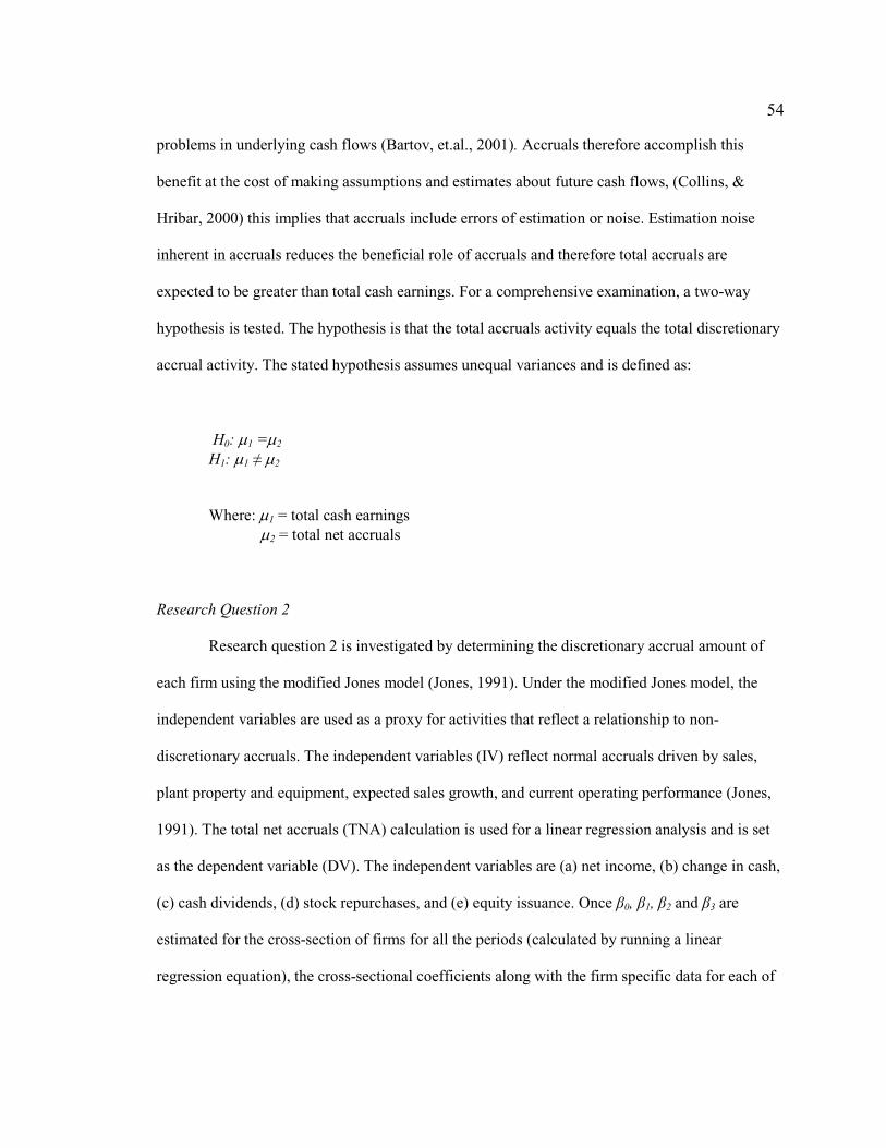
54
problems in underlying cash flows (Bartov, et.al., 2001). Accruals therefore accomplish this
benefit at the cost of making assumptions and estimates about future cash flows, (Collins, &
Hribar, 2000) this implies that accruals include errors of estimation or noise. Estimation noise
inherent in accruals reduces the beneficial role of accruals and therefore total accruals are
expected to be greater than total cash earnings. For a comprehensive examination, a two-way
hypothesis is tested. The hypothesis is that the total accruals activity equals the total discretionary
accrual activity. The stated hypothesis assumes unequal variances and is defined as:
H0: 1 = 2
H1: 1 2
Where: 1 = total cash earnings 2 = total net accruals
Research Question 2
Research question 2 is investigated by determining the discretionary accrual amount of
each firm using the modified Jones model (Jones, 1991). Under the modified Jones model, the
independent variables are used as a proxy for activities that reflect a relationship to non-
discretionary accruals. The independent variables (IV) reflect normal accruals driven by sales,
plant property and equipment, expected sales growth, and current operating performance (Jones,
1991). The total net accruals (TNA) calculation is used for a linear regression analysis and is set
as the dependent variable (DV). The independent variables are (a) net income, (b) change in cash,
(c) cash dividends, (d) stock repurchases, and (e) equity issuance. Once 0, 1, 2 and 3 are
estimated for the cross-section of firms for all the periods (calculated by running a linear
regression equation), the cross-sectional coefficients along with the firm specific data for each of
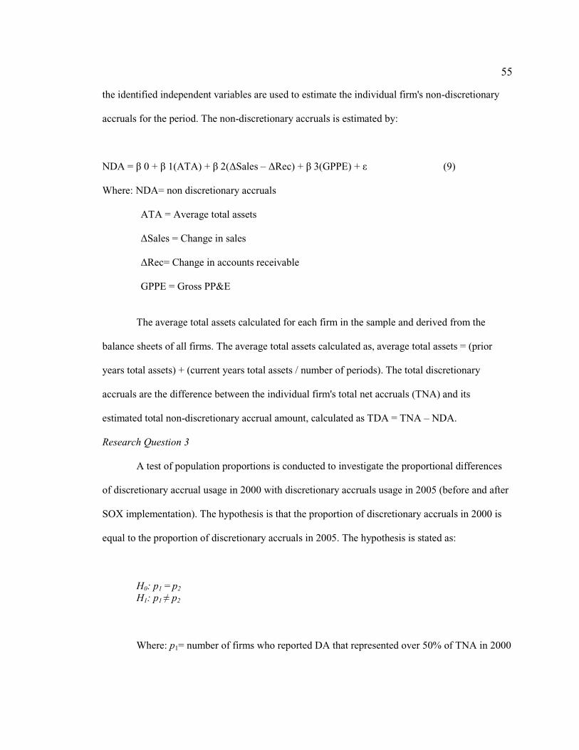
55
the identified independent variables are used to estimate the individual firm's non-discretionary
accruals for the period. The non-discretionary accruals is estimated by:
NDA = 0 + 1(ATA) + 2( Sales – Rec) + 3(GPPE) + (9)
Where: NDA= non discretionary accruals
ATA = Average total assets
Sales = Change in sales
Rec= Change in accounts receivable
GPPE = Gross PP&E
The average total assets calculated for each firm in the sample and derived from the
balance sheets of all firms. The average total assets calculated as, average total assets = (prior
years total assets) + (current years total assets / number of periods). The total discretionary
accruals are the difference between the individual firm's total net accruals (TNA) and its
estimated total non-discretionary accrual amount, calculated as TDA = TNA – NDA.
Research Question 3
A test of population proportions is conducted to investigate the proportional differences
of discretionary accrual usage in 2000 with discretionary accruals usage in 2005 (before and after
SOX implementation). The hypothesis is that the proportion of discretionary accruals in 2000 is
equal to the proportion of discretionary accruals in 2005. The hypothesis is stated as:
H0: p1 = p2
H1: p1 p2
Where: p1= number of firms who reported DA that represented over 50% of TNA in 2000
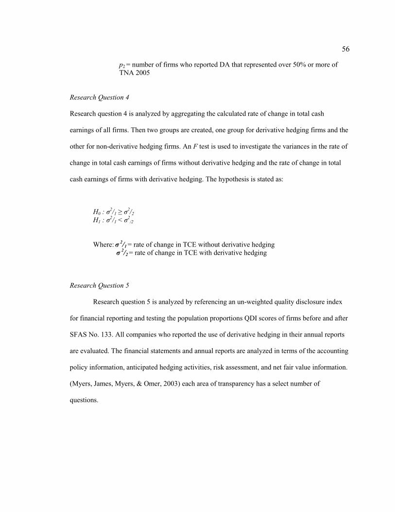
56
p2 = number of firms who reported DA that represented over 50% or more of TNA 2005
Research Question 4
Research question 4 is analyzed by aggregating the calculated rate of change in total cash
earnings of all firms. Then two groups are created, one group for derivative hedging firms and the
other for non-derivative hedging firms. An F test is used to investigate the variances in the rate of
change in total cash earnings of firms without derivative hedging and the rate of change in total
cash earnings of firms with derivative hedging. The hypothesis is stated as:
H0 : 2/1
2/2
H1 : 2/1 < 2
/2
Where: 2/1 = rate of change in TCE without derivative hedging 2/2 = rate of change in TCE with derivative hedging
Research Question 5
Research question 5 is analyzed by referencing an un-weighted quality disclosure index
for financial reporting and testing the population proportions QDI scores of firms before and after
SFAS No. 133. All companies who reported the use of derivative hedging in their annual reports
are evaluated. The financial statements and annual reports are analyzed in terms of the accounting
policy information, anticipated hedging activities, risk assessment, and net fair value information.
(Myers, James, Myers, & Omer, 2003) each area of transparency has a select number of
questions.

57
Policy Information Questions
1. Are the accounting policies and the method adopted explained in the financial statements or annual reports?
2. Are the uncertainties of future cash flows explained? 3. Are the objectives for holding or issuing derivative financial instruments explained? 4. Are the objectives for holding or issuing derivative financial instruments explained?
Figure 3. This figure shoes the index scoring for policy information. All firms are assigned a “1” for providing the data in their financial statements or annual reports and a “0” if otherwise. The depth of policy information reported is not included in the scoring index. This scoring is only concerned with whether the firm reported this information or not.
Hedges of Anticipated Transactions
1. Is a description of the anticipated hedging transaction provided?
2. Is a description of the period until the hedge is expected to occur reported in the financial statements or annual reports?
3. Is a description of the hedging instrument reported?
4. Is the amount of any deferred or un-recognized gain or loss reported? 5. Is the expected timing of recognition as revenue or expense reported?
Figure 4. This figure shoes the index scoring for hedges of anticipated transactions. All firms are assigned a “1” for providing the data in their financial statements or annual reports and a “0” if otherwise. The depth of anticipated hedging transaction information reported is not included in the scoring index. This scoring is only concerned with whether the firm reported this information or not.

58
Risk Information
1. Are the contractual re-pricing or maturity dates for interest rate risk reported?
2. Are the effective interest rates or weighted averages reported?
3. Are the maximum amounts of credit risk exposure at the reporting date provided?
Figure 5. This figure shows the index scoring for risk information. All firms are assigned a “1” for providing the data in their financial statements or annual reports and a “0” if otherwise. The depth of risk reported information is not included in the scoring index. This scoring is only concerned with whether the firm reported this information or not.
Net Fair Value Information
1. Are the aggregate net fair values of the reporting date provided? 2. Does the reporting show separately in aggregate net fair value of those financial assets or financial liabilities, which are not readily traded on organized markets?
3. Is the method used for determining net fair value explained? 4. Are any significant assumptions made in the determination of net fair value provided? 5. Is the carrying amount and the net fair value of either the individual asset or appropriate groupings of those individual assets reported?
6. Are the reasons for not reducing the carrying amount provided? 7. Is the nature of the evidence that provides the basis for management’s belief that the carrying amount will be recovered explained?
Figure 6. This figure shows the index scoring for net fair value. All firms are assigned a “1” for providing the data in their financial statements or annual reports and a “0” if otherwise. The depth of net fair value information reported is not included in the scoring index. This scoring is only concerned with whether the firm reported this information or not.

59
Disclosure Quality Policy
Information Questions
Hedges of Anticipated Transactions
Risk Information
Net Fair Value
Information
Total Possible Scores
Total Disclosure
Quality Score
1 or 0 Score 1 or 0 Score 1 or 0 Score 1 or 0 Score 4 Scores
Sum of Scores divided by possible scores
Figure 7. This figure shows the scoring for QDI scores. All firms are assigned a “1” for providing the data in their financial statements or annual reports and a “0” if otherwise. The depth of reported information in each disclosure quality category is not included in the scoring index. This disclosure quality index is only concerned with whether the firm reported this information or not.
After each firm is scored a 1 for reporting and a 0 if otherwise, all scores are summed and
divided by the possible score (for example the Risk area includes 3 questions so a firm could
score a 3 if they reported in each area so if they scored a 3 then the 3 would be divided by the 3
(possible score) resulting in a 1). Under this scoring, all reporting is ranked and ranges from 0 to
1 with 0 equal to poor quality disclosure in financial reporting and 1 equal to superior quality
disclosure in financial reporting. Only 1 score of disclosure quality is needed to test the
population proportion so the measure is used again by summing up all final scores for each area
of transparency and dividing by the possible score. Then the population proportion of the final
quality disclosure scores of all firms who reported derivative hedging in 1998 and 2002 are
evaluated. The hypothesis is that the proportion of the QDI scores above 80% in 1998 is greater
than the proportion of the QDI scores above 80% in 2002. The hypothesis is stated as:
H0: p1 p2
H1: p1 < p2
Where: p1= number of firms with QDI scores above 80% in 1998 p2 = number of firms with QDI scores above 80% in 2002
60
Instrumentation and Materials
In research question 1, an aggregate t test of all years ranging from 1997 to 2007 is
conducted to test the difference in means between total cash earnings and total net accruals. The
objective is to investigate the difference in the means of total net accruals and total cash earnings
for all years. The hypothesis is that the means of accounting accruals is equal to the means of
cash earnings for all firms. This is a comparative research question and is investigated with
inferential statistics. This test is a parametric test and the data is ratio scaled.
In research question 2 is a correlational evaluation and is conducted to generate a more
robust framework of analysis for total accruals. This is a comparative study that includes
correlational analysis of, discretionary accruals that are segmented away from non-discretionary
accruals (Kothari, Leone, & Wasley, 2005). To accomplish this separation, the modified Jones
model introduced in 1991 is used. The modified Jones model is a multiple linear regression model
that regresses the total net accruals to estimate the coefficients for discretionary accruals once a
cross-sectional or a time-series approach has been established (Hribar, & Collings, 2002; Kothari,
Leone, & Wasley, 2005, & Tucker, & Zarowin, 2006). This is a correlational analysis and is a
descriptive analysis. The data is ratio scaled. This is a parametric analysis that takes the form of a
linear multiple regressions. In this analysis, there are 4 independent variables that are continuous
(average total assets, change in sales, change in accounts receivable, gross plant property and
equipment), and one dependent variable (TNA) that lie on a continuum. Each independent
variable is obtained from the published annual financial statements of each firm in the sample.
The total net accrual (TNA) is calculated from the total net accruals equation while NDA is
determined with the regression of total net accruals. This regression correlational analysis is used
to determine the discretionary component of total accruals.

61
Research question 3 is a comparative test conducted to evaluate the proportion of
discretionary accruals used before and after the issuance of SOX. Once the discretionary
components are determined for each firm in the sample for all periods 1997 – 2007 in research
question 2, a test of population proportions is conducted to investigate the proportion of
discretionary accruals utilized before and after the implementation of the SOX Act. This is a
parametric test and the data used in this investigation is ratio scaled. The hypothesis is that the
proportion of discretionary accruals is less before the issuance of SOX than it is after.
Research question 4 is a comparative test to investigate the rate of change in total cash
earnings with derivative hedging and the rate of change in total cash earnings without derivative
hedging. This F test is a parametric test and the data in is ratio scaled. In this test, the hypothesis
is that the rate of change in total cash earnings of firms with derivative use is be less volatile than
the rate of change in total cash earnings of firms without derivative use. The focus of this test is
on the volatility of earnings and an F test for equality of two population variances is performed to
determine if the standard deviations of two populations are equal (in this case, the rate of change
in total cash earnings with derivative hedging and the rate of change in total cash earnings
without derivative hedging).
Research question 5 is a comparative research question and is addressed with inferential
statistics. The data is ordinal scaled. An un-weighted quality disclosure index is created to
evaluate firms who reported the use of derivative hedging in four categories of financial
transparency (Risk, Hedging, Fair Value, and Accounting). Each area of transparency has a select
number of questions and each firm is scored a 1 for reporting and a 0 if otherwise. Although it
seems as though nominal data is used, these scores are used to rank the quality of disclosure (0 to
1) and are ordinal in nature. A test of population proportions is then conducted to investigate the
62
proportional differences between quality disclosure in financial reporting before and after the
implementation of SFAS No. 133. This population proportion test is a parametric statistical test.
Measures Taken for the Protection of Participants’ Rights
The data used in this investigation is derived from publically published financial reports
submitted to the Securities and Exchange Commission. All data is pulled by SIC code, saved to a
password protected file, and ordered by company ticker code number. No human subjects were
used in this research study.
Summary
The data used in this research is obtained from public financial data and is accessed using
Mergent Online database. The financial statements and annual reports of the firms in the sample
are analyzed to determine the difference in means of total cash earnings and total net accruals.
The financial statements include, (a) balance sheets, (b) income statements, (c) statements of cash
flows, (d) statements of retained earnings and (e) annual reports. Discretionary accruals are
separated from total accruals for all years 1997 – 2007 using a cross-sectional modified Jones
model. The proportions of discretionary accrual usage are investigated with a test of population
proportions before and after the issuance of the SOX Act. The rate of change in total cash
earnings with derivative hedging is tested against the rate of change in total cash earnings without
derivative hedging using an F test to investigate the differences in variances. The quality of
disclosed derivative hedging is analyzed by an un-weighted quality transparency index. The
quality of disclosure in derivative hedging is then tested with a population proportion test to
investigate financial reporting before and after SFAS No. 133.

63
CHAPTER 4:
RESULTS
The findings of the evaluations are provided in this section. The statistical test summaries
are included in the Appendix and the interpretations of findings and recommendations are
provided in chapter 5. The impact to positive social change in the area of financial management is
explained in chapter 5.
The economic crisis that began during the late 20th century resulted in dramatic losses in
equity values within international financial markets. Between June 2007 and November 2008,
Americans lost more than one quarter of their net worth. By early November 2008, the S&P 500
was down 45 percent from its 2007 high. Housing prices had dropped 20% from their 2006 peak,
with futures markets signaling a 30-35% potential drop. Total home equity in the United States,
which was valued at $13 trillion at its peak in 2006, had dropped to $8.8 trillion by mid-2008, and
was still falling in late 2008. Total retirement assets, Americans' second-largest household asset,
dropped by 22 percent, from $10.3 trillion in 2006 to $8 trillion in mid-2008. During the same
period, savings and investment assets (apart from retirement savings) lost $1.2 trillion and
pension assets lost $1.3 trillion. Taken together, these losses total $8.3 trillion (Minton, Stulz, &
Williamson, 2009). The crisis of the financial system has resulted in a crisis in the entire
economical system (Minton, Stulz, & Williamson, 2009). It has been argued by Crutchley,
Jensen, and Marshal (2007) that this financial anomaly is a full market correction directly
attributable to the lack of international regulation and consistency in domestic regulation
standards within financial markets.
One of the most significant factors in financial markets that have lead to this economic
convergence is rooted in the lack of reporting requirements for derivative hedging and
speculating (Huddart & Louis, 2008). Derivatives are off the balance sheet items and are not
65
reported in the same manner as other assets and liabilities (Barton, & Simko, 2002). In addition,
these financial instruments have no true value reference and do not accurately reflect market
value (Hentschel & Kothari, 1999). Therefore, any unreported gains or losses not reflected in
published financial statements or annual reports cannot be captured with the use of the modified
Jones model or the quality disclosure index are excluded from this study. In this chapter, the
results of the quantitative analysis are reported. The instrumentation, data preparation, statistical
analysis, and summary of the findings are provided in this section.
Problems Encountered
Only firms that published complete financial information for the entire period 1997
through 2007 are included. Two firms (ticker codes MXIM and JDSU) are excluded from the
sample because they do not possess financial information for the entire period under review. Two
firms (ticker codes LSCC and CTXS) are randomly drawn from the population to yield a sample
of 30 firms.
Quantitative Data Analysis
As described in chapter 3, this study is designed to investigate the impact of the
accounting treatment on earnings smoothing and to evaluate the impact of derivative hedging on
real cash earnings. The transparency of derivative reporting has also been investigated to explore
the disclosure quality of derivative hedging. There is an established, literature-based need for
understanding in the presence of regulation, earnings smoothing through the use of discretionary
accruals and derivative hedging. The theoretical foundations of this study employed a systematic,
analysis-based study, utilizing the modified Jones model and a quality disclosure index
(Lapointe-Antunes, Cormier, Magnan, & Gray-Angers, 2006), similar to the index used by
66
Lapointe –Antunes to measure the relationship between voluntary disclosure, earnings smoothing,
and the value-relevance of earnings.
Total Cash Earnings and Total Net Accruals
Research question 1 is a comparative investigation conducted to addresses the impact of
accounting treatment on reported earnings. Generally speaking, total cash earnings should equal
total net accruals. In empirical data, accruals use estimates to help reduce timing and mismatching
problems in underlying cash flows. The overall benefit of accruals is achieved at the cost of
making assumptions and estimates about future cash flows. As a result, accruals possess a
fundamental estimation error. Since the errors in estimation reduce the beneficial role of accruals,
they should be more volatile than real earnings. To examine this relationship, total cash earnings
and total cash accruals are calculated for all firms using an aggregate testing approach for periods
1997 to 2007. The statements of cash flows of the firms are referenced to calculate the total cash
earnings for all the firms in the sample for years 1997 through 2007 using the following formula:
TCE = Cash + Cash Dividends + Stock Repurchases – Equity Issuances (10)
The total net accruals are calculated for all firms using the following formula:
TNA = Net Income – TCE (11)
The average total cash earnings are significantly greater than the average total net accruals as
depicted in Figure 2 located in Appendix C.

67
Figure 8. Average total cash earnings and average total net accruals: 1997 – 2007
An, aggregate evaluation and t test is conducted for all firms in the sample during periods
1997 through 2007. The hypothesis:
H0 : 1 2
H1 : 1 2
Where: 1 = average total cash earnings 2 = average total net accruals
The test is conducted as a two-way t test. The results of the aggregate t tests for all years
1997 through 2007 depicted in table 8 provide the aggregate results of the t test. The null
hypothesis that total cash earnings are equal to total net accruals is rejected and is statistically
significant for all years. These results are provided in table 8. In addition, a t test for all years
1997 through 2007 is conducted to test the sensitivity of the aggregate t tests. The result of the
sensitivity t test for all years is also statistically significant.
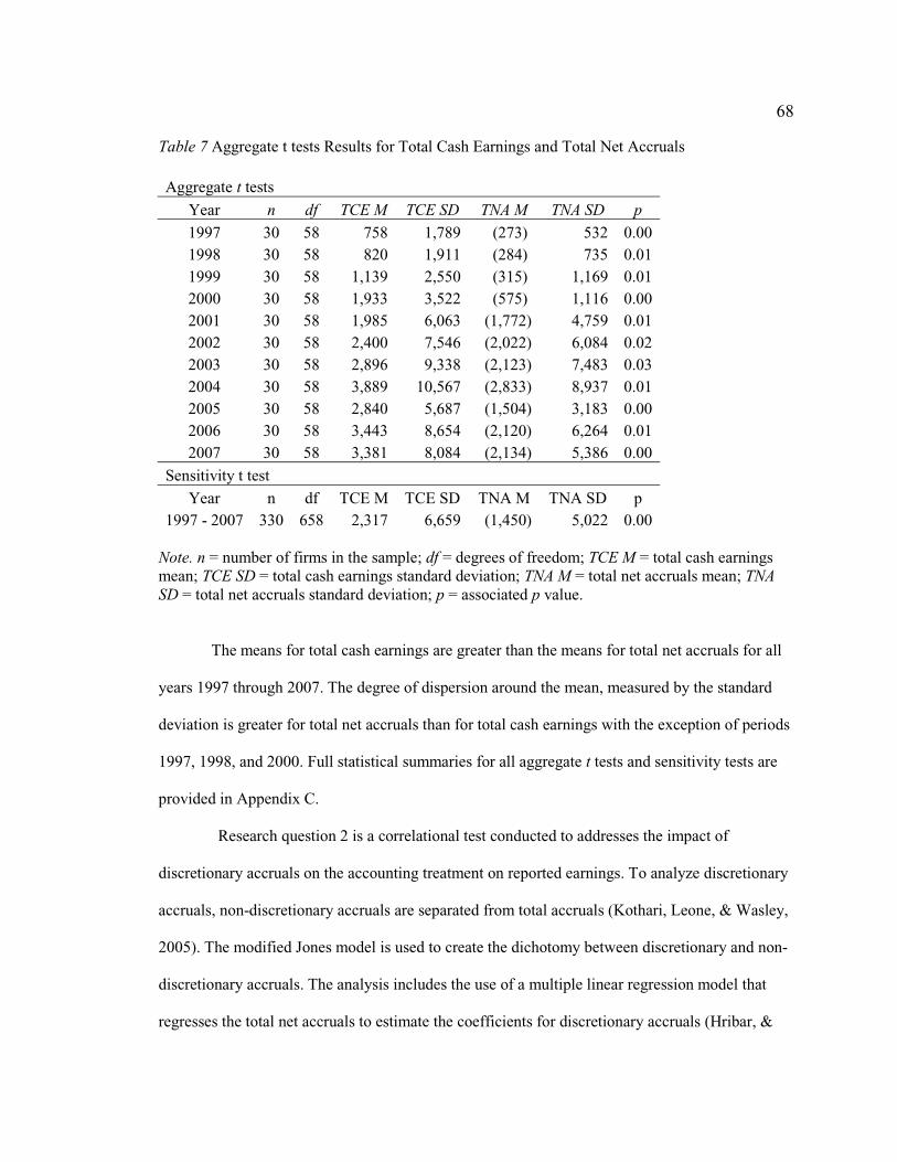
68
Table 7 Aggregate t tests Results for Total Cash Earnings and Total Net Accruals
Aggregate t tests
Year n df TCE M TCE SD TNA M TNA SD p
1997 30 58 758 1,789 (273) 532 0.001998 30 58 820 1,911 (284) 735 0.011999 30 58 1,139 2,550 (315) 1,169 0.012000 30 58 1,933 3,522 (575) 1,116 0.002001 30 58 1,985 6,063 (1,772) 4,759 0.012002 30 58 2,400 7,546 (2,022) 6,084 0.022003 30 58 2,896 9,338 (2,123) 7,483 0.032004 30 58 3,889 10,567 (2,833) 8,937 0.012005 30 58 2,840 5,687 (1,504) 3,183 0.002006 30 58 3,443 8,654 (2,120) 6,264 0.012007 30 58 3,381 8,084 (2,134) 5,386 0.00
Sensitivity t test
Year n df TCE M TCE SD TNA M TNA SD p 1997 - 2007 330 658 2,317 6,659 (1,450) 5,022 0.00
Note. n = number of firms in the sample; df = degrees of freedom; TCE M = total cash earnings mean; TCE SD = total cash earnings standard deviation; TNA M = total net accruals mean; TNA SD = total net accruals standard deviation; p = associated p value.
The means for total cash earnings are greater than the means for total net accruals for all
years 1997 through 2007. The degree of dispersion around the mean, measured by the standard
deviation is greater for total net accruals than for total cash earnings with the exception of periods
1997, 1998, and 2000. Full statistical summaries for all aggregate t tests and sensitivity tests are
provided in Appendix C.
Research question 2 is a correlational test conducted to addresses the impact of
discretionary accruals on the accounting treatment on reported earnings. To analyze discretionary
accruals, non-discretionary accruals are separated from total accruals (Kothari, Leone, & Wasley,
2005). The modified Jones model is used to create the dichotomy between discretionary and non-
discretionary accruals. The analysis includes the use of a multiple linear regression model that
regresses the total net accruals to estimate the coefficients for discretionary accruals (Hribar, &
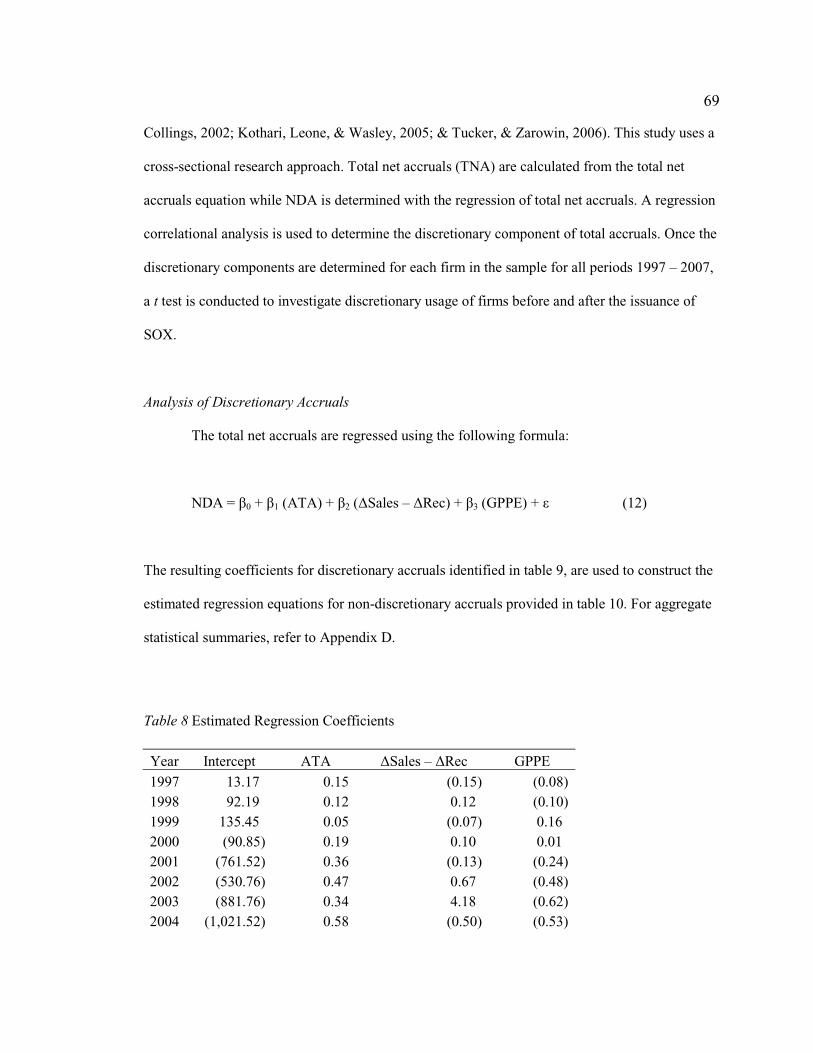
69
Collings, 2002; Kothari, Leone, & Wasley, 2005; & Tucker, & Zarowin, 2006). This study uses a
cross-sectional research approach. Total net accruals (TNA) are calculated from the total net
accruals equation while NDA is determined with the regression of total net accruals. A regression
correlational analysis is used to determine the discretionary component of total accruals. Once the
discretionary components are determined for each firm in the sample for all periods 1997 – 2007,
a t test is conducted to investigate discretionary usage of firms before and after the issuance of
SOX.
Analysis of Discretionary Accruals
The total net accruals are regressed using the following formula:
NDA = 0 + 1 (ATA) + 2 ( Sales – Rec) + 3 (GPPE) + (12)
The resulting coefficients for discretionary accruals identified in table 9, are used to construct the
estimated regression equations for non-discretionary accruals provided in table 10. For aggregate
statistical summaries, refer to Appendix D.
Table 8 Estimated Regression Coefficients
Year Intercept ATA Sales – Rec GPPE
1997 13.17 0.15 (0.15) (0.08)1998 92.19 0.12 0.12 (0.10)1999 135.45 0.05 (0.07) 0.16 2000 (90.85) 0.19 0.10 0.01 2001 (761.52) 0.36 (0.13) (0.24)2002 (530.76) 0.47 0.67 (0.48)2003 (881.76) 0.34 4.18 (0.62)2004 (1,021.52) 0.58 (0.50) (0.53)

70
2005 77.50 0.20 (0.32) (0.11)2006 (1,226.39) 0.45 (0.31) (0.44)2007 376.67 (1.27) 3.23 (0.05)
Note. The table shows the regression coefficients for the aggregate non-discretionary accruals for periods 1997 through 2007.
Table 9 Estimated Regression Equations
Year Estimated Regression Equation R2Adjusted
R2
1997 = 13.168+ 0.147x - 0.148x - 0.079x 0.82 0.80
1998 = 92.193 + 0.122x + 0.124x - 0.102x 0.70 0.66
1999 = 135.452 + 0.045x - 0.066x + 0.161x 0.88 0.87
2000 = -90.851 + 0.189x + 0.101x + 0.012x 0.83 0.81
2001 = -761.518 + 0.358x - 0.130x - 0.238x 0.73 0.70
2002 = -530.757+ 0.472x + 0.674x - 0.483x 0.86 0.84
2003 = -881.759 + 0.343x + 4.176x - 0.618x 0.86 0.84
2004 = -1,021.520 + 0.584x - 0.504x - 0.528x 0.91 0.90
2005 = 77.502 + 0.196x - 0.315x - 0.113x 0.83 0.82
2006 = -1,226.387 + 0.447x - 0.306x - 0.435x 0.80 0.78
2007 = 376.669- 1.272x + 3.225x - 0.049x 0.68 0.64
Note. In a multiple linear regression model, the adjusted R2 measures the proportion of the variation in the dependent variable accounted for by the explanatory variables. Unlike r square, the adjusted R2 allows for the degrees of freedom associated with the sums of the squares. Therefore, even though the residual sum of squares decreases or remains the same as new explanatory variables are added, the residual variance does not. The adjusted R2 is generally considered a more accurate goodness-of-fit measure than R2; nevertheless, both the R2 and the adjusted R2 are reported in this table (Aczel, & Sounderpandian, 2002).
The adjusted R2 for each year are above .80 with the exception of year 2001 (.70), and
2007(.64). The adjusted R2 allows for the degrees of freedom associated with the sums of the
squares. Therefore, even though the residual sum of squares decrease or remain the same as new
explanatory variables are added, the residual variance does not. For this reason, the adjusted R2 is
considered an accurate goodness-of-fit measure and this linear regression was used on the
assumption that the independent variables possess strong explanatory power. These equations

71
were used to predict the aggregate non-discretionary accruals of all firms for periods 1997 –
2007. The cross-sectional coefficients along with a specific firm's data are used to estimate the
firm specific non-discretionary accruals for the period 1997 through 2007.
Discretionary Accruals Activity
Discretionary accruals have steadily increased from 1997 to 2007. Figure 2 provides a
visual depiction of discretionary and non-discretionary accrual activities for this period.
Figure 9. Total accrual activity years: 1997 - 2007
As illustrated by the histogram of total accruals, the discretionary accruals represent a significant
portion of total accruals. A breakout of total net accruals is provided in Table 11. For full
statistical summaries, refer to Appendix D.
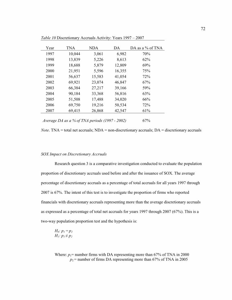
72
Table 10 Discretionary Accruals Activity: Years 1997 – 2007
Year TNA NDA DA DA as a % of TNA
1997 10,044 3,061 6,982 70% 1998 13,839 5,226 8,613 62% 1999 18,688 5,879 12,809 69% 2000 21,951 5,596 16,355 75% 2001 56,637 15,583 41,054 72% 2002 69,921 23,074 46,847 67% 2003 66,384 27,217 39,166 59% 2004 90,184 33,368 56,816 63% 2005 51,508 17,488 34,020 66% 2006 69,750 19,216 50,534 72% 2007 69,415 26,868 42,547 61%
Average DA as a % of TNA periods (1997 - 2002) 67%
Note. TNA = total net accruals; NDA = non-discretionary accruals; DA = discretionary accruals
SOX Impact on Discretionary Accruals
Research question 3 is a comparative investigation conducted to evaluate the population
proportion of discretionary accruals used before and after the issuance of SOX. The average
percentage of discretionary accruals as a percentage of total accruals for all years 1997 through
2007 is 67%. The intent of this test is to investigate the proportion of firms who reported
financials with discretionary accruals representing more than the average discretionary accruals
as expressed as a percentage of total net accruals for years 1997 through 2007 (67%). This is a
two-way population proportion test and the hypothesis is:
H0: p1 = p2
H1: p1 p2
Where: p1= number firms with DA representing more than 67% of TNA in 2000 p2 = number of firms DA representing more than 67% of TNA in 2005
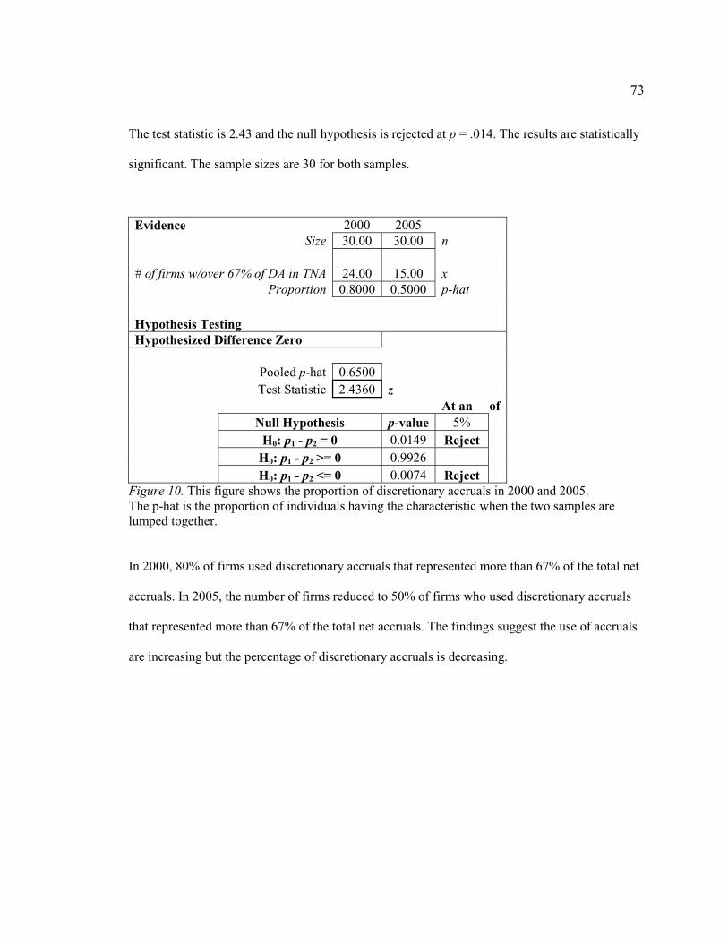
73
The test statistic is 2.43 and the null hypothesis is rejected at p = .014. The results are statistically
significant. The sample sizes are 30 for both samples.
Evidence 2000 2005 Size 30.00 30.00 n
# of firms w/over 67% of DA in TNA 24.00 15.00 x Proportion 0.8000 0.5000 p-hat
Hypothesis Testing Hypothesized Difference Zero Pooled p-hat 0.6500 Test Statistic 2.4360 z At an � of Null Hypothesis p-value 5% H0: p1 - p2 = 0 0.0149 Reject H0: p1 - p2 >= 0 0.9926 H0: p1 - p2 <= 0 0.0074 Reject
Figure 10. This figure shows the proportion of discretionary accruals in 2000 and 2005. The p-hat is the proportion of individuals having the characteristic when the two samples are lumped together.
In 2000, 80% of firms used discretionary accruals that represented more than 67% of the total net
accruals. In 2005, the number of firms reduced to 50% of firms who used discretionary accruals
that represented more than 67% of the total net accruals. The findings suggest the use of accruals
are increasing but the percentage of discretionary accruals is decreasing.
74
Figure 11. Discretionary Accrual Usage: Year 2000
Figure 12. Discretionary Accrual Usage: Year 2005
Discretionary accruals represented 75% of total net accruals in year 2000 and 66% in 2005. The
use of discretionary accruals has decreased 12% from year 2000 to 2005 for high technology
firms.
75
Analysis of Derivative Hedging
Research question 4 is a comparative investigation conducted to analyze the variance of
the rate of change in total cash earnings of firms who use derivative hedging and compare these
earnings to firms who do not use derivative hedging. Using an aggregate analysis approach, the
rate of change in total cash earnings is calculated across 10 years (using the rate of change
calculation reduces the sample size from 11 to 10) and an F test is conducted to evaluate the rate
of change in total cash earnings with derivative hedging against the rate of change in total cash
earnings without derivative hedging. The expectation is that the rate of change in total cash
earnings with derivative hedging is less than the rate of change in total cash earnings without
derivative hedging. The stated hypothesis is:
H0 : 2/1
2/2
H1 : 2/1< 2
/2
Where: 2/1 = rate of change in total cash earnings without derivative hedging 2/2 = rate of change in total cash earnings with derivative hedging
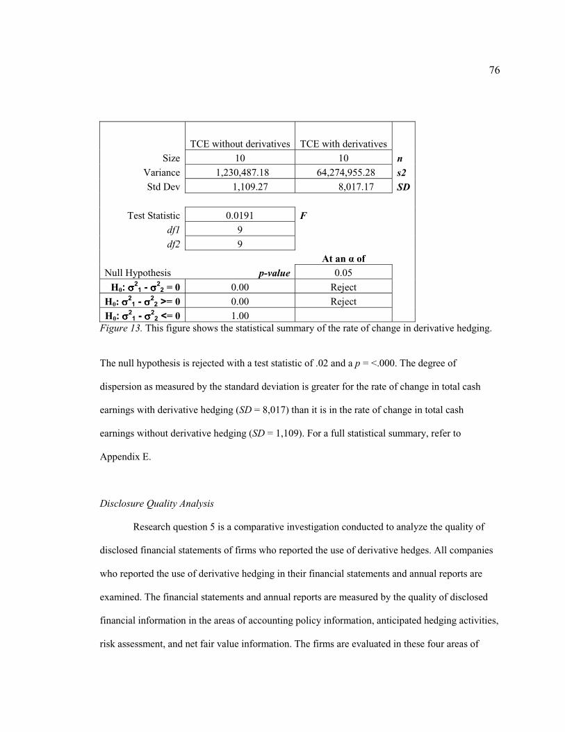
76
TCE without derivatives TCE with derivatives
Size 10 10 n Variance 1,230,487.18 64,274,955.28 s2 Std Dev 1,109.27 8,017.17 SD
Test Statistic 0.0191 F df1 9
df2 9
At an of Null Hypothesis p-value 0.05
H0: 21 -
22 = 0 0.00 Reject
H0:21 -
22 >= 0 0.00 Reject
H0: 21 -
22 <= 0 1.00
Figure 13. This figure shows the statistical summary of the rate of change in derivative hedging.
The null hypothesis is rejected with a test statistic of .02 and a p = <.000. The degree of
dispersion as measured by the standard deviation is greater for the rate of change in total cash
earnings with derivative hedging (SD = 8,017) than it is in the rate of change in total cash
earnings without derivative hedging (SD = 1,109). For a full statistical summary, refer to
Appendix E.
Disclosure Quality Analysis
Research question 5 is a comparative investigation conducted to analyze the quality of
disclosed financial statements of firms who reported the use of derivative hedges. All companies
who reported the use of derivative hedging in their financial statements and annual reports are
examined. The financial statements and annual reports are measured by the quality of disclosed
financial information in the areas of accounting policy information, anticipated hedging activities,
risk assessment, and net fair value information. The firms are evaluated in these four areas of

77
transparency (Risk, Hedging, Fair Value, and Accounting). Each area of transparency has a select
number of questions. Each firm is scored a “1” for reporting the information and a “0” if
otherwise. Then all scores are summed and divided by the possible score (for example the Risk
area includes 3 questions so a firm could score a 3 if they reported in each area. If they score a 3
then the 3 would be divided by the 3 (possible score) resulting in a 1). The averages of disclosed
quality scores have been determined for all firms who reported the use of derivative hedging for
the periods 1997 through 2007.
Table 11 Average QDI Scores: Years 1997 - 2007
Year Policy
Information
Hedges of Anticipated Transactions
Risk Information
Net Fair Value Information
Disclosure Quality
1997 0.81 0.65 0.73 0.63 0.70 1998 0.77 0.62 0.63 0.56 0.65 1999 0.81 0.62 0.65 0.59 0.67 2000 0.80 0.64 0.78 0.63 0.71 2001 0.88 0.67 0.76 0.69 0.75 2002 0.90 0.75 0.87 0.71 0.81 2003 0.88 0.72 0.79 0.68 0.77 2004 0.90 0.71 0.81 0.68 0.78 2005 0.93 0.74 0.86 0.67 0.80 2006 0.94 0.80 0.86 0.71 0.83 2007 0.90 0.75 0.87 0.71 0.81
Note. A score of 1 = superior disclosure quality in financial reporting and a score of 0 = poor disclosure quality in financial reporting.
There is some volatility in the QDI scores for firms who reported derivative hedging.
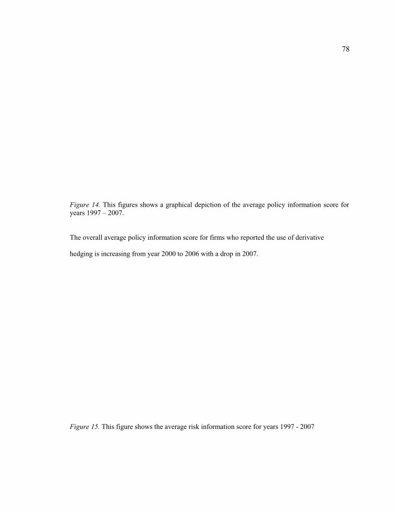
78
Figure 14. This figures shows a graphical depiction of the average policy information score for years 1997 – 2007.
The overall average policy information score for firms who reported the use of derivative
hedging is increasing from year 2000 to 2006 with a drop in 2007.
Figure 15. This figure shows the average risk information score for years 1997 - 2007
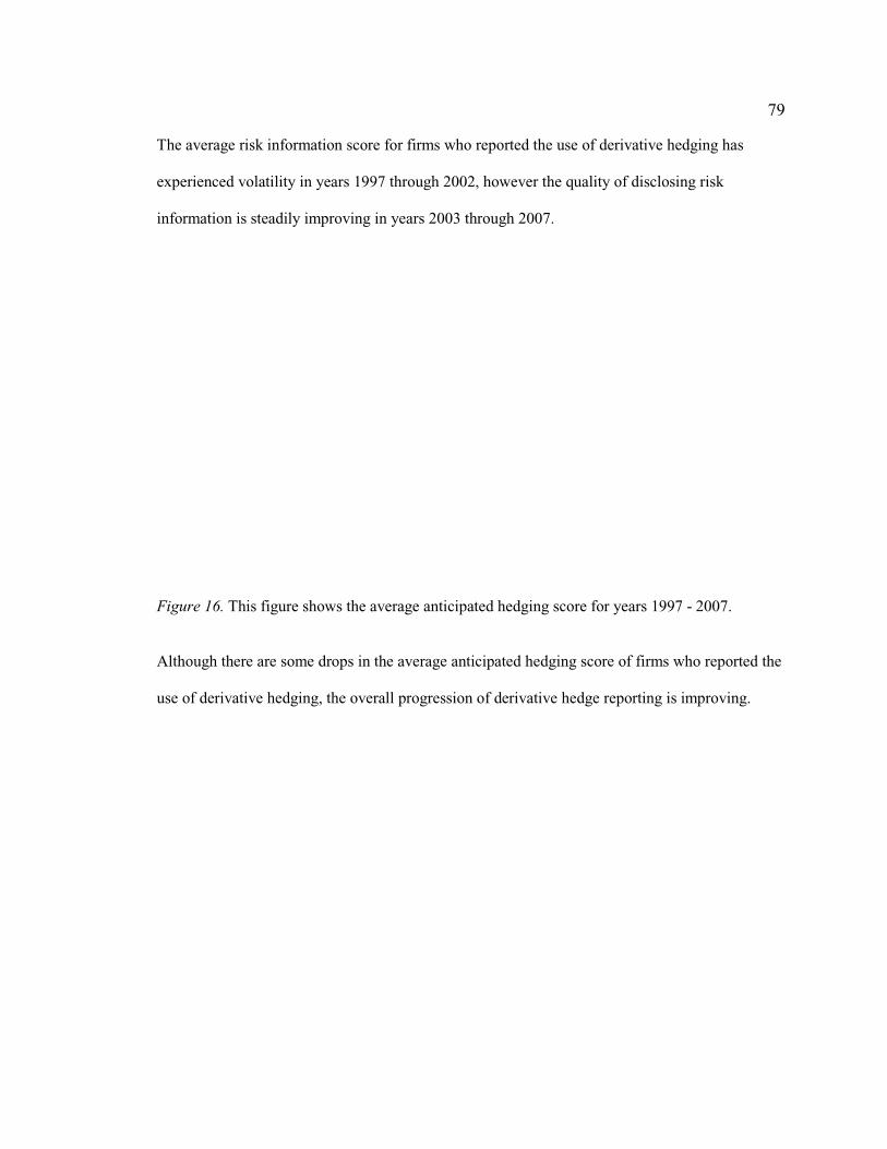
79
The average risk information score for firms who reported the use of derivative hedging has
experienced volatility in years 1997 through 2002, however the quality of disclosing risk
information is steadily improving in years 2003 through 2007.
Figure 16. This figure shows the average anticipated hedging score for years 1997 - 2007.
Although there are some drops in the average anticipated hedging score of firms who reported the
use of derivative hedging, the overall progression of derivative hedge reporting is improving.

80
Figure 17. This figure shows a graphical depiction of the average net fair value scores for years 1997 – 2007.
The average net fair value score for firms who reported the use of derivative hedging in years
1997 – 2007 is steady and is marginally improving.
Figure 18. This figure shows the graphical depiction of the average QDI scores for years 1997 - 2007

81
The average QDI score is a composite of all other transparency categories for the annual reported
years 1998 through 2007. The annual QDI score was below 80% for all firms in the sample for
seven of the eleven years in the data range. The highest annual QDI score of 83% occurred in
2006 with a slight drop (down to 81%) in 2007. However, the overall disclosure quality of
financial reporting is significantly improving. An evaluation of the proportion of QDI scores in
1998 and 2002 is conducted (before and after SFAS No. 133). The QDI scores of firms who
reported the use of derivative hedging are presented in figure 8 and 9.
Figure 19. This figure shows the graphical depiction of the QDI scores for year 1998.
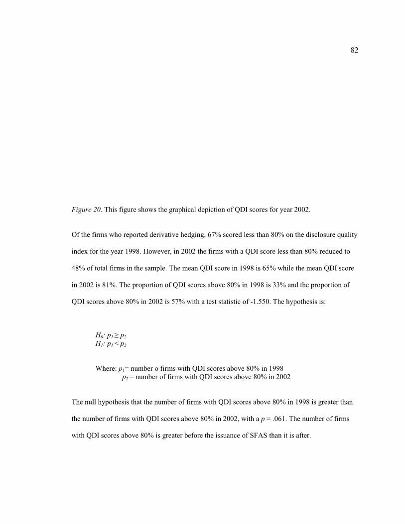
82
Figure 20. This figure shows the graphical depiction of QDI scores for year 2002.
Of the firms who reported derivative hedging, 67% scored less than 80% on the disclosure quality
index for the year 1998. However, in 2002 the firms with a QDI score less than 80% reduced to
48% of total firms in the sample. The mean QDI score in 1998 is 65% while the mean QDI score
in 2002 is 81%. The proportion of QDI scores above 80% in 1998 is 33% and the proportion of
QDI scores above 80% in 2002 is 57% with a test statistic of -1.550. The hypothesis is:
H0: p1 p2
H1: p1 < p2
Where: p1= number o firms with QDI scores above 80% in 1998 p2 = number of firms with QDI scores above 80% in 2002
The null hypothesis that the number of firms with QDI scores above 80% in 1998 is greater than
the number of firms with QDI scores above 80% in 2002, with a p = .061. The number of firms
with QDI scores above 80% is greater before the issuance of SFAS than it is after.

83
Evidence 1998 2002 Size 21 21 n
# of QDI Scores above 80% 7 12 x Proportion 0.33 0.57 p-hat
Hypothesis Testing Hypothesized Difference Zero Pooled p-hat 0.452
Test Statistic -1.550 z At an of Null Hypothesis p-value 0.05 H0: p1 - p2 = 0 0.121 H0: p1 - p2 >= 0 0.061 H0: p1 - p2 <= 0 0.939
Figure 21. This figure shows the summary statistics for the QDI population proportion for years 1998 – 2002. The p-hat is the proportion of individuals having the characteristic when the two samples are lumped together.
Summary
Research question 1 is a comparative investigation of total cash earnings and total net
accruals. Aggregate t tests are conducted to examine the difference in means of total cash
earnings and total net accruals for the periods 1997 through 2007 with a sensitivity test conducted
for all periods 1997 – 2007. The results are statistically significant and indicate the means for
total cash earnings are greater than the means for total net accruals for all years 1997 through
2007. The degree of dispersion around the mean, measured by the standard deviation is greater
for total net accruals than for total cash earnings with the exception of periods 1997, 1998, and
2000. These findings suggest total cash earnings are greater than total net accruals however, total
net accruals are more volatile reflective of dispersion around the mean.
Research question 2 is a correlational investigation of the discretionary component of
total net accruals. The modified Jones model is used to stratify non-discretionary accruals from
total net accruals and the difference is calculated to yield the total discretionary accrual activity.
The analysis includes the use of a multiple regression model that is used to regress the total net
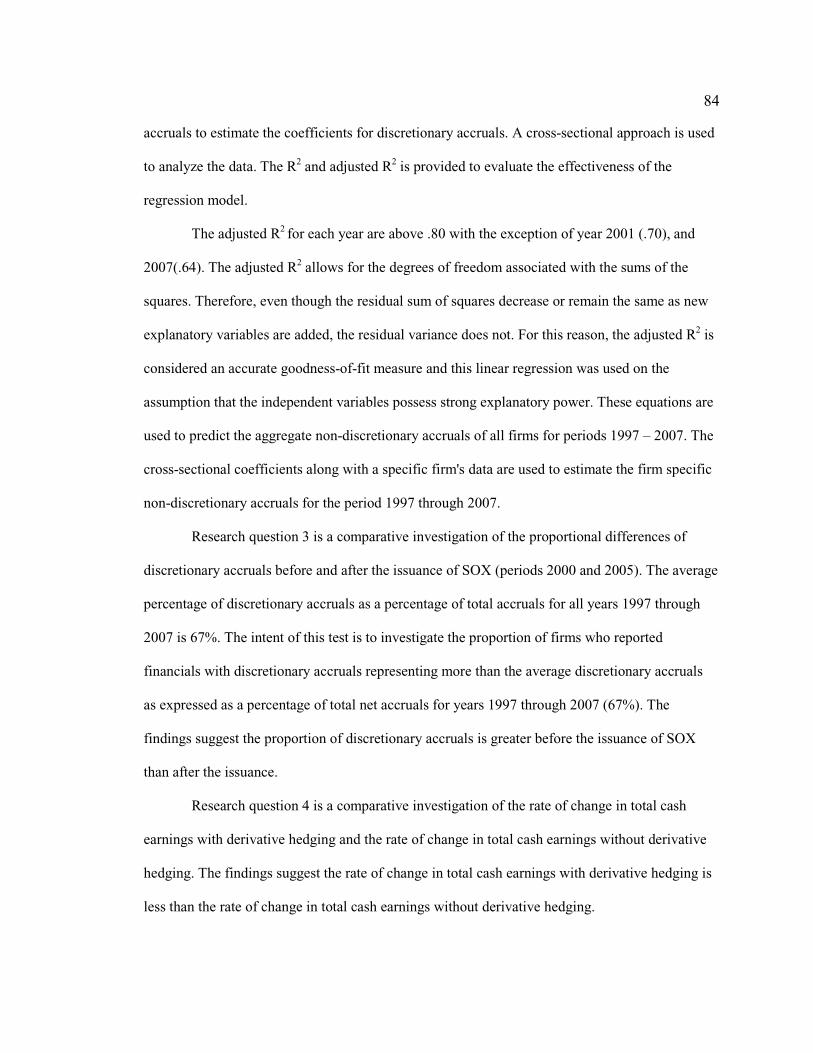
84
accruals to estimate the coefficients for discretionary accruals. A cross-sectional approach is used
to analyze the data. The R2 and adjusted R2 is provided to evaluate the effectiveness of the
regression model.
The adjusted R2 for each year are above .80 with the exception of year 2001 (.70), and
2007(.64). The adjusted R2 allows for the degrees of freedom associated with the sums of the
squares. Therefore, even though the residual sum of squares decrease or remain the same as new
explanatory variables are added, the residual variance does not. For this reason, the adjusted R2 is
considered an accurate goodness-of-fit measure and this linear regression was used on the
assumption that the independent variables possess strong explanatory power. These equations are
used to predict the aggregate non-discretionary accruals of all firms for periods 1997 – 2007. The
cross-sectional coefficients along with a specific firm's data are used to estimate the firm specific
non-discretionary accruals for the period 1997 through 2007.
Research question 3 is a comparative investigation of the proportional differences of
discretionary accruals before and after the issuance of SOX (periods 2000 and 2005). The average
percentage of discretionary accruals as a percentage of total accruals for all years 1997 through
2007 is 67%. The intent of this test is to investigate the proportion of firms who reported
financials with discretionary accruals representing more than the average discretionary accruals
as expressed as a percentage of total net accruals for years 1997 through 2007 (67%). The
findings suggest the proportion of discretionary accruals is greater before the issuance of SOX
than after the issuance.
Research question 4 is a comparative investigation of the rate of change in total cash
earnings with derivative hedging and the rate of change in total cash earnings without derivative
hedging. The findings suggest the rate of change in total cash earnings with derivative hedging is
less than the rate of change in total cash earnings without derivative hedging.
85
Research question 5 is a comparative investigation conducted to investigate the
proportion of the quality of disclosed financial statements of firms who reported the use of
derivative hedges. Each firm in the sample is evaluated in terms of risk, hedging, fair value, and
accounting information provided in annual reports and financial statements. The quality
disclosure index score (QDI) is calculated by assigning a 1 for reporting the information and a 0
if otherwise. Then all scores are summed and divided by the possible score. The findings suggest
the proportion of firms with QDI scores of 80% or above for firms who used derivative hedging
were greater in 1998 than they were in 2002 (greater before the issuance of SFAS No. 133 than
after).
In the next chapter, the interpretation of findings, inferences from study results are
provided, the impacts to positive social change are explained, and recommendations for further
research are introduced.

CHAPTER 5:
SUMMARY, CONCLUSION, AND RECOMMENDATIONS
Earnings management activities through the use of discretionary accruals and derivative
hedging are a central concern because of the financial impact on society as a whole and the
widening financial exposure of mispricing assets (Bartov, Givoly, & Hayn, 2002). The U.S.
Congress and the Financial Accounting Standards Board has introduced regulation with the
efforts to minimize ambiguity in derivative hedging and to enhance transparency in financial
reporting. The Statements of Financial Accounting Standards No. 133, Accounting for Derivative
Instruments and Hedging Activities (SFAS No. 133) was created in 2001 in response to
significant hedging losses involving derivatives (Dubofsky, & Miller, 2003). The intent of SFAS
No. 133 was to control and manage corporate hedging as risk management not earnings
management activities (Barton, 2001). However, based on the events that have lead to the
convergence of financial markets in 2007, it is evident that earnings management activities have
found a place in derivative hedging (Minton, Stulz, & Williamson, 2009). The Sarbanes- Oxley
Act issued in 2002, was created to strengthen corporate accounting controls. Yet, earnings
smoothing through the use of discretionary accruals is increasing in the high technology industry
sector—a sector regarded as income conservative (Uday, Wasley & Waymire, 2004).
Problems Encountered
Only U. S. firms identified as high technology firms by SIC code and possess reported
financial data for years 1998 through 2007 were included in this study. To satisfy this
requirement, two firms were dropped from the sample (firms with ticker codes MXIM and JDSU)
and two firms were randomly drawn from the population defined by SIC code (firms with ticker
codes LSCC and CTXS) to yield 30 companies. This analysis is based on the published financial
87
statements and annual reports of firms in the sample therefore the accuracy of this study is limited
to financial information reported to the Securities and Exchange Commission during years 1997
through 2007.
The economic crisis of 2007-08 that contributed to the meltdown of the of the U.S. sub-
prime housing market had a variety of implications for the economy. The crisis stifled
international business, spiked global oil and food prices, and brought consumer credit to a halt. It
also created a great deal of uncertainty surrounding the reporting and regulation of financial
markets. In this section, the quantitative findings from the tests conducted in this study are
explained. Each individual research question is answered and a final interpretation of research
findings is provided. The overall contribution to positive social change is presented and
recommendations to existing policy will be presented. The final section lays the groundwork for
future research and includes recommendations for future areas of research.
Interpretation of Findings
Research question 1 focused on the differences between total cash earnings and total net
accruals for high technology firms. The question was addressed with an aggregate t test that is
used to evaluate the difference in means of total cash earnings and total net accruals for all years
1997 through 2007. The intent of this test is to identify differences between these two
populations. The null hypothesis that total cash earnings are equal to total net accruals is rejected
for all years 1997 – 2007 and is statistically significant. The sensitivity t test that evaluates total
cash earnings and total net accruals is also statistically significant with a p < .000. The means of
total cash earnings are greater than the means for total net accruals for all years 1997 through
2007. The findings from the aggregate t test of all years ranging from 1997 to 2007 suggest firms

88
are using estimates that are significantly lower than actual cash earnings. The findings are
consistent with the study conducted by Uday, Wasley, and Waymire in 2004.
The firms in the sample represent the high technology industry segment. The high
technology industry segment has been described as an income conservative practicing
environment (Lobo, & Zhou, 2006). High technology firms face greater risks of shareholder
litigation than other industries (Lobo, Zhou, 2006). High tech industry companies are also
affected to a greater degree by conservative accounting standards on research and development
costs (Uday, Wasley, & Waymire, 2004). The means of total cash earnings are greater than the
means of total accruals for this industry segment; this finding suggests that risk adverse managers
are likely to be more conservative in their financial reporting.
Research question 2 focused on the discretionary accruals calculated by referencing the
modified Jones model to breakout discretionary accruals from non-discretionary accruals. The
estimated regression equations are used to determine the discretionary component of total net
accruals. An evaluation of discretionary accruals activity is conducted.
Research question 3 focused on the proportional differences between discretionary
accruals in 2000 and 2005. The number firms with discretionary accruals representing more than
67% of total net accruals in 2000 is greater than the number of firms with discretionary accruals
representing more than 67% of total net accruals in 2005 (after SOX) (p = .007). In 2000,
discretionary accruals represented 75% of total net accruals and in 2005; discretionary accruals
represented 66% of total net accruals (just 1% less than the average for all years 1997 through
2007). Although the use of discretionary accruals appears to be shrinking in the high technology
industry segment, the discretionary percentage remains high.
Research question 4 focused on the variances in the rate of change in total cash earnings
with derivative hedging and the variances in the rate of change in total cash earnings without
89
derivative hedging. The findings suggest the rate of change in total cash earnings of firms who
use derivative hedging (M = 232.54, SD = 1,109) is less volatile than the rate of change in total
cash earnings of firms who do not use derivative hedging (M = 3,701.91, SD = 8,017). Derivative
hedging therefore minimizes earnings volatility for firms in the high technology industry
segment.
Research question 5 focused on the quality of disclosed financial statements particularly
with regard to derivative hedging. Firms who reported the use of derivative hedging were
evaluated with the use of a quality disclosed index (QDI) to reflect the transparency of financial
reporting in the area of risk, accounting, hedging, and fair value. In the quality disclosure
analysis, 67% of the firms who reported the use of derivative hedging scored less than .80 on the
QDI in 1998. In 2002, 48% of firms who reported the use of derivative hedging scored less than
.80 on the QDI. These findings suggest a 20% increase in the quality of financial transparency
reporting between year 1998 and 2002. However, 55% of firms who reported the use of
derivative hedging in 2007 scored less than .80 on the QDI. A population proportion test was
conducted to test the proportion of quality disclosure reporting between 1998 and 2002. The
descriptive statistics suggest disclosure quality of high technology firms is increasing. However,
the null hypothesis that the number of firms in 1998 with QDI scores above 80% is greater than
the proportion of the firms with QDI scores above 80% in 2002 cannot be rejected (p = .06). This
suggests the quality of disclosure in derivative reporting in 1998 is superior to the quality of
disclosure in derivative reporting in 2002. These findings suggest the QDI scores of firms were
higher before SFAS No. 133 than after the issuance of SFAS No. 133.

90
The QDI scores dropped from .70 in 1997 to .65, in 1998. The largest drop in quality disclosure
scores of firms who reported the use of derivative hedging between 1997 and 1998 is in the risk
information (9.5% decrease) and net fair value information (6.8% decrease) categories. These
findings are consistent with FASB’s response to the significant hedging losses involving
derivatives and the issuance of SFAS No.133. The intent of SFAS No. 133 was to control and
manage corporate hedging as risk management (Barton, 2001).
Conclusions and Implications for Social Change
The accounting treatment of operational activities has a definite impact on reported
earnings. It has been argued firms in the high technology industry segment exercise income
conservatism (Kwon, Yin, & Han, 2006). Total accrual usage has increased and the discretionary
component of accruals has slightly decreased. The proportion of discretionary accruals in 2000 is
greater than the proportion of discretionary accruals in 2005, but the proportion of discretionary
accruals in 2005 is just 1% less than the average discretionary proportion for all years 1997
through 2007. This suggests that management choices (discretionary accruals) represent a
significant portion of financial reporting. It is evident SOX implemented in 2002 has minimized
earnings smoothing through the use of discretionary accruals in the high technology industry
segment.
In addition, the use of derivative hedging is increasing; over 70% of the firms in the
sample reported the use of derivative hedging during the period 1997 through 2007. Derivative
hedging allows firms to establish a leveraged position with minimal margin requirements
(sometimes no collateral required) resulting in an increase in price exposure (Financial
Economists Roundtable. 1994). They are off-balance sheet activities that are not reported with the
same clarity and detail as other securities, loans, or other assets or liabilities (Guay, 1999).

91
The quality disclosure of financial reporting was investigated to examine the
transparency of financial reporting for derivative hedging. The findings suggest the quality of
financial reporting is increasing. The QDI scores of firms were higher before SFAS No. 133 than
they were after the issuance of SFAS No. 133. However, 55% of firms who reported the use of
derivative hedging in 2007 scored less than .80 (out of 1.0) on the QDI. For the aggregate years
1997 through 2007, 51% of firms scored less than .80 on the QDI: hedges of anticipated
transactions category. In addition, 58% of firms scored less than .80 on the QDI: net fair value
category for the aggregate years 1997 through 2007. These findings suggest that 51% of firms in
the high technology industry segment who used derivative hedging during the period 1997
through 2007, did not fully report activities that exposed the firm to market and credit risk.
Derivative hedging does have an impact on a firm’s ability to report stable earnings in the
high tech industry segment. When a firm uses derivative hedging, the variance in the annual rate
of change in total cash earnings is reduced suggesting derivative hedging minimizes real earnings
volatility (Barton, 2001). These findings support Barton’s conclusion that derivative hedging
provides significant value in risk management.
It is clear that earning smoothing activities represent a large portion of reported earnings
in the high technology industry segment. Mixed results follow regulations such as SOX and
FASB 133 with regard to the use of discretionary accruals and derivative hedging. The increase in
earnings management defined by discretionary accruals is alarming considering the lack of
transparency in financial reporting.
Challenges to Neo-Classical Economic Theory
Under the Efficient Market Theory, a perfectly competitive market is a well-functioning
market, where the prices of capital assets (securities) reflect predictions based on all relevant and
92
available information (Anderson, Caldwell, & Needles, 1994). This concept holds that securities
prices established in financial markets, fully reflect all the available and relevant information to
investors. The assumption is that security prices follow a random walk (Basu, 1977). The premise
is that if all relevant information is reflected in the current market price, then only meaningless
noise is left to explain price movements. However, these rules can not apply to a financial
instrument that presents no market reference for pricing or lies outside the reporting requirements
of other securities.
Another axiom of efficient market theory is that investors cannot systematically beat the
performance of the market because all relevant market information is used to determine the price
and any future changes in price are sporadic (Laffont, & Maskin, 1990). Any price that does
reflect the perfectly informed fundamentals creates the possibility of arbitrage trading that will
drive the price back to the level thus reflecting informed fundamentals resembling a price
correction (Brenner, 1979). However, from the findings of this study and from the examples
illustrated in the collapse of Enron in 2001, and the onslaught of government financial bail outs of
2009; it is evident that financial markets are imperfect as a result of information asymmetry. It is
apparent that a significant level of disparity exists between actual characteristics of financial
markets and the assumptions of neo-classical economic theory.
Under the Capital Asset Pricing Model (CAPM created by William Sharpe and John
Lintner), market behavior can be explained by pricing risk in financial markets (Jagannathan, &
Wang, 1996). The premise of the CAPM is that securities are efficiently priced by financial
markets according to their relative risk (beta) compared to the inherent risk in the market as a
whole. Under this model, risk is determined by the degree of volatility (Sharpe, 1964). The
greater the degree of variation measured by beta, the lower the price of the security. This premise
suggests the market rewards lower risk securities with a higher price and higher risk securities
93
with a greater return on investment (Harris, & F., 2001). However, this efficient-risk-reward
relationship applies only to the direct ownership of the security. When a firm uses derivatives for
hedging (or speculating) they are diverting the risk to others. This risk shifting stimulates risk
exposure to outside counterparties (Jagannathan, & Wang, 1996). For example, Enron’s collapse
drove natural gas prices down across the U.S. after its counterparties lost their positions which
required them to replace their short-hedge position on the NYMEX or selling its inventory
(Benston, & Hartgraves, 2002). It is apparent that hedging risk can result in a rippling effect to
individuals with no direct exposure to the defaulting party. Therefore, current markets conditions
cannot address all the aspects of risk hedging. Due to these market imperfections formulated by
the lack of transparency in derivative reporting and the intent of risk diverting; the establishment
of market equilibrium and the creation of efficient markets cannot be achieved (Niranjan, Quan,
& Meenakshi, 2007). These market imperfections, short-comings and other failures result in
externalities that all individuals in the economy must bear.
Contributions to Positive Social Change
This study provides evidence to managers, investors, and legislators that earning
management activities represent a significant portion of total accruals. It has been shown that the
accounting treatment of operational activities has an impact on the ability to stabilize reported
earnings. The evidence also indicates regulation such as SOX and SFAS No. 133 has not
eliminated earning management activities through the use of discretionary accruals or derivative
hedging in the high technology industry segment.
This analysis contributes to positive social change by highlighting the significance of
these findings and by introducing externalities that have surfaced as a result of the lack of
transparency in financial reporting. It is essential that government regulation play a leading role
in setting reporting standards. Free and competitive markets cannot exist with these types of
94
financial instruments. The rippling effects of these instruments extend beyond neo-classical
economics of market discipline. In some cases, market competition actually drives participants to
hold less and less capital relative to their risk exposure (Abdel-khalik, 2006). The linkages of
these externalities are clearly demonstrated by the collapse of the Enron Corporation in 2001
when the effects of the bankruptcy spread beyond stock and bond holders, employees and
immediate creditors (Benston, & Hartgraves, 2002). To enhance financial markets and contribute
to positive social change, I make the following suggestions for regulation modification:
1. Require disclosure of all derivative activities on balance sheet reports and
mandate the reporting of prices and other critical market information. Improve
market transparency by increasing the quantity and quality of available
information to investors.
2. Supervise and examine financial institutions and report on their condition.
3. Collect and help disseminate data. Government regulators should collect accurate
and unbiased information (enforceable by law) with a consistent methodology to
provide price data over a long periods of time, and should distribute the
information in a timely, fair and affordable manner.
Recommendations for Future Study
In the fall of 2008, a severe market correction occurred in the financial sector that
stemmed in large part to the real estate market. As Lehman Brothers filed for bankruptcy, Bank of
America acquired Merrill Lynch and companies ranging from Washington Mutual to AIG were
tendering on the edge of bankruptcy (Hong, Keejae & Kyonghee, 2009). In response to this
financial crisis, Congress passed the Emergency Stabilization Act of 2008. This Act provided the
authority for the Federal Government to purchase and ensure certain types of troubled assets for

95
the purposes of providing stability to and preventing disruption in the economy and financial
system as well as protecting taxpayers.
Most companies in the economy will experience a rippling effect of the market
adjustment (Minton, Stulz, & Williamson, 2009). It is conceivable that the high tech sector may
be partially sheltered from the brunt of the financial crisis as firms try to spend more on
technology in order to reduce the operational costs. More in depth research in the area of earnings
smoothing prior to and after the financial crisis of 2008 is needed. Areas for future research
include derivative hedging in the financial markets, earnings smoothing and management
discretion in the financial sector, and financial impacts of the Emergency Stabilization Act of
2008.
Summary
It is time to reconsider the assumptions of the feasibility of a truly capital driven financial
market. The assumptions embedded in the academic areas of finance must be re-evaluated to
include human behavioral traits. From this study, it is evident the assumptions that participants
act rationally and that the market is efficient is no longer valid. Under the Efficient Market
Theory, a perfectly competitive market is a well-functioning market, where the prices of capital
assets (securities) reflect predictions based on all relevant and available information (Anderson,
Caldwell, & Needles, 1994); however, if all relevant information is not available (and in most
cases it is not available) the assumptions of the Efficient Market Theory no longer hold. In
addition, the rules of efficient markets can not apply to financial instruments that present no
market reference for pricing or for financial instruments that are unreported and thus reside
outside the reporting requirements of other securities.

96
Assumptions that are inherent in the Capital Asset Pricing Model (CAPM) must also be
re-examined as a result of the findings of this study. The premise of the CAPM is that securities
are efficiently priced by financial markets according to their relative risk (beta) compared to the
risk of the market as a whole. Under this model, risk is determined by the degree of volatility
(Sharpe, 1964). The greater the degree of variation measured by beta, the lower the price of the
security. This premise suggests the market rewards lower risk securities with a higher price and
higher risk securities with a greater return on investment (Harris, & F., 2001). However, this
efficient-risk-reward relationship applies only to the direct ownership of the security and excludes
the utilization of derivative hedges. When a firm uses derivatives for hedging (or speculating),
they are diverting the risk to others. This risk shifting stimulates risk exposure to outside
counterparties (Jagannathan, & Wang, 1996). It is apparent that hedging risk can result in a
rippling effect to individuals with no direct exposure to the defaulting party. The current markets
conditions cannot address all the aspects of risk hedging. Due to these market imperfections
formulated by the lack of transparency in derivative reporting and the intent of risk diverting, the
establishment of market equilibrium and the creation of efficient markets cannot be achieved.
These market imperfections, short-comings, and other failures result in externalities that all
individuals in the economy will bear.

REFERENCES
Abdel-khalik, A. R. (2006). An empirical analysis of CEO risk Aversion and the propensity to smooth earnings volatility [Monograph].
AERA (2006). Standards for reporting on empirical social science research in AERA publications. Educational Researcher, 35, 33-40.
Ahmed, K. & Courtis, J.K. (1999). Associations between corporate characteristics and disclosure levels in annual reports: A meta-analysis. British Accounting Review. 31, 35-61.
Allayannis, G.S., & Ofek, E. (1997) Exchange rate exposure, hedging, and the use of foreign currency derivatives [Monograph].
Allayannis, G., Rountree, B., & Weston, J.P. (2008). Do investors value smooth performance? Journal of Financial Economics, 90(3), 237-251.
Anderson, H., Caldwell, J., & Needles, B. Jr. (1994). Financial & Managerial Accounting (3rd
ed.). Boston: Houghton Mifflin Co.
Aczel, A. D., & Sounderpandian, J. (2002). Complete Business Statistics (5th ed.). New York, McGraw-Hill Publishing Co.
Aono, J.Y., & Guan, L. (2007). The impact of the Sarbanes-Oxley Act on cosmetic earnings management. Research in Accounting Regulations, 20.
Ball, R., & Brown, P. (1968). An empirical evaluation of accounting income numbers. Journal of Accounting Research, 8, 159-178.
Barnes, R. (2003). Earnings volatility and market valuation: An empirical investigation. London Business School, Working Paper.
Barton, J. (2001). Does the use of financial derivatives affect earnings management decisions? The Accounting Review, 76 (1), 1-26.
Barton, J., & Simko, P. J. (2002). The balance sheet as an earnings management constraint. The Accounting Review, 77 (Supplement), 1-27.
Bartov, E., Givoly, D., & Hayn, C. (2002). The rewards to meeting or beating earnings expectations. Journal of Accounting and Economics, 33, 173-204.
Bartov, E., & Gul, F. (2001) Discretionary-accruals models and audit qualifications. Journal of Accounting and Economics, 33,(3), 375-400
Basu, S. (1977) Investment performance of common stocks in relation to their price-earnings ratios: A test of the Efficient Market Hypothesis. Journal of Finance, 32, (3), 663-682.
98
Beattie, V., Brown, S., Ewers, D., John, B., Manson, S., Thomas, D., & Turner, M. (1994). Extraordinary items and income smoothing: A positive accounting approach. Journal of Business Finance & Accounting, 21(6), 791–811.
Beatty, A. L., Ke, B., & Petroni, K. R. (2002). Earnings management to avoid earnings declines across publicly and privately held banks. The Accounting Review, 77(3), 547-570.
Benston, G.J., & Hartgraves, A.L. (2002) Enron: what happened and what we can learn from it. Journal of Accounting and Public Policy, 21(2), 105-127.
Blankey, A. & R. Schroeder. (2000). Accounting for derivatives under SFAS No. 133. The Mid-Atlantic Journal of Business. 36(1), 17-35.
Bodnar, G., Gregory, S., Hayt, S., Richard, C. M. (1998). Wharton survey of financial risk management by US non-financial firms. Financial Management, 27(4), 70-91.
Bodnar, Gordon M. & Gebhardt, Günther, (1998) Derivatives usage in risk management by US and German non-financial firms: A comparative survey. NBER Working Paper No. W6705.
Bowen, R. M., Rajgopal, S., Venkatchalam, M, (2004). Accounting discretion, corporate governance and firm performance. Working paper, University of Washington and Duke University.
Bowman, Robert G. , Navissi, Farshid, & Burgess, Richard C. (1991) Regulatory threats and political vulnerability. Journal of Financial Research.
Boynton, Charles, E., Paul S. Dobbins, Paul, S., & Plesko, George, A. (1992). Earnings management and the corporate alternative minimum tax. Journal of Accounting Research, 30, 131-153.
Brown, L. D., and Caylor, M. L. (2005). A temporal analysis of quarterly earnings thresholds: Propensities and valuation consequences. The Accounting Review,80, 423-440.
Brown, G., Crabb, P., & Haushalter, D. (2003). Are firms successful at selective hedging? Pennsylvania State University, working paper.
Brenner, M. (1979). The sensitivity of the Efficient Market Hypothesis to alternative specifications of the market model. Journal of Finance, 34(4), 915-929.
Bruns, W. J., & Merchant, K. A. (1990). The dangerous morality of managing earnings. Management Accounting, 72(2), 22-26.
Burgstahler, D.C., & Dichev, I. D (1997). Earnings management to avoid earnings decreases and losses. Journal of Accounting and Economics, 24(1), 99-126.
Burgstahler, D.C., & Dichev, I. D. (1997). Earnings, adaptation and equity value. The Accounting Review, (April), 187-215.
99
Carter, M. E., Lynch, L. J., & Zechman, S. (2006). The relation between executive compensation and earnings management: Changes in the post-Sarbanes-Oxley era. University of Pennsylvania, working paper.
Chaney, P.K., Jeter, D.C., & Lewis, C.M. (1998). The use of accruals in income smoothing: a permanent earnings hypothesis. Advances in Quantitative Analysis of Finance and Accounting, 6:103-135.
Chez, C., & Fuentes, F.P. (2004). Long-run abnormal returns and income smoothing in the Spainish stock market. European Accounting Review, 13(1), 105-130.
Chung-Hua Shen, Chung H., & Chih, H. (2005). Investor protection, prospect theory, and earnings management: An international comparison of the banking industry. Journal of Banking & Finance, 29(10), 2675-2697.
Cohen, D. A., Dey, A, & Lys, T. (2004). Trends in earnings management and informativeness of earnings announcements in the pre- and post-Sarbanes-Oxley periods. Northwestern University working paper.
Cohen, J. (1977). Statistical Power Analysis for Behavioral Sciences (revised ed.). New York: Academic Press.
Cohen, J. (1990). Things I have learned (so far). American Psychologist, 45, 1304-1312.
Collingwood, H. (2001). The earnings game: Everyone plays, nobody wins. Harvard Business Review, 79(6), 65-77.
Collins, D. W., & Hribar, P. (2000). Errors in estimating accruals: Implications for empirical research. Journal for Accounting Research.
Collins, D.W., & Hribar, P. (2002). Errors in Estimating Accruals: Implications for Empirical Research. Journal of Accounting Research, 40(1), 105-134.
Coppens, L., & Peek, E. (2005). An analysis of earnings management by european private firms. Journal of International Accounting, Auditing and Taxation, 14, 1-17.
Crutchley, C.E., Jensen, M.R., & Marshall, B.B. (2007). Climate for scandal: Corporate environments that contribute to accounting fraud. The Financial Review 42(1), 53–73.
Da Silva Rosa, R., Sheung, A., & Terry, W. (2003). Market reaction to share buybacks and special dividends under a tax imputation system.
Damodaran, A. (2004). Investment fables. New York, John Wiley and Sons.
Das, S., & Shroff, P. K. (2002). Fourth quarter reversals in earnings changes and earnings management. University of Illionois, Working paper.

100
Dechow, P.M., Sloan R.G., & Sweeney, A.P. (1995). Detecting earnings management. The Accounting Review,70(2),193-225.
Dechow, P. M., & Skinner, D. J. (2000). Earnings management: Reconciling the views of accounting academics, practitioners, and regulators. Accounting Horizons, 14(2), 235-250.
Dechow, P. M., Richardson, S., & Tuna, I. (2003). Why are earnings kinky? An examination of the earnings management explanation. Review of Accounting Studies, 8, 355-384.
DeGeorge, F., Patel, J., & Zeckhauser, R.(1999). Earnings management to exceed thresholds. Journal of Business Research, 72(1), 1-33.
Dubofsky, D. A., & Miller, T. W. (2003). Derivatives : Valuation and risk management. London, Oxford University Press.
DuCharme L., Malatesta, P., & Sefcik, S. (2004). Earnings management, stock issues, and shareholder lawsuits. Journal of Financial Economics 71, 27-49.
Dunham, P. J. (1988). Research methods in psychology. New York: Harper and Row.
Epps, R. W., & Guthrie, C. P. (2007). Sarbanes-Oxley 404 Material Weaknesses and Discretionary Accruals(October 1, 2007). Accounting Forum.
Emery, Douglas, R., & Finnerty, John, D. (1997). Corporate financial management. Upper Saddle River, New Jersey.
Financial Accounting Standards Board. (1991). Statement of Financial Accounting Standards No 107 Disclosures about Fair Value of Financial Instruments. Financial Accounting Standards Board of the Financial Accounting Foundation.
Financial Accounting Standards Board. (1994). Statement of Financial Accounting Standards No 119: Disclosure about Derivative Financial Instruments and Fair Value of Financial Instruments. Financial Accounting Standards Board of the Financial Accounting Foundation.
Financial Accounting Standards Board. (1998). Statement of Financial Accounting Standards No 133 Accounting for Derivative Instruments and Hedging Activities. Financial Accounting Standards Board of the Financial Accounting Foundation.
Financial Economists Roundtable (1994) Derivatives markets and financial risk: 1995 the structure of the NASDAQ stock market.
GAO. Report to the Congress. Financial audit resolution trust RTC’s financial statements.Retrieved August 2007, from www.gao.gov/archive/1996/ai96123.pdf
Garza-Gómez, X.; Okumura, M., and Kunimura, M. (2000). Discretionary Accrual Models and the Accounting Process. Kobe Economic & Business Review, 45, 103-135.
101
Gaver, K.M., Austin, J.R., & Gaver, J.J. (1995) Additional evidence on bonus plans and income management. Journal of Accounting and Economics, 19, (1)3-28.
Geczy, C., Minton, B. A., & Schrand, C. M. (2005). Taking a view: Corporate speculation, governance and compensation. University of Pennsylvania, Working paper.
Gerry, Grant H., (2003). Maynard manufacturing: An analysis of GAAP-based and operational earnings management techniques, Strategic Finance, 85(1).
Glaum, M., Lichtblau K., & J. Lindemann, J. (2004). The extent of earnings management in the US and Germany. Journal of International Accounting Research, 3, 45–77.
Gore, P., Pope, P. F., & Singh, A. K. (2002). Earnings management and the distribution of earnings relative to targets: U.K. evidence. Working paper, British Accounting Association annual conference.
Graham, J., Harvey, C., and Rajgopal, S. (2005). The economic implications of corporate financial reporting. Journal of Accounting and Economics, 40(1-3), 3-73.
Guay, W.R. (1999). The impact of derivatives on firm risk: An empirical examination of new derivative users. Journal of Accounting and Economics, 26, (1-3), 319-351.doi:10.1016/S0165-4101.98.00032-9
Guay, W., & Kothari, S.P. (2003). How much do firms hedge with derivatives?, Journal of Financial Economics, 70, 423-461.
Guay, W., Kothari, S. P., & Watts, Ross, L. (1996) A market-based evaluation of discretionary accrual models. Journal of Accounting Research, 34, 83-105.
Hagart, Gordon.,& Knoepfelon, Ivo. (2006) Conference Report: ESG value drivers. Company-Investor Interface.
Healy, P.M. (1985). The effect of bonus schemes on accounting decisions. Journal of Accounting and Economics, 7(1-3), 85-107.
Harris, R. S. and F. C. Marston (2001). The market risk premium: Expectational estimates using analysts' forecasts. Journal of Applied Finance 11(1), 6-11.
Healy, P.M. (1985). The effect of bonus schemes on accounting decisions. Journal of Accounting and Economics, 7(1-3): 85-107.
Heiman, G.A. (1995). Research methods in psychology. Boston, MA: Houghton Mifflin
Heflin, F., K.W. Shaw and J.J. Wild (2001). Disclosure quality and market liquidity. Working Paper. Purdue University.
Henock, Louis, (2004) Earnings management and the market performance of acquiring firms. Journal of Financial Economics, 74(1), 121-148.

102
Hentschel, L., & Kothari, S. (1999). Are corporations reducing or taking risks with derivatives? Working paper, University of Rochester, Rochester, NY.
Hiemstra, C., & Jones, J.D., (1994) Testing for linear and nonlinear Granger Causality in the stock price- volume relation. The Journal of Finance, 49(5),1639-1664.
Hong, D. S., Keejae & Kyonghee, K. (2009), Cash flow volatility, income smoothing and CEO cash compensation.
Hribar, P., & Collins, D. (2002). Errors in estimating accruals: Implications for empirical research. Journal of Accounting Research, 40(1), 105-134.
Huang, P., Ryan, H.E., & Wiggins, R.A. (2007) The influence of firm and CEO specific characteristics on the use of nonlinear derivative instruments. Journal of Financial Research, 30(3), 415 – 436. doi: 10.1111/j.1475.6803.2007.00221
Huddart, Steven J. & Louis, Henock. (2008). Insider selling, earnings management, and the 1990s stock market bubble.
Hunt, A., Moyer, S.E., & Shevlin, T. (1997). Earnings volatility, earnings management and equity value. Working paper, University of Washington.
Imhoff, E.A. Jr. (1992). The relation between perceived accounting quality and economic characteristics of the firm. Journal of Accounting and Public Policy.11, 97-118.
International Monetary Fund Country Report No 05/216.
Jagannathan, R., & Wang, Z. (1996) The conditional CAPM and the cross-section of expected returns. Journal of Finance, 51(1), 3-53.
Jones, J. J. (1991). Earnings management during import relief investigations. Journal of Accounting Research, 29, 193-228.
Kawaller, I.G. (2004). Perspectives: What analysts need to know about accounting for derivatives. Financial Analysts Journal, 60(2), 24-30.
Kirschenheiter, M., & Melumad, N. D. (2002) Can big bath and earnings smoothing co-exist as equilbrium financial reporting strategies? Journal of Accounting Research, 40(3) 761-796.
Kothari, S.P., Leone, A.J., & Wasley, C.E. (2005). Performance matched discretionary accrual measures. Journal of Accounting & Economics, 39(1), 163-197.
Kothari, S.P., & R. L., Watts. (1996). A market-based evaluation of discretionary accrual models, Journal of Accounting Research, 34, 19-36.

103
Kwon, S., Yin, Q., & Han, J. (2006). The effect of differential accounting conservatism on the over-valuation of high-tech firms relative to low-tech firms. Review of Quantitative Finance and Accounting, 27(2), 143-173.
Laffont, J., & Maskin, E. (1990) The Efficient Market Hypothesis and insider trading on the stock market. Journal of Political Economy, 98(1), 70-93.
Lapointe-Antunes, Pascale; Cormier D., Magnan, M.; & Gray-Angers, Sophie. (2006), On the relationship between voluntary disclosure, earnings smoothing and the value-relevance of earnings: The case of Switzerland. European Accounting Review, 15(4), 465-505.
Leander, E. (1997). Derivatives secrets. Treasury and Risk Management, 7(5), 20-25.
Leuz, C.,Nanda, D., & Wysocki, P. (2003) Earnings management and institutional factors: An international comparison. Journal of Financial Economics, 69(3), 505-527.
Liu, C. (2004). The Sarbanes-Oxley Act and mitigation of earnings management. University of Hawaii, working paper.
Liu, M. H., & Yao, T. (2003). The consensus-beating game. University of Arizona, working paper.
Lobo, G. J., & Zhou, J. (2006). Did conservatism in financial reporting increase after the Sarbanes-Oxley Act? Initial evidence. Accounting Horizon, 20(1), 57-73.
Malone, D., Fries, C., & T. Jones. (1993). An empirical investigation of the extent of corporate financial disclosure in the oil and gas industry. Journal of Accounting, Auditing, and Finance. 8(3), 249-273.
Mann, H. B., & Whitney, D. R. (1947). On a test of whether one of two random variables is stochastically larger than the other. Annals of Mathematical Statistics, 18, 50–60.
McKee, T. E. (2005). Earnings management: An executive perspective. Mason, OH., Thomson.
Melumad, N., Weyns, G., & Ziv, A. (1999). Comparing alternative hedge accounting standards: Shareholders perspective. Review of Accounting Studies, 5, 265-292.
Mian, S. (1996). Evidence on corporate hedging policy. Journal of Financial and Quantitative Analysis, 31, 419-439.
Mills, L., & Newberry, K. (2001). The influence of tax and nontax costs on book-tax reporting differences: Public and private firms. Journal of the American Taxation Association, 23(1), 1-19.
Minton, B.A., Stulz, R., & Williamson, R. (2009) How much do banks use credit derivatives to hedge loans? Journal of Financial Services Research, 35(1), 1-31. doi: 10.1007/s10693.008.0046.3
104
Myers, L.A., & Skinner, D.J. (1999). Earnings momentum and earnings management. Working paper, University of Michigan.
Myers, James, N., Myers, Linda, A., & Omer, Thomas, C. (2003) Exploring the term of the auditor-client relationship and the quality of earnings: A case for mandatory auditor rotation? The Accounting Review, 78, (3), 779-799.
Naor, N. (2006). Reporting on financial derivatives: A law and economics perspective. European Journal of Law and Economics, 21(3), 285-314.
Niranjan, C., Quan , V., & Meenakshi, R. ( 2007) Portfolio flows to emerging capital markets: Do Ccrporate transparency and public governance matter? Business and Society Review,112(2), 227-249.
Nissim, D., & Penman, H. (2003). The association between changes in interest rates, earnings and equity values. Contemporary Accounting Research, 20(4), 775-804.
Peasnell, K.V., & Pope, P.F. (2000) Detecting earnings management using cross-sectional abnormal accrual models. Accounting and Business Research Retrieved July 1, 2008, from http://citeseerx.ist.psu.edu
Pincus, M., & Rajgopal, S. (2002). The interaction of accrual management and hedging: Evidence from oil and gas firms. The Accounting Review, 71,127-160.
Riahi-Belkaouhi. A. (2001). Level of multinationality, growth opportunities, and size as determinants of analysts ratings of corporate disclosures. American Business Review. June,115-120.
Ribstein, L. E.(2002). Market vs. regulatory responses to corporate fraud: A critique of the Sarbanes-Oxley Act of 2002. Journal of Corporation Law, 28(1).
Romano, R. (2005) The Sarbanes-Oxley Act and the Making of Quack Corporate Governance.[Monograph].
Roosenboom, P., Goot, T., & Mertens, G.(2003). Earnings management and initial public offerings: Evidence from the Netherlands. International Journal of Accounting. 38(3), 243-266.
Seaver, W.B. (1973). Effects of naturally induced teacher expectancies. Journal of Personality and Social Psychology, 28, 333-342.
Sengupta, P. (1998). Corporate disclosure quality and the cost of debt. The Accounting Review.73(4) 459-474.
Sharpe, W. F. (1964). Capital asset prices: A theory of market equilibrium under conditions of risk. Journal of Finance, 19(3), 425-442.
105
Shaw, K.W. (2002). Corporate disclosure quality, earnings smoothing, and earnings’ timeliness. Journal of Business Research. 1-8.
Sheedy, E. (1997). Marketing derivatives: a question of trust. International Journal of Bank Marketing, 15(1), 22-31.
Singh, A. (2004). The effect of SFAS 133 on the corporate use of derivatives, volatility, and earnings management. University of Pennsylvania, Working paper.
Shivakumar, L. (1996). Essays Related to Equity Offerings and Earnings Management. Dissertation. Vanderbilt University.
Skinner, D. J., & Sloan, R. G. (2002). Earnings surprises, growth expectations, and stock returns: Don’t let an earnings torpedo sink your portfolio. Review of Accounting Studies, (7), 289-312.
Sloan, R. G. (1996). Do stock prices fully reflect information in accruals and cash flows about future earnings? The Accounting Review, 71(3), 289-315.
Subramanyam, K.R. (1996). The pricing of discretionary accruals. Journal of Accounting and Economics, 22, (1-3), 249-281.
Tarpley, R. L. (2003). How are earnings managed? Examples from auditors. Accounting Horizon, 17, 17-35.
Trombley, M.A. (2003). Accounting for Derivatives and Hedging. McGraw-Hill/Irwin. International Edition.
Tucker, J.W., & Zarowin, P.A. (2006). Does income smoothing improve earnings informativeness? The Accounting Review, 81(1), 251-270.
Tully, S. (2007). Big profits = danger ahead!, Forbes, March 19, 2007, p 196.
Uday, C., Wasley C.E., & Waymire,G.B. (2004). Income conservatism in the U.S. technology sector [Monograph].
Wallison, P.J., & Hassett, K. A. (2004). A trouble requirement: Why should the FASB require the expensing of options if it has no idea how it should be done. Regulation Magazine, 27(1),52-58.
Watts, R. (2003). Conservatism in accounting part I: Explanations and implications. Accounting Horizons, 17(3), 207-221.
Wolf, F.M. (1986). Meta-analysis: Quantitative Methods for Research Synthesis. Beverly Hills, CA: Sage.
Xiong, Yan NMI, & Stammerjohan,William W.(2004) The Economic Profitability of IPO Underperformance. Retrieved May 12, 2008, from http://ssrn.com/abstract=591686

106
Xie, Biao, Davidson, Wallace III, & DaDalt, Peter J. (2003). Earnings management and corporate governance: The role of the board and the audit committee. Journal of Corporate Finance, 9(3), 295-316.
Young, S. (1999). Systematic measurement error in the estimation of discretionary accruals: and evaluation of alternative modeling procedures. Journal of Business Finance & Accounting, 26(7-8): 833-862.
Zhang, Wei NMI2, Zhou, Jian & Lobo, Gerald J., (1996) The Impact of Corporate Governance on Discretionary Accrual Changes Around the Sarbanes-Oxley Act.
Zhou, J. (2007) Financial Reporting After the Sarbanes-Oxley Act: Conservative or Less Earnings Management? Research in Accounting Regulations, 20, 187-192.
Zeff, Stephen A. (2005) The Evolution of U.S. GAAP.
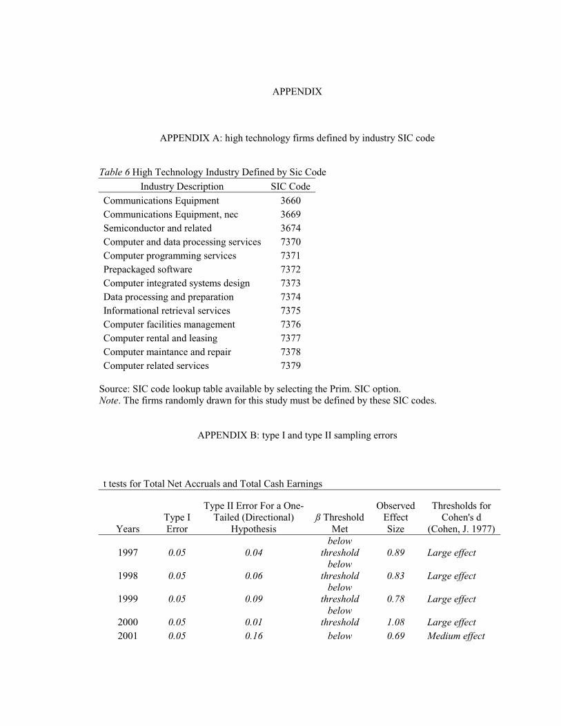
APPENDIX
APPENDIX A: high technology firms defined by industry SIC code
Table 6 High Technology Industry Defined by Sic Code
Industry Description SIC Code
Communications Equipment 3660 Communications Equipment, nec 3669 Semiconductor and related 3674 Computer and data processing services 7370 Computer programming services 7371 Prepackaged software 7372 Computer integrated systems design 7373 Data processing and preparation 7374 Informational retrieval services 7375 Computer facilities management 7376 Computer rental and leasing 7377 Computer maintance and repair 7378 Computer related services 7379
Source: SIC code lookup table available by selecting the Prim. SIC option. Note. The firms randomly drawn for this study must be defined by these SIC codes.
APPENDIX B: type I and type II sampling errors
t tests for Total Net Accruals and Total Cash Earnings
Years Type I Error
Type II Error For a One-Tailed (Directional)
Hypothesis ß Threshold
Met
Observed Effect Size
Thresholds for Cohen's d
(Cohen, J. 1977)
1997 0.05 0.04 below
threshold 0.89 Large effect
1998 0.05 0.06 below
threshold 0.83 Large effect
1999 0.05 0.09 below
threshold 0.78 Large effect
2000 0.05 0.01 below
threshold 1.08 Large effect 2001 0.05 0.16 below 0.69 Medium effect
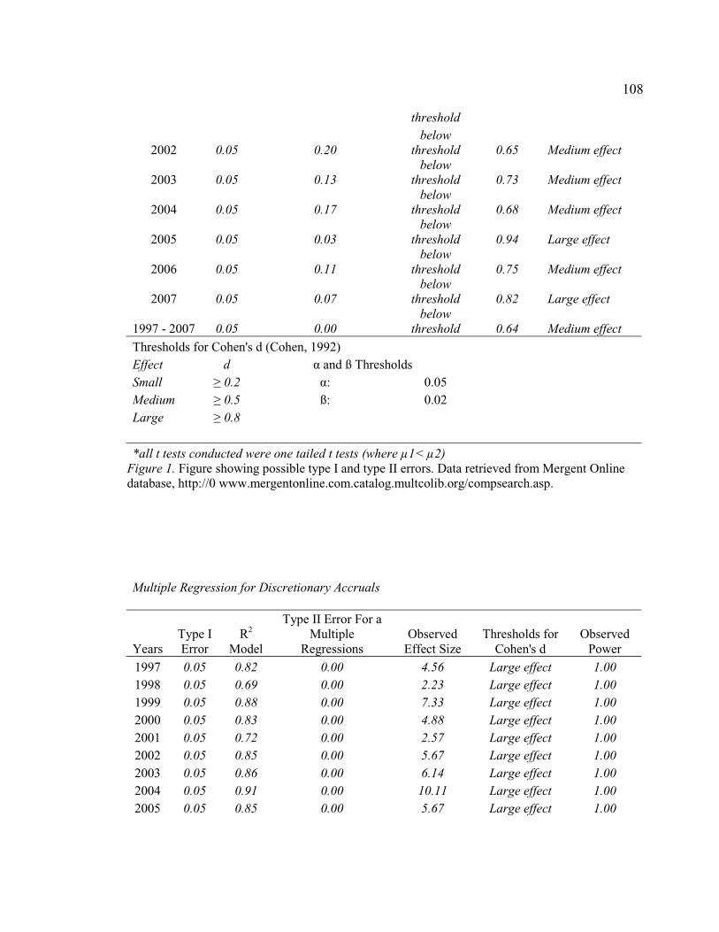
108
threshold
2002 0.05 0.20 below
threshold 0.65 Medium effect
2003 0.05 0.13 below
threshold 0.73 Medium effect
2004 0.05 0.17 below
threshold 0.68 Medium effect
2005 0.05 0.03 below
threshold 0.94 Large effect
2006 0.05 0.11 below
threshold 0.75 Medium effect
2007 0.05 0.07 below
threshold 0.82 Large effect
1997 - 2007 0.05 0.00 below
threshold 0.64 Medium effect
Thresholds for Cohen's d (Cohen, 1992) Effect d and ß Thresholds Small 0.2 : 0.05 Medium 0.5 ß: 0.02 Large 0.8
*all t tests conducted were one tailed t tests (where µ1< µ2) Figure 1. Figure showing possible type I and type II errors. Data retrieved from Mergent Online database, http://0 www.mergentonline.com.catalog.multcolib.org/compsearch.asp.
Multiple Regression for Discretionary Accruals
YearsType I Error
R2
Model
Type II Error For a Multiple
Regressions Observed
Effect Size Thresholds for
Cohen's d Observed
Power
1997 0.05 0.82 0.00 4.56 Large effect 1.00 1998 0.05 0.69 0.00 2.23 Large effect 1.00 1999 0.05 0.88 0.00 7.33 Large effect 1.00 2000 0.05 0.83 0.00 4.88 Large effect 1.00 2001 0.05 0.72 0.00 2.57 Large effect 1.00 2002 0.05 0.85 0.00 5.67 Large effect 1.00 2003 0.05 0.86 0.00 6.14 Large effect 1.00 2004 0.05 0.91 0.00 10.11 Large effect 1.00 2005 0.05 0.85 0.00 5.67 Large effect 1.00
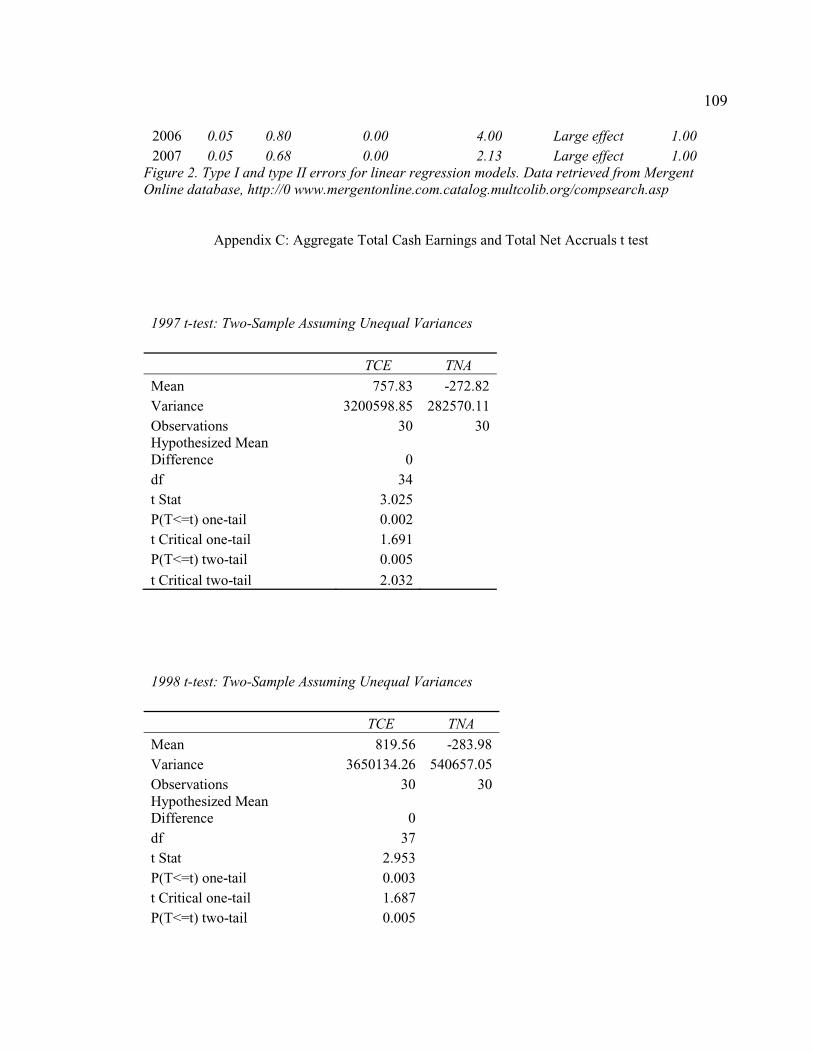
109
2006 0.05 0.80 0.00 4.00 Large effect 1.00 2007 0.05 0.68 0.00 2.13 Large effect 1.00
Figure 2. Type I and type II errors for linear regression models. Data retrieved from Mergent Online database, http://0 www.mergentonline.com.catalog.multcolib.org/compsearch.asp
Appendix C: Aggregate Total Cash Earnings and Total Net Accruals t test
1997 t-test: Two-Sample Assuming Unequal Variances
TCE TNA
Mean 757.83 -272.82Variance 3200598.85 282570.11Observations 30 30Hypothesized Mean Difference 0 df 34 t Stat 3.025 P(T<=t) one-tail 0.002 t Critical one-tail 1.691 P(T<=t) two-tail 0.005
t Critical two-tail 2.032
1998 t-test: Two-Sample Assuming Unequal Variances
TCE TNA
Mean 819.56 -283.98 Variance 3650134.26 540657.05 Observations 30 30 Hypothesized Mean Difference 0 df 37 t Stat 2.953 P(T<=t) one-tail 0.003 t Critical one-tail 1.687 P(T<=t) two-tail 0.005
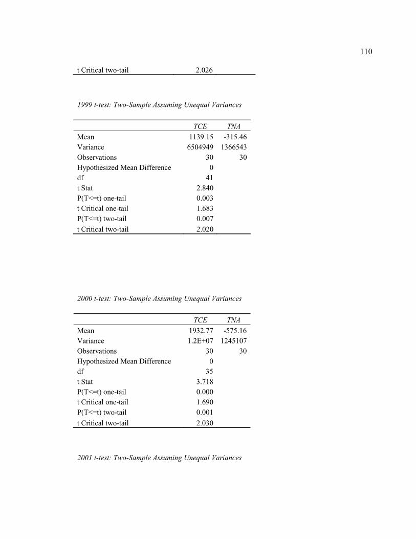
110
t Critical two-tail 2.026
1999 t-test: Two-Sample Assuming Unequal Variances
TCE TNA
Mean 1139.15 -315.46Variance 6504949 1366543Observations 30 30Hypothesized Mean Difference 0 df 41 t Stat 2.840 P(T<=t) one-tail 0.003 t Critical one-tail 1.683 P(T<=t) two-tail 0.007
t Critical two-tail 2.020
2000 t-test: Two-Sample Assuming Unequal Variances
TCE TNA
Mean 1932.77 -575.16 Variance 1.2E+07 1245107 Observations 30 30 Hypothesized Mean Difference 0 df 35 t Stat 3.718 P(T<=t) one-tail 0.000 t Critical one-tail 1.690 P(T<=t) two-tail 0.001
t Critical two-tail 2.030
2001 t-test: Two-Sample Assuming Unequal Variances
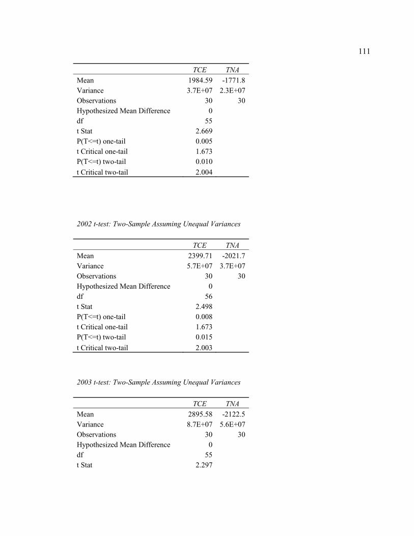
111
TCE TNA
Mean 1984.59 -1771.8 Variance 3.7E+07 2.3E+07 Observations 30 30 Hypothesized Mean Difference 0 df 55 t Stat 2.669 P(T<=t) one-tail 0.005 t Critical one-tail 1.673 P(T<=t) two-tail 0.010
t Critical two-tail 2.004
2002 t-test: Two-Sample Assuming Unequal Variances
TCE TNA
Mean 2399.71 -2021.7 Variance 5.7E+07 3.7E+07 Observations 30 30 Hypothesized Mean Difference 0 df 56 t Stat 2.498 P(T<=t) one-tail 0.008 t Critical one-tail 1.673 P(T<=t) two-tail 0.015
t Critical two-tail 2.003
2003 t-test: Two-Sample Assuming Unequal Variances
TCE TNA
Mean 2895.58 -2122.5 Variance 8.7E+07 5.6E+07 Observations 30 30 Hypothesized Mean Difference 0 df 55 t Stat 2.297
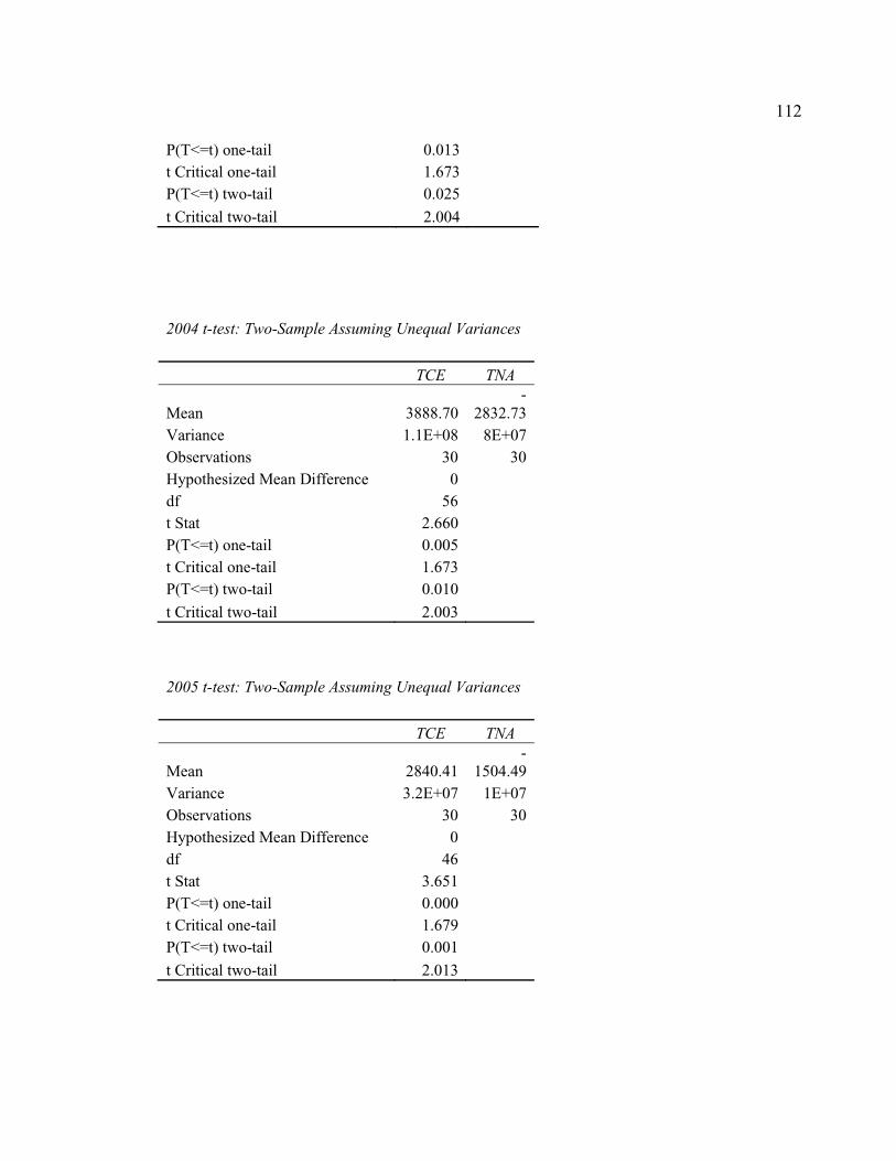
112
P(T<=t) one-tail 0.013 t Critical one-tail 1.673 P(T<=t) two-tail 0.025
t Critical two-tail 2.004
2004 t-test: Two-Sample Assuming Unequal Variances
TCE TNA
Mean 3888.70-
2832.73 Variance 1.1E+08 8E+07 Observations 30 30 Hypothesized Mean Difference 0 df 56 t Stat 2.660 P(T<=t) one-tail 0.005 t Critical one-tail 1.673 P(T<=t) two-tail 0.010
t Critical two-tail 2.003
2005 t-test: Two-Sample Assuming Unequal Variances
TCE TNA
Mean 2840.41-
1504.49 Variance 3.2E+07 1E+07 Observations 30 30 Hypothesized Mean Difference 0 df 46 t Stat 3.651 P(T<=t) one-tail 0.000 t Critical one-tail 1.679 P(T<=t) two-tail 0.001
t Critical two-tail 2.013
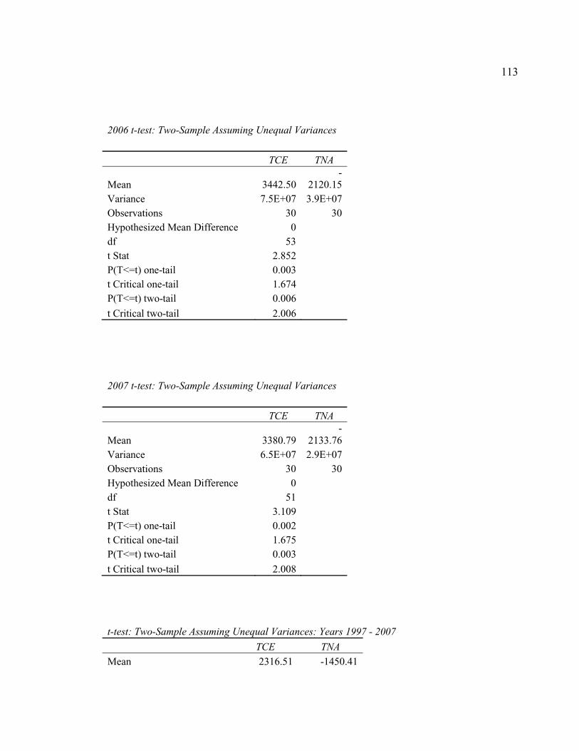
113
2006 t-test: Two-Sample Assuming Unequal Variances
TCE TNA
Mean 3442.50-
2120.15 Variance 7.5E+07 3.9E+07 Observations 30 30 Hypothesized Mean Difference 0 df 53 t Stat 2.852 P(T<=t) one-tail 0.003 t Critical one-tail 1.674 P(T<=t) two-tail 0.006
t Critical two-tail 2.006
2007 t-test: Two-Sample Assuming Unequal Variances
TCE TNA
Mean 3380.79-
2133.76 Variance 6.5E+07 2.9E+07 Observations 30 30 Hypothesized Mean Difference 0 df 51 t Stat 3.109 P(T<=t) one-tail 0.002 t Critical one-tail 1.675 P(T<=t) two-tail 0.003
t Critical two-tail 2.008
t-test: Two-Sample Assuming Unequal Variances: Years 1997 - 2007
TCE TNA
Mean 2316.51 -1450.41

114
Variance 44347539.39 25222379.93Observations 330 330Hypothesized Mean Difference 0 df 612 t Stat 8.204 P(T<=t) one-tail 0.000 t Critical one-tail 1.647 P(T<=t) two-tail 0.000
t Critical two-tail 1.964
APPENDIX D: Statistical Data Tables for Estimated Regression Equations
1997 Statistical Summary
SUMMARY OUTPUT
Regression Statistics Multiple R 0.906784685 R Square 0.822258465
Adjusted R Square 0.801749826
Standard Error 219.7655248 Observations 30
ANOVA
df SS MS F Significance
F
Regression 3 5809140.793 1936380.264 40.09327
4 6.75646E-10 Residual 26 1255719.033 48296.88588
Total 29 7064859.826
Coefficients Standard
Error t Stat P-value Lower 95%
Intercept 13.16848472 49.95308889 0.263617026 0.794153
1 -89.51155904

115
ATA 0.146520567 0.018999269 7.711905321 3.494E-
08 0.10746701
Sales – Rec -
0.147845307 0.083976192 -
1.760562167 0.090072
8 -0.32046084
GPPE -
0.078630479 0.030276976 -
2.597038672 0.015272
9 -0.140865694
Upper 95% Lower 95.0% Upper 95.0% Intercept 115.8485285 -89.51155904 115.8485285
ATA 0.185574124 0.10746701 0.185574124 Sales – Rec 0.024770227 -0.32046084 0.024770227
GPPE -
0.016395263 -0.140865694 -
0.016395263
1998 Statistical Summary SUMMARY OUTPUT
Regression Statistics Multiple R 0.836055057 R Square 0.698988058
Adjusted R Square 0.66425591
Standard Error 368.2747514 Observations 30
ANOVA
df SS MS F Significance
F
Regression 3 8188479.527 2729493.2 20.1251035
1 5.91566E-07 Residual 26 3526283.605 135626.29
Total 29 11714763.13
Coefficients Standard
Error t Stat P-value Lower 95%
Intercept 92.19335028 82.36271296 1.1193579 0.27322227
5 -77.1056292
ATA 0.122349795 0.024296051 5.0357893 3.05776E-
05 0.072408547
Sales – Rec 0.12400943 0.12387637 1.0010741 0.32601731
4-
0.130622092
GPPE -
0.101920287 0.036249553 -2.8116288 0.00925053
4-
0.176432309
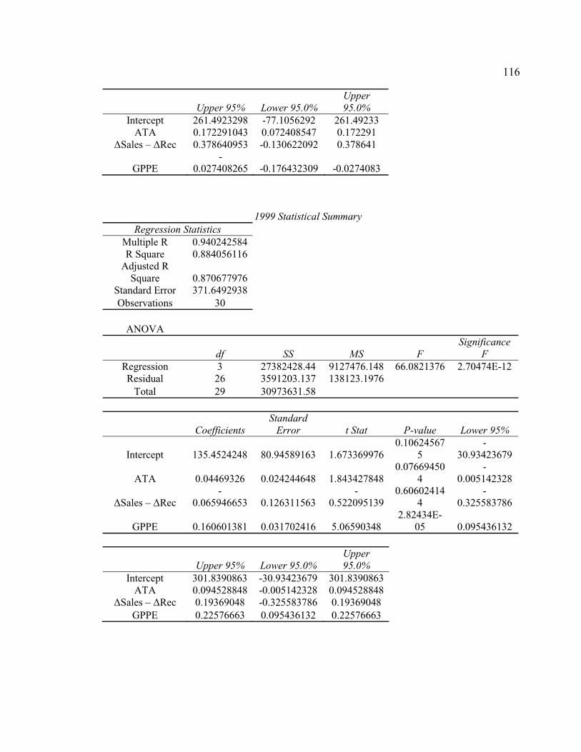
116
Upper 95% Lower 95.0% Upper 95.0%
Intercept 261.4923298 -77.1056292 261.49233 ATA 0.172291043 0.072408547 0.172291
Sales – Rec 0.378640953 -0.130622092 0.378641
GPPE -
0.027408265 -0.176432309 -0.0274083
1999 Statistical Summary Regression Statistics
Multiple R 0.940242584 R Square 0.884056116
Adjusted R Square 0.870677976
Standard Error 371.6492938 Observations 30
ANOVA
df SS MS F Significance
F Regression 3 27382428.44 9127476.148 66.0821376 2.70474E-12 Residual 26 3591203.137 138123.1976
Total 29 30973631.58
Coefficients Standard
Error t Stat P-value Lower 95%
Intercept 135.4524248 80.94589163 1.673369976 0.10624567
5-
30.93423679
ATA 0.04469326 0.024244648 1.843427848 0.07669450
4-
0.005142328
Sales – Rec -
0.065946653 0.126311563 -
0.522095139 0.60602414
4-
0.325583786
GPPE 0.160601381 0.031702416 5.06590348 2.82434E-
05 0.095436132
Upper 95% Lower 95.0% Upper 95.0%
Intercept 301.8390863 -30.93423679 301.8390863 ATA 0.094528848 -0.005142328 0.094528848
Sales – Rec 0.19369048 -0.325583786 0.19369048 GPPE 0.22576663 0.095436132 0.22576663
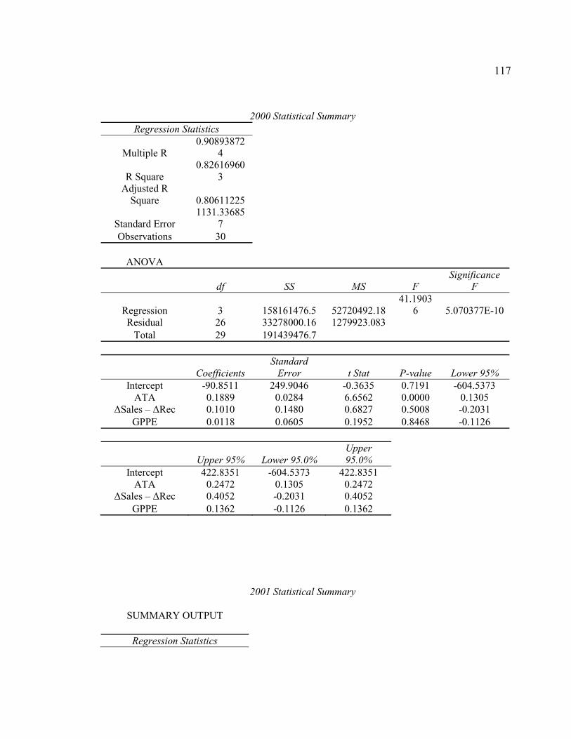
117
2000 Statistical Summary Regression Statistics
Multiple R 0.90893872
4
R Square 0.82616960
3Adjusted R
Square 0.80611225
Standard Error 1131.33685
7Observations 30
ANOVA
df SS MS F Significance
F
Regression 3 158161476.5 52720492.18 41.1903
6 5.070377E-10 Residual 26 33278000.16 1279923.083
Total 29 191439476.7
Coefficients Standard
Error t Stat P-value Lower 95% Intercept -90.8511 249.9046 -0.3635 0.7191 -604.5373
ATA 0.1889 0.0284 6.6562 0.0000 0.1305 Sales – Rec 0.1010 0.1480 0.6827 0.5008 -0.2031
GPPE 0.0118 0.0605 0.1952 0.8468 -0.1126
Upper 95% Lower 95.0% Upper 95.0%
Intercept 422.8351 -604.5373 422.8351 ATA 0.2472 0.1305 0.2472
Sales – Rec 0.4052 -0.2031 0.4052 GPPE 0.1362 -0.1126 0.1362
2001 Statistical Summary
SUMMARY OUTPUT
Regression Statistics

118
Multiple R 0.856447174 R Square 0.733501761
Adjusted R Square 0.702751965
Standard Error 2569.410076 Observations 30
ANOVA
df SS MS F Significance
F
Regression 3 472440381.5 157480127 23.8538734
6 1.24138E-07 Residual 26 171648571.6 6601868.1
Total 29 644088953.1
Coefficients Standard
Error t Stat P-value Lower 95%
Intercept -
761.5180935 574.6507213 -1.3251843 0.19663839
4-
1942.729557
ATA 0.358093657 0.052489498 6.8221963 3.05713E-
07 0.250199951
Sales – Rec -
0.129689135 0.406406222 -0.3191121 0.75219125
6-
0.965069081
GPPE -0.23757426 0.135269771 -1.7562997 0.09081169
4-
0.515625253
Upper 95% Lower 95.0% Upper 95.0%
Intercept 419.6933695 -1942.729557 419.69337 ATA 0.465987364 0.250199951 0.4659874
Sales – Rec 0.70569081 -0.965069081 0.7056908 GPPE 0.040476734 -0.515625253 0.0404767
2002 Statistical Summary
SUMMARY OUTPUT
Regression Statistics Multiple R 0.925317838 R Square 0.856213102
Adjusted R Square 0.839622306
Standard Error 2409.705392 Observations 30
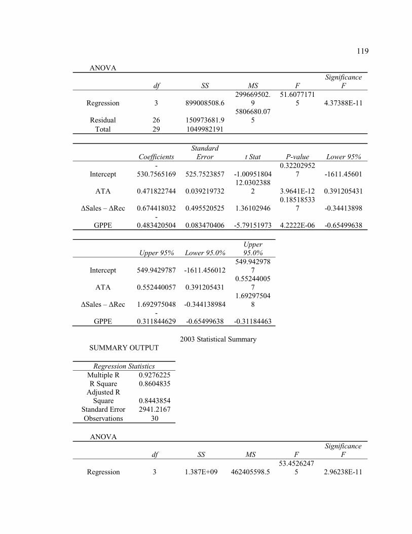
119
ANOVA
df SS MS F Significance
F
Regression 3 899008508.6 299669502.
951.6077171
5 4.37388E-11
Residual 26 150973681.9 5806680.07
5Total 29 1049982191
Coefficients Standard
Error t Stat P-value Lower 95%
Intercept -
530.7565169 525.7523857 -1.00951804 0.32202952
7 -1611.45601
ATA 0.471822744 0.039219732 12.0302388
2 3.9641E-12 0.391205431
Sales – Rec 0.674418032 0.495520525 1.36102946 0.18518533
7 -0.34413898
GPPE -
0.483420504 0.083470406 -5.79151973 4.2222E-06 -0.65499638
Upper 95% Lower 95.0% Upper 95.0%
Intercept 549.9429787 -1611.456012 549.942978
7
ATA 0.552440057 0.391205431 0.55244005
7
Sales – Rec 1.692975048 -0.344138984 1.69297504
8
GPPE -
0.311844629 -0.65499638 -0.31184463
2003 Statistical Summary SUMMARY OUTPUT
Regression Statistics Multiple R 0.9276225 R Square 0.8604835
Adjusted R Square 0.8443854
Standard Error 2941.2167 Observations 30
ANOVA
df SS MS F Significance
F
Regression 3 1.387E+09 462405598.5 53.4526247
5 2.96238E-11

120
Residual 26 224919648 8650755.705 Total 29 1.612E+09
Coefficients
Standard Error t Stat P-value Lower 95%
Intercept -881.75872 631.85887 -
1.395499468 0.17467076
4 -2180.563226
ATA 0.3432068 0.0557855 6.152262274 1.66437E-
06 0.228538169
Sales – Rec 4.1760537 0.9999854 4.176114678 0.00029495
6 2.120554315
GPPE -0.6182182 0.0971368 -
6.364406311 9.68199E-
07 -0.817885827
Upper 95% Lower 95.0%
Upper 95.0%
Intercept 417.04578 -2180.5632 417.0457808 ATA 0.4578755 0.2285382 0.45787552
Sales – Rec 6.2315532 2.1205543 6.231553162
GPPE -0.4185506 -0.8178858 -
0.418550622
2004 Statistical Summary SUMMARY OUTPUT
Regression Statistics Multiple R 0.955281106 R Square 0.912561992
Adjusted R Square 0.902472991
Standard Error 2772.562658 Observations 30
ANOVA
df SS MS F Significance
F
Regression 3 2085922698 695307566.1 90.4511755
9 7.00415E-14 Residual 26 199864696.1 7687103.695
Total 29 2285787394
Coefficients Standard
Error t Stat P-value Lower 95%

121
Intercept -
1021.519817 635.2848874 -
1.607971223 0.11991887
2-
2327.366592
ATA 0.584184789 0.046574439 12.54303423 1.56188E-
12 0.488449658
Sales – Rec -
0.504481638 0.716209871 -
0.704376829 0.48745986
9-
1.976672098
GPPE -
0.527781104 0.090699055 -
5.819036394 3.93125E-
06 -0.71421568
Upper 95% Lower 95.0% Upper 95.0%
Intercept 284.3269581 -2327.366592 284.3269581 ATA 0.679919919 0.488449658 0.679919919
Sales – Rec 0.967708822 -1.976672098 0.967708822
GPPE -
0.341346527 -0.71421568 -
0.341346527
2005 Statistical Summary SUMMARY OUTPUT
Regression Statistics Multiple R 0.913243949 R Square 0.83401451
Adjusted R Square 0.814862338
Standard Error 1321.027929 Observations 30
ANOVA
df SS MS F Significance
F
Regression 3 227982141.5 75994047.16 43.5467326
2 2.79381E-10 Residual 26 45372984.55 1745114.79
Total 29 273355126
Coefficients Standard
Error t Stat P-value Lower 95%
Intercept 77.50218887 288.726343 0.268427841 0.79048837
5 -515.983303
ATA 0.19621025 0.019843618 9.887826233 2.68003E-
10 0.155421109
Sales – Rec -
0.314843772 0.492585507 -
0.639165725 0.52830663
2-
1.327367772 GPPE - 0.047659317 - 0.02525916 -
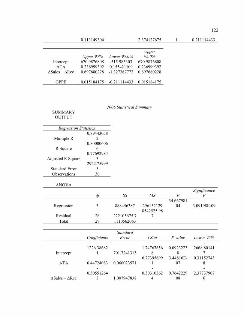
122
0.113149304 2.374127675 1 0.211114433
Upper 95% Lower 95.0% Upper 95.0%
Intercept 670.9876808 -515.983303 670.9876808 ATA 0.236999392 0.155421109 0.236999392
Sales – Rec 0.697680228 -1.327367772 0.697680228
GPPE -
0.015184175 -0.211114433 -
0.015184175
2006 Statistical Summary SUMMARY
OUTPUT
Regression Statistics
Multiple R 0.89443058
2
R Square 0.80000606
6
Adjusted R Square 0.77692984
3
Standard Error 2922.75999
5Observations 30
ANOVA
df SS MS F Significance
F
Regression 3 888456387 296152129 34.667981
04 3.09198E-09
Residual 26 222105675.7 8542525.98
7Total 29 1110562063
Coefficients Standard
Error t Stat P-value Lower 95%
Intercept
-1226.38682
1 701.7241313
-1.74767656
80.0923223
8
-2668.80141
7
ATA 0.44724083 0.066023571 6.77395699
13.44816E-
070.31152743
8
Sales – Rec
-0.30551264
3 1.007947838
-0.30310362
40.7642229
08
-2.37737907
6
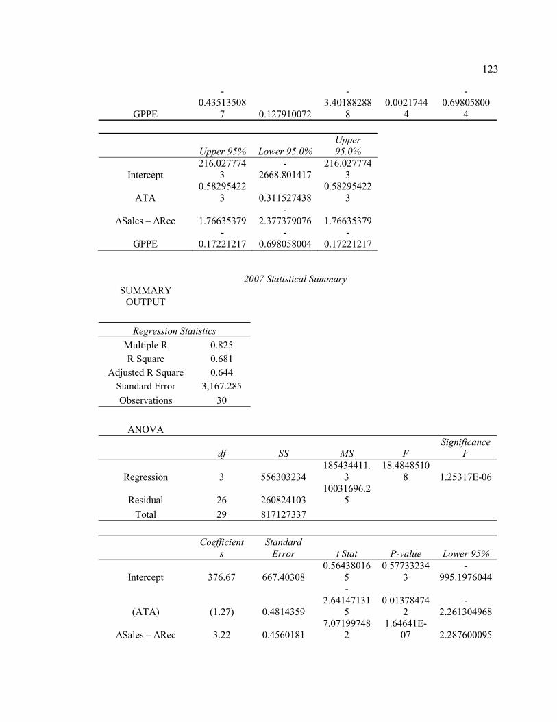
123
GPPE
-0.43513508
7 0.127910072
-3.40188288
80.0021744
4
-0.69805800
4
Upper 95% Lower 95.0% Upper 95.0%
Intercept 216.027774
3-
2668.801417 216.027774
3
ATA 0.58295422
3 0.311527438 0.58295422
3
Sales – Rec 1.76635379 -
2.377379076 1.76635379
GPPE -
0.17221217 -
0.698058004 -
0.17221217
2007 Statistical Summary SUMMARY
OUTPUT
Regression Statistics
Multiple R 0.825 R Square 0.681
Adjusted R Square 0.644 Standard Error 3,167.285
Observations 30
ANOVA
df SS MS F Significance
F
Regression 3 556303234 185434411.
318.4848510
8 1.25317E-06
Residual 26 260824103 10031696.2
5
Total 29 817127337
Coefficients
Standard Error t Stat P-value Lower 95%
Intercept 376.67 667.40308 0.56438016
50.57733234
3-
995.1976044
(ATA) (1.27) 0.4814359
-2.64147131
50.01378474
2-
2.261304968
Sales – Rec 3.22 0.4560181 7.07199748
21.64641E-
07 2.287600095
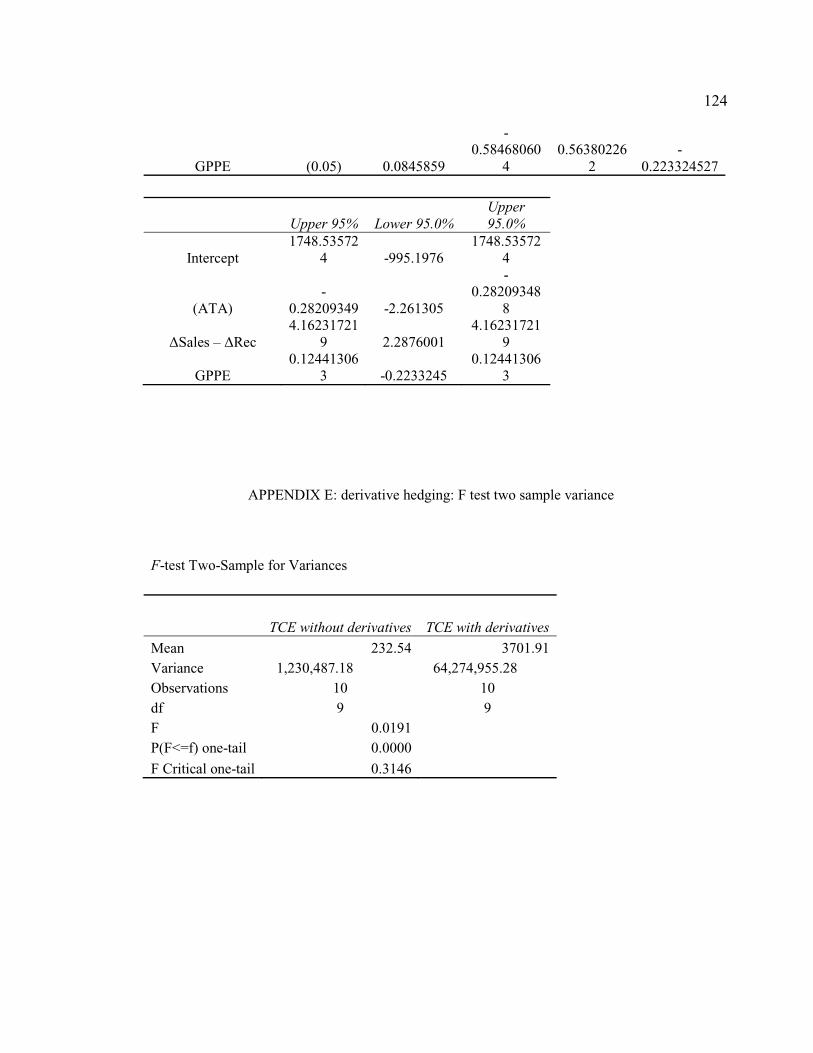
124
GPPE (0.05) 0.0845859
-0.58468060
40.56380226
2-
0.223324527
Upper 95% Lower 95.0% Upper 95.0%
Intercept 1748.53572
4 -995.1976 1748.53572
4
(ATA) -
0.28209349 -2.261305
-0.28209348
8
Sales – Rec 4.16231721
9 2.2876001 4.16231721
9
GPPE 0.12441306
3 -0.2233245 0.12441306
3
APPENDIX E: derivative hedging: F test two sample variance
F-test Two-Sample for Variances
TCE without derivatives TCE with derivatives
Mean 232.54 3701.91 Variance 1,230,487.18 64,274,955.28 Observations 10 10df 9 9F 0.0191P(F<=f) one-tail 0.0000
F Critical one-tail 0.3146

CURRICULUM VITAE
Margot Geagon 327 NW Gina Way, Apt 230, Aloha, OR 97006 Email: [email protected] Phone: (503) 467-6135 PROFILE This is a profile of a high caliber finance and economic professional with strong a strong background in financial analysis, econometrics, and statistics.
EDUCATION Ph.D. Walden University, Applied Management Decision Sciences Major: Finance Support Area: Strategic Finance Dissertation Title: Earnings Management with Derivatives and the use of Accounting Accruals Dissertation Chairman: Dr. Thomas Spencer
M.B.A. Marylhurst University Graduate School, June 2003. Thesis Title: An Analytical Approach to Valuing Human Capital Investments with Real Options Concentration: Finance
M.P.A. Portland State University Hatfield School of Government, August 2002. Thesis Title: Performance Measurement in the Public Sector: Evaluating the Subjective Benefits of Public Service Concentration: Program Evaluation
M.F.M. Portland State University Hatfield School of Government (Masters Endorsement), August 2002. Thesis Title: Disincentives to Efficiency: Public Sector Budgeting Structure Concentration: Public Sector Financial Management B.A. Western New Mexico University, School of Management, May 1982. Received dual degrees in magazines and marketing management Concentration: Business Administration: Finance
TEACHING EXPERIENCE Adjunct Professor of Economics, Warner Pacific University, School of Business, Summer and Fall Sessions 2005. Adjunct Professor of Finance, Warner Pacific University, School of Business, Summer and Fall Sessions 2005. Undergraduate Teaching: Microeconomics, Macroeconomics & Corporate Finance, Primary teaching areas: Introduction to Business, Introduction to Management course. Average class size of 40.
HIGHLIGHTS OF WORK EXPERIENCE Business Strategist, Silver City Trading Company, 1994-1999 Managed operational staff and reduced operational costs by 32% by creating operational policies. Created financial statements and capital budgeting modules for financial reporting and planning. Created mission based budgeting standards
126
Cost Accounting Manager, Compact Controls, 1999-2004 Supervised the Accounting Department and implemented cost rollups for manufactured and purchased materials. Prepared trial balances for months end and closed the books for all accounts. Problem solved variances between the general ledger and subsidiary ledgers. Reduced process times by 17% by performing time studies and establishing manufacturing standards.
Financial Consultant, Nike, 2001-2002 Formulated Descriptive Statistical Standards for Cost Accounting Created an Economic Order Quantity Standard for Purchasing: Team Sports Reduced the cost of inventory moves through all associated inventory accounts by 27%.
Financial Consultant, Oregon Health Sciences University: Cancer Institute, 2002-2003 Provided financial consulting for the Bioinformatics Core Assisted in the formulation of the 2003-2008 Master NIH Grant Created Funds Flows Statements for Clinical Trials
Cost Accountant III, Regence Blue Cross Blue Shield of Oregon, 2005-2008. Created Medical, Dental, and Drug statistics for Claims, Contracts, Members, and Groups for all Regence Plans and TRG [The Regence Group] Analyzed and managed Plan and TRG Operational Accounts. Performed Analysis and Problem Solved Accounting Discrepancies in Operational Activities for 5 divisions [Actuarial, Underwriting, Finance, Human Resources, and Membership Services]
MEMBERSHIPS & AFFILIATIONS Professional: Member of the Emerging Markets Advisory Board for Regence BCBS Member of the American Finance Association Member of the American Statistical Association: Oregon Charter
RESEARCH Hedging in International Markets, 2004Abstract:
In this explorative study, an investigation of theoretical options models used in international finance is evaluated to acquire knowledge that explains why global firms support decisions to employ financial hedges. The findings of this study suggest International investing through the utilization of derivative contracts may minimize the firm’s exposure to systematic risk. An illustration of markets conversion is presented in this study to provide an explanation of the inherent volatility of international markets and the increased level of systematic risk.
Application Errors of Financial Derivatives, 2005
Abstract:
The premise of this study is grounded on an in-depth evaluation of finance strategies from the context of current international financial risk management. The scope includes the analysis of financial derivatives that are valued on the performance of other underlying investment
127
instruments. The range of this analysis includes derivatives such as (a) options; (b) futures; (c) swaps, and (d) commodity futures. In this evaluation, each derivative design has been analyzed in terms of inherent strengths and weaknesses when applied to real life situations of uncertainty.
Capital Budgeting Theory in Practice, 2006
Abstract:
An investigation of theoretical finance models used in capital budgeting is presented in this research study. This analysis is completed to elucidate the rationale of the twenty-first century financial manager attempting to make vital corporate decisions based on educated guesses and corporate rules of thumb. Capital budgeting decisions involve the largest tangible investments of any firm and require a more robust framework of analysis. The evaluation approach of this study is established by critically analyzing capital budgeting theories, and through the assessment of existing theoretical propositions and hypotheses that comprise strategic capital budgeting.
Implications of Derivative Applications, 2006
Abstract:
The implications of derivative applications can be devastating and can create risk barriers within international markets. This study provides an in-depth evaluation widely accepted financial models including (a) Black-Scholes model; (b) the stochastic-interest-rate option model created by Merton; (c) Amin and Jarrow’s discrete path-independent model, and (d) the Cox and Ross jump and diffusion processes model. The objective of this investigation is to identify the best hedging strategy by evaluating each derivative model with the intent to expose the effectiveness of each model in terms of pricing errors.
Capital Budgeting Misconceptions in the Workplace, 2007
Abstract:
Capital Budgeting is a tremendously vital aspect of a firm's financial structure. Many business professional may neglect the importance of this particular area of business due in large part to the total proportion of capital assets this area represents. It is true, capital assets usually represent a smaller portion of a firm’s total assets however, unlike current assets; capital assets are long-term investments that require long-term commitments. When a firm purchases a capital asset, the firm exposes itself to risks associated with a long-term investment. If for example, the firm makes a mistake in purchasing a capital asset the firm must live with that mistake for a long period of time. It is clear capital budgeting is of the utmost importance to any firm.
The objective of this study is to provide an in-depth knowledge base of the most widely used asset pricing models in strategic capital budgeting including the (a) payback method; (b) net present value; (c) internal rate of return, and (d) capital asset pricing model (CAPM). In exploration, each variable that embodies the theory of the CAPM has been analyzed in terms of inherent strengths and weaknesses when applied to real life situations of uncertainty.
128
Capital Rationing with Real Options and Linear Programming, 2007
Abstract:
This investigation explores the implications of capital budgeting theory and the implementation of widely used budgeting models utilized for capital rationing, mutually exclusive and independent investment projects. Particular models include the internal rate of return (IRR); modified IRR; net present value; profitability index technique; and capital asset pricing model.
Real options; linear programming; and optimization models are introduced as models that maximize capital asset allocations more effectively in situations of uncertainty. The alternative models introduced in this study have been tested in financial applications. Recommendations are provided based on the findings of the study that include the elimination of obsolete financial models introduced in most business schools.
ResidenciesWinter Session, Dallas, TX 2006 Spring Session, Los Angeles, CA 2005 Summer Session, Seattle, WA 2004


![[Derivatives Consulting Group] Introduction to Equity Derivatives](https://img.dokumen.tips/doc/110x75/5525eed15503467c6f8b4b12/derivatives-consulting-group-introduction-to-equity-derivatives.jpg)