Evaluating Early Childhood Policies: An Estimable Model ofFamily Child Investments

Rodrigo Azuero∗

Link to latest version: http://rodrigoazuero.com/files/jmp.pdf

November 16, 2016

Abstract

There is extensive evidence showing that skills developed early in life have important consequencesfor adult life outcomes. Such findings have motivated a large literature analyzing the production ofskills in young children. However, little is known about how families make decisions about invest-ments in their children. In this paper, I estimate a production function of skills in young children,nested within a collective model of household behavior, using data from Chile. The estimated modelis used to simulate the effects of various policies aimed at increasing skills of children in disadvan-taged households that are popular in developing countries. The data reveals substantial disparities inthe skills of poor and rich children when they are five years old. I find that to close this gap in skills, itis more effective to design policies that subsidize the acquisition of skill-enhancing goods for childrenthan policies providing unconditional cash transfers or childcare subsidies.

1 Introduction

Research in medicine, psychology and economics shows that skills shaped during the first years of lifehave significant consequences for adult life outcomes.1 This fact has motivated a large amount of re-search in economics aimed at understanding the skill formation process. The results of these studiesallow a better understanding of the key inputs that promote skills in young children.2 For instance, theyshowed that parenting and general family environment are among the most relevant inputs in the pro-duction of skills (J. Heckman & Mosso, 2014; Schoellman, 2014).

Gaps in skills between rich and poor children emerge very early in life, even before they start theirformal education. Duncan and Magnuson (2013) find that differences in reading and math test scoresbetween children in the top and bottom quartile of the income distribution are about one standard de-viation when they start kindergarten in the US. Schady et al. (2015) report similar quantitative results

∗University of Pennsylvania. This research is partially supported by the Eunice Kennedy Shriver National Institute of ChildHealth and Human Development (NICHD R01HD065436) grant on “Early Child Development Programs: Effective Interven-tions for Human Development”. Funding from the Judith Rodin Fellowship and the Penn Institute for Economic Research isacknowledged. I am indebted to the members of my committee, Petra Todd, Andrew Shephard and Jere Behrman, for theiradvice and support in developing this project. Special thanks to Aureo de Paula, Chris Flinn, Holger Sieg, Hanming Fang,Sergio Urzua, Flavio Cunha and seminar participants at ECONCON (2015) and EMCON (2016) for their comments, whichsignificantly improved the quality of this paper. I am grateful to the Centro Nacional de Microdatos for its support with thedataset as well as to Daniela Marshall and Alejandra Abufhele for their guidance and help with the data. The online appendixis available in the following link: http://rodrigoazuero.com/files/OnlineAppendix.pdf

1For a review, see Conti and Heckman (2012)2See, for example, Cunha, Heckman, and Schennach (2010)

1

for five Latin American countries, using a vocabulary test for children younger than five. Research inneuroscience shows that malleability of skills decreases with age (Nelson & Sheridan, 2011). To closegaps in skills between the rich and poor population, we need to develop policies addressing this issueduring early childhood.

The goal of this paper is to evaluate the effects that early childhood policy interventions have on theskill gaps between rich and poor children. Knowledge of the skill production function is not enough toassess the effectiveness of policies aimed at improving children’s skills. Families administer resourcesand make the relevant decisions that determine the allocation of inputs for young children. Family in-vestments in children might react to policy interventions. To analyze how early childhood policies affectresources allocated to children and skill formation, I develop and estimate a skill production functionnested within a collective model of household behavior using data from Chile. I evaluate the effects ofcash transfers, childcare subsidies and in-kind transfers, which are transfers of goods that can be used inthe skill formation process in children (for example, books, toys, puzzles, and guides about early child-hood development). I find that in-kind transfers provide the most cost-efficient way to reduce the gapsin skills between rich and poor children.

This paper makes several contributions to the literature on family investments and child outcomes.First, there are not many papers estimating a model of household behavior where parents allocate timeand money to their children to enhance their skills (Bernal, 2008; Del Boca, Flinn, & Wiswall, 2014, 2016;Gayle, Golan, & Soytas, 2015). This is the first paper that empirically evaluates and compares the effectsthat cash transfers, childcare subsidies and in-kind transfers have on the gaps in skills between rich andpoor children.

Cash transfer programs have been widely implemented in developing countries. In Latin America,they constitute the largest social assistance programs, covering millions of households in countries suchas Brazil, Mexico, Nicaragua and Colombia (Fiszbein, Schady, & Ferreira, 2009). Additionally, govern-ments in both developing and developed countries have invested a large amount of resources in theprovision of preschool services. In 2011, the United States federal government spent US$ 8.1 billionon Head Start, the largest childcare program. In Chile, firms employing more than twenty people arerequired to provide childcare services to their female employees. During the last ten years, Chile hasexperienced a massive expansion in the number of childcare providers. Between 2006 and 2010, the net-work of childcare providers increased its capacity, measured as the maximum number of children forwhom the system could provide coverage, by approximately 500% (U. Chile, 2010).

A limitation of cash transfers is that it is not possible not possible to guarantee that a given amount ofmoney will be spent on goods that can actually translate into better child outcomes. However, when thetransfer is done in-kind via puzzles, toys, guides about child development, or specific types of food thatcan improve children’s nutritional status, governments can enrich the environment and thus promoteskills for children. These transfers are usually implemented by governments through their early child-hood development programs. Currently, the program “Chile Grows with You”3, which is the main earlychildhood program in Chile, delivers a basket of goods to families for such purposes. Given the large

3In Spanish, “Chile Crece Contigo”.

2

amount of resources that governments spend on enriching childhood environments, and given the factthat events during childhood heavily influence adult outcomes, it is important to understand the mostcost-effective way of allocating these resources, whether through cash transfers or in-kind.

This paper also contributes to the literature of household decisions and child outcomes by allowingindividual family members to have different preferences. First, modeling household behavior throughthe collective approach has proven to result in better empirical predictions than the unitary framework.Second, from a policy perspective, it is common to see interventions targeting individual householdmembers. For instance, most cash transfer programs in developing countries state as an explicit condi-tion that, in households with children, mothers should be the sole recipients of such subsidies (Fiszbeinet al., 2009). It is often argued that mothers have stronger preferences for meeting the needs of childrenand therefore cash in the hands of mothers translates into better child outcomes (Blundell, Chiappori,& Meghir, 2005). By estimating a technology of skill formation within a collective setting, I am able toassess the extent to which targeting individual household members translates into different child out-comes.

The dataset used in this article allows me to overcome some empirical limitations that the literature haspreviously faced. For instance, studies have shown that parental skills largely determine children’s skills(J. Heckman & Mosso, 2014). By having information on parental IQ tests and personality assessments,I am able to incorporate parental skills into my estimation strategy. Additionally, we know that there isa multiplicity of skills that are relevant to determining adult life outcomes (Cunha et al., 2010). I incor-porate multiple measures of skills across various dimensions, such as motor, communication, cognitiveand behavioral abilities in children.

The productivity of time investments in children depends on the interactions between parents andchildren. Fiorini and Keane (2014) find that, when evaluating information about the time parents spendwith children, it is important to differentiate among activities such as watching TV, educational activi-ties with parents, and educational activities with other adults, as each of these translates differently intoskill formation. By using data on the frequency with which parents perform fourteen different types ofactivities with their children, I am able to incorporate not only the time component but also the qualityof interactions between parents and children. Additionally, I use geocoded datasets matching all thenationally registered childcare providers with the households in the survey to obtain information aboutthe cost of investing in children. Households that have a relatively large supply of childcare serviceswithin their neighborhood might, in principle, find it easier to invest in their children through preschoolservices. Additionally, households living in neighborhoods with a large number of preschool providersmight live in a children friendly environment, where the availability of goods to increase skills in chil-dren is relatively high.

The survey used for this study is the Early Childhood Longitudinal Survey from Chile (ECLS). Thissurvey was developed with the goal of precisely characterizing the skill formation process in children.Therefore, I am able to provide a unique empirical description of parental investments in children. I ob-serve the weekly frequency of consumption of different types of food for children, as well as availabilityof toys, books, and puzzles, as well as a precise characterization of which specific skills such elements

3

might promote.This paper also makes a methodological contribution to the estimation of dynamic microeconomic

models with unobserved and continuous state variables. By implementing an efficient simulation-basedestimator using particle filtering techniques from the machine learning and financial econometrics lit-erature (Murphy, 2012; Creal, 2012), I propose a feasible computational approach for dealing with thehigh dimensionality integration problem that arises in such models. Moreover, this is the first paperin the literature of household choices and child development that estimates a technology of skill for-mation through a dynamic latent-factor approach a-la Cunha et al. (2010). This allows me to obtainnon-parametric identification of the skill production technology by using a large number of skill mea-sures. Most of the prior research analyzing the child skill formation process uses data from the UnitedStates. By analyzing this process in the context of Chile, I bring new insights regarding the skill forma-tion process and the effect that policies and programs have on the skills of children in a situation wherepoor children face significant disadvantages.

There has been extensive study of the theoretical properties of the collective model of household behav-ior related to goods that are “public” within the context of the household (Blundell et al., 2005; Chiappori& Donni, 2009; Browning, Chiappori, & Weiss, 2014). However, there are still very few empirical studies(Cherchye, De Rock, & Vermeulen, 2012). The main challenge of estimating collective models of house-hold behavior is that of identifying the bargaining power, or Pareto weight, of each household member.The common approach to deal with this issue is to observe the consumption of private goods within thehousehold, such as gender-specific clothing, together with distribution factors. Distribution factors arevariables that affect the final outcomes of households, exclusively by modifying the bargaining power ofeach member. Examples of distribution factors commonly used in the literature include local sex ratios,the proportion of non-labor income in the household that is in the hands of women, and the differencesin ages between husband and wife. This approach assumes that the good observed is purely private (i.e.,a husband does not care about his spouse’s clothing) and that all the bargaining power is explained bythe consumption of a single good.

In this paper, I propose a new framework for estimating collective models of household behavior. I useinformation from questionnaires related to female empowerment and gender roles to assess the bargain-ing power of each household member. The use of answers to such questions, combined with exogenousvariation in the distribution factors, allows me to identify the Pareto weight of each member in the house-hold. Following such an identification strategy, I am also able to allow for unobserved heterogeneity.

The data from test scores show significant large gaps in skills between rich and poor children at age5. The skill gap between children in the lowest quintile of the income distribution and children in thehighest quintile, are in between 0.3 and 0.7 standard deviations in tests measuring cognitive abilities,socio-emotional development, and vocabulary skills, among others. These inequalities are mostly ex-plained by differences in parental skills and monetary investments. Additionally, , the model parameterestimates show that fathers’ time spent with children is 50% as productive as mothers’ time and thatmothers have stronger preferences for children. However, the higher productivity and the stronger pref-erences for children do not by themselves explain the observed disparities in time investments between

4

mothers and fathers. Given that women have lower bargaining power, they contribute more to the pro-vision of public goods within the household. This particular mechanism explains 15% of the differencesin time investments between mothers and fathers.

I use the estimated behavioral model to simulate the effects that cash transfer programs, free child-care subsidies, and in-kind transfers have on the skill gap between rich and poor children. Althoughless prevalent than the other two programs, in-kind transfers are currently being implemented in Chilethrough the “Chile Grows with You” program. I find that in-kind transfers are much more effective thanthe other alternatives when it comes to closing the gaps in skills between rich and poor children.

The remainder of this article is structured as follows: In Section 2, I briefly review the literature in orderto identify the main contributions of this article. I describe the data in Section 3. In Section 4, I presentsome preliminary evidence motivating the economic model, which will be described in Section 5. Theestimation procedure, together with the relevant identification arguments, are introduced in Section 6.The main results of the paper are in Section 7. I summarize the main points of this paper in Section 8.

2 Review of the literature

This article is related to four areas of the literature in economics. First of all, this paper is related tothe literature analyzing how household behavior affects the production of skills in children. One of themost important decisions families make relevant to the production of child skills, is that of labor supply.As household members increase their participation in the labor market, this will bring more monetaryresources to the household but will reduce the amount of time parents interact with their children. Forthis reason, the impact of labor force participation on the skills of children is not obvious at first glance.

The question of how labor supply decisions affect the production of skills in young children has beenexplored in the literature. Bernal (2008) estimates a structural model of female labor force participation,taking into account that skills are affected by family income and also by the total amount of time thatmothers interact with their children. Due to data limitations, she does not incorporate paternal time as apotential input in the skills of children. Taking into account the overall effect of an increase in income buta decrease in the amount of time that mothers interact with their children,Bernal (2008) finds that oneyear of full employment decreases the skills in children by approximately 0.13 of a standard deviation.

Del Boca et al. (2014) extend the results of Bernal (2008) and take into account that both parents partic-ipate in the production of skills. The authors estimate a unitary dynamic model of household behaviorwhere each parent allocates time to labor market, leisure, or interaction with their children. Additionally,they incorporate decisions about how much money to allocate to monetary investments in children ver-sus consumption. Results show that, when mothers increase time spent in the labor force, the potentialnegative effect is not only alleviated by the increase in the amount of resources due to wages but also bythe fact that the father starts to spend more time with the children at home. One of the main conclusionsis that time of both fathers and mothers are relatively more important than monetary investments in theproduction of child skills. Gayle et al. (2015) extends the modeling framework of Del Boca et al. (2014)to incorporate endogenous fertility. However, they do not observe test scores in their data or monetary

5

investments by parents and ignore the role of preschool education.The article that is most related to this paper is Del Boca et al. (2014). This paper extends Del Boca et

al. (2014) in several ways. First, I incorporate the decision to enroll a child in preschool services. This isimportant given that subsidizing preschool is one of the most important policies to improve the condi-tions in which children develop, and to increase female labor force participation.

Additionally, a major point in which this article departs from the analysis of Del Boca et al. (2014) isthat I estimate a collective model of household behavior, allowing parents to have different preferences,as opposed to using the unitary approach. There are two reasons why this is important. First of all,in most developing countries, cash transfers to families with children are given to their mothers, moti-vated by the findings that cash in the hands of women seems to translate into better child outcomes thancash in the hands of men (Duflo, 2000; Attanasio & Lechene, 2014; Thomas, 1994). To assess the effectthat targeting individual household members has on child outcomes and to identify the extent to whichadditional resources should be spent on targeting, I estimate a collective model of household behavior,where parents have different preferences. Additionally, the empirical regularity that there is a positivecorrelation between women’s empowerment and child development (Haddad, Hoddinott, Alderman, etal., 1997) cannot be explained by considering the household as a single entity with one utility function.This has motivated a large literature analyzing the relationship between female empowerment and childoutcomes (Doepke & Tertilt, 2014). By modeling household behavior using a collective approach, I amable to assess the extent to which empowering women translate into better child outcomes.

Third, this is the first paper that estimates a model of parental investments and child outcomes usingobservations not only on time investments but also on in-kind investments. The data I use includes adetailed description of the environment in which children grow. Enumerators who visited the house-holds were trained to provide a precise characterization of the child’s environment. For instance, notonly I do observe the availability of toys, but also whether the toys are ideal for the promotion of specificskills, such as motor skills or behavioral skills, or toys that help develop free expression in children. I ob-serve the availability puzzles, costumes, and children’s books and music. Additionally, I have detailedinformation about the frequency with which children consume different types of food, such as fruits,vegetables, and fish, among others. This information is used to assess the effect of in-kind investments.

The dataset I use allows me to incorporate several facts about the skill formation process in childrenthat were not incorporated in Del Boca et al. (2014). First of all, there is a consensus in the literature thatskills are multiple (emotional, physical, cognitive). In this paper, rather than using one cognitive testscore as a measure of skills, I use various indicators of motor development, cognitive achievement andemotional attainment in young children as broad measures of skills. Additionally, an important elementin the skill formation process is their dependence on parental skills (Francesconi & Heckman, 2016). Ig-noring parental skills when estimating a production function might bias the effect of other inputs, suchas time or in-kind investments. I overcome this limitation by using various assessments of cognitiveachievement and personality traits of parents.

By implementing a dynamic latent factor structure in the estimation of the skill production function forchildren, I am able to obtain non-parametric identification of the skill production function in children.

6

This is accomplished by using identification results from the literature of skill formation (Cunha et al.,2010). Because of that, the results of the estimation are less sensitive to the specific parametric formassumed for the skill formation technology, and the bias arising from measurement error is reduced,making the results more robust. This, along with the fact that a latent factor structure can be inter-preted as unobserved heterogeneity (Carneiro, Hansen, & Heckman, 2003) and potentially improves theaccuracy of the estimates, has made factor analysis a popular tool to get accurate estimates of the skillproduction function (Cunha et al., 2010; Cunha & Heckman, 2008; J. J. Heckman, Stixrud, & Urzua, 2006).This paper is the first to estimate the production function of skills via a latent-factor approach, nestedwithin a collective model of household behavior.

The second area of related literature the empirical implementation of collective models of householdbehavior. The income pooling assumption establishes that, in a household composed of various mem-bers, it does not make a difference if transfers are given to one member or the other. Ultimately, whatmatters is the overall resources of the household. This assumption has been rejected in contexts as di-verse as Sweden (Cesarini, Lindqvist, Notowidigdo, & Ostling, 2013), South Africa (Duflo, 2000), Mexico(Attanasio & Lechene, 2014), Brazil, the US and Ghana (Thomas, 1994). The rejection of this assumptionhas motivated a significant amount of research aimed at exploring alternatives. The collective model ofhousehold behavior assumes that each parent has his/her own preferences and that the decision reachedin the household is Pareto efficient (Chiappori & Donni, 2009). The collective approach has resulted inbetter empirical predictions than the unitary framework.

Although there is an extensive literature exploring the properties of the collective model of householdbehavior, there are still very few empirical implementations of the model, one exception being Cherchyeet al. (2012). In their model, the authors assume that each parent has his or her own preferences andeach parent derives utility from spending time with their children. They do not model how the timeparents spend on their children impacts child skills. In this paper, I asume parents spend time with theirchildren in part to augment their skill set.

Additionally, this paper provides a new framework for identifying collective models of household be-havior. The usual identification strategy of such models relies on observing the consumption of a givennumber of private goods, clothing being the most popular choice. Once the decisions about consumptionof such private goods are observed, there is a one-to-one mapping from these decisions into the Paretoweight given to each agent. However, such arguments ignore the fact that every good consumed withinthe household has a public component. For example, it is also possible that couples care about eachother’s clothing. In this paper, rather than using private goods, I use answers provided from question-naires about female empowerment and gender roles as noisy measures of the bargaining power withinthe household.

This article also contributes to the literature on optimal design of policies for disadvantaged house-holds in developing countries. Currently, Conditional Cash Transfers (CCT) are one of the most impor-tant policies to alleviate poverty and reduce inequality in most developing countries. Every country inLatin America has a CCT program. In some cases, such as in Brazil and Mexico, this program accountsfor the largest social assistance program executed by the central government (Fiszbein et al., 2009). In

7

most countries, the design of such programs establishes that, in households with children, the mother ofthe child receives the monetary transfers. This is supported by findings such as those in Bobonis (2009)and Duflo (2000), where the authors explore whether or not the gender of the recipient of a monetarytransfer matters in terms of child development. In both cases, it is found that transfers to women trans-late into better child outcomes than those made to men. The common interpretation of this fact is thatwomen’s preferences are more aligned with child outcomes and, therefore, making transfers to them ismore efficient. However, to establish the mechanism that is generating such an outcome, it is necessaryto estimate an economic model able to identify all possible channels.

The finding that transfers made to women result in better child outcomes deserves additional analy-sis. One interpretation is that women spend their own income on public goods, as explained by Bobonis(2009), or that they have stronger preferences for child outcomes than men. However, there are multi-ple possible explanations. Blundell et al. (2005) show that, as long as the marginal willingness to payfor child outcomes is higher for women than for men, we will have such a result. Having women withstronger preferences for child outcomes is not a necessary condition. Basu (2006) provides an examplewhere, even in the case in which women care more for their children, there might be an inverted-U re-lationship between the bargaining power of the women and the welfare of children, because, as womenbecome relatively more powerful, they can devote resources derived from child labor into their ownprivate consumption. It is important for the design of policies to identify and explain the mechanismgenerating the positive relationship between women’s empowerment and child outcomes. In this paper,I allow parents to have different preferences for children. By estimating the structural parameters of themodel, I can analyze which mechanisms generate such a relationship.

Finally, this paper is related to the literature exploring the production of skills in children. Todd andWolpin (2007) present alternative ways of estimating the production function depending on the typeof data available to the researcher. Cunha et al. (2010) estimate a production function of skills in chil-dren taking into account the joint condition of multiple skills and that the productivity of inputs mightvary with age. As both inputs and outputs are observed with error, the authors estimate the productionfunction via a dynamic latent factor structure. In this article, I use the estimation methods presentedin Todd and Wolpin (2007), taking into account that the availability of data allows me to use a value-added specification. For the econometric implementation, I use a latent factor structure as in Cunha etal. (2010). However, to account for the endogeneity of inputs, I use an economic model of householdbehavior. Although Cunha et al. (2010) is considered a seminal contribution to the skill production func-tion literature, there is little scope for counterfactual analysis because the inputs are hard to interpret.The measures of investments do not map to any possible effort levels or monetary investment in thefamily. In this paper, by embedding the skill production function within model of household behaviors,counterfactual analysis can be performed with easy interpretation of findings.

This is one of the few articles that have attempted to estimate a production function of skills in a devel-oping country. Much attention has been focused on the United States and Europe due to the availabilityof data. I use a unique dataset from Chile. A final contribution of this paper relies on the estimationstrategy. Estimating dynamic models with continuous state variables is a huge challenge in microeco-

8

nomics. Different solutions such as discretization (Keane, Todd, & Wolpin, 2011) have been proposed. Ibring to the table a new alternative commonly used in macroeconomics and macro econometrics: particlefiltering techniques.

3 Data

I use a rich longitudinal dataset from Chile. Chile is the country of Latin America with the highest GDPper capita -$US 20,000 PPP- and is often considered a case of economic success in the region due to goodeconomic performance during the last twenty years.4 Two of the most distinctive facts about the Chileaneconomy are its high level of inequality and the low levels of female labor force participation. Women’sparticipation in the labor market has been historically low, not only when the comparison is made withcountries that are similar in terms of income and geographic location.

The dataset used for this project comes from the Early Childhood Longitudinal Survey from Chile(ECLS). The first wave of this survey was collected in 2010 and includes a nationally representative sam-ple of all households in Chile with a child under 5 years of age, which accounts for 15,175 households.The second wave was implemented in 2012 and included 85% of the households in the original sampleand a new sample of 3,135 new households with children younger than 2 years of age. In each wave,information about labor force participation for every member older than 15 was collected, together withincome, educational background, knowledge about the process of early childhood development and pro-ductive routines performed with the child, such as reading books, teaching letters and taking childrento the park.

The dataset includes multiple test scores for children and questionnaires answered by the primarycaregiver of the child in order to assess the skills level of children, for different domains such as socio-emotional development, behavioral problems and development of vocabulary. Not every test was an-swered by all the children, as all of them include different age specifications.5 The description of the testsincluded in the sample is included in Tables 1 and 2. I use these test scores as noisy information aboutchildren’s skills

Given that I want to identify how families make decisions about investments in young children, I re-strict the sample to children living with both biological parents. I do this because the main goal of thearticle is to identify how parents reach such decisions in a context where there are multiple memberswith plausibly different preferences.

In the economic model, I consider the case of families with only one child under the age of five. Forthat reason, I take into account families with only one child or with multiple ones so long as the childbeing analyzed has no siblings within a five-year age range.6 The reason for doing this is that allowing

4Since 2012, Chile has been considered as a developed country for the World Bank. However, most of the literature treats itas a developing country, especially when dealing with data pre-2012. The International Monetary Fund does not include Chilein the list of advanced economies.

5For instance, the Batelle Index of Development, a questionnaire included in the 2010 survey to be answered by the primarycaregiver of the child, is designed for children between 6 and 24 months of age. Given that most children are older than 24months in the 2010 survey, I do not include this test when performing the analysis of skills in young children.

6A similar data restriction is implemented in Bernal (2008) and in the main analysis of Del Boca et al. (2014).

9

for multiple children in the economic model would imply solving additional questions that are not themain goal of this paper. For instance, I would need to identify or take a stance on whether parents havethe same preferences for boys and girls, or whether they have preferences for equality of skills amongchildren, as opposed to devoting more resources to the most promising child. Moreover, we also wouldneed to understand to what extent there is a quality-quantity tradeoff in fertility decisions: do parentsprefer to have more children and devote fewer resources to each of them or to terminate their childbear-ing early and devote most resources to a limited number of children.

In Table 3, I report the summary statistics of families in the survey. We see that fathers, whose averageage is 35, are on average four years older than mothers, whose average age is 31. There is not muchdifference in terms of schooling, as both fathers and mothers attain on average 11 grades of education.We do observe significant differences between fathers and mothers in labor market variables. Fathersparticipate in the labor force on average 44 hours a week, which is more than twice the average of moth-ers, at 18 hours. As will be discussed in the preliminary evidence section, unemployment rates do notexplain a great deal of the low level of hours that mothers participate in the labor market. This is dueto women being actively out of the labor force, not looking for a job but rather reporting that they don’twork because they have to take care of their children.

There are differences in the wages of men and women on a weekly basis. The weekly wage of a womanis $83,890 Chilean Pesos (CLP) whereas men make $104,220 CLP.7 In terms of ages of children, we seethat they are on average 50 months old.

The survey also reports the frequency with which parents perform different types of activities withtheir children. The description of each of these activities is presented in Tables 4 and 5. In Figure 3 Ipresent the average frequency for each activity that parents report performing with the child for the ac-tivities reported in 2012. As can be seen, in every activity, fathers report a lower frequency than mothers.The most common activities that parents perform with their children are sharing a meal, talking to themand teaching them the numbers or letters. The least common activities are taking the children to culturalactivities or parks or reading to them.

In Tables 6 and 7, I report all the subdomains of the test scores and parental assessments used for theskills of children in the two waves of the survey. As can be seen, in both waves I use information abouttest scores related to vocabulary tests and cognitive abilities, and also parental assessments related tooverall child development, together with behavioral and emotional skills.

The dataset also contains information about other important inputs into the production of skills inchildren. For instance, there is significant information about issues for the child during pregnancy andthe health conditions at birth. This information will be used in order to assess the skills of children atbirth. The indicators of health at birth and conditions during pregnancy are reported in Table 8.

To incorporate the fact that parental skills affect skills of children, I use scores of different tests per-formed to mothers of the children selected. In Table 9, I report all the test scores used, which includetwo widely-used test scores assessing general cognition (Wais Test Scores), together with the Big Fivepersonality traits scores (BFI).

7The exchange rate for 2012 corresponds to 1 Chilean peso for 0.002 USD

10

A relevant input into the production of skills is the amount of monetary investments that parents makein their children. This type of investment can include any type of materials that can improve the livingconditions of children or that can stimulate their learning experiences, such as toys, food investments,physical space exclusively used by the child, and so on. Previous studies such as Del Boca et al. (2014)and Bernal (2008) take into account such factors in the production of skills in children but do not observesuch measures of investments. The identification of how monetary investments affect the production ofskills in children in their studies relies, then, on functional forms assumptions. Going beyond previousstudies, I use some indicators of parental investments in children that will give some idea of how parentsinvest in their children. Some of these measures are exactly the same as those used in Cunha et al. (2010),which come from the HOME inventory test score. The details of the measures used to asses the level ofmonetary investment in the children can be found in Tables 10 and 11.

A novel feature of this dataset is the inclusion of questions regarding female empowerment and genderroles within the household. For instance, there is information on whether it is the mother or the fatherwho manages the income and whether the mother considers that it is better to have a bad marriage thanto remain single. These variables allow us to identify the extent to which the woman has a say in thehousehold and whether she has any power when making decisions of economic relevance. The variablesused to assess the degree of a woman’s empowerment in the household are presented in Table 12. Tables13 and 14 include summary statistics of the answers provided on the empowerment questionnaires. It isinteresting to see, for instance, that 64% of men think that women should devote all their time to takingcare of children and should work only in the case of extra time. However, as noted in Table 14, womenalso consider that they should be more in charge of children involved in the workforce. For instance thequestion related to “A woman in charge of chores should not work” receives an average score of 2.62 outof 4. These facts show that female empowerment should be an important concern for policymakers inthis subpopulation.

In addition to the ECLS, I use information about the location of every preschool provider in Chile andI compute the distance from each center to each household. I use the relative availability of preschoolproviders near each household as a shifter in the cost of childcare and monetary investments in children.In Figure 1, I report summary statistics about the availability of childcare providers for households. Wesee that, on average, the nearest preschool provider is 0.61 kilometers away from the household. Addi-tionally, in Figure 2 I report an example of how the information about availability of preschool allowsme to geographically locate each center.

Finally, I use information from the household survey (CASEN) in 2011, together with the CENSUSdataset in order to obtain some of the distribution factors. I use as distribution factors the share of non-labor income in the hands of men, the difference in ages between fathers and mothers, and the sex ratioin the city of residence, as well as the gender wage gap and the gender unemployment ratio in eachregion. The descriptive statistics of the distribution factors can be found in Table 15.

11

4 Preliminary Evidence

In this section, I present four facts found in the dataset that motivate the economic model developed inthe next section.

4.1 Gaps in skills emerge early in life

When analyzing height at birth, weight at birth and the incidence of pre-term births8, for different in-come groups, we do not observe huge differences between poor and rich children, as can be seen inFigure 5. However, we do observe differences in various dimensions of development, such as vocab-ulary, communication skills, motor skills and cognitive achievement, when children are five years old.This can be seen in Figure 6. The figure reports the scores in different tests and parental assessments.All of them are standardized to be mean zero and variance one. We see, for instance, that children inthe lowest income quintile score 0.1 of a standard deviation below the mean on the Battelle test scorefor Motor Skills, whereas children in the richest quintile score 0.15 of a standard deviation above themean. The most dramatic case is vocabulary, where children in the lowest income quintile score 50% ofa standard deviation below children located in the richest income quintile. This early emergence of gapsin the development of children is consistent with the literature (Schady et al., 2015; Cunha et al., 2010).

4.2 Mothers spend more time with children than do fathers

As shown previously in Figure 3, mothers spend more time with their children, in every activity, thanfathers do. One possible explanation is the difference in labor supply. Fathers specialize in remuneratedactivities in the labor market, whereas mothers specialize in taking care of children. In Tables 16 and17, I analyze the relationship between labor supply of both spouses and time spent with the child. Inorder to simplify the analysis, I construct a measure of time investment via principal component analysisand I regress the predicted factor with other covariates of the family. We observe that there is a negativecorrelation between time spent with the child and labor supply decisions for both fathers and mothers,in the two waves of the dataset being used, as can be seen in Tables 16 and 17.

Additionally, we observe a positive correlation between each parent’s own effort and the labor supplyof his/her spouse. This might be evidence of compensating behavior by parents. For example, whenone parent increases his/her labor supply, that parent decreases the amount of time spent with the childand thus the other parent might react by increasing the amount of time spent interacting with the child.This compensating behavior might diminish the plausible negative impact on child development of anincrease in female labor force participation.

The evidence from these regressions is complemented with the estimates of regressions in differencesreported in Table 18. The results again seem to suggest that, as members participate more in the labormarket, they decrease the amount of time spent with their child, but this is compensated by an increasein the spouse’s time with their child.

Although labor market behavior might explain part of the differences in the time investments between8These are variables that have often been used as a measure of health at birth (Sørensen et al., 1999).

12

mothers and fathers, there are other stories consistent with such a result. The differences might be due topreferences, as mothers find it less costly to invest time in their children, or due to differences in produc-tivity, as the amount of time that mothers spend with their children might be more efficient in enhancingchildren’s skills than that of fathers. Moreover, there is a possible explanation related to the fact that theutility derived from children’s skills is a public good but the time investments are privately exerted. Aswomen are relatively less empowered than men, the cost of effort exerted by women is less than the costof effort exerted by men. This implies that, even with the same preferences and resources, women wouldspend more time taking care of children. In the economic model, I allow all these aforementioned factorsto be a possible explanation of the differences in time investment between fathers and mothers.

4.3 Female empowerment and child outcomes

The last point to be mentioned in the preliminary evidence section is the correlation between femaleempowerment and child outcomes. There is evidence in the literature pointing to the fact that women’sempowerment is associated with better child outcomes in various contexts (Attanasio & Lechene, 2014;Thomas, Contreras, & Frankenberg, 2002).

We do observe evidence of a positive relationship between female empowerment and child outcomes.Table 19 presents the results of various regressions showing positive correlations between child outcomesand the share of income earned by women. Even after controlling for variables such as the IQ level ofthe primary caregiver, total household income, grades of schooling of both parents and their ages, weobserve a positive relationship between the share of the total household income earned by mothers andchildren’s outcomes.

When analyzing the responses to the female empowerment questionnaires, we also observe a positiverelationship between female empowerment and investments in children. In Table 20, some regressions ofchild investments and female empowerment are presented. I show again that, even after controlling forthe same variables as mentioned before, those households where women are relatively less empoweredmake fewer investments in their children. Those households where the woman manages the income aremore likely to have toys for the development of children, and the frequency of consumption of fruitsand vegetables is higher whereas that of bread is smaller. Similarly, households that are more acceptingof the opinion that women should not work and should exclusively take care of their children are morelikely to have the children sharing their bed with someone else, which might be an indicator of lowerinvestments in children.

The results of these regressions cannot be interpreted as incorruptible evidence of a causal relation-ship between female empowerment and child outcomes. Nonetheless, they suggest that there are eithersome unobservables that are not captured in the regressions, which are also correlated with female em-powerment, and which positively affect child outcomes, or that it is indeed female empowerment thatimproves the conditions of children in the households. In order to incorporate such findings in the eco-nomic model, I allow parents to have different preferences regarding leisure, consumption, and skills ofchildren, among other preferences, so that we can understand whether the relationship between femaleempowerment and child outcomes arises from such patterns or either due to unobserved heterogeneity.

13

4.4 Female Labor Force Participation

As mentioned before, mothers participate in the labor market 19 hours a week on average, whereas fa-thers do so 44 hours a week. One plausible explanation can be due to involuntary unemployment: itis harder for women to find a job offering a wage higher than their reservation wage, and because ofthat they do not actively participate in the labor market. However, it turns out to be the case that femaleunemployment in the population analyzed is low, below 5%. The main reason for observing these lowlevels of female participation in the labor market is due to voluntary unemployment: women with youngchildren decide not to participate in the labor market. As can be seen in Figure 4, this is characteristic ofwomen across all age groups. Most of them are not working or looking for a job and 83% of them statethat the main reason is that they do not do it is because they are taking care of children.

The fact that unemployment plays a small role in explaining the low levels of female activity in thelabor market should guide the economic model as to how to approach the problem of deciding whetheror not to work. Including frictions in the model, as is usually done in the literature in order to explainunemployment and variation in earnings for observationally equivalent agents, would complicate themodel and the gains from doing so might not be significant. Because of this, I will simplify the usual de-cision about labor force participation, as is usually done in the neoclassical model of household behavior,where people decide whether or not to work at a given wage determined by the market.

5 Economic Model

In this section I, describe the economic model used to rationalize investments in children together withhousehold behavior. Each household (h) is composed of two agents (j), namely the father (f) and themother (m). In each household, there is also a child with a level of skills denoted by (s), who is nota decision maker.9 In each period t, parents make decisions of time investments in their children (ejt )

and monetary investments for the child (It), private consumption (cjt ) and labor market (hjt ) decisions.I assume that the decision of labor market participation is made only at the extensive margin, that is,members decide whether or not to participate in the labor market: hjt ∈ 0, 1. Additionally, during thefirst period, parents need to decide whether or not the child attends preschool (at) and then at can takethe value of zero or one depending on whether the child goes to preschool.

There is a preference shock εt associated with each decision about labor supply and preschool. Becausethere are two decisions about labor supply and two possible decisions about preschool, this shock isfour-dimensional. In particular, the choice set for labor supply and childcare decisions is given by Dt =

(ht, at) : ht ∈ 0, 1, at ∈ 0, 1. qj,dt is an indicator function for individual j in period t taking the valueof 1 if decision d ∈ Dt is taken and 0 otherwise. I assume the preference shock follows a multivariatenormal distribution with mean zero and variance Ω. The flow utility derived for each parent j in time t

9This is a common assumption in the literature (Del Boca et al., 2014; Bernal, 2008) that seems reasonable given the littleinfluence that children under six years of age can have on the resource allocation of the household.

14

is given by the following utility function:

ujt (cjt , h

jt , e

jt , d

jt , st) =αj1,t ln(cjt ) + αj2,t ln(st)− αj3,t(h

jt )− (1 + hjt )α

j4,te

jt−

αj5,thjt (1− at) + εjd,tq

j,dt (1)

where εjd,t is the d-th element of the vector εt. Additionally, I allow the cost of time investments in childrenαj4,t to change if there is an additional person helping with household chores such as cleaning the house,cooking or taking care of the child. Specifically, I set αj4,t = αj4,0,t+α

j4,1,tHMt, whereHMt takes the value

of one if there is a person helping with the household chores, and zero otherwise.At period t, the skills of the child depend on monetary investments (It), time investments from both

parents (ejt ), preschool attendance (at), the skills of the mother (PG), which are constant over time10, theprevious level of skills (st−1) and the age of the child in months (τt). I allow for unobserved heterogeneityin the production of skills denoted by (ηs,t). The distribution of the unobserved heterogeneity term fηs,t

is gender-specific. The variable Memberst denotes the number of household members present in periodt in the household. This captures the idea that, by having additional household members, not only mightthe production of skills be affected but also the productivity of each input. The production of skills isspecified in the following equation:

st = rtsθ0t−1I

θ1t e

θ2t (2)

where rt denotes the total factor productivity, specified as:

rt = exp (δ0 + δ1τt + δ2at + δ3,tPG+ δ4Memberst + ηst)︸ ︷︷ ︸Total Factor Productivity

(3)

et is the total time effort invested in the child, given by the production function:

et =

[γ0

(eft

)φ+ γ1 (emt )φ

]1/φ

︸ ︷︷ ︸Total time investment

(4)

where

ejt = ejt exp(ηejt

)(5)

and

It = It exp (ηIt) (6)

10There is evidence pointing to the fact that cognitive skills remain stable at around age 8 and non-cognitive skills are stableduring adult life (Borghans, Duckworth, Heckman, & Ter Weel, 2008; Roberts, Kuncel, Shiner, Caspi, & Goldberg, 2007). Forthis reason, assuming that skills of the mother are stable is not unreasonable.

15

The terms ηejt

and ηIt are unobserved heterogeneity. This term captures the fact that parents can differin unobserved ways in how productive they are in terms of the time and monetary investments in theirchildren. That is, even with the same amount of effort and monetary investment, the productivity of theseinputs might be different across households. The terms ηIt , ηejt and η

sjtreflect complete information in

the sense that parents make decisions knowing the productivity of their own inputs at every point intime.

5.1 Dynamic problem

I assume that parents need to make investment decisions for two periods. Each period lasts for two yearsand the first period starts when children are on average three years old. After the two periods, childrenenter a different stage in which parents and children face a different set of incentives in the process ofskills production. Parents face a different set of incentives given that children start the formal schoolingyears and start behaving more as agents making their own decisions, which might have consequencesfor their own skills. For this reason, I only model childhood lasting for two periods: birth to age 3 andage 3 to age 5. This assumption is commonly made in the literature. Bernal (2008) assumes that earlychildhood relevant decisions are made until age 5. Del Boca et al. (2014) model household behavior untilchildren are 16 years old but only use information on two periods to estimate their model, that is, whenchildren are on average four and nine years old.

V2(Ψ2) = maxI2,cj2,e

j2,c

j2,h

j2j=m,f

µ2uf2(cf2 , h

f2 , e

f2 , d

f2 , s2) + (1− µ2)um2 (cm2 , h

m2 , e

m2 , d

m2 , s2) (7)

Ψ2, which will be defined below, includes the state variables relevant to the decisions made in the secondperiod. µ ∈ [µ, µ] ⊆ [0, 1] represents the Pareto weight or bargaining power of the father. The solutionfor the problem of the household should satisfy the technological constraint given in 2, which is the timeconstraint for each agent:

hj2 ∈ 0, 1, for j = m, f (8)

the non-negativity constraint:

cf2 , cm2 , I2, e

f2 , e

m2 ≥ 0 (9)

and the budget constraint

cf2 + cm2 + PI,2I2 = Y f2 + Y m

2 + wm2 hf2 + wf2h

f2 + Ξ2 (10)

wherewj2 represents the wage offer for individual j, Y j is the corresponding non-labor income, and Ξ2 isthe total non-labor income that cannot be attributed to any specific household member.11 PI,2 is the priceof monetary investments in children for the second period. Note that in the second period parents don’t

11Examples of elements included in the Ξ2 term are subsidies for water consumption for the household.

16

make decisions regarding childcare attendance as virtually every child in the sample goes to preschoolduring the second period.

The problem of the household during the first period is given by:

V1(Ψ1) = maxI1,cj1,e

j1,c

j1,h

j1j=m,f

µ1uf1(cf1 , h

f1 , e

f1 , d

f1 , s1) + (1− µ1)um1 (cm1 , h

m1 , e

m1 , d

m1 , s1)+

βV2(Ψ2) (11)

subject to the skill production technology given in 2, the budget constraint:

cf1 + cm1 + PI,1I1 + Paa = Y f1 + Y m

1 + wm1 hf1 + wf1h

f1 + Ξ1 (12)

where Pa is the price of taking the child to preschool and a can take the value of zero or one dependingon whether or not the child goes to preschool.

I assume that wages follow a Mincer equation:

ln(wjt ) = βj0 + βj1yrschooljt + βj2age

jt + βj3(agejt )

2 + εt,wj (13)

where εt,wj ∼ N(0, εwj ) is measurement error.12 Additionally, the relative importance of each house-hold member will depend on characteristics of the household. In particular, I assume the followingparametrization of µt:

µt(Et) =exp(Λ′Et + ηµt)

1 + exp(Λ′Et + ηµt)(14)

where Λ ∈ RL is a vector of coefficients; X are variables affecting the the relative bargaining power ofeach member in the household; and ηµ,t is unobserved heterogeneity. µ and µ are the lower and upperbounds for the Pareto weight.13 In the Et variables, I include the ratio of offered wages, the difference inages between spouses, the difference in grades of schooling and the father’s share in non-labor income.Additionally, I include conditions of the local labor market, which include the relationship between maleand female unemployment, the sex ratio and the wage ratio in the region of residence of the household.Similar specifications to this one have been used previously in the literature.14

Et =

[wftwmt

,Y ft

Y ft + Y m

t

, ageft − agemt , yrschoolft − yrschoolmt ,

¯Femalet¯Malet

,UMalet

UFemalet,wMalet

wFemalet

](15)

12Note that I am imposing a separate distribution for men and women. We could assume that all the correlation is yet givenby assortative mating and is no necessary to assume a bivariate distribution in their wages. The only difference will be toestimate an additional parameter which will be the correlation between wage offers.

13The assumption that µ is bounded, given by µ ∈[µ, µ

]⊆ [0, 1] is made without loss of generality.

14Again, this determinant of bargaining power has been previously used in the literature (Cherchye et al., 2012), Bruins (2015)and Browning, Chiappori, and Lewbel (2013).

17

where U denotes the unemployment rate for each gender, ¯Femalet¯Malet

is the sex ratio in the region of residenceof the household, and wMalet

wFemaletis the wage ratio between women and men in the region of residence.

These variables are what the literature refers to as distribution factors, variables that affect the behaviorof the household only through its impact on the bargaining power. Descriptive statistics of these variablescan be found in Table 15. The price of investments and the price of childcare depend on the availabilityof preschool services in the neighborhood through the following specification:

Pa = Pchildcarea,0 + Pchildcarea,1DChildcare (16)

PI = PriceI,0 − PriceI,1Dens (17)

whereDChildcare is the distance to the nearest preschool provider andDens is the number of preschoolproviders within 5km of the household.

The state variables are given by:

Ψt = rt, st−1,η, εt,Ξt, Et, εjd,t, Yjt , w

jtj=m,f , Pa, PI (18)

where the vector ηt collects the unobserved heterogeneity:

ηt = ηIt , ηeft , ηemt, ηµt , ηst (19)

I assume that household members have perfect information regarding the terms related to unobservedvariables at all moments. That is, in the first period they know the levels of their preference shocks andunobserved heterogeneity in the second period.

5.2 Model solution

Note that the model involves a set of discrete choices -childcare and labor supply- together with con-tinuous decisions such as investment, effort and consumption. I solve this by first finding the optimaldecisions about investment, consumption and effort, for each labor supply-childcare decision, and thenchoosing the discrete alternatives that derives the highest utility. Given the dynamic nature of the prob-lem, I first solve for the second-period problem. The solution is given by:

18

em,∗2 =κ2

2(µ2)θ2γ1

(1− µ)αm4,2(1 + hm2 )ξ2(m) exp

(−ηem2

)(20)

ef,∗2 =κ2

2(µ2)θ2γ0

µαf4,2(1 + hf2)ξ2(f) exp

(−η

ef2

)(21)

I∗2 =κ2

2(µ2)θ1

(hf2w

f2 + hm2 w

m2 + Y f

2 + Y m2 + Ξ

)κ1

2(µ2) + κ22(µ2)θ1PI

exp (−ηI2) (22)

cf,∗2 = maxαf1,2µ2I2

θ1κ22(µ)

, ζ (23)

cm,∗2 = maxαf1,2µ2I2

θ1κ22(µ)

, ζ (24)

em,∗1 =

[κ2

2(µ2)θ2 + βκ22(µ2)θ2θ0

]γ1

(1− µ)αm4,2(1 + hm2 )ξ1(m) exp

(−ηem1

)(25)

ef,∗1 =

[κ2

1(µ1)θ2 + βκ22(µ2)θ2θ0

]γ0

µαf4,2(1 + hf2)ξ1(f) exp

(−η

ef1

)(26)

I∗1 =

[κ2

1(µ1)θ1 + κ22(µ2)θ0θ1β

] (hf2w

f2 + hm2 w

m2 + Y f

2 + Y m2 + Ξ− Paa

)κ1

1(µ1) + κ21(µ1)θ1 + βθ0θ1κ1

2(µ2)exp (−ηI1) (27)

cf,∗1 = maxαf1,2µ2I2

θ1κ21(µ1) + βθ0θ1κ2

2(µ2), ζ (28)

cm,∗1 = maxαf1,2µ2I2

θ1κ21(µ1) + βθ0θ1κ2

2(µ2), ζ (29)

19

where

ξt(j) =

(γjµα

f4,t(1 + hft )

) φ1−φ

γ0

[γ0(1− µ)αm4,t(1 + hmt )

] φ1−φ

+ γ1

[γ1µα

f4,t(1 + hft )

] φ1−φ

(30)

κit(µ) =µαfi,t + (1− µ)αmi,t (31)

ζ =1.0e− 5 (32)

and

γj =

γ0 if j = f

γ1 if j = m(33)

The optimal decisions of labor supply and childcare are given by:

(hf,∗2 , hm,∗2 ) = maxhf2 ,hm2

µ2uf2(cf,∗2 (hf2 , h

m2 ), hf2 , e

f,∗2 (hf2 , h

m2 ), df2(hf2 , h

m2 ), s2(hf2 , h

m2 ))+

(1− µ2)um2 (cm2 (hf2 , hm2 ), hm2 (hf2 , h

m2 ), em,∗2 (hf2 , h

m2 ), dm2 (hf2 , h

m2 ), s2(hf2 , h

m2 )) (34)

(hf,∗1 , hm,∗1 , a) = maxhf1 ,hm1 ,a

µ1uf1(cf,∗1 (hf1 , h

m1 , a), hf1 , e

f,∗1 (hf1 , h

m1 , a)), df1(hf1 , h

m1 , a), s1(hf1 , h

m1 , a))+

(1− µ1)um1 cm1 (hf1 , h

m1 , a), hm1 (hf1 , h

m1 , a), em,∗1 (hf1 , h

m1 , a), dm1 (hf1 , h

m1 , a), s1(hf1 , h

m1 , a))

+ β[V2(Ψ2(hf1 , h

m1 , a)

](35)

6 Estimation

The main challenge in the estimation of this model is that we do not observe the main features of themodel in the dataset. Rather, we observe measures about the relevant factors of the model that arecontaminated by measurement error. Specifically, I define the setK to include the latent variables in themodel:

K = ln(st), ln(ef,∗t ), ln(em,∗t ), ln(I∗t ), µt=1,2, ln(PG), ln(s0) (36)

Rather than observing them directly, we have a set of measures that give some information about thetrue latent level of each variable. Such relationships between the measures and the latent factors can be

20

described in the following system:

Zkm = ιkm,0 + ιkm,1k + εkm for m = 1...Nk (37)

where Zkm denotes the measure m for the latent variable k and Nk denotes the number of measuresavailable for the latent factor k. The variables used as measurements for each factor are described inTables 4 - 11. I assume the εkm are uncorrelated across observations and follow a distribution N (0, σkm).However, as will be shown later, this assumption is not necessary for identification.

Given the structure of the model, there is a well-defined likelihood function denoted by:

P (O|X; Θ) = L (Θ|O;X) (38)

where (O) denotes the observed outcomes in the three periods: O = O0, O1, O2 and X is the set ofexogenous characteristics in the model. The set of outcomes for the period 0 are composed exclusively ofthe measures of the primary caregiver’s skills and birth outcomes. The set of observed outcomes for thefirst and second period are the measures corresponding to the specified factors in addition to the laborsupply decision and the observed wages. Formally:

O0 = zPGm NPGm=1, z

S0m

NS0m=1

for t=1,2:

Ot = hft , hmt , at,Zt ∪ wft ︸ ︷︷ ︸

if hft>0

∪ wmt ︸ ︷︷ ︸if hmt >0

Z1 = ln(s1), ln(ef1), ln(em1 ), ln(I1)

Z2 = ln(s2), ln(ef2), ln(em2 ), ln(I2), µ2 (39)

Note that I have measures of µ2 available only for the second period. The exogenous characteristics aregiven by the age, grades of schooling, age of parents and distribution factors in Et.

Given that we need to integrate over the the distribution of the unobserved factors (because they are notobserved), the expression of the likelihood function becomes a high-dimensional integral with no closedform solution. The natural approach to estimate such likelihood is to approximate the integral via Monte-Carlo methods - that is, drawing shocks from the distribution of the unobserved factors, estimatingthe likelihood and averaging over these draws. However, note that the time-dependency arising in theproduction of skills generates an additional difficulty for this approach, because, for each draw in period0, we would have to generate multiple draws in the first period and for each draw in the first period wewould have to draw multiple draws in the second period. The curse of dimensionality makes it infeasibleto estimate this likelihood with the usual simulation techniques.

A pure simulation strategy to estimate the model would be computationally infeasible. We use particle

21

filtering techniques in order to be able to estimate the model via simulated methods. The full descriptionof the estimation technique and the derivation of the likelihood function are described in Appendix 10.2.

For purposes of estimation, I assume that the preference shocks εt are distributed according to a normaldistribution with no correlation between choices. The unobserved heterogeneity terms, η

ejtalso follow

a normal distribution. Although I do not allow for correlation between these shocks, I do allow forcorrelation between the underlying factors in the model (e.g., Pareto weight and skills of mother). Theassumption about normality in these terms is not an identifying assumption; as I describe in the nextsection that I can obtain non-parametric identification of such distribution under some independenceconditions. The same applies to the error terms in the measurement system of Equation 37. I assumethey are distributed according to a normal distribution and that they are independent of each other butthis is not an identifying assumption.

The sample used for the estimation of the model includes only families with children, in which bothparents live together and where the child has no siblings within a five-year age range. Moreover, giventhat I use test scores and measures of health at birth in order to estimate the production of skills, Idrop from the sample families that did not complete such questionnaires. The description of how thesample is selected is in Table 21. The sample considered for the analysis consists of 950 families. Somedescriptive statistics of the sample used, for the 2012 wave, are included in Table 22 and some detailsabout the age distribution of the children included, for the 2012 wave, are included in Table 23. Thepreliminary evidence section uses all the information available in the survey. However, the results fromthe preliminary section also hold when using the sample used for the model. These results are availablein the online appendix.

6.1 Identification

The identification argument is divided into three parts. First, I show how the parameters of the mea-surement system described in 37 are identified. Secondly, I show what variation in the data allows us torecover the distribution of the latent factors. Finally, I show how the parameters of the economic modelare recovered.

6.1.1 Measurement System

The general measurement system in a factor model can be written as:

Z = ι0 + ι1K + ε (40)

where Z ∈ RM contains all the measures available, M is the total number of measurements for all thefactors, K ∈ R11 is the vector of 11 factors and ε ∈ RM is measurement error. ι1 ∈ RM×11 is the matrixof factor loadings. As is common in factor analysis, a location and scale normalizations are necessary toensure identification of the system. The first step is to normalize the first element of ι1 for each measureto one, which corresponds to setting ιk1,1 = 1 for every factor k ∈ K in Equation 37. The location nor-

22

malization corresponds to setting the mean of each factor to a specified level. The arbitrary scale is setto be:

E[ln (st)] =E[ln (PG)] = 0 for t = 0, 1, 2

E[µ] = 0.5 (41)

I also set normalizations for effort levels and investments, which I will explain in full detail in Section6.1.1. This normalization is irrelevant given that we can re-define new measures Z − ι0 and the analysiswill remain unchanged. From the observed measures Z, I can obtain the covariances by noting that:

ΣZ = ι1ΣKι′1 + Σε (42)

where Σx is the variance covariance-matrix of x. Note that we have M × (M + 1)/2 moments in orderto identify M × 11 factor loadings, 11 × (11 + 1)/2 elements in Σk and M × (M + 1)/2 elements in Σε.As is often the case in factor analysis, it is necessary to make further assumptions in order to identify therelevant parameters of the model. The normalization ιk1,1 = 1 implies that the number of factor loadingsto estimate becomes M − 11.

I still need to make further assumptions to recover all the relevant parameters. By making the as-sumption that the measurement error of the skills at birth is independent of the measurement error ofthe measures corresponding to the remaining factors, I have enough moments to identify all the param-eters. Formally, the assumption is given by εln(s0)

m ⊥⊥ εk′m′ for m = 1...Nln(s0), k 6= ln(s0), m′ = 1...Nk.

The details of why this is enough to identify the parameters in the measurement system are describedin Appendix 10.1.

I can recover ιkm for k 6= ln(s0) by noting that:

Cov(Zkm, Zln(s0)1 )

Cov(Zk1 , Zln(s0)1 )

= ιkm,1 (43)

and the factor loadings of ln(s0) are obtained simply by changing the roles of k by ln(s0):

Cov(Zln(s0)m , Zk1 )

Cov(Zln(s0)1 , Zk1 )

= ιln(s0)m,1 (44)

23

6.1.2 Distribution of latent factors

Once the identification of the factor loadings is ensured, we can non-parametrically estimate the distri-bution of the latent factors using a version of the Kotlarsky Theorem. Define:

MEj =Zkj

ιkj,1k∈K (45)

mei =εkj

ιkj,1k∈K (46)

as long as, for at least two measures j = 1, 2, the following holds:

E [me1|K,me2] = 0 (47)

me2 ⊥⊥ θ (48)

Theorem 1 in Schennach (2004) provides a non-parametric estimator for the joint density of the latentfactors. The theorem notes that the distribution of factors can be expressed as a function of the Fouriertransformation of the distribution of measures under the aforementioned assumptions:

p(K) =

∫∞−∞ e

−iχKe

(∫ χ0

E[iME1eiψME2 ]

[eiψME2 ]dψ

)dχ

2π(49)

Once the distribution p(K) has been identified, we can recover the second-order moments Cov(k, k′) forany k, k′ ∈ K. Once we recover the second-order moments, we can identify the remaining elements ofΣε from the system of equations:

Cov(Z lm, Zk′m′) = ιkm,1ι

k′m′,1Cov(k, k′) + Cov(εkm, ε

k′m′) (50)

6.1.3 Technology of Skill Formation

Because we have ensured identification of p(K), we can recover the conditional distribution:

p(

ln(st+1)| ln(st), ln(eft+1), ln(emt+1), ln(It+1), µ, ln(PG))

(51)

from p(K) for t = 0, 1. We can define the following function:

st+1 = fs

(st, e

ft , e

mt , I

mt

)=

E[exp

(ln(st+1)| ln(st), ln(eft+1), ln(emt+1), ln(It+1), µ, ln(PG)

)](52)

24

where the expectation is taken with respect to the distribution in 51. However, note that we are inter-ested in a function st+1 that has as an additional argument the term ηst corresponding to heterogeneity.Matzkin (2007) has negative identification results in this case and shows that, in order to be able to non-parametrically identify the function in which we are interested, we need to impose some restrictions. Inparticular, if we assume that the term ηst enters additively in 52, I can trivially identify the productionof skills. Additionally, the distribution of ηs is identified as:

F(st+1| ln(st),ln(eft ),ln(emt ),ln(Imt )

) (st+1| ln(st), ln(eft ), ln(emt ), ln(Imt ))

=

P(st+1 ≤ st+1| ln(st), ln(eft ), ln(emt ), ln(Imt )

)=

P(fs

(st, e

ft , e

mt , I

mt

)+ ηs,t ≤ st+1| ln(st), ln(eft ), ln(emt ), ln(Imt )

)=

P(ηs,t ≤ st+1 − fs

(st, e

ft , e

mt , I

mt

)| ln(st), ln(eft ), ln(emt ), ln(Imt )

)(53)

and thus we can identify the cdf of ηs,t conditional on factors other than st+1. With similar argumentswe can identify the distribution of the remaining factors.

6.1.4 Preferences

The parameters of the economic model are identified by a combination of exclusion restrictions, ex-ogenous sources of variations and functional form specifications. The main argument used to identifypreferences of fathers and mothers follows standard procedures from the literature on collective modelsof household behavior (Chiappori & Donni, 2009). The use of distribution factors -variables that affectthe behavior of the household but do not modify household behavior in any other way- allows us iden-tify preferences of mothers and fathers. The main idea is that variation in such instruments will causea movement along the Pareto frontier that is exclusively generated by the change in bargaining power.The distribution factors used in this article have been previously used in the literature (Cherchye et al.,2012; Attanasio & Lechene, 2014; Blundell et al., 2005).

First, I describe identification of the Pareto weight function specified in Equation 14 because, throughthis function, we can separately identify preferences of fathers and mothers. To identify parameters in Λ,I use exogenous variation in the gender wage gap, the unemployment gender gap and the sex ratio. Thekey assumption is that we have enough variation in the data for these factors, and variation is given in away that is exogenous to the household. In Table 15 I report the descriptive statistics of the distributionfactors, where we see that there is some variability that is used to secure the identification of the model.Additionally, I impose the exclusion restriction that differences in ages and schooling do not affect thebehavior of the household other than in the Pareto weight. Finally, we need to have exogenous varia-tion in the share of non-labor income earned by the man to secure identification of all the parameters inEquation 14. I describe how I get such variation in the following paragraph.

25

The way in which the Chilean social security system schedules monetary transfers to households gen-erates variation in the proportion of income earned by men in the household. The “Social ProtectionCard”15 assigns a score to each household corresponding to its socioeconomic status. This score is usedas the main targeting device through which monetary transfers are assigned to households, and all sub-sidies are given to mothers of children whenever there is a child in the household. The amount of thesubsidy depends on an additional set of characteristics of the households, such as the number of chil-dren under 18 living in the household. There are seven different programs giving monetary transfersto families in Chile, but the basic ones correspond to the “Unique Family Subsidies” and “Family As-signments”. Under these programs, a mother who earns less than $187,515 CLP and has a score under11.734 on the Social Protection Card, is eligible to receive a transfer of $7,179 CLP per month, for eachchild under 18 and for herself. Additionally, families with a lower score on the Social Protection Cardare eligible for subsidies, all received by the mother, depending on their score, the months they havecurrently been beneficiaries of the programs and the demographic composition of the household.

The discontinuities in the monetary transfer programs, as well as the variation in elements such asthe number of members in the household, gives me variation in the proportion of non-labor income inthe hands of women. Using variation in responses to the female empowerment and gender roles ques-tionnaires, we can identify the extent to which non-labor income affects the process of decision-makingwithin the household. The structure of the basic monetary transfers in Chile is reported in Figure 7. Adescription of how the monetary subsidies scheduling system has evolved over time is available in theAppendix in Section 10.5.

At this point, it is important to normalize the remaining factors that were not normalized in Section6.1.1. Effort and investment units do not have natural units. I impose the following normalizations:

E[ef,∗t |µ = 0.5, hf = 1

]= 1 (54)

E [I∗t |µ = 0.5, d = 10] = 1 (55)

The average effort of fathers in families with a Pareto weight of 0.5 and who participate in the labormarket is normalized to one. Similarly, the average investments for families who have a Pareto weightof 0.5 and who have 10 childcare providers within 5 kilometers is normalized to one. Once this nor-malization is done, we can identify sources of variation in the data that allow me to identify the keyparameters.

Because I see variation in effort levels in both, fathers and mothers, due to changes in distributionfactors, this allow me to identify preferences for children of both parents. For instance, variation in dis-tribution factors might increase the bargaining power of the mother. If we see that effort levels increaseas a consequence of the variation in the distribution factors, this gives us information about the relativepreferences for children between fathers and mothers. Similarly, changes in investments due to changesin distribution factors allow me to identify the preferences for consumption of mothers and fathers.

15“Ficha de Proteccion social” in Spanish

26

Identification of the remaining parameters follows standard arguments in the literature. For wages, aslong as we have enough variation in education and age, we can identify the β coefficients. Similarly, theprice elasticity of investments, with respect to the availability of preschool providers PI,1, is identified aslong as we have variation in the number of preschool providers within five kilometers of households. InFigure 1, I show that there is significant variation in the data regarding this variable. The fact that Chilesaw a massive expansion in the number of providers between 2006-2010 gives us significant variation inthe data, as the system increased its capacity, measured in the number of children that the system canprovide services for, by 450%. Following the normalization in Equation 55, and with the correspondingvariation in childcare providers, we can identify the parameters PI,1, PI,0. Similar arguments are usedto identify price of childcare.

7 Results

The results of the parameters estimated, together with the corresponding standard errors, are presentedin Tables 24 - 30. As we see, childcare services tend to liberate more time resources for mothers thanfor fathers. In the same regard, having one additional member in the household decreases the cost oftime investments more for mothers than for fathers. We observe that mothers have stronger preferencesfor children and that fathers find it more costly to spend time with their child than mothers do. Havingan additional person in the household helping with childcare or with household chores decreases theutility penalty of investing time in children, more for mothers than for fathers.

Regarding the estimates of the production of skills, we see some evidence of differences in the pro-ductivity of time investments of mothers and fathers. It is not possible to make comparisons betweenthe productivities of different inputs because they are measured in different units (except father’s andmother’s effort). Nonetheless, we see that monetary investments, childcare attendance, skills of primarycaretaker and having adequate birth conditions all seem to have positive effects on the skills of a child.We also observe that availability of childcare services decreases both the price of childcare and the priceof monetary investments in children. This coefficients are estimated with high precision.

Looking at the estimates of the determinants of the Pareto weight, we see there is an effect of the wageratio on the Pareto weight. This is important because the relationship holds even when we control fordifferences in education, age and in non-labor income. We observe that, as the age gap between the manand woman decreases, the bargaining power of the man decreases as well. Interestingly, we find a nega-tive relationship between gender ratio, unemployment ratio and wage ratio at the province level and theman’s bargaining power.

Regarding the measurement system, we can compute the extent to which each measure contributes tothe signal extraction problem. Every measure is contaminated by measurement error. With the estima-tion results I am able to extract the proportion of the variance due to true signal and the proportion dueto noise.

Signal-noise ratiom,k =ι2m,1V ar(k)

ι2m,1V ar(k) + V ar(εkm)(56)

27

In Figures 14 - 15, I present the signal to noise ratio of the measurement system of the model formeasures of effort and investments.16 We find that cultural activities are the most informative abouttime investment in children, while sharing a meal or performing household chores are within the groupof less informative activities. We should be careful with the interpretation of these results: it does notmean that cultural activities are the most productive ones but rather they are the most informative ones.It can certainly be the case that there is an underlying activity that is not reported in the dataset thatis performed more often by those parents who perform cultural activities and that such an activity isthe one that is really productive, rather than performance of cultural activities itself. Making inferencesabout which activities are more productive requires more analysis.

7.1 Model fit

The model does a good job when predicting labor force participation and childcare decisions of thehousehold. In Tables 33 and 34, I report the means of labor force participation for both mothers andfathers in 2010 and 2012. The model does a good job in predicting the average levels of participation.Moreover, in Figure 8, I compare the predicted and observed levels of female employment by grade ofschooling attained. I predict the labor force participation when the terms corresponding to unobservedheterogeneity are located at their mean. The model is able to replicate the gradient in female labor forceparticipation related to education. More educated women participate more in the labor market both inthe data and in the simulated results of the model. No significant gradient between education and malelabor force is observed in either the model or the data.

I report the predicted levels of childcare demand and how they compare with what is observed in thedata in Table 35. The model does a good job at predicting the demand for childcare services accordingto female labor force participation. 67.7% of children living in families where the mother works attendpreschool services, whereas the corresponding number for children living in families where the motherdoes not participate in the labor market is 42.9%. The corresponding proportions predicted in the modelare 68.4% and 41.6%.

The simulated patterns from the model are generated assuming unobserved heterogeneity variablesare at their means. An alternative way of reporting the model fit is to generate draws from their dis-tributions and report the corresponding distribution of model fit. I report the results of such model fitalternative using 200 draws in Figures 10 - 11. As we can see, in both cases the model fits the data well.Finally, the model does a good job at predicting the wages for men and women. In Figure 12, I reportthe estimated distribution of wages for women and men, both those predicted and those observed in thedata. I report only the estimated wages for agents who participate in the labor market. The model doesa good job of predicting not only the average wage but also the distribution.

With the information about measures and the information about the production of skills, we can geta more precise estimate of the distribution of skills for each individual. The estimated smoothing dis-tribution of skills, which uses all information available in order to make inference about the skills of

16The signal to noise ratio of all the remaining measures for all the latent factors is available in the online appendix. Theestimates of the factor loadings are also available in the online appendix.

28

each individual in the sample, is estimated and the results are reported in Figure 13. The details for theconstruction of the smoothing distribution are presented in Appendix 10.4. The results confirm hugedisparities in skills between rich and poor kids.

7.2 Evaluating the Effects of Government Programs on the Skills of Young Children

In this section, I describe the effects that different policy programs would have on the skills of youngchildren. Additionally, I consider the effects of such policies on female labor force participation andpreschool attendance. The policies considered are: 1. increasing the amount of monetary transfers thatpoor households receive from the central government in the form of subsidies; 2. same as 1. but havingthe father, rather than the mother, as the recipient of such transfers; 3. setting up a system of free child-care services for children older than three and; 4. using the resources of the first policy counterfactualin order to perform in-kind transfers where poor families receive goods that can be used to enhance theskills of young children, such as books, toys and puzzles.

Cash transfers are a widely-used program in developing countries. Every country in Latin Americahas a form of cash transfer that varies by the amount given to the households and the type of conditionsthat families need to fulfill in order to be beneficiaries (Fiszbein et al., 2009). Policymakers often invokethe effect of such programs on the promotion of skills of young children as one of the many benefits ofthese policies. Moreover, the vast majority of these programs establish that, for families with children,the mother should always be the beneficiary. The main argument for this is that cash in the hands ofwomen is associated with better child outcomes than cash in the hands of men (Doepke & Tertilt, 2014).

Given the high use of cash transfers as a policy tool in developing countries, and given the explicitcondition that transfers go to mothers rather than fathers or other adult members, the first counterfac-tual policy that I consider is to increase the amount of cash transfers given to mothers of young children.Since 2010, the value of transfers that poor families with children receive has increased significantly.Between 2012 and 2016, families in the lowest quintile of the income distribution have seen an increaseof 72.8%, in real terms, in the cash transfers that they receive from the central government. The detailsof these programs and how such increase was distributed among various policies are described in Ap-pendix 10.5. Given that governments seem to increasingly spend more resources in these type of policies,the first counterfactual simulated in this paper consists on doubling the amount of monetary transfersthat families located in the lowest quintile of the income distribution receive. Such a policy would implya transfer equivalent to 18% of the average income for families in the the lowest quintile, which corre-sponds to $23,056 CLP a month.

The Chilean government states explicitly that mothers should be the recipients of such transfers. Inorder to identify the extent to which this condition is justified, and to get an idea of whether it makessense to spend additional resources in targeting an individual household member as the recipient ofsuch transfers, in the second counterfactual I simulate what would happen if we set the father, ratherthan the mother, as the recipient of the transfers.

Free childcare and preschool policies have also been very popular not only as a way to promote skillsin young children but also as a tool to promote female employment. In 2013, the government of Chile

29

established free and mandatory preschool services for children older than five years of age. Partly dueto this policy, Chile is now the country with the highest expenditure on preschool education as a shareof total government expenditure, among countries in the OECD. 17 Due to the increasing importance ofsuch public policies, in the third counterfactual I simulate the effects of setting up free childcare servicesfor families located in the lowest quintile of the income distribution.

Finally, in the fourth counterfactual I simulate the effects of a system of in-kind transfers where thefamilies receive goods that can potentially increase skills in young children. Although probably lessprevalent than childcare subsidies or cash transfers, in-kind transfer programs are starting to becomemore popular in developing countries. In Chile, for example, such transfers are being done through the“Chile Crece Contigo”18 (ChCC) program, established in 2009. ChCC is composed of a set of services forpoor families with children younger than five years of age. The goal of the program is to guarantee thatevery child has the necessary resources so that they can achieve their full developmental potential dur-ing childhood. The program offers resources to parents such as a 24-hour phone line for inquiries aboutchild development, and the distribution of books, toys, songs and story books for children, as well asproviding learning materials to parents in order to increase their knowledge about child development.ChCC is the most important child development public program currently operating in Chile. Due toits growing importance, I simulate the effect of extending one of ChCC’s benefits: that of transfers ofgoods to improve children’s skills, such as toys appropriate for cognitive stimulation, as well as musicalmaterial to increase their vocabulary. In the fourth counterfactual, I analyze the effects of spending thesame amount of resources as in counterfactual 1 -i.e. $$23,056 CLP a month per family- for families inthe lowest income distribution, but doing so as in-kind transfer.

The effects of such policies on the gaps in skills between children in the highest quintile of the incomedistribution and children in the lowest quintile can be found in Figure 16. Initially the gaps in skillsbetween rich and poor children are estimated at approximately of 60% of a standard deviation. We seethat in-kind transfer is the most effective policy, decreasing the gap by 8%. Cash transfers and childcaresubsidies decrease this gap in approximately 2%. There are no differences between cash in the hands ofwomen and cash in the hands of men, as these two policies have virtually the same effect.

Cash in the hands of women, however, increases their bagaining power so that women have a strongersay in the household. This can be seen as part of the estimation results of the Pareto weight function re-ported in Table 32. Additionally, women have stronger preferences for children. However, the two effectscombined -the increase in their bargaining power and having stronger preferences for children- are notstrong enough to justify that it actually makes a difference to target specific members in the householdas the sole recipients of monetary transfers from the central government.

The effects of the policies being implemented are decomposed in Tables 36-39. Both cash transfers andchildcare subsidies have an effect on employment levels. Cash transfer decreases both female and malelabor force participation by less than one percentage point. Childcare subsidies have an effect only in fe-male employment, which is due to the fact that preschool services decreases the penalty of participating

17Out of the total government expenditures, 2.3% go to the preschool system compared to the average of other OECD coun-tries, which is 1.1% (G. o. Chile, 2013).

18Chile Grows with You, in Spanish

30

in the labor market more for mothers than for fathers. Regarding monetary investments in children, cashtransfers and childcare subsidies do not significantly affect this variable. Childcare subsidies increase itfor two reasons. First parents spend less resources on preschool fees. Additionally mothers participateslightly more in the labor market, increasing the amount of resources available for child investments.However, in-kind transfers have by far the largest effect on monetary investments. This particular mech-anism explains most of the reason why in-kind transfer are most effective when it comes to decreasinggaps in skills between rich and poor children.

The fact that cash transfers are not very effective at closing the gap in skills between rich and poorchildren is consistent with the results from the literature. As pointed out by J. Heckman and Mosso(2014), evidence seems to suggest very limited effect of cash transfers on skills of disadvantaged chil-dren. Paxson and Schady (2010) evaluate a cash transfer program in Ecuador using a strategy of randomassignment to the treatment. They find that such transfers had no effect on cognitive development forchildren, except for the poorest, where a modest effect is found. However, the authors suggest that themechanism driving this effect might be through improvement in nutrition and health outcomes. Sucha mechanism is unlikely to operate in Chile, where the incidence of stunting and wasting in childrenis below 1%, whereas in the sample used by Paxson and Schady (2010), the corresponding proportionsare 10% for stunting and 23% for wasting. Macours, Schady, and Vakis (2012) find a positive effect ofa cash transfer program in Nicaragua. However, the mechanisms suggested by the authors include im-provement in nutritional status, which might not necessarily operate in Chile for the aforementionedreasons, in addition to the fact that the cash transfer program included educational activities for parentsthat might modify their behavior. In summary, cash transfers by themselves seem to have modest effectson children’s skills.

With regard to implementation of the policies, I find that childcare subsidies are cheaper than theother policies. Providing free childcare service to families is cheaper than implementing the increasein monetary or in-kind transfers to families. The information about the cost of each policy is explicitlydescribed in Table 40. Although it is cheaper to provide childcare subsidies, at the same time, I assumethat there are no general equilibrium effects as a result of the increase in demand for child care, whichmight generate an increase in price. Moreover, I am implicitly assuming that the available infrastructureis enough to absorb the increment in the demand. However, when we set the amount devoted to eachprogram to be the same as the cost of providing free childcare services, the ranking in the performanceof each policy is preserved. The effects of performing the same counterfactuals with the same amountof expenditure for each policy are reported in Figure 17.

7.3 Child Investments and Bargaining Power

As shown in the preliminary evidence, women spend more time with their children even when con-trolling for labor supply. This, together with the evidence that cash in the hands of women translatesinto better child outcomes than cash in the hands of men, is often used as evidence that women havestronger preferences for children and thus monetary transfers should be given to women if the objectiveis to invest more in children. Nonetheless, this evidence is explained by several other factors.

31

First of all, mothers’ time seems to be more productive than fathers’ time, as shown by the estimationresults of the model. Additionally, mothers have stronger preferences for children and the utility penaltyof time investments is lower for mothers than for fathers. However, in addition to these facts, the relativeempowerment of each member distorts time decisions, which explains part of the differences in timeinvestments. Given that both parents are making investments in a public good (skills of their child) andthat effort is costly and privately exerted, the fact that women spend more time with children is also aconsequence of their relative disempowerment in the household rather than simply a result of differentpreferences.19

The allocation of time investments is a result of maximizing the household’s welfare, which includesthe skills of children, taking into account the utility penalty of time investments. The time cost of eachmember is not equally weighted, it depends on the relative empowerment of each household member.If the mother is relatively less empowered, the cost of her time is lower than that of the father. Thisdifference in empowerment levels distorts the cost of providing effort and implies inefficiencies in the al-location of resources for children. Put it differently, with the same amount of total effort being provided,we can find an alternative allocation of time investments that would make the child better off.

Consider the centralized problem of choosing the effort levels for the second period in order to max-imize the skills of children -taking all other inputs as fixed- subject to the fact that the total amount ofeffort exerted should not exceed the total amount of effort found in the problem of the household de-scribed in 20-21. We are basically asking whether or not it is possible to find an alternative allocation oftime that would make children better off, whitout modifying the total amount of effort exerted by bothparents. The problem is formally defined as:

maxef ,em

s2(ef , em, .) subject to ef + em = ef,∗ + em,∗ (57)

where ej,∗ is the optimal solution to the maximization of the household welfare problem described inEquation 7. Define the solution to the problem in 57 as

(ef,c1 , em,c1

).

Similarly, we can define an alternate centralized problem where we maximize skills subject to the factthat the total time-cost exerted in the production of skills should not exceed that found in the household’sproblem defined in 1-19. Formally:

maxef ,em

s2(ef , em, .) subject to c(ef)

+ c (em) = c(ef,∗)

+ c (em,∗) (58)

19Doepke and Tertilt (2014) develop a non-cooperative model of household behavior to answer the question of how femaleempowerment might promote economic development. The authors argue that the reason to develop a non-cooperative modelof household behavior lies in the fact that the only mechanism capable of generating differences in investments in children ina collective approach would be that of preferences. However, in this paper I present a collective model of household behaviorwhere differences in investment can arise for a variety of reasons other than preferences.

32

where the cost of effort is given by cj(ej) = αj4,2ej(1 + hj). I call the solution to 58

(ef,c2 , em,c2

). In both

cases, for l = 1, 2, we do find that: (ef,clem,cl

)(ef,∗

em,∗

) ∝ [(1− µ)

µ

]φ/(1−φ)

(59)

The difference of ratios of effort in the centralized solutions and in the household problem originallydefined in 1-19 depends on the Pareto weight and the degree of substitutability between parental efforts.If the Pareto weight heavily favors one member, and if there is some degree of substitutability betweenparental effort, there would be an inefficient allocation in time investments given that we can find analternative allocation with the same amount of cost, or the same amount of total effort, that will yieldbetter child outcomes. I find that this mechanism explains 15% of the differences in time investmentsbetween mothers and fathers.

It is often argued in the literature that, in a collective model of household behavior, observing differ-ent child outcomes when there is a shift in the bargaining power can only be explained by differencesin preferences or productivities between parents (Doepke & Tertilt, 2014). Nonetheless, if we take intoaccount that child skills are a public good produced with effort, the cost of which is privately exerted,shifts into bargaining power can translate in changes in child skills even when parents are identical interms of preferences and productivities.

This result can be interpreted as an additional argument for female empowerment within households,not invoking an argument of equality but one of efficiency: disparities in bargaining power lead to ineffi-cient allocations within the household. Taking this into account, and with the estimates of the economicmodel, we can quantify the extent to which the differences observed in time spent with children are dueto productivity, preferences or empowerment differences.

8 Conclusions

The way in which skills are shaped during the first years of life has significant consequences for adultlife outcomes. This fact has motivated a large amount of research aimed at understanding the skill for-mation process in children. Some of the key facts that we have learned from the literature about the skillformation process in children are:

1. Malleability decreases with age. As children age, it is harder to modify, or improve, children’scognitive and non-cognitive skills.

2. Inequalities in skills emerge very early in life. In developing and developed countries, disparitiesin the process of skill formation are evident as early as when children are three years old. Childrenwho come from poor families score systematically worse than their richer counterparts in tests andparental assessments measuring cognitive and non-cognitive skills.

3. Parenting and general family environment largely determine the skill formation process in chil-

33

dren. Early stimulation in children, coming directly from parents, has been shown to be one of themost relevant inputs in the skill formation process. Such stimulation can come in the form of timeinvestments in children or by improving the environment of the children by improving their hous-ing situation, the quality of the food being provided and the availability of items that promoteskills, such as toys, puzzles, books and music.

4. Parental investments in children can be complements or substitutes of public policy programs.Given that inequalities in skills emerge very early in life, there have been multiple attempts fromcentral governments to improve the conditions in which children live. Programs such as cash trans-fers, preschool subsidies and in-kind transfers have been developed with the goal of improving thequality of the environment in which children develop. However, such programs might have con-sequences for the way parents invest in their children, in ways that can be beneficial or detrimentalfor them. As an example, cash transfers might discourage female labor force participation withoutfurther increasing the amount of investments made in children, as there is no guarantee that suchmoney will be used to improve skills in children.

Developing programs to improve the skill formation process for children in disadvantaged householdsshould be a priority for central governments in developing and developed economies. This is one of themost efficient ways to reduce crime, improve educational outcomes and increase productivity (Cunha etal., 2010). However, when developing such programs, we need to understand what is the most efficientway to do so and how such programs affect parental investments in their children. This is the first articlein the literature that empirically evaluates the effect of cash transfers, childcare subsidies and in-kindtransfers on the acquisition of skills for children from disadvantaged backgrounds.

To have an accurate assessment of how such policies affect skills in children, I develop a model ofhousehold behavior and child outcomes. One of the main features of cash transfers is that they are tar-geted to women exclusively, with the argument that cash in the hands of women translate into betterchild outcomes than cash in the hands of men. To incorporate this feature, I allow parents to have differ-ent preferences about skills for children. I also allow cash transfers to have an effect on the bargainingprocess in the household. Additionally, I take into account that parents can invest in their children eitherby improving the quality of their environment via monetary investments, or by spending time with themperforming activities such as reading, counting, going to cultural activities, among others.

The dataset used for this article was collected exclusively with the goal of getting a better understand-ing about the skill formation process in children. Thanks to that, I am able to incorporate several fea-tures of the skill formation process in children that have been ignored previously in the literature, suchas parental skills, information about multiple dimensions of skills in children, quality and quantity oftime and monetary investments by parents in their children, and preschool attendance, among others.This is the first paper in the literature that estimates a skill production technology via a dynamic-latent-factor structure a-la Cunha et al. (2010), nested within a model of household behavior. This allows me toobtain non-parametric identification of the skill production function. By endogenizing the investmentdecisions of parents, I am able to perform counterfactual policy analysis, taking into account that par-ents’ investments in their children are distorted by government interventions.

34

This article proposes a new framework to estimate models of household behavior with unobservedand continuous state variables. By implementing particle filtering techniques from Machine Learningand Financial Econometrics, I demonstrate an efficient algorithm to circumvent the high-dimensionalityproblem. Additionally, I introduce a new estimation strategy for collective models of household behav-ior. Rather than using the consumption of semi-private goods within the household, I use questionnairesabout female empowerment and gender roles as noisy measures of bargaining power for adult membersin the household.

The results of this paper show that cash transfers have a very limited effect on reducing the gaps inskills between rich and poor children. Moreover, giving the transfers to fathers or mothers does not seemto make a significant difference. Consistent with most of the literature, I find that cash transfers have avery limited effect on female labor force participation. Childcare services have a positive but modesteffect on skill promotion in children, as well as on female labor force participation. The main result sug-gests that the most effective way to close the gaps in skills between rich and poor children is by givingin-kind transfers. These are transfers that are given to households through a basket of goods that can beused to increase skills in their children, such as books, toys, puzzles and music. Whereas doubling theamount of monetary transfers to poor households reduces the gap in skills between children from thelowest quintile of the income distribution and their richer counterparts by about 2%, spending the sameamount of resources on in-kind transfers decreases the gap by about 8%. These results are importantfor the design of policies to promote skills in children. Cash transfers and childcare subsidies have re-ceived significant attention in both the literature and the design of government policies. Programs thatdirectly affect the physical environment in which children live have been less studied but seem to bemore promising when it comes to increasing skills in young children.

35

9 Figures and Tables

Table 1: 2010 Tests-Measures of child skills

Test Description Scoring Interpretation Ages (in months) Abbreviation

TEPSIPsychomotor development test. Three areas of psychomotor develop-ment are included: coordination, language and gross motor develop-ment. A score including all these areas is also computed.

Higher score indicates a higher level of psy-chomotor development. 24-60 MS1,10-MS3,10

CBCLChild Behavior Checklist. This tool gives a general diagnosis of the so-cioemotional development of children in seven dimensions: Emotionalintelligence, Anxiety-depression, Somatic complaints, Isolation, sleepingdisorders, aggressive behaviors and attention deficit.

A higher score indicates more persistenceof behavioral problems. 18-60 MS5,10-MS11,10

Table 2: 2012 Tests-Measures of child skills

Test Description Scoring Interpretation Ages (in months) Abbreviation

TADITest of Early Childhood Learning. 4 dimensions including cognition,motor skills, language and socio-emotional development. For each one,two scores are computed: raw and total.

Higher scores indicate higher levels ofchildhood development

6-84 MS1,12-MS4,12

BATELLE Batelle Instrument for Child Develpoment. Five dimensions of child de-velopment in addition to a total-comprehensive child development score

Higher score indicates a higher level ofchild development . 6-84 MS5,12-MS10,12

TVIP Peabody Picture Vocabulary Test. A raw score as well as a standardizedscore is computed.

Higher scores indicate higher levels of ver-bal intelligence for children 30-84 MS13,12

36

Table 3: Summary statistics

Variable Mean (Std. Dev.) Min. Max. NMother’s age 30.87 (7.16) 14 56 15754Father’s age 35.11 (7.76) 17 84 10564Mother’s years of schooling 11.49 (2.89) 0 21 15699Father’s years of schooling 11.41 (3.06) 0 21 10418Mother’s hours of work (week) 18.53 (21.45) 0 112 15743Father’s hours of work (week) 43.93 (15.59) 0 120 10530Mother’s weekly wage (1,000 CLP) 83.89 (92.17) 1.16 1744.19 7382Mother’s weekly wage (USD) 167.78 (184.33) 2.33 3488.37 7382Father’s weekly wage (1,000 CLP) 104.22 (144.38) 2.91 5755.81 9813Father’s weekly wage (USD) 208.44 (288.76) 5.81 11511.63 9813Household’s total Income (Weekly-CLP) 102.86 (121.75) 0 1867.44 15754Household’s total Income (Weekly (USD)) 205.71 (243.49) 0 3734.88 15754Age of child (months) 49.94 (18.04) 7 83 14183

All summary statistics are reported for the survey used in 2012.

Table 4: Measures used for parental effort in2012

Abbreviation ActivityMS1EF,12 Reads Children’s storybooks or drawing booksMS2EF,12 Tells her storiesMS3EF,12 Sings to childMS4EF,12 Takes her to parksMS5EF,12 Takes her to museums, zoos, libraries or other cultural activitiesMS6EF,12 Spends time with her chatting or drawingMS7EF,12 Invites her to participate in household choresMS8EF,12 Takes her to the supermarketMS9EF,12 Shares a meal with herMS10EF,12 Teaches the animals and their soundsMS11EF,12 Teaches her the colorsMS12EF,12 Goes with her to visit friends or family membersMS13EF,12 Teaches her the numbers and how to countMS14EF,12 Teaches her words

For each question parents reply how often, during the last seven days,they perform each activity. The possible answers are: Never, 1-3 times, 4-6 times.

Table 5: Measures used for parental effort in2010

Abbreviation ActivityMS1EF,10 Reads Childre’s storybooks or drawing booksMS2EF,10 Tells her storiesMS3EF,10 Sings to herMS4EF,10 Takes her to parksMS5EF,10 Takes her to museums, zoos, libraries or other cultural activitiesMS6EF,10 Plays with herMS7EF,10 Spends time with her talking or drawing

Table 6: Measures used for Skills in 2012

Abbreviation OutcomeMS112 TADI-Cognitive subdomainMS212 TADI-Motor skills subdomainMS312 TEPSI-Motor skills subdomainMS412 TADI-Language subdomainMS512 Battelle-IMS612 Battelle-IIMS712 Battelle-IIIMS812 Battelle-IVMS912 Battelle-VMS1012 Battelle-TMS1112 PPVT-Vocabulary Test

All test scores are standardized to be mean zero and variance one.

Table 7: Measures used for Skills in 2010

Abbreviation OutcomeMS110 TEPSI-Coordination subdomainMS210 TEPSI-Language subdomainMS310 TEPSI-Motor skills subdomainMS410 CBCL-Emotional intelligenceMS510 CBCL-anxiety -depressionMS610 CBCL-somatic complaintsMS710 CBCL-IsolationMS810 CBCL-Sleeping disorderMS910 CBCL-Attention deficitMS1010 CBCL-Aggressive behavior

All test scores are standardized to be mean zero and variance one.

Table 8: Measures used for Skills at birth

Abbreviation OutcomeMS1BIRTH Mother diagnosed with Preeclampsia during pregnancyMS2BIRTH Mother diagnosed with Cholestasis during pregnancyMS3BIRTH Mother diagnosed with Urinary infections during pregnancyMS4BIRTH Mother diagnosed with Hemorrages during pregnancyMS5BIRTH Mother diagnosed with Hipertension during pregnancyMS6BIRTH Mother diagnosed with Placenta Previa during pregnancyMS7BIRTH Mother diagnosed with Diabetes G during pregnancyMS8BIRTH Mother diagnosed with Anemia during pregnancyMS9BIRTH Mother diagnosed with Toxoplasmosis during pregnancyMS10BIRTH Mother diagnosed with Depression during pregnancyMS11BIRTH Mother diagnosed with Bipolar D. during pregnancyMS12BIRTH Mother diagnosed with Anxiety D. during pregnancyMS13BIRTH Mother diagnosed with Obsesive compulsive D. during pregnancyMS14BIRTH Mother diagnosed with Fobia during pregnancyMS15BIRTH Mother diagnosed with Panic D. during pregnancyMS16BIRTH Mother diagnosed with PTSD during pregnancyMS17BIRTH Cigarrettes consumed during pregnancyMS18BIRTH Cigarrettes consumed during the first six months of life of childMS19BIRTH Alcohol consumption during pregnancy*MS20BIRTH Substance abuse during pregnancy*MS21BIRTH Child was born pre-termMS22BIRTH Weight at birth (grams)MS23BIRTH Height at birth (cm)*Possible answers are never (0), rarely (1) and often (2).

Table 9: Measures used for Skills of primarycaregiver

Abbreviation OutcomeMS1PG WAIS-Numerical testMS2PG WAIS-Vocabulary testMS3PG BFI-AgreeablenessMS4PG BFI-OpennessMS5PG BFI-ExtroversionMS6PG BFI-NeuroticismMS7PG BFI-Conscientiousness

All test scores are standardized to be mean zero and variance one.

Table 10: Measures used for Investments in2010

Abbreviation QuestionMS1INV,10 Child has a special place where to store toys and belongingsMS2INV,10 Child has at least one toy that involves muscular activityMS3INV,10 Child has toys to pull and pushMS4INV,10 Child has at least one toy with wheelsMS5INV,10 Availability of plush toys-stuffed animalsMS6INV,10 Availability of mobiles for childMS7INV,10 Availability of musical or literary toysMS8INV,10 Child has three or more books of his own

Table 11: Measures used for Investment in 2012

Abbreviation OutcomeMS1INV,12 Consumption of hamburger-pizza-fries*MS2INV,12 Consumption of Fish-Beef-Chicken*MS3INV,12 Consumption of bread-rice-pastaMS4INV,12 Consumption of legumes*MS5INV,12 Consumption of Chocolate-Candy*MS6INV,12 Consumption of juice*MS7INV,12 Consumption of snacks in bags*MS8INV,12 Consumption of milk*MS9INV,12 Consumption of water*MS10INV,12 Consumption of cookies*MS11INV,12 Consumption of fruits and vegetables*MS12INV,12 There are two or more toys in the household where child can learn colors, sizes and shapesMS13INV,12 Child has three or more puzzlesMS14INV,12 There is a music device where child can listen children’s musicMS15INV,12 There are two or more toys for free expression or impersonations such as tools and customsMS16INV,12 There are two or more toys in the household that can help with learning numbersMS17INV,12 There are at least ten children’s books available in the houseMS18INV,12 There are at least ten books for adultsMS19INV,12 At first sight, there is very little evidence that there is a child living in the householdMS20INV,12 Number of people with whom child shares bedMS21INV,12 Number of people with whom child shares room*: The possible answers are 1: never, 2: one to two times a month; 3: one to three times a week;4: four to six times a week; 5: once a day; 6: two or more times a day.

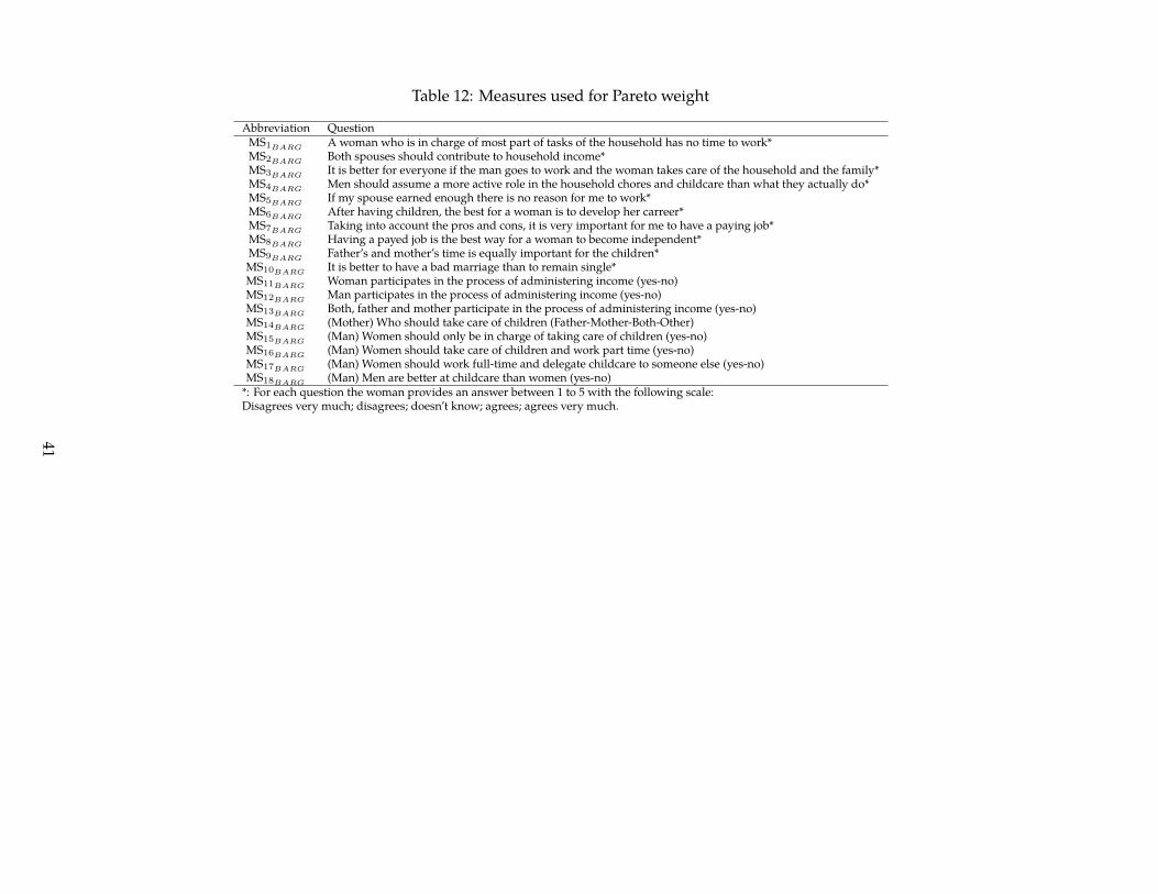
Table 12: Measures used for Pareto weight

Abbreviation QuestionMS1BARG A woman who is in charge of most part of tasks of the household has no time to work*MS2BARG Both spouses should contribute to household income*MS3BARG It is better for everyone if the man goes to work and the woman takes care of the household and the family*MS4BARG Men should assume a more active role in the household chores and childcare than what they actually do*MS5BARG If my spouse earned enough there is no reason for me to work*MS6BARG After having children, the best for a woman is to develop her carreer*MS7BARG Taking into account the pros and cons, it is very important for me to have a paying job*MS8BARG Having a payed job is the best way for a woman to become independent*MS9BARG Father’s and mother’s time is equally important for the children*MS10BARG It is better to have a bad marriage than to remain single*MS11BARG Woman participates in the process of administering income (yes-no)MS12BARG Man participates in the process of administering income (yes-no)MS13BARG Both, father and mother participate in the process of administering income (yes-no)MS14BARG (Mother) Who should take care of children (Father-Mother-Both-Other)MS15BARG (Man) Women should only be in charge of taking care of children (yes-no)MS16BARG (Man) Women should take care of children and work part time (yes-no)MS17BARG (Man) Women should work full-time and delegate childcare to someone else (yes-no)MS18BARG (Man) Men are better at childcare than women (yes-no)

*: For each question the woman provides an answer between 1 to 5 with the following scale:Disagrees very much; disagrees; doesn’t know; agrees; agrees very much.

41

Table 13: Father’s opinion on gender roles

Item Number Per centWomen should only spend time taking care of chidlren 3,925 34.34Women should take care of children and work if there is remaining time 6,930 60.62Women should work full time 525 4.59Men take care better of children than women 51 0.45Total 11,431 100.00

Table 14: Summary statistics-Measures of bargaining power

Variable Mean (Std. Dev.)A woman in charge of chores should not work 2.59 (1.03)Both parents should contribute equally to household income 1.85 (0.95)It is better if the man goes to work and the woman stays at home 2.57 (1.06)Men should be more involved in household chores 1.84 (0.99)If husband earned enough there is no reason for woman to work 2.55 (1.6)It is better if woman has children after having a succesful carreer 2.45 (1.25)It is very important for a woman to have a job 1.94 (1.06)Having a job is the best way for a woman to achieve independence 1.86 (0.98)Father’s time is as important as mother’s time for children 1.56 (0.87)It is better to have a bad marriage than being single 3.57 (1.4)

N 15754

All questions are answered by the mother of the child. The possible answers are 1: strongly agrees; 2: agrees; 3: disagrees;

4: strongly disagrees.

Table 15: Summary statistics-Variables determining Pareto weight

Variable Mean (Std. Dev.) NFather’s non-labor income share 0.27 (0.34) 4470Age difference (Father-Mother) 3.01 (5.18) 4470Difference in grades attained (Father-Mother) -0.21 (2.82) 4470Sex ratio in region (Women/Men) 1.01 (0.06) 4470Unemployment ratio in region (Men/Women) 0.67 (0.11) 4470Wage ratio in region (Men/Women) 1.41 (0.07) 4470Distance to women protection center (km) 19.15 (31.79) 4465

The ratio of wages offered is not reported in these table as is the results of the parameters estimated in the model. The share of father’s

non-labor income, as well as the age difference and the differences in grades attained are all obtained from the ECLS dataset. The sex ratio

in the city is computed using information from the CENSUS dataset. The last CENSUS available for Chile is from 2002. I use information

about female-male ratio based on the population projections from the National Institute of Statistics fro Chile. The unemployment and wage

information is obtained from the CASEN household survey of 2011.

42

Table 16: Time investments and labor supply (2010)

(1) (2)VARIABLES Mother’s effort (2010) Father’s effort (2010)

Mother: hours worked weekly -0.00*** 0.00***(0.00) (0.00)

Father: hours worked weekly 0.00*** -0.00***(0.00) (0.00)

Total household income 0.00 0.00***(0.00) (0.00)

Age of child (months) 0.01*** 0.00*(0.00) (0.00)

BFI-Extraversion 0.05*** 0.07***(0.02) (0.02)

BFI-Kindness 0.05** 0.04*(0.02) (0.02)

BFI-Responsibility 0.06*** 0.05**(0.02) (0.02)

BFI-Neuroticism -0.05*** -0.02(0.01) (0.02)

BFI-Openness 0.15*** 0.02(0.02) (0.02)

Wais-digits 0.01 0.01*(0.01) (0.01)

Wais-Vocabulary -0.00 -0.00(0.00) (0.00)

Number of siblings -0.07*** -0.06***(0.01) (0.01)

Observations 7,058 7,058Adjusted R-squared 0.07 0.04

Robust standard errors in parentheses*** p<0.01, ** p<0.05, * p<0.1

Additional controls include age of child, race, age of both parents and test scores of primary caregiver.

The measure of effort is constructed via Principal component analysis, extracting one factor for the variables used asmeasures of time investments by parents. The measures of parental effort, together with the big five personality test scoresand the Wais cognitive assessments are all standardized to have mean zero and one standard deviation. In the regression themeasure of effort is in hundreds.

43

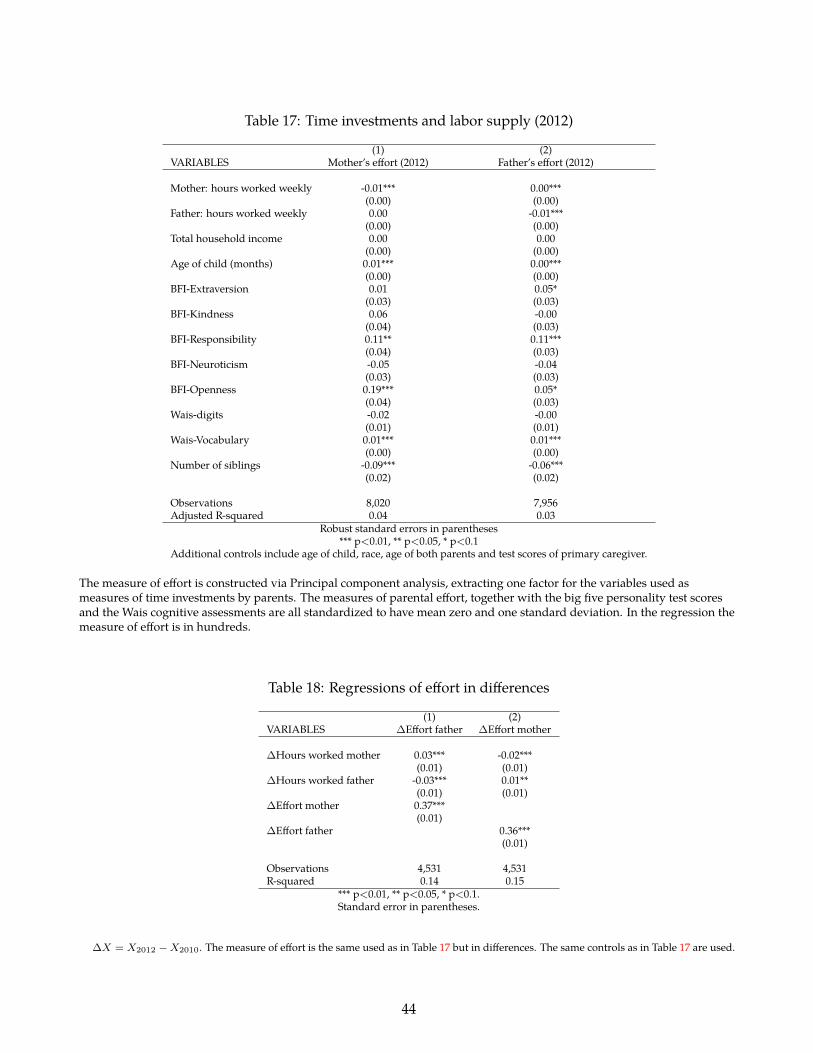
Table 17: Time investments and labor supply (2012)

(1) (2)VARIABLES Mother’s effort (2012) Father’s effort (2012)

Mother: hours worked weekly -0.01*** 0.00***(0.00) (0.00)

Father: hours worked weekly 0.00 -0.01***(0.00) (0.00)

Total household income 0.00 0.00(0.00) (0.00)

Age of child (months) 0.01*** 0.00***(0.00) (0.00)

BFI-Extraversion 0.01 0.05*(0.03) (0.03)

BFI-Kindness 0.06 -0.00(0.04) (0.03)

BFI-Responsibility 0.11** 0.11***(0.04) (0.03)

BFI-Neuroticism -0.05 -0.04(0.03) (0.03)

BFI-Openness 0.19*** 0.05*(0.04) (0.03)

Wais-digits -0.02 -0.00(0.01) (0.01)

Wais-Vocabulary 0.01*** 0.01***(0.00) (0.00)

Number of siblings -0.09*** -0.06***(0.02) (0.02)

Observations 8,020 7,956Adjusted R-squared 0.04 0.03

Robust standard errors in parentheses*** p<0.01, ** p<0.05, * p<0.1

Additional controls include age of child, race, age of both parents and test scores of primary caregiver.

The measure of effort is constructed via Principal component analysis, extracting one factor for the variables used asmeasures of time investments by parents. The measures of parental effort, together with the big five personality test scoresand the Wais cognitive assessments are all standardized to have mean zero and one standard deviation. In the regression themeasure of effort is in hundreds.

Table 18: Regressions of effort in differences

(1) (2)VARIABLES ∆Effort father ∆Effort mother

∆Hours worked mother 0.03*** -0.02***(0.01) (0.01)

∆Hours worked father -0.03*** 0.01**(0.01) (0.01)

∆Effort mother 0.37***(0.01)

∆Effort father 0.36***(0.01)

Observations 4,531 4,531R-squared 0.14 0.15

*** p<0.01, ** p<0.05, * p<0.1.Standard error in parentheses.

∆X = X2012 −X2010. The measure of effort is the same used as in Table 17 but in differences. The same controls as in Table 17 are used.

44

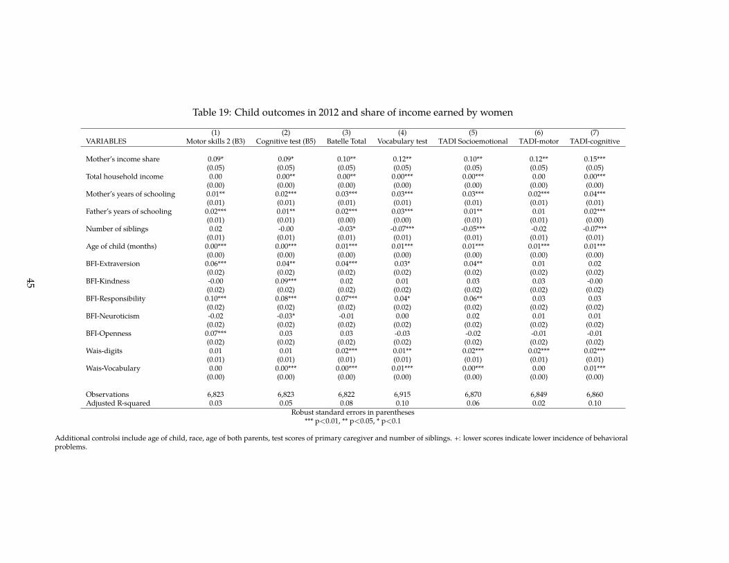
Table 19: Child outcomes in 2012 and share of income earned by women

(1) (2) (3) (4) (5) (6) (7)VARIABLES Motor skills 2 (B3) Cognitive test (B5) Batelle Total Vocabulary test TADI Socioemotional TADI-motor TADI-cognitive

Mother’s income share 0.09* 0.09* 0.10** 0.12** 0.10** 0.12** 0.15***(0.05) (0.05) (0.05) (0.05) (0.05) (0.05) (0.05)

Total household income 0.00 0.00** 0.00** 0.00*** 0.00*** 0.00 0.00***(0.00) (0.00) (0.00) (0.00) (0.00) (0.00) (0.00)

Mother’s years of schooling 0.01** 0.02*** 0.03*** 0.03*** 0.03*** 0.02*** 0.04***(0.01) (0.01) (0.01) (0.01) (0.01) (0.01) (0.01)

Father’s years of schooling 0.02*** 0.01** 0.02*** 0.03*** 0.01** 0.01 0.02***(0.01) (0.01) (0.00) (0.00) (0.01) (0.01) (0.00)

Number of siblings 0.02 -0.00 -0.03* -0.07*** -0.05*** -0.02 -0.07***(0.01) (0.01) (0.01) (0.01) (0.01) (0.01) (0.01)

Age of child (months) 0.00*** 0.00*** 0.01*** 0.01*** 0.01*** 0.01*** 0.01***(0.00) (0.00) (0.00) (0.00) (0.00) (0.00) (0.00)

BFI-Extraversion 0.06*** 0.04** 0.04*** 0.03* 0.04** 0.01 0.02(0.02) (0.02) (0.02) (0.02) (0.02) (0.02) (0.02)

BFI-Kindness -0.00 0.09*** 0.02 0.01 0.03 0.03 -0.00(0.02) (0.02) (0.02) (0.02) (0.02) (0.02) (0.02)

BFI-Responsibility 0.10*** 0.08*** 0.07*** 0.04* 0.06** 0.03 0.03(0.02) (0.02) (0.02) (0.02) (0.02) (0.02) (0.02)

BFI-Neuroticism -0.02 -0.03* -0.01 0.00 0.02 0.01 0.01(0.02) (0.02) (0.02) (0.02) (0.02) (0.02) (0.02)

BFI-Openness 0.07*** 0.03 0.03 -0.03 -0.02 -0.01 -0.01(0.02) (0.02) (0.02) (0.02) (0.02) (0.02) (0.02)

Wais-digits 0.01 0.01 0.02*** 0.01** 0.02*** 0.02*** 0.02***(0.01) (0.01) (0.01) (0.01) (0.01) (0.01) (0.01)

Wais-Vocabulary 0.00 0.00*** 0.00*** 0.01*** 0.00*** 0.00 0.01***(0.00) (0.00) (0.00) (0.00) (0.00) (0.00) (0.00)

Observations 6,823 6,823 6,822 6,915 6,870 6,849 6,860Adjusted R-squared 0.03 0.05 0.08 0.10 0.06 0.02 0.10

Robust standard errors in parentheses*** p<0.01, ** p<0.05, * p<0.1

Additional controlsi include age of child, race, age of both parents, test scores of primary caregiver and number of siblings. +: lower scores indicate lower incidence of behavioralproblems.

45

Table 20: Female empowerment and Child outcomes

(1) (2) (3) (4) (5)VARIABLES Toys for development Fruits and vegetables Bread Cookies and candies People sharing bedroom with child

Total household income 0.00*** 0.00 -0.00* 0.00 -0.00***(0.00) (0.00) (0.00) (0.00) (0.00)

Mother’s years of schooling 0.01*** 0.01** -0.01 0.01* -0.03***(0.00) (0.01) (0.01) (0.01) (0.00)

Father’s years of schooling 0.01*** 0.01** -0.00 -0.00 -0.02***(0.00) (0.00) (0.00) (0.01) (0.00)

Number of siblings 0.00 0.04** 0.01 0.00 0.08***(0.01) (0.01) (0.01) (0.02) (0.01)

People in household -0.01** 0.01 0.01 0.02* 0.13***(0.01) (0.01) (0.01) (0.01) (0.01)

Woman administers+ 0.03** 0.09*** -0.04* 0.08*** -0.00(0.01) (0.02) (0.02) (0.03) (0.02)

Gender roles -Woman++ -0.01 -0.03** 0.02 -0.02 0.02*(0.01) (0.01) (0.01) (0.02) (0.01)

Gender roles - Man++ -0.01 -0.05* -0.04 -0.02 0.06**(0.01) (0.03) (0.03) (0.03) (0.02)

Observations 6,344 8,245 8,242 8,241 8,246Adjusted R-squared 0.04 0.03 0.02 0.01 0.19

Robust standard errors in parentheses*** p<0.01, ** p<0.05, * p<0.1

Consumption of bread, fruits and vegetables and cookies and candies is related to the frequency of consumption of this food on a weekly basis. More details can be found in Table 11. +dummy variable indicating whether the mother is the person in charge of administering the resources of the household (1) or no (0). ++ opinion of gender roles according to the manand the woman. A value of one indicates that the person agrees with the sentence ”Women should not work and should only take care of children”.

46

Table 21: Description of sample used in the analysis

Filter Number of householdsInitial sample 18,310Household not surveyed in 2012 16,033Household not surveyed in 2010 12,898Parent not living in household 7,855Siblings within five years of age in the household 4,125Children with incomplete skills questionnaires 2,247Households with incomplete questionnaires 950

Table 22: Descriptive statistics - Families in 2012

Variable Mean 25% 75% SdMother’s age 34.52 29.00 39.00 6.94Father’s age 37.41 32.00 43.00 7.96Mother’s years of schooling 11.27 10.00 12.00 2.97Father’s years of schooling 10.72 8.00 12.00 3.13Mother’s hours of work (week) 24.22 0.00 45.00 21.34Father’s hours of work (week) 43.20 45.00 48.00 16.03Mother’s weekly wage (1,000 CLP) 82.73 41.86 95.24 92.78Mother’s weekly wage (USD) 165.46 83.72 190.49 185.55Father’s weekly wage (1,000 CLP) 85.48 42.62 93.02 88.19Father’s weekly wage (USD) 170.95 85.23 186.05 176.39Household’s total Income (Weekly-CLP) 124.55 59.88 151.16 108.83Household’s total Income (Weekly (USD)) 249.10 119.76 302.33 217.66Age of child (months) 64.60 58.00 72.00 8.40

All summary statistics are reported for the survey used in 2012.

Table 23: Age distribution (2012)

Item Number Per cent4 310 32.635 397 41.796 243 25.58

Total 950 100.00

47

Table 24: Estimates: Utility function. Mother’spreferences

Parameter Estimate Standard Errorαm1,12 0.6312 0.0028αm2,12 0.0517 0.0001αm3,12 0.3035 0.2208αm4,0,12 0.0136 0.0001αm4,1,12 0.0012 0.0001αm1,10 0.0554 0.0003αm2,10 0.0038 0.0001αm3,10 0.1026 0.2437αm4,0,10 0.0001 0.0001αm4,1,10 0.0001 0.0001αm5,10 0.8381 0.3831

Table 25: Estimates: Utility function. Father’spreferences

Parameter Estimate Standard Errorαf1,12 0.1587 0.0026αf2,12 0.0339 0.0001αf3,12 0.8042 0.3610αf4,0,12 0.0032 0.0001αf4,1,12 0.0016 0.0001αf1,10 0.6157 0.0026αf2,10 0.1407 0.0005αf3,10 0.8042 0.4496αf4,0,10 0.0114 0.0001αf4,1,10 0.0001 0.0001αf5,10 0.0057 1.0415

Table 26: Estimates: Preference shock

Parameter Estimate Standard ErrorσmW,A 3.6627 0.8352σmNW,A 0.9095 0.1140σmNW,NA 0.0794 0.2469σfW,A 0.5020 0.4519σfNW,A 0.0851 0.4550σfNW,NA 0.0020 0.0777Preference shocks for work-no childcare are standardized to zero

Table 27: Estimates: Mothers wages

Parameter Estimate Standard Errorβm0 5.7874 0.4394βm1 0.2757 0.0251βm2 0.0732 0.0379βm3 -0.0006 0.0006σwm 0.8280 0.0606

Table 28: Estimates: Fathers wages

Parameter Estimate Standard Errorβf0 5.8103 0.2997βf1 0.1260 0.0055βf2 0.1875 0.0156βf3 -0.0022 0.0002σwf 0.6894 0.0130

48

Table 29: Estimates: Production of Skills

Parameter Estimate Standard Errorθ0 0.2128 0.0011θ1 0.2673 0.0017θ2 0.5199 0.0032φ 0.4688 0.0007γf 0.3647 0.0006γm 0.6353 0.0016δ0 -0.8000 0.0051δ1 -0.0000 0.0001δ2 0.0010 0.0004δ3,10 3.5038 0.0172δ3,12 5.3000 0.0408δ4 0.0130 0.0001σs 1.5754 0.0065

Table 30: Estimates: Distribution of latent fac-tors

Parameter Estimate Standard Errorσmef 2.5133 0.0039σfef 3.3754 0.0025σinv 2.1896 0.0144

Table 31: Estimates: Prices

Parameter Estimate Standard ErrorPriceI0 966.2378 1.8225PriceI1 1.0537 0.0019

Pchildcare0 2440.6020 1.1684Pchildcare1 622.6098 1.2417

Table 32: Estimates: Pareto weight

Parameter Estimate Standard Error Descriptionλ0 -2.7321 0.0136 Interceptλ1 0.0023 0.0143 Wage ratioλ2 0.0527 0.0006 Non-labor income ratioλ3 -0.1194 0.0001 Age differenceλ4 0.0036 0.0026 Educational differenceλ5 -2.5325 0.0039 Gender ratioλ6 -0.0069 0.0328 Unemployment ratioλ7 -0.7722 0.0006 Wage ratio (region)σµ 0.5179 0.0074 Standard deviation

Table 33: Model Fit - I

Female Labor Force Participation Predicted Data2010 57.2% 60.28%2012 62.6% 61.47%

Table 34: Model Fit - II

Male Labor Force Participation Predicted Data2010 91.8% 94.6%2012 96.1% 93.2%

Table 35: Model Fit - III

Childcare Attendance Predicted DataWorking Mothers 68.4% 67.7%Not-working Mothers 41.6% 42.9%

Table 36: Effects of Policy counterfactuals. Change in Female employment (percentage points)

Counterfactual Effect on Female employment1 -0.632 -0.633 0.634 0.00

49

Table 37: Effects of Policy counterfactuals. Change in Male employment (percentage points)

Counterfactual Effect on Male employment1 -0.212 -0.213 0.004 0.00

Table 38: Effects of Policy counterfactuals. Change in Money invested

Counterfactual Change in Money Invested1 11.362 11.363 34.084 333.59

Table 39: Effects of Policy counterfactuals. Change in Money invested

Counterfactual Change in Money Invested1 11.362 11.363 34.084 333.59

Table 40: Cost of policy interventions

Counterfactual Expenditure per capita (USD)Transfers to Mother 449.59Transfers to Father 449.59Childcare Subsidy* 221.64In-kind transfers 449.59

Figure 1: Information on Preschool Providers

0

1000

2000

3000

4000

5000

0 100 200 300 400Number of institutions. Mean=109.61

Num

ber

of h

ouse

hold

s

Preschool institutions within 5km

0

500

1000

1500

2000

0 1 2 3Distance (km). Mean=0.61km

Num

ber

of h

ouse

hold

s

Distance to nearest preschool institution

50

Figure 2: Example of distribution of childcare providers. City of “La Serena”, Chile

51

Figure 3: Weekly frequency of activities between parents and children

For each activity there are possible answers: 0: never, 1: one to three times a week; 2: four to six times a week; 3: everyday.

52

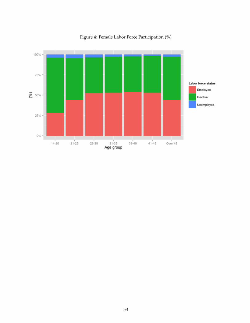
Figure 4: Female Labor Force Participation (%)

53

Figure 5: Gaps in health at birth (%)

4546474849505152535455

cm

1 2 3 4 5Income quintile

Height at birth

3

3.5

4Kg

1 2 3 4 5Income quintile

Weight at birth

123456789

10

%

1 2 3 4 5Income quintile

Pre-term births

54

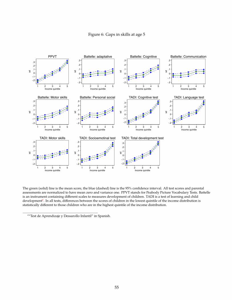
Figure 6: Gaps in skills at age 5

-.2-.1

0.1.2.3

sd

1 2 3 4 5Income quintile

PPVT

-.2

-.1

0

.1

.2

.3

sd

1 2 3 4 5Income quintile

Battelle: adaptative

-.2

-.1

0

.1

.2

.3

sd

1 2 3 4 5Income quintile

Battelle: Cognitive

-.2

-.1

0

.1

.2

.3

sd

1 2 3 4 5Income quintile

Battelle: Communication

-.2

-.1

0

.1

.2

.3

sd

1 2 3 4 5Income quintile

Battelle: Motor skills

-.2

-.1

0

.1

.2

.3

sd

1 2 3 4 5Income quintile

Battelle: Personal social

-.2-.1

0.1.2.3

sd

1 2 3 4 5Income quintile

TADI: Cognitive test

-.2

-.1

0

.1

.2

.3

sd

1 2 3 4 5Income quintile

TADI: Language test

-.2

-.1

0

.1

.2

.3

sd

1 2 3 4 5Income quintile

TADI: Motor skills

-.2

-.1

0

.1

.2

.3

sd

1 2 3 4 5Income quintile

TADI: Socioemotinal test

-.2-.1

0.1.2

.3

sd

1 2 3 4 5Income quintile

TADI: Total development test

The green (solid) line is the mean score, the blue (dashed) line is the 95% confidence interval. All test scores and parentalassessments are normalized to have mean zero and variance one. PPVT stands for Peabody Picture Vocabulary Tests. Battelleis an instrument containing different scales to measures development of children. TADI is a test of learning and childdevelopmenta. In all tests, differences between the scores of children in the lowest quintile of the income distribution isstatistically different to those children who are in the highest quintile of the income distribution.

a“Test de Aprendizaje y Dessarollo Infantil” in Spanish.

55

Figure 7: Monetary Transfers to Families in Chile

The graph reports the relationship between monetary transfers that families receive from the central government, on amonthly basis, from three main programs: “Unique Family Subsidies”a, “Family Assignments”b and “Social ProtectionTransfer”c and their score in the Social Protection Cardd. The conditions to be eligible for these programs are to have a score inthe Social Protection Card below 11.734 and for those who work, having a monthly income of less than $187,515 CLP. Thefinal amount being transferred to the household also depends on the size of the household and the time they have beenbeneficiaries of such programs. The solid line represents the schedule for a family composed of two adults and one child whohas been in the program for 50 months. The dashed line corresponds to a bi-parental household with three children under 18who have been in the program for less than six months.

a“Asignacion Unica Familia” in Spanish.b‘Asignacion Familiar” in Spanishc“Bono de proteccion social”d“Ficha de Proteccion Social”

56

Figure 8: Model fit: Female labor force participation according to education

0.00

0.25

0.50

0.75

1.00

5 10 15 20Years of schooling

Pro

port

ion

wor

king

ObservedPredicted

2010

0.00

0.25

0.50

0.75

1.00

5 10 15 20Years of schooling

Pro

port

ion

wor

king

ObservedPredicted

2012

Figure 9: Model fit: Male labor force participation according to education

0.00

0.25

0.50

0.75

1.00

5 10 15 20Years of schooling

Pro

port

ion

wor

king

ObservedPredicted

2010

0.00

0.25

0.50

0.75

1.00

5 10 15 20Years of schooling

Pro

port

ion

wor

king

ObservedPredicted

2012

57

Figure 10: Bootstrap fit: Parents’ Labor Force Participation in 2012

0.00

0.25

0.50

0.75

1.00

5 10 15 20Years of schooling

Pro

port

ion

wor

king

Women−2012

0.00

0.25

0.50

0.75

1.00

5 10 15 20Years of schooling

Pro

port

ion

wor

king

Men−2012

Dashed lines represent the 95% confidence interval

Figure 11: Bootstrap fit: Childcare decisions (%)

0.00

0.25

0.50

0.75

1.00

Not−working WorkingWork status

Pro

port

ion

atte

ndin

g

Observed

Predicted

Childcare attendance

Brackets include the 95% confidence interval

58

Figure 12: Model fit: distribution of wages

Kernel density estimates of predicted and observed wages. Bandwidth chosen is 3.

59

Figure 13: Distribution of skills. Smoothing distribution

−0.6

−0.3

0.0

0.3

0.6

0 25 50 75 100Percentile (Income)

Ski

lls−

Sta

ndar

d D

evia

tions

Mean 95% Confidence Interval

60

Figure 14: Signal to noise ratio. Mother’s effort (2012)

MS14

MS13

MS11

MS10

MS6

MS7

MS3

MS8

MS12

MS1

MS9

MS2

MS4

MS5

0 25 50 75 100Signal to noise (%)

61

Figure 15: Signal to noise ratio. Monetary Investment (2012)

MS15

MS16

MS13

MS19

MS12

MS18

MS14

MS17

MS20

MS21

MS6

MS8

MS11

MS5

MS4

MS10

MS2

MS9

MS1

MS3

MS7

0 25 50 75 100Signal to noise (%)

62

Figure 16: Effects of Policy Interventions

Effects on the gap in skills between the top 20% richest households and the poorest 20% of thehouseholds

−8

−6

−4

−2

0

Cas

h tr

ansf

er to

Fat

her

Cas

h tr

ansf

er to

Mot

her

Chi

ldca

re S

ubsi

dy

In−

kind

Tra

nsfe

r

% C

hang

e in

20−

20 g

ap

Cash transfer to Father

Cash transfer to Mother

Childcare Subsidy

In−kind Transfer

63

Figure 17: Effects of Policy Interventions

Effects on the gap in skills between the top 20% richest households and the poorest 20% of thehouseholds when money spent in each policy is the same.

−4

−2

0%

Cha

nge

in 2

0−20

gap

in s

kills

(pe

rcen

tage

poi

nts)

Cash transfer to FatherCash transfer to MotherChildcare SubsidyIn−kind Transfer

64

References

Attanasio, O. P., & Lechene, V. (2014). Efficient responses to targeted cash transfers. Journal of PoliticalEconomy, 122(1), 178–222.

Basu, K. (2006). Gender and say: a model of household behaviour with endogenously determinedbalance of power*. The Economic Journal, 116(511), 558–580.

Bernal, R. (2008). The effect of maternal employment and child care on children’s cognitive development.International Economic Review, 49(4), 1173–1209.

Blundell, R., Chiappori, P.-A., & Meghir, C. (2005). Collective labor supply with children. Journal ofpolitical Economy, 113(6), 1277–1306.

Bobonis, G. J. (2009). Is the allocation of resources within the household efficient? new evidence from arandomized experiment. Journal of political Economy, 117(3), 453–503.

Borghans, L., Duckworth, A. L., Heckman, J. J., & Ter Weel, B. (2008). The economics and psychology ofpersonality traits. Journal of human Resources, 43(4), 972–1059.

Browning, M., Chiappori, P.-A., & Lewbel, A. (2013). Estimating consumption economies of scale, adultequivalence scales, and household bargaining power. The Review of Economic Studies, rdt019.

Browning, M., Chiappori, P.-A., & Weiss, Y. (2014). Economics of the family. Cambridge University Press.Bruins, M. (2015). Taxes, welfare and the resources parents allocate to children. Unpublished manuscript.Carneiro, P., Hansen, K., & Heckman, J. (2003). Estimating distributions of treatment effects with an

application to the returns to schooling and measurement of the effects of uncertainty on collegechoice. International Economic Review, 44(2), 361-422.

Cesarini, D., Lindqvist, E., Notowidigdo, M. J., & Ostling, R. (2013). The effect of wealth on household laborsupply: Evidence from swedish lotteries.

Cherchye, L., De Rock, B., & Vermeulen, F. (2012). Married with children: A collective labor supplymodel with detailed time use and intrahousehold expenditure information. The American EconomicReview, 102(7), 3377–3405.

Chiappori, P.-A., & Donni, O. (2009). Non-unitary models of household behavior: A survey of the literature(Tech. Rep.). IZA Discussion Papers.

Chile, G. o. (2013). Chile en el panorama educacional internacional.Chile, U. (2010). “primera ronda de la encuesta longitudinal de la primera infancia” [Computer software

manual].Conti, G., & Heckman, J. J. (2012). The economics of child well-being. NBER Working Paper, 18466.Creal, D. (2012). A survey of sequential monte carlo methods for economics and finance. Econometric

Reviews, 31(3), 245–296.Cunha, F., & Heckman, J. J. (2008). Formulating, identifying and estimating the technology of cognitive

and noncognitive skill formation. Journal of Human Resources, 43(4), 738–782.Cunha, F., Heckman, J. J., & Schennach, S. M. (2010). Estimating the technology of cognitive and noncog-

nitive skill formation. Econometrica, 78(3), 883–931.Del Boca, D., Flinn, C., & Wiswall, M. (2014). Household choices and child development. The Review of

Economic Studies, 81(1), 137–185.

65

Del Boca, D., Flinn, C. J., & Wiswall, M. (2016). Transfers to households with children and child devel-opment. Economic Journal, Forthcoming.

Doepke, M., & Tertilt, M. (2014). Does female empowerment promote economic development? (Tech. Rep.).National Bureau of Economic Research.

Duflo, E. (2000). Grandmothers and grandaughters: the effects of old age pension on child health insouth africa.

Duncan, G. J., & Magnuson, K. (2013). Investing in preschool programs. The Journal of Economic Perspec-tives, 27(2), 109–132.

Fiorini, M., & Keane, M. P. (2014). How the allocation of children’s time affects cognitive and noncognitivedevelopment. Journal of Labor Economics, 32(4), 787–836.

Fiszbein, A., Schady, N. R., & Ferreira, F. H. (2009). Conditional cash transfers: reducing present and futurepoverty. World Bank Publications.

Francesconi, M., & Heckman, J. (2016). Symposium on child development and parental investment:Introduction. IZA DP, 9977.

Gayle, G.-L., Golan, L., & Soytas, M. A. (2015). What accounts for the racial gap in time allocation andintergenerational transmission of human capital?

Haddad, L., Hoddinott, J., Alderman, H., et al. (1997). Intrahousehold resource allocation in developingcountries: models, methods, and policy. Johns Hopkins University Press.

Heckman, J., & Mosso, S. (2014). The economics of human development and social mobility. AnnualReview of Economics, 6, 689-733.

Heckman, J. J., Stixrud, J., & Urzua, S. (2006). The effects of cognitive and noncognitive abilities on labormarket outcomes and social behavior. Journal of Labor Economics, 24(3), 411-482.

Keane, M., Todd, P., & Wolpin, K. (2011). The structural estimation of behavioral models: Discrete choicedynamic programming methods and applications. Handbook of Labor Economics, 4a(331-461).

Klaas, M., Briers, M., De Freitas, N., Doucet, A., Maskell, S., & Lang, D. (2006). Fast particle smoothing:If i had a million particles. In Proceedings of the 23rd international conference on machine learning (pp.481–488).

Macours, K., Schady, N., & Vakis, R. (2012). Cash transfers, behavioral changes, and cognitive devel-opment in early childhood: evidence from a randomized experiment. American Economic Journal:Applied Economics, 4(2), 247–273.

Matzkin, R. L. (2007). Nonparametric identification. Handbook of Econometrics, 6, 5307–5368.Murphy, K. P. (2012). Machine learning: a probabilistic perspective. MIT press.Nelson, C. A., & Sheridan, M. A. (2011). Lessons from neuroscience research for understanding causal

links between family and neighborhood characteristics and educational outcomes. Whither oppor-tunity, 27–46.

Paxson, C., & Schady, N. (2010). Does money matter? the effects of cash transfers on child developmentin rural ecuador. Economic development and cultural change, 59(1), 187–229.

Roberts, B. W., Kuncel, N. R., Shiner, R., Caspi, A., & Goldberg, L. R. (2007). The power of personality: Thecomparative validity of personality traits, socioeconomic status, and cognitive ability for predicting

66

important life outcomes. Perspectives on Psychological Science, 2(4), 313–345.Schady, N., Behrman, J., Araujo, M. C., Azuero, R., Bernal, R., Bravo, D., . . . others (2015). Wealth

gradients in early childhood cognitive development in five Latin American countries. Journal ofHuman Resources, 50(2), 446–463.

Schennach, S. (2004). Estimation of nonlinear models with measurement error. Econometrica, 72(1),33-75.

Schoellman, T. (2014). Early childhood human capital and development. American Economic Journal:Macroeconomics.

Sørensen, H. T., Sabroe, S., Rothman, K. J., Gillman, M., Steffensen, F. H., Fischer, P., & Serensen, T. I.(1999). Birth weight and length as predictors for adult height. American Journal of Epidemiology,149(8), 726–729.

Thomas, D. (1994). Like father, like son; like mother, like daughter: Parental resources and child height.Journal of human resources, 950–988.

Thomas, D., Contreras, D., & Frankenberg, E. (2002). Distribution of power within the household andchild health. Santa Monica: RAND. Mimeo.

Todd, P. E., & Wolpin, K. I. (2007). The production of cognitive achievement in children: Home, school,and racial test score gaps. Journal of Human capital, 1(1), 91–136.

67

10 Appendix

10.1 Identification of Measurement System

The measurement system is described by:

Z = ι0 + ι1K + ε (60)

We normalize E[k] = 0 for every factor. The variance-covariance matrix of the measurement system isgiven by:

ΣZ = ι1ΣKι′1 + Σε (61)

The matrix of moments ΣZ containsM(M+1)/2 moments in order to identify the necessary parametersof the models. M is the total number of measures available and is equal to the sum of measures for eachfactor:

M =∑k∈K

Nk = 151 (62)

as we have

Nln(S0) = 23

Nln(S1) = 11

Nln(S2) = 13

Nln(PG) = 8

Nµ = 19

Nln(I1) = 8

Nln(I2) = 21

Nln(ef1 )

= 10

Nln(ef2 )

= 14

Nln(em1 ) = 10

Nln(em2 ) = 14

The dedicated factor structure assumed imposes that each measure loads exclusively to one factor.This implies that rather than 11 ×M factor loadings to obtain we only have to estimate M elements inι1 to be estimated. Given that the scale of the factor is irrelevant for the analysis, we can normalize onefactor loading for each factor to be 1. In total, we have M − 11 = 140 factor loadings to be estimated.

The matrix ΣK contains (11 × (11 + 1)/2) covariances to be estimated and Σε has M × (M + 1)/2.We see that it is necessary to make some assumptions about the correlation structure of the factors or

68

of the measurement error system in order to be able to identify the system. If we assume that the mea-surement error in the system for skills at birth is independent of measurement error in the remainingsystems εln(s0)

m ⊥⊥ ε′km for m = 1...Nln(s0), k ∈ K, k 6= ln(s0), m′ = 1...Nk we have enough moments toidentify the system. By doing this assumption, we are assuming that the elements in Σε that correspondcorresponding to ln(s0) and other factors are zero. With this, we have enough moments to identify thesystem.

69

10.2 Estimation

In this section I will derive the full likelihood function of the model as well as the filtering procedure toestimate it.

10.2.1 Likelihood function

The likelihood of the model is:

L (Θ|O;X) = P (O|X; Θ) = P (O1, O2, O3|X; Θ)

p0(O0|Θ, X)p1(O1|O0,Θ, X)p2(O2|O1,Θ, X) (63)

Now, inspecting every element. The first term is composed by the observed outcomes in period zero.Given that the only one observed in this case is the first period of skills, this is composed then by that.

p0(O0|Θ, X) =

∫p0(O0,K0|Θ, X)dK0 =

∫p0(O0|K0,Θ, X)p(K0|Θ, X)dK0 =

Ep(K0|Θ,X) [P0(O0|K0,Θ, X)] ≈

RR∑rr=1

P0(O0|Krr0 ,Θ, X) (64)

for RR large, and for the Krr0 RRrr=1 being drawn from the distribution p(K0|Θ, X). K0 is the set ofunobserved factors relevant for period zero given by

K0 = ln(s0), ln(PG) (65)

Note that in the model the distribution p(K0|Θ, X) is not specified. I will assume that both factors areindependent and each follow a normal distribution with mean zero and variance σ2

s0 and σ2PG respec-

tively. This way, evaluating the likelihood for period 0 ends up being a process of drawing shocks fromthe distribution p(K0|Θ, X), computing the likelihood of each shock given by the measurement systemof the unobserved latent factors and averaging such likelihoods over the RR shocks.

For the first period the set of relevant factors is given by:

K1 = ln(s1), ln(ef,∗1 ), ln(em,∗1 ), ln(I∗1 ), µ1 (66)

and the likelihood can be expressed as:

70

p1(O1|O0,Θ, X) =

∫p1(O1,K1|O0,Θ, X)dK1 =

∫ ∫p1(O1,K1,K0|O0,Θ, X)dK1dK0 =

∫ ∫p1(O1|K1,K0, O0,Θ, X)p(K1|O0,K0,Θ, X)p(K0|O0,Θ, X)dK1dK0 (67)

Note that

p(K1|O0,K0,Θ, X) = p(K1|K0, θ,X) (68)

as O0 would not carry more information beyond that in K0 that is relevant for K1. Also, note that

p1(O1|K1,K0, O0,Θ, X) = p1(O1|K1,Θ, X) (69)

Taking into account the facts presented in Equations 68 and 69 we can express 67 as:∫ ∫p1(O1|K1,Θ, X)p(K1|K0,Θ, X)p(K0|O0,Θ, X)dK1dK0 =

∫p(K0|O0,Θ, X)

[∫p(O1|K1,Θ, X)p(K1|K0,Θ, X)dK1

]dK0 =

Ep(K0|O0,Θ,X)

[∫p(O1|K1,Θ, X)p(K1|K0,Θ, X)dK1

]= (70)

in Equation 70 p(O1|K1,Θ, X) is given by the measurement system of factors, the likelihood of wages(for those that are observed) and the preference shocks cdf. We can re-write such expression as:

p(O1|K1,Θ, X) =

p(Z1|K1,Θ, X)× p(wf |K1,Θ, X)(1−hf,∗) × p(wm|K1,Θ, X)1−hm,∗

× p(hf,∗, hm,∗, a|wf , wm,K1,Θ, X) (71)

As specified previously, p(Z1|K1,Θ, X) is given by the measurement system. p(wf |K1,Θ, X) is given bythe measurement error associated to the observed wages:

ln(wj)

= βj0 + βj1yrschoolj + βj2Age

j + βj3(Agej)2 + εwj (72)

71

where εwj is measurement error following a distribution εwj ∼ N(0, σεj ).Finally, p(h∗f , h∗m, a∗|wf , wm,K1,Θ, X) is given by the probability of having the observed decisions as theoptimal ones:

p(h∗f , h∗m, a

∗|wf , wm,K1,Θ, X) =

p(εfd,ε

md )

(W (uf (hf∗, hm,∗, a∗), um(hf,∗, hm,∗, a∗)) ∈ arg max

hf ,hm,aW (uf (hf , hm, a), um(hf , hm, a))|K1,Θ, X

)(73)

where p(εfd,ε

md )

is the distribution of the preference shocks εfd , εmd .

p(K1|K0,Θ, X) is given by the transition equation. Note, however, that the dynamics of the system areonly given through the skills of the child, the remaining factors do not have any dynamics carried fromthe previous period. This implies that such expression will be given by the skills production functionand the distribution of heterogeneity in the remaining factors. Being explicit:

p(K1|K0,Θ, X) =p(ln(s1), ln(ef,∗1 ), ln(em,∗1 ), ln(I∗1 ), µ1| ln(PG), ln(s0),Θ, X)

= p(ln(s1), ln(ef,∗1 ), ln(em,∗1 ), ln(I∗1 ), µ1| ln(PG), ln(s0),Θ, X) =

p(ln(s1)| ln(ef,∗1 ), ln(em,∗1 ), ln(I∗1 ), µ1, ln(PG), ln(s0),Θ, X) (74)

× p(ln(ef,∗1 )|µ1Θ, X) (75)

× p(ln(em,∗1 )|µ1,Θ, X) (76)

× p(ln(I∗1 )|µ1,Θ, X) (77)

× p(µ1|Θ, X) (78)

The term 74 is given by the production of skills and the remaining 75-77 are given by the distribution ofheterogeneity in each factor: ηef , ηem and ηI . The term 78 is given by the distribution of heterogeneity in14. Note that we can also use Monte-Carlo techniques to approximate the expression in 70 by:

RR∑rr=1

wrr0

[∫p(O1|K1,Θ, X)p(K1|Krr0 ,Θ, X)dK1

](79)

where Krr0 RRrr=1 are drawn from an importance distribution g0(K0|Z0,Θ, X) and the weights are given

72

by:

wrr0 =wrr0∑RRrr=1w

rr0

(80)

and the individual weights are defined:

wrr0 ∝p(K0|O0,Θ, X)

g0(K0|Z0, θ0,Θ, X)(81)

Note that after some algebra, we can define:

w1 =p(O1|K1,Θ, X)p(K1|K0,Θ, X)

gt(K0|, O0, O1,Θ, X)(82)

where gt(K0|, O0, O1,Θ, X) is the proposal -importance- distribution from which the particles are goingto be drawn. We will explain below what this distribution is. Note that replacing 82 into 70 we obtain:

RR∑rr=1

wrr0

[∫p(O1|K1,Θ, X)p(K1|Krr0 ,Θ, X)dK1

]=

RR∑rr=1

wrr0

[RR∑rr′=1

wrr′

1 (rr)

](83)

And finally note that the dependence given between rr and rr′ generates a diracmeasure in dependence(all that follow from rr different in the dependence path go to zero in rr′). Then, we can write theexpression of the likelihood in the first period as:

p1(O1|K1,K0, O0,Θ, X) =

RR∑rr=1

wrr0 wrr1 (84)

The computation of the likelihood for the second period is identical to that of the first period with theexception that we need to change the measurement system for the corresponding measures available inthe second period and the childcare decision is not available in the behavioral model.

In this case we will use as importance distribution the same transition equation. The literature refersto this type of filtering as the bootstrap filter Creal (2012).

73

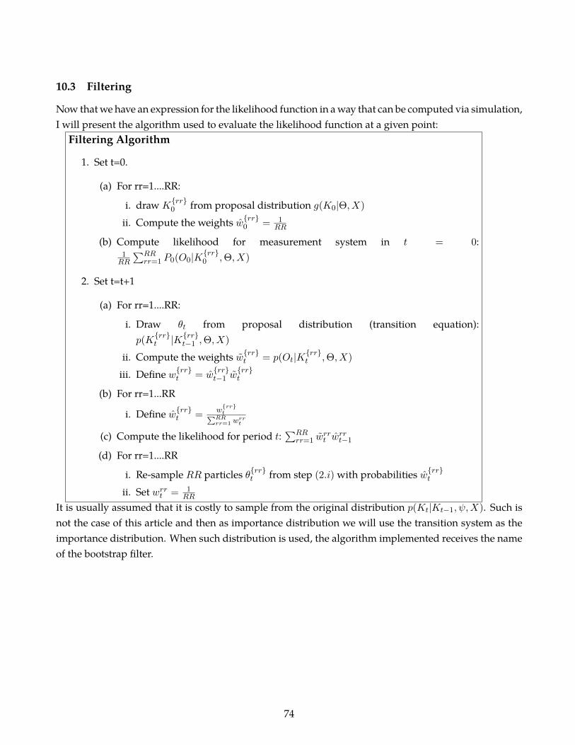
10.3 Filtering

Now that we have an expression for the likelihood function in a way that can be computed via simulation,I will present the algorithm used to evaluate the likelihood function at a given point:

Filtering Algorithm

1. Set t=0.

(a) For rr=1....RR:

i. draw Krr0 from proposal distribution g(K0|Θ, X)

ii. Compute the weights wrr0 = 1RR

(b) Compute likelihood for measurement system in t = 0:1RR

∑RRrr=1 P0(O0|Krr0 ,Θ, X)

2. Set t=t+1

(a) For rr=1....RR:

i. Draw θt from proposal distribution (transition equation):p(K

rrt |Krrt−1 ,Θ, X)

ii. Compute the weights wrrt = p(Ot|Krrt ,Θ, X)

iii. Define wrrt = wrrt−1 w

rrt

(b) For rr=1...RR

i. Define wrrt =wrrt∑RR

rr=1 wrrt

(c) Compute the likelihood for period t:∑RR

rr=1 wrrt w

rrt−1

(d) For rr=1....RR

i. Re-sample RR particles θrrt from step (2.i) with probabilities wrrt

ii. Set wrrt = 1RR

It is usually assumed that it is costly to sample from the original distribution p(Kt|Kt−1, ψ,X). Such isnot the case of this article and then as importance distribution we will use the transition system as theimportance distribution. When such distribution is used, the algorithm implemented receives the nameof the bootstrap filter.

74

Figure 18: Particle Filtering Algorithm

Figure 18 illustrates the particle filtering algorithm with eight particles. In the first step, particles aredrawn from the proposal distribution g(K0|Θ, X). In the second step, the likelihood of each particle isevaluated through the likelihood system P0 (O0|K0,Θ, X). In the third step, a new set of particles aredrawn with the corresponding weight given by the measurement system. Some particles might die andsome others are drawn multiple times.

75

10.4 Smoothing distribution

The smoothing distribution is useful if we are interested in making inference about the state of the un-observed factors. In this case, it is particularly interesting to make inference about the skills of children.The following procedure describes how to use the information provided in the model and in the data inorder to derive the smoothing distribution of the unobserved latent factors. This procedure is adaptedfrom Klaas et al. (2006):

I use as main input for this file the article ”Fast Particle Smoothing: If I had a Million Particles”. Itranslate the notation in the one used in the paper. Define O0:t = O0, O1..., Ot. The smoothed densityis:

p(Kt|O0:2) (85)

where we basically condition on all the measures we have. Note that we can write Equation 85 as:

p(Kt|O0:2) = p(Kt|O0:t)

∫ (p(Kt+1|O0:2)p(Kt+1|θt)∫p(Kt+1|θt)p(K1|O0:t)dKt

)dKt+1 (86)

And then we can approximate this distribution by p(θt|O0:2) with:

p(Kt|O0:2) =

RR∑rr=1

w(rr)t|T δK(rr)

t(Kt) (87)

where δK

(rr)t

(Kt) is the Dirac distribution and

w(mm)t|T = w

(mm)t

RR∑rr=1

w(rr)t+1|T

p(K

(rr)t+1 |K

(mm)t

)∑KK

kk=1w(kk)t p

(K

(rr)t+1 |K

(kk)t

) (88)

where wT |T = wT

Smoothing algorithm

1. For t=0,1,2 perform the particle filtering to obtain Krrt , w

rrt RRrr=1

2. Set wrr2|2 = wrr2 for rr = 1...RR

3. For t=1,0 define w(mm)t|2 = w

(mm)t

[∑RRrr=1w

(rr)t+1|2

(p(x(rr)t+1 |x

(mm)t

)∑KKkk=1 w

(kk)t p

(x(rr)t+1 |x

(kk)t

))]

76

Figure 19: Smoothing Distribution of Skills According to Household’s Income Percentile

The distribution of log(skills) is plotted for representative households. Households located in the 20th, 40th, 60th, 80th and 100th percentile of total householdincome. The smoothed distribution of all the households is presented in Figure 13

77

10.5 Cash Transfer Programs in Chile

The basic program through which poor families receive cash transfers from the central government isthe “Unique Family Subsidy”.20 Such program established a monthly transfer of $14,340 CLP in 2012, fora family in conditions of vulnerability21 with one child.22 The recipient of the transfer is always set to bethe mother of the children who generate the transfer. In addition to be within the 40% most vulnerable,in order for the mother should be economically inactive in order to receive the transfer. However, thealternate program “Family Assignment” cash transfers of the same value for those mothers who wereworking, with a fadeout scheme.23

In 2016, the basic amount of a transfer in the programs “Unique Family subsidy” and “Family Assign-ments” corresponded to $10,577. When compared to the $7,170 CLP of 2012, this represents an increaseof 29% in real terms. Additionally, in 2014 the government of Michelle Bachelet implemented the im-plemented the “Permanent Family Contribution Program”. In 2016, those families who were eligible toeither “Unique Family Subsidy” or “Family Assignments” were automatically eligible to be part of the“Permanent Family Contribution Program”. which consisted in a transfer of $43,042 anually for eachchildren and one for the family as a whole. Thus, a family one child would be eligible to receive $86,084CLP.

Overall, a family of one child that was receiving transfers from the “Unique Family Subsidy” programin 2012, would see an increase in the monetary transfers from the central government equivalent to 72.8%in real terms.

20Subsidio Unico familiar in Spanish.21The condition of vulnerability corresponds to a score below 11.734 in the “Ficha de ProtecciUn Social”. Approximately

40% of Chilean families lie below this threshold22The $14,340 CLP were generated by the mother and the child, each generating a transfer of $7,170 CLP.23The transfer scheme consisted of $7,179CLP for women with monthly wages below $187,515 CLP; $5,054 CLP for women

whose wages was in between $187,515 CLP and $307,863 CLP; and $1,600 CLP for women whose wages was between $307,863CLP and $480,163.

78