Evaluating Demand for Courses at UC Berkeley

Matthew Symonds Economics Honors Thesis, UC Berkeley, May 2015

Advisor: Professor Chris Shannon

Abstract: This paper analyzes the welfare costs of waitlists and oversubscription of courses at UC Berkeley. First, using theory, it shows how understanding the probability of successful enrollment off a waitlist could guide superior enrollment decisions. Second, using data, it analyzes predictors of enrollment differences in similar courses and concludes that professor ratings and course times play a role in explaining why waitlists accumulate in certain courses and not others.

Acknowledgements: Thank you to Professor Shannon (Math/Economics), Professor Bart Hobjin (Economics), the berkeleytime.com team Yuxin Zhu (Computer Science 2015), Noah Gilmore (Electrical Engineering and Computer Science 2015), and Ashwin Iyengar (Astrophysics and Computer Science 2016) for all the help you provided.

1/14

0: Introduction We can think of the course enrollment process at UC Berkeley as a market, where the demand for a course is the number of students who wish to enroll, and the supply is the number of seats in the course available. Undergraduate students use the Web Page Tele­Bears to sign up for the courses they wish to take, but there are often not enough seats to accommodate everyone in a given semester. When demand exceeds supply, a student may join the waitlist to enroll, with no guarantee she will get to enroll. In the College of Letters and Sciences, 373 courses of 2,879 in Spring 2015, and 403 of 2,864 courses in Spring 2014, were impacted, meaning they turned away students, sometimes in the dozens. Satisfaction with the course enrollment process is low. In April 2010, the university hired Bain & Company to identify inefficiencies and mismanagement in university administration. In their report, the consultancy highlighted a survey response that “the TeleBEARS system should be made less confusing. It doesn’t help students design schedules easily. Currently it is a nightmare to use.” The Bain & Company report prompted a university­wide initiative, called “Operational Excellence,” meant to improve university administrative processes and save money. This initiative will tackle the course enrollment process at some stage. An analysis of the welfare effects of the course enrollment process could be useful to those seeking to improve enrollment outcomes for students. Waitlists reflect two visible kinds of inefficiency in the course market. First, students who waitlist courses and are turned away experience a welfare cost as they forgo course opportunities to join a waitlist, only to fail to enroll. Second, the very mechanism of a waitlist depends on students dropping a course. I argue that most students change their course schedule based on information not initially available. Lack of good information imposes a welfare cost on students, either because they join the courses in which they wish to enroll late, or, courses that, with better information, they could have chosen initially are no longer available. We shall analyze both of these inefficiencies in turn.

1: Welfare Cost of Waitlist Uncertainty In this section we will develop a model to illustrate the welfare cost of waitlist uncertainty on students. Second, we develop a procedure for estimating the probability of getting off the waitlist for a given course.

2/14

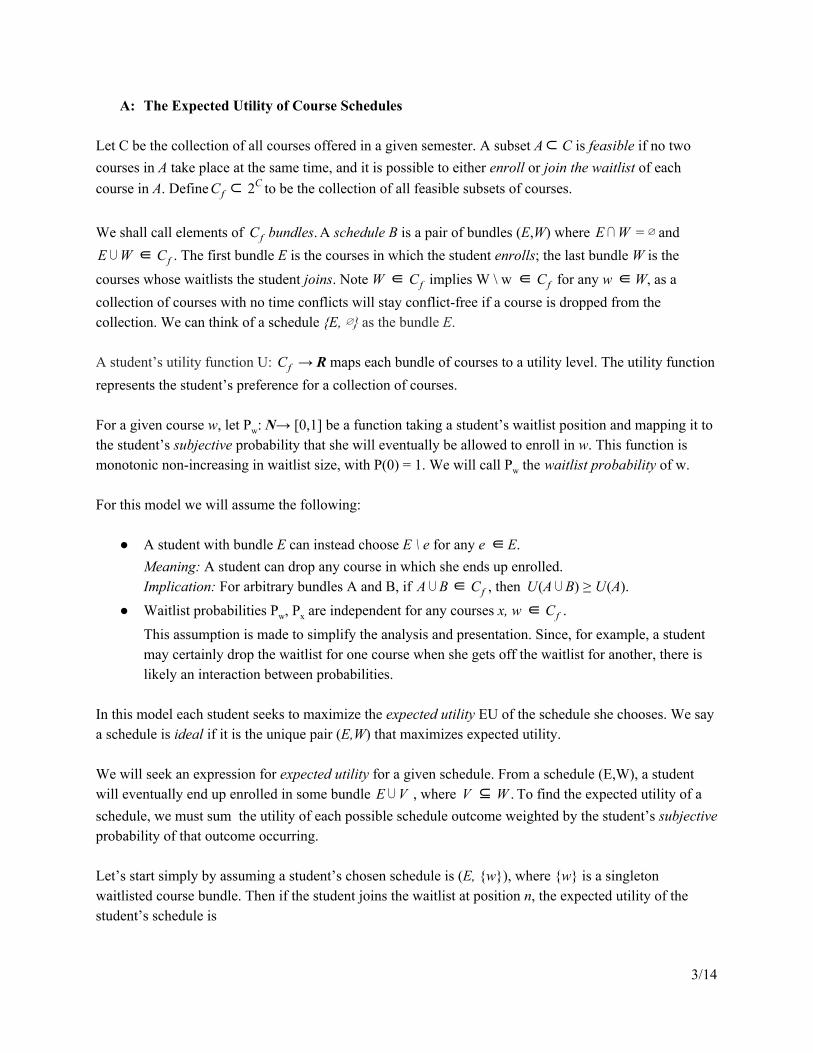
A: The Expected Utility of Course Schedules Let C be the collection of all courses offered in a given semester. A subset A C is feasible if no two⊂ courses in A take place at the same time, and it is possible to either enroll or join the waitlist of each course in A. Define to be the collection of all feasible subsets of courses.C f ⊂ 2C We shall call elements of bundles.

A schedule B is a pair of bundles (E,W) where andC f E⋂W = ∅ . The first bundle E is the courses in which the student enrolls; the last bundle W is theE⋃W ∈ C f

courses whose waitlists the student joins. Note W implies W \ w for any w W, as a∈ C f ∈ C f ∈ collection of courses with no time conflicts will stay conflict­free if a course is dropped from the collection. We can think of a schedule E, ∅ as the bundle E. A student’s utility function U: → R maps each bundle of courses to a utility level. The utility functionC f represents the student’s preference for a collection of courses. For a given course w, let Pw: N→ [0,1] be a function taking a student’s waitlist position and mapping it to the student’s subjective probability that she will eventually be allowed to enroll in w. This function is monotonic non­increasing in waitlist size, with P(0) = 1. We will call Pw the waitlist probability of w. For this model we will assume the following:

A student with bundle E can instead choose E \ e for any e E.∈ Meaning: A student can drop any course in which she ends up enrolled. Implication: For arbitrary bundles A and B, if , then A⋃B∈ C f (A ) (A).U ⋃B ≥ U

Waitlist probabilities Pw, Px are independent for any courses x, w .∈ C f This assumption is made to simplify the analysis and presentation. Since, for example, a student may certainly drop the waitlist for one course when she gets off the waitlist for another, there is likely an interaction between probabilities.

In this model each student seeks to maximize the expected utility EU of the schedule she chooses. We say a schedule is ideal if it is the unique pair (E,W) that maximizes expected utility. We will seek an expression for expected utility for a given schedule. From a schedule (E,W), a student will eventually end up enrolled in some bundle , where To find the expected utility of aE⋃V .V ⊆ W schedule, we must sum the utility of each possible schedule outcome weighted by the student’s subjective probability of that outcome occurring. Let’s start simply by assuming a student’s chosen schedule is (E, w), where w is a singleton waitlisted course bundle. Then if the student joins the waitlist at position n, the expected utility of the student’s schedule is

3/14

EU[(E, w)] = [1].(n) U (B w) (1 (n))U (B) Pw ⋃ + − Pw

So the expected utility of the schedule is the sum of the utility of the bundle with w and the utility of the bundle without w, weighted by the probability of the student ending up enrolled in either. Now let’s expand to two waitlisted courses w1 and w2 with length m and n. Since waitlist probabilities for different courses are independent, the expected utility is as follows: EU[(E,w1,w2)] = (n) (1 (m)) U (B w ) + Pw1 − Pw2 ⋃ 1

(m) (1 (n)) U (B w ) + Pw2 − Pw1 ⋃ 2

[2]. (1 (n))(1 (m)) U (B) + − Pw1 − Pw2 There are four possible outcomes in this scenario: the student enrolls in w1 and w2, she enrolls in w1, she enrolls in w2, or she enrolls in neither. The utilities of each of these outcomes is weighted by their probabilities. We could expand this formula to three waitlisted courses, but it turns out the general form for an arbitrary number waitlists is pretty and more informative. For schedule (E,W), the expected utility formula is

[3],EU[(E, )] (E ) P(E ) W = ∑

V∈ 2WP ⋃V ⋃V

where V becomes every possible subset of W. In other words, the sum covers every possible way waitlisting the courses in W could turn out for the student. To end up with E U V, the student has to successfully enroll in each course in V and fail to enroll in each course in W \ V. So the probability of attaining E U V is equal to the probability of successfully enrolling in each course in V, times the probability of failing to enroll in each course in W \ V. Since we assumed waitlist probabilities are independent, we can decompose each outcome’s probability into a product of waitlist probabilities. Using individual enrollment probabilities in the expected utility expression yields the following formula:

∑

V∈2W(n ) U (E )[ ∏

b ∈ i : w ∈ V i

P b b ∏

c ∈ j: w ∈ W∖V j

1 (n )[ − P c c ] ⋃V ] 4]. [

Note there are 2|W| summands in this formula. Next, there are |V| probability terms in the left product, and

|W \ V| terms in the right product. In total, there are 2|W| (|V| + |W \ V|), or |W| (2|W|), probability terms used to determine expected utility when waitlisted in |W| courses.

4/14

Recall, though, that the probability terms here driving the student’s actions are the student’s subjective probability of enrollment. It could be the student’s estimates are inaccurate. In short, the accuracy of the probability value itself matters quite a bit when evaluating the schedule’s expected utility:

# Probability Terms in Expected Utility of (E,W)

Waitlisted Courses |W| 1 2 3 4 5 [5].

# Probability Terms Pw 2 8 24 64 160 To explore this idea, let’s denote accurate probabilities with an asterisk, and suppose Pw* = 0 for a waitlisted course w W and P* = P for all other courses. If the student selects schedule (E,W)∈ considering his subjective probabilities but an alternative schedule (F,X) maximizes expected utility using accurate probabilities, then the expected welfare cost for the student selecting schedule (E,W) is EU[(F,X)] ­ EU[(E, )] .∖w W ≥ 0 Is this welfare cost strictly positive? One reason to think so is that the the schedule (F,X) can include any course whose time overlaps with w’s time, while (E, ) cannot since (E,W) had to be feasible. Find∖w W one course a with open seats that the student would wish to take had she not taken w. We can construct (F,X) = (E , W \ w) and in this case we conclude EU[(F,X)]­ EU[(E,W \ w)] > 0.⋃a A more specific example follows. Consider a course, like first semester calculus (Math 1A), that has two lecture sections, one with a waitlist and one with open seats. Suppose a student wants Math 1A in her schedule and prefers the waitlisted section. If she overestimates her chances of enrollment, joins the waitlisted section, and subsequently is required to drop the course, there is clear welfare cost. A near­perfect substitute schedule existed that the student certainly would have preferred if she knew her true chances of enrollment. The model also highlights a complementary, but invisible, welfare cost of waitlist uncertainty. Suppose a student wishes to enroll in w, and his ideal schedule is (E,w). If Pw = 0, but Pw* = 1, the student will not enroll in w even though using accurate probabilities he has a 100% chance of obtaining his ideal schedule. Since he enrolls in (F,X) where his welfare cost is EU[(E,w)] ­ EU[(F,X)] > 0.∈ , w / F Why is this cost invisible? Suppose students s1 and s2 choose schedule (F, . On the first day, they meet)Ø and notice they have the exact same schedule. Student s1 says, “The only reason I’m taking f is because w had a long waitlist, and I didn’t think I would get in.” Student s2 says, “Really? You wanted to take w instead of f? I couldn’t be more excited for f. My schedule is ideal.” Consider s1’s situation in this story. He believes Pw(n) ≈ 0. Suppose the accurate probability P*w(n) is equal to 1. Then s1 has suffered a positive welfare cost EU[(F \ f,w)] ­ EU[(F, )]. Meanwhile, theØ welfare loss of student s2 is 0, because he achieved his ideal schedule.

5/14

On paper s1 and s2 are indistinguishable, but their welfare loss because of waitlist uncertainty is not the same. Because s1’s action’s did not indicate any interest in taking w, we can’t find out he was interested with enrollment statistics alone. Both welfare effects, from inappropriate acceptance of a waitlist and inappropriate avoidance of a waitlist, could be mitigated with better information about the probability of getting off the waitlist for a given course.

B: Empirical Probabilities and the 10% Rule of Thumb The “10%” Rule of Thumb is a guideline students often use to assess their chances of enrollment. This rule of thumb says if the waitlist size is less than 10% of the course enrollment, then one’s chances of getting off the waitlist are good. It’s a guideline used as advice by the university’s Golden Bear Blog and one I have heard repeated on campus. Since it is widespread, this rule could be the subjective probability function used by many students. A natural next step, then, would be to estimate if this rule of thumb is accurate using past data. If we can confirm or disconfirm the rule of thumb, this new information could provide guidance to students seeking to improve the welfare properties of their course enrollment strategy. First, we need to develop a procedure for constructing empirical probability functions, using past semesters’ data. Let C be the previous semester’s courses. Conduct the following procedure for each course c For.∈ C each waitlist position k, count the the number of students up to and including the first student to join the kth position on the waitlist who:

successfully enrolled in the course (1), fails to leave the waitlist and is turned away (2), or voluntarily drops the waitlist for any reason (3).

If the counts sum (1) + (2) = 0, then set P*(k) = . Otherwise, set 1

P*(k) =(1)

(1) + (2) 6]. [ This empirical probability function P* is the historic proportion of students who successfully enrolled from the initial waitlist, among those who wished to enroll, with an adjustment for lack of data. The procedure described above is the ideal way to calculate accurate an empirical probability estimate for the student’s use. To create richer results, the procedure could be tweaked to count the sum enrollment outcomes from a collection of courses deemed similar, for instance, all 9am lectures of Econonomics 1 from past semesters’ data.

6/14

The construction gives us monotonicity for free. If the first student who joined the waitlist at position 6 fails to enroll, then the first position­holder at position 7 and later will fail to enroll as well, pushing the probability down. We count the outcome of initial waitlist position­holders only because it prevents late joiners from skewing the probability of a low waitlist position. Implicitly, their waitlist position is the number of all people on the waitlist before him who left the waitlist. (To accommodate late joiners, we could construct a function like P*(k,t) that takes time period t into account, but that won’t be our focus.) It’s worth emphasizing that P* is not a probability distribution; it is an empirically constructed probability function mapping waitlist positions to probabilities of enrollment. Waitlist position is given, and not the

outcome, so there’s no requirement that (k) 1.∑n

k = 0P * =

The 10% Rule of Thumb can be stated as follows: If you join the waitlist of course c at position k where k is less than 10% of the max enrollment of c, you’re more likely than not to get off the waitlist and enroll in the course. Let C10% be the set of courses whose waitlists exceed 10% of maximum enrollment. To test the rule of thumb, take as the sample the collection of all P*(k) from every c C10%,. The null hypothesis H0 is∈ P*(k) while the alternative hypothesis H1 is P*(k) > 0.5, the rule of thumb. The one­sided t­test is.5,≤ 0 appropriate here. Over P*(k) calculate a mean, a standard error, and a t­value, finally calculating the p­value. If p < 0.05 then reject the null hypothesis in favor of the rule of thumb H1. The sample is size |C10%|. In theory this could be too small to achieve statistical significance. C10% could even be empty. That would make the 10% Rule of Thumb vacuous, kind of like a rule of thumb for thesis length at Hogwarts. In practice, this is not a concern, as |C10%| >> 0. Unfortunately, a more fundamental barrier exists. This statistical test, and any probability estimate, won’t be possible unless the university begins tracking data on the reasons students drop courses, particularly waitlists. The data the university collects, and even better data collected by outside sources, does not indicate why the waitlist went down, only when and by how much. The lack of data on reasons people leave waitlists poses a barrier to estimating the probability function of each waitlist. Without the data, this paper cannot make any estimates to test the 10% Rule of Thumb or any other hypothesis.

C: Discussion and Recommendation In this section we developed an argument that good estimates of the probability of getting off waitlists can assist students who wish to improve their course enrollment outcomes and mitigate the welfare costs of oversubscription of courses. A procedure was developed for estimating these probabilities given data on student enrollment outcomes after joining a given waitlist. My recommendation is that the University begin collecting this data.

7/14

Currently there are plans to update the course enrollment process. The University is currently undergoing an update of shared technology services as part of a wider initiative to improve the efficiency and quality of campus administration and services. Dubbed “Operational Excellence,” this initiative has already replaced the course portal Web Page bSpace with bCourses, and improvments to Tele­Bears, including improved data collection, are underway. This data should include for each course individual level data on the following:

1) What were the positions of students on the waitlist who enrolled? 2) What were the positions of students on the waitlist who voluntarily dropped? 3) What were the positions of students on the waitlist who were turned away?

With this data, the university will be empowered to deliver good information to students on enrollment outcomes, helping students make good decisions about which courses to waitlist.

2: Predicting Excess Demand for Courses So far we have identified two costs to waitlists:

1) The cost of waitlists on those who join them and are turned away, and 2) The cost of waitlists on those who wish to enroll in a course but are discouraged from doing so,

even though they had a good shot of enrollment if they tried. Recall 2) is invisible to the university unless they begin collecting survey data. Waitlists are indicative of a third welfare cost that students experience, which we will explore. This cost, summed with 1), suggests that the length of a waitlist, and the length of the duration of a waitlist, are a floor for the number of students in the course who experience a welfare loss due to enrollment.

A: Aggregate Welfare Costs of Over­Enrollment Suppose a student is at position k on a waitlist. Suppose a students drop who are enrolled, b students drop from the waitlist ahead of position k. In order for the student at position k to enroll, it must be the case that a + b . If k is the last position of a student who enrolls in the course, and the waitlist is length n, then n≥ k ­ k students were turned away from the waitlist. Thus the number of students who were turned away or decided to drop a course is

n ­ k + (a + b) [7]. ≥ n

The existence of a waitlist length n guarantees at least n students will not complete the course they initially enrolled or waitlisted. Thus the length of a waitlist indicates how many students will be

8/14

disappointed by their schedule selection at some point, and thus indicates the minimum number of students in a course who have selected sub­optimal schedules. Each of the n students experiences an opportunity cost to the time they invested in the course. During the time they spent attending lectures, studying, and doing homework, they could have been studying for other courses, or honing their backgammon skills. We can broadly think of opportunity cost of time invested as proportional to the number of days the student was enrolled before leaving the course. In other words, from a welfare perspective it is plainly better for a course to accumulate a waitlist of 100 students on day 5, and have all of them turned away or enrolled on day 10, than it is for the 100 person waitlist to persist until day 55, after which the waitlist is flushed. Some rejected students may find their partial experience in the course they waitlisted valuable. However, the time a student invested in the course she waitlisted could have been used productively towards attending another course and obtaining a grade, so it’s not plausible the student’s best welfare scenario is being waitlisted and turned away. Here we make the reasonable assumption that students who enroll and pay tuition seek certification for their education in addition to the education itself.

B. Predicting Excess Demand

Understanding that long waitlists, that endure for long periods of time, are bad for welfare, our next step is to analyze the factors that drive waitlist length and duration. For each course, we could attempt to predict the parameter

[8],(c) D = M−1∑

t W t

where D stands for Welfare Distress, c is a given course, M is the sum of course’s max enrollment and its max waitlist size, while Wt is the waitlist length on day t. Suppose c1 and c2 are close substitutes, e.g. they’re two sections of Economics 100A. Then it would be particularly interesting to measure

[9],(c ) D(c ) (c ) (c ) (c ) (c )D 1 − 2 = M−11 ∑

t W t 1 −M−1

2 ∑

t W t 2

since this discrepancy in distress between two similar courses could indicate a welfare improvement is possible by making the course with higher oversubscription more similar to the course with lower oversubscription. A student leaving a course they initially enrolled in may indicate an information problem, where the student later obtains information that makes her change her mind about enrollment. Therefore when

9/14

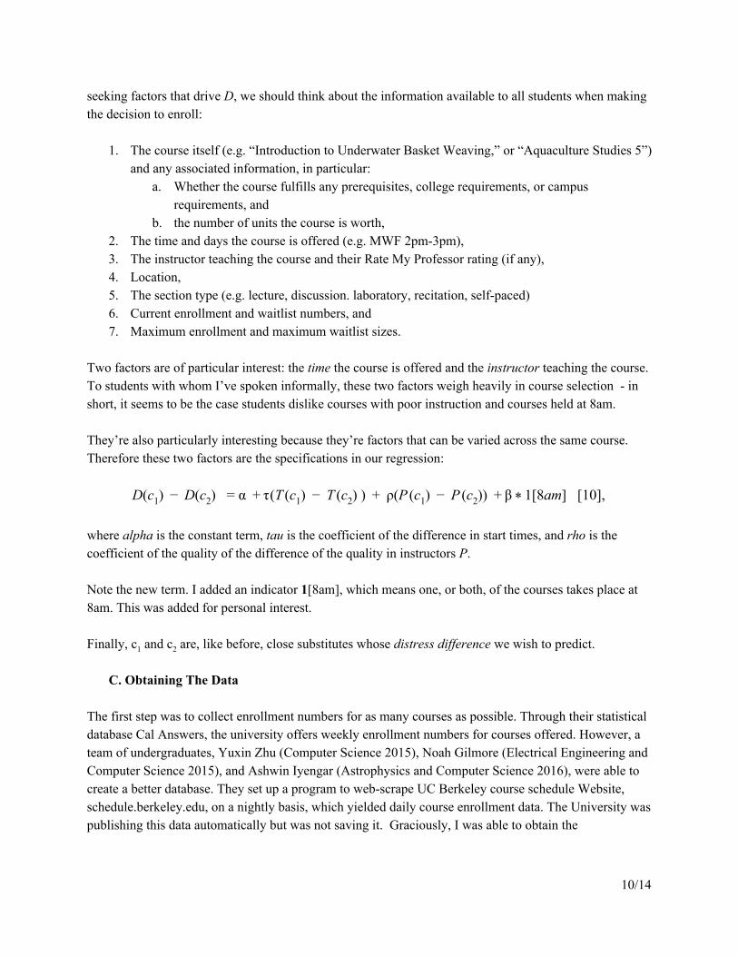
seeking factors that drive D, we should think about the information available to all students when making the decision to enroll:

1. The course itself (e.g. “Introduction to Underwater Basket Weaving,” or “Aquaculture Studies 5”) and any associated information, in particular:

a. Whether the course fulfills any prerequisites, college requirements, or campus requirements, and

b. the number of units the course is worth, 2. The time and days the course is offered (e.g. MWF 2pm­3pm), 3. The instructor teaching the course and their Rate My Professor rating (if any), 4. Location, 5. The section type (e.g. lecture, discussion. laboratory, recitation, self­paced) 6. Current enrollment and waitlist numbers, and 7. Maximum enrollment and maximum waitlist sizes.

Two factors are of particular interest: the time the course is offered and the instructor teaching the course. To students with whom I’ve spoken informally, these two factors weigh heavily in course selection ­ in short, it seems to be the case students dislike courses with poor instruction and courses held at 8am. They’re also particularly interesting because they’re factors that can be varied across the same course. Therefore these two factors are the specifications in our regression:

(c ) D(c ) (T (c ) T (c ) ) ρ(P (c ) P (c )) [8am] [10], D 1 − 2 = α + τ 1 − 2 + 1 − 2 + β * 1 where alpha is the constant term, tau is the coefficient of the difference in start times, and rho is the coefficient of the quality of the difference of the quality in instructors P. Note the new term. I added an indicator 1[8am], which means one, or both, of the courses takes place at 8am. This was added for personal interest. Finally, c1 and c2 are, like before, close substitutes whose distress difference we wish to predict.

C. Obtaining The Data The first step was to collect enrollment numbers for as many courses as possible. Through their statistical database Cal Answers, the university offers weekly enrollment numbers for courses offered. However, a team of undergraduates, Yuxin Zhu (Computer Science 2015), Noah Gilmore (Electrical Engineering and Computer Science 2015), and Ashwin Iyengar (Astrophysics and Computer Science 2016), were able to create a better database. They set up a program to web­scrape UC Berkeley course schedule Website, schedule.berkeley.edu, on a nightly basis, which yielded daily course enrollment data. The University was publishing this data automatically but was not saving it. Graciously, I was able to obtain the

10/14

undergraduate database for this analysis. The data is also visualized at the course enrollment section of their Website, berkeleytime.com. The next step was to determine a way to quantify instructor quality P(c). Since students cannot know an instructor’s style of instruction until they enroll, it is more important to the analysis to obtain some measure of perceived quality. Rate My Professors is a popular instructor rating Website, holding an Alexa Website popularity ranking of 787 in the United States. The Berkeley page is popular as well, with over 3,000 professors rated. Students log in to rate their instructors on a scale from 1­to­5 on helpfulness, clarity, and easiness, which are aggregated into an overall ranking between 1 and 5. (Instructors are also rated “hot or not,” but for the purposes of this regression specification that that ranking was excluded.) To obtain the Rate My Professor data, the alphabetical list of professors available at http://www.ratemyprofessors.com/campusRatings.jsp?sid=1072 was manually scrolled all the way to the bottom to include every professor’s name and their aggregate ranking. Then the Website was saved and each professor’s name and rating was scraped into a table.

D. Regression Out of 24,747 lectures, discussions, laboratories, recitation periods, and self­paced courses offered in Spring 2013 through Spring 2015, 2,501 pairs of sections were selected that shared the same course (e.g. Math 1A), the same kind of section (e.g. lecture), were offered on the same days in the same semester of the same year, and for which enrollment data was available for both during the same period. Time differences and Rate My Professor score differences were calculated. Then the sum of the waitlist was divided by the sum of maximum enrollment and maximum waitlist size for each course. The results of the regression are as follows: Table [11]: Regression of Time Difference and RMP Score Difference on Distress Difference in Pairs of Substitutable Courses (n = 2,501)

Variable D1 ­ D2 SE p

Constant ­0.02844 0.08972 0.7513 T(c1) ­ T(c2) 0.04271 0.02603 0.1009

P(c1) ­ P(c2) 1.01835 0.61099 0.0957` 1(8am) 0.26166 0.23318 0.2619 R2 = 0.002743 F = 2.289 (p = 0.07651)

` indicates p < 0.1 The most significant result in the regression is the professor’s score difference effect. At p = 9%, the regression suggests that a one point difference in scores can lead to a one point difference in distress. Examining the first row, the regression reveals is not a strong relationship between the time difference and

11/14

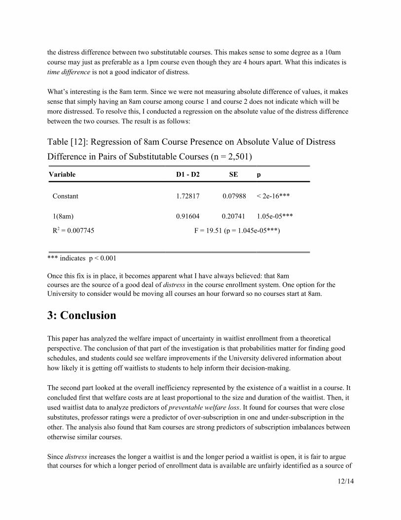
the distress difference between two substitutable courses. This makes sense to some degree as a 10am course may just as preferable as a 1pm course even though they are 4 hours apart. What this indicates is time difference is not a good indicator of distress. What’s interesting is the 8am term. Since we were not measuring absolute difference of values, it makes sense that simply having an 8am course among course 1 and course 2 does not indicate which will be more distressed. To resolve this, I conducted a regression on the absolute value of the distress difference between the two courses. The result is as follows: Table [12]: Regression of 8am Course Presence on Absolute Value of Distress Difference in Pairs of Substitutable Courses (n = 2,501)

Variable D1 ­ D2 SE p

Constant 1.72817 0.07988 < 2e­16***

1(8am) 0.91604 0.20741 1.05e­05***

R2 = 0.007745 F = 19.51 (p = 1.045e­05***)

*** indicates p < 0.001 Once this fix is in place, it becomes apparent what I have always believed: that 8am courses are the source of a good deal of distress in the course enrollment system. One option for the University to consider would be moving all courses an hour forward so no courses start at 8am.

3: Conclusion This paper has analyzed the welfare impact of uncertainty in waitlist enrollment from a theoretical perspective. The conclusion of that part of the investigation is that probabilities matter for finding good schedules, and students could see welfare improvements if the University delivered information about how likely it is getting off waitlists to students to help inform their decision­making. The second part looked at the overall inefficiency represented by the existence of a waitlist in a course. It concluded first that welfare costs are at least proportional to the size and duration of the waitlist. Then, it used waitlist data to analyze predictors of preventable welfare loss. It found for courses that were close substitutes, professor ratings were a predictor of over­subscription in one and under­subscription in the other. The analysis also found that 8am courses are strong predictors of subscription imbalances between otherwise similar courses. Since distress increases the longer a waitlist is and the longer period a waitlist is open, it is fair to argue that courses for which a longer period of enrollment data is available are unfairly identified as a source of

12/14

welfare loss. My response is that the approach taken is fairest given the data available. To extrapolate from a short period of enrollment data from a course would be inappropriate because it may have been the case that enrollment closed. The only welfare loss for which there is evidence is the loss reflected in the data. Some may wonder whether certain departments have higher inefficiency to enrollment than others. This would be an area of further analysis. Departments could certainly take a similar approach as that taken in this paper to identify courses that are over­or­under­subscribed and factors that are driving that discrepancy. In particular, the Physics department does not permit the existence of waitlists, and many language departments resolve oversubscription by placing everyone into the waitlist initially, then filtering students by prerequisite completion. Further investigation is needed to determine whether these strategies help or hinder students. Efforts to collect the data necessary to improve the course enrollment process would certainly be consistent with the objectives outlined in the university’s Operational Excellence initiative. As is evident from Berkeley’s course enrollment situation and the analysis developed in this paper, improving welfare outcomes for students by improving course enrollment is a fruitful area of investigation.

13/14

4: References Achieving Operational Excellence at University of California, Berkeley. Rep. San Francisco:

Bain, CA. Final Diagnostic Report. Web. 1 Apr. 2015.

http://oe.berkeley.edu/sites/default/files/diagnostic%20report%20bain%20uc%20berkel

ey.pdf.

Nevels, Lyle, Shel Waggener, and Paul Wright. Design Phase Business Case. Rep. Berkeley: UC

Berkeley, CA. OE Information Technology Design Initiative. Operational Excellence.

Web. 29 May 2015.

http://oe.berkeley.edu/sites/default/files/I_BusCase_041211.pdf

Schiffer, Emma. "Navigating The Waitlist." Web log post. Golden Bear Blog. UC Berkeley, 14

July 2014. Web. 25 May 2015.

"Weekly Enrollment Management ­ Class Tracking." Cal Answers. UC Berkeley, 1 Apr. 2015.

Web. 1 Apr. 2015.

http://calanswers.berkeley.edu

Zhu, Yuxin, Noah Gilmore, and Ashwin Iyengar. "Course Discovery. Simplified." Berkeleytime.

N.p., 19 Mar. 2015. Web. 19 Mar. 2015.

http://www.berkeleytime.com. Authors provided the course database on the website

directly.

14/14