Evaluating Complexity, Code Churn, and Developer Activity Metrics as Indicators of Software

> REPLACE THIS LINE WITH YOUR PAPER IDENTIFICATION NUMBER (DOUBLE-CLICK HERE TO EDIT) <

1

Abstract—Security inspection and testing requires experts in security who think like an attacker. Security experts need

to know code locations on which to focus their testing and inspection efforts. Since vulnerabilities are rare occurrences, locating vulnerable code locations can be a challenging task. We investigated whether software metrics obtained from source code and development history are discriminative and predictive of vulnerable code locations. If so, security experts can use this prediction to prioritize security inspection and testing efforts. The metrics we investigated fall into three categories: complexity, code churn, and developer activity metrics. We performed two empirical case studies on large, widely-used open source projects: the Mozilla Firefox web browser and the Red Hat Enterprise Linux kernel. The results indicate that 24 of the 28 metrics collected are discriminative of vulnerabilities for both projects. The models using all the three types of metrics together predicted over 80% of the known vulnerable files with less than 25% false positives for both projects. Compared to a random selection of files for inspection and testing, these models would have reduced the number of files and the number of lines of code to inspect or test by over 71% and 28%, respectively, for both projects.

Index Terms-- Software security, Software metrics, Vulnerability prediction, Fault prediction.

I. INTRODUCTION

single exploited software vulnerability1 can cause severe damage to an organization.

Annual world-wide losses caused from cyber attacks have been reported to be as high as $226

billion [2]. Loss in stock market value in the days after an attack is estimated at $50 million to

$200 million per organization [2]. The importance of detecting and mitigating software

vulnerabilities before software release is paramount.

Experience indicates that the detection and mitigation of vulnerabilities is best done by

engineers specifically trained in software security and who “think like an attacker” in their daily

Manuscript received March 18, 2009. This work was supported in part by National Science Foundation Grant No. 0716176 and the U.S.

Army Research Office (ARO) under grant W911NF-08-1-0105 managed by NCSU Secure Open Systems Initiative (SOSI). Y. Shin is with North Carolina State University, Raleigh, NC 27695 USA (telephone: 919-946-0781, e-mail: yonghee.shin@ ncsu.edu). A. Meneely is with North Carolina State University, Raleigh, NC 27695 USA (e-mail: [email protected]). L. Williams is with North Carolina State University, Raleigh, NC 27695 USA (e-mail: [email protected]). J. Osborne is with North Carolina State University, Raleigh, NC 27695 USA (e-mail: [email protected]). 1 An instance of a [fault] in the specification, development, or configuration of software such that its execution can violate an

[implicit or explicit] security policy [1]

Evaluating Complexity, Code Churn, and Developer Activity Metrics as Indicators of

Software Vulnerabilities Yonghee SHIN, Student Member, IEEE, Andrew MENEELY, Student Member, IEEE,

Laurie WILLIAMS, Member, IEEE, and Jason OSBORNE

A


2

work [3]. Therefore, security testers need to have specialized knowledge in and a mindset for

what attackers will try. If we could predict which parts of the code are likely to be vulnerable,

security experts can focus on these areas of highest risk. One way of predicting vulnerable

modules is to build a statistical model using software metrics that measure the attributes of the

software products and development process related to software vulnerabilities. Historically,

prediction models trained using software metrics to find faults have been known to be effective

[4-10].

However, prediction models must be trained on what they are intended to look for. Rather

than arming the security expert with all the modules likely to contain faults, a security prediction

model can point toward the set of modules likely to contain what a security expert is looking for:

security vulnerabilities. Establishing predictive power in a security prediction model is

challenging because security vulnerabilities and non-security-related faults have similar

symptoms. Differentiating a vulnerability from a fault can be nebulous even to a human, much

less a statistical model. Additionally, the number of reported security vulnerabilities with which

to train a model are few compared to non-security-related faults. Colloquially, security

prediction models are “searching for a needle in a haystack.”

In this paper, we investigate the applicability of three types of software metrics to build

vulnerability prediction models: complexity, code churn, and developer activity metrics.

Complexity can make code difficult to understand and to test for security. Frequent or large

amount of code change can introduce vulnerabilities. Poor developer collaboration can diminish

project-wide secure coding practices.

The goal of this study is to guide security inspection and testing by analyzing if Complexity,

Code churn, and Developer activity (CCD) metrics can be used to (a) discriminate between


3

vulnerable and neutral files, and (b) predict vulnerabilities. For this purpose, we performed

empirical case studies on two widely-used, large scale open source projects: the Mozilla Firefox2

web browser and the Linux kernel as distributed in Red Hat Enterprise Linux3. We analyzed

Mozilla Firefox and Red Hat Enterprise Linux (each of them containing over two million lines of

source code), and evaluated the adequacy of using CCD metrics as indicators of security

vulnerabilities. We also measured the reduction in code inspection effort using CCD metrics

against random file selection.

The rest of the paper is organized as follows: Section II defines background terms. Section III

provides our hypotheses and the methodology for our case studies. In Sections IV and V, we

provide the results from both case studies. Section VI provides the summary of results from the

case studies and discusses issues in the use of models in practice. Section VII discusses the

threats to validity of our study. Section VIII provides related work. Section IX contains

conclusions and future work.

II. BACKGROUND

This section describes the background on discriminative power, predictability, network

analysis, and the binary classification evaluation criteria that we will use in this paper.

A. Discriminative Power and Predictability

This study investigates the discriminative power and predictability of CCD metrics in the

realm of software security. Discriminative power [11] is defined as the ability to “discriminate

between high-quality software components and low-quality software components”. In our study,

discriminative power is the ability to discriminate the vulnerable files from neutral files. We

2 http://www.mozilla.com/firefox/ 3 http://www.redhat.com/rhel/


4

classify a file as vulnerable if it has been fixed post-release for a vulnerability and as neutral file

if no vulnerabilities have been found at the time of our analysis.

Predictability [11] is the ability of a metric to identify files that are likely to have

vulnerabilities with metric values available prior to software release. Note that discriminative

power is measured for a single metric with the vulnerability information available at the present

time for the purpose of controlling the metric values by redesign or re-implementation or to

investigate the feasibility of building prediction models using the given metrics. On the other

hand, predictability can be measured using single or multiple metrics together and the data

obtained from past and present is applied to predict the code locations that are likely to have

vulnerabilities in the future.

B. Network Analysis

In this paper, we use several terms from network analysis [12] and provide their meaning with

respect to developer and contribution networks that will be discussed in Section III.A. Network

analysis is the study of characterizing and quantifying network structures, represented by graphs

[12]. A sequence of non-repeating, adjacent nodes is a path, and a shortest path between two

nodes is called a geodesic path (note that geodesic paths are not necessarily unique).

Centrality metrics are used to quantify the location of one node relative to other nodes in the

network. The centrality metrics we use for developer activity are degree, closeness, and

betweenness. The degree metric is defined as the number of neighbors directly connected to a

node. The closeness centrality of node is defined as the average distance from to any other

node in the network that can be reached from . The betweenness centrality [12] of node is

defined as the number of geodesic paths that include .

Cluster metrics are used to measure the strength of interconnection between groups of nodes.


5

A cluster of nodes is a set of nodes such that there are more edges within a set of nodes (intra-set

edges) than edges between a set and other sets of nodes (inter-set edges). The cluster metric we

use for developer activity is edge betweenness [13]. The edge betweenness of edge e is defined

as the number of geodesic paths that pass through e. Since clusters have many intra-cluster

edges, edges within clusters have a low betweenness; conversely, edges between two clusters

have a high betweenness [13].

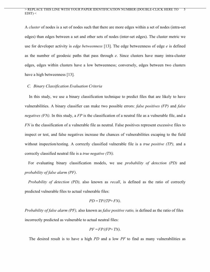
C. Binary Classification Evaluation Criteria

In this study, we use a binary classification technique to predict files that are likely to have

vulnerabilities. A binary classifier can make two possible errors: false positives (FP) and false

negatives (FN). In this study, a FP is the classification of a neutral file as a vulnerable file, and a

FN is the classification of a vulnerable file as neutral. False positives represent excessive files to

inspect or test, and false negatives increase the chances of vulnerabilities escaping to the field

without inspection/testing. A correctly classified vulnerable file is a true positive (TP), and a

correctly classified neutral file is a true negative (TN).

For evaluating binary classification models, we use probability of detection (PD) and

probability of false alarm (PF).

Probability of detection (PD), also known as recall, is defined as the ratio of correctly

predicted vulnerable files to actual vulnerable files:

PD =TP/(TP+FN).

Probability of false alarm (PF), also known as false positive ratio, is defined as the ratio of files

incorrectly predicted as vulnerable to actual neutral files:

PF =FP/(FP+TN).

The desired result is to have a high PD and a low PF to find as many vulnerabilities as


6

possible without wasting inspection or testing effort. Having a high PD is especially important

in software security considering the potentially high impact of a single exploited vulnerability.

Additionally, we provide precision (P), defined as the ratio of correctly predicted vulnerable files

to all detected files:

P =TP/(TP+FP).

We report P with PD as they tend to trade-off each other. However, security practitioners might

want a high PD even at the sacrifice of P [14] considering the severe impact of one exploited

vulnerability. Additionally, precision and accuracy (another frequently used prediction

performance criterion that measures overall correct classification) are known to be poor

indicators of performance for highly unbalanced data set where the number of data instances in

one class is much more than the data instances in another class [7], [14]. In our case, less than

1.4% of the files are vulnerable in both projects. A naïve classification that classifies all files as

neutral would have an accuracy of 98.6%.

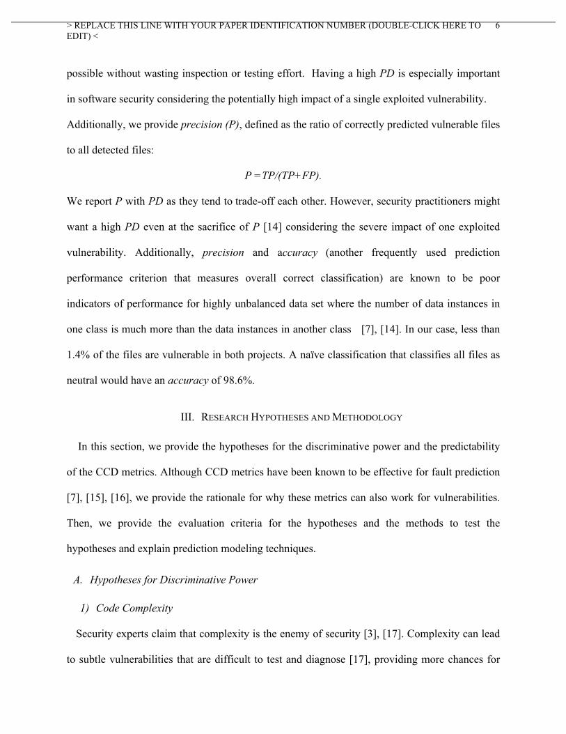
III. RESEARCH HYPOTHESES AND METHODOLOGY

In this section, we provide the hypotheses for the discriminative power and the predictability

of the CCD metrics. Although CCD metrics have been known to be effective for fault prediction

[7], [15], [16], we provide the rationale for why these metrics can also work for vulnerabilities.

Then, we provide the evaluation criteria for the hypotheses and the methods to test the

hypotheses and explain prediction modeling techniques.

A. Hypotheses for Discriminative Power

1) Code Complexity

Security experts claim that complexity is the enemy of security [3], [17]. Complexity can lead

to subtle vulnerabilities that are difficult to test and diagnose [17], providing more chances for


7

attackers to exploit. Complex code is difficult to understand, maintain, and test [18]. Therefore,

complex code would have a higher chance of having faults than simple code. Since attackers

exploit the faults in a program, complex code would be more vulnerable than simple code. From

this reasoning, we set up the following hypothesis on code complexity:

HIntraComplexity_D: Vulnerable files have a higher intra-file complexity than neutral files.

Highly coupled code has a higher chance of having input from external sources that are

difficult to trace where the input came from. Moreover, developers can use interfaces to

modules implemented by other developers or by a third party without properly understanding the

security concerns or assumptions of the modules. Therefore:

HCoupling_D: Vulnerable files have a higher coupling than neutral files.

Communication by comments between developers is important especially in open source

projects for which many developers can contribute on the same code segment without central

control. Novice developers who do not understand security concerns and do not follow secure

coding practice might comment less often. Furthermore, code developed in a hurry (perhaps

directly prior to release) might have fewer comments and be more vulnerable. Therefore:

HComments_D: Vulnerable files have a lower comment density than neutral files.

Table I defines the complexity metrics we use in this study. Each individual metric has the

same hypotheses defined as the same way as the hypotheses for its group. For example,

CountLineCode has the same hypotheses as HIntraComplexity_D.

1) Code Churn

Code is constantly evolving throughout the development process. Each new change in the

system brings a new risk of introducing a vulnerability [15], [19]. Therefore:

HCodeChurn_D: Vulnerable files have a higher code churn than neutral files.


8

Code churn can be counted in terms of the number of check-ins into a version control system

and the number of lines that have been added or deleted by code change. Specifically we break

down hypothesis HCodeChurn_D into the following two hypotheses:

HNumChanges_D: Vulnerable files have more frequent check-ins than neutral files.

HChurnAmount_D: Vulnerable files have more lines of code that have been changed than neutral

files.

Table II defines the code churn metrics that we use in this study.

TABLE II DEFINITIONS OF CODE CHURN METRICS

Related Hypothesis Metric Definition NumChanges The number of check-ins for a file since the creation of a file LinesChanged The cumulated number of code lines changed since the creation of a file

HCodeChurn_D

LinesNew The cumulated number of new code lines since the creation of a file

2) Developer Activity

Software development is performed by development teams working together on a common

project. Lack of team cohesion, miscommunications, or misguided effort can all result in security

problems [3]. Version control data can be used to construct a developer network and a

TABLE I DEFINITIONS OF COMPLEXITY METRICS

Related Hypothesis Metric Definition CountLineCode The number of lines of code in a file CountDeclFunction The number of functions defined in a file CountLineCodeDecl The number of lines of code in a file devoted to declarations CountLinePreprocessor The number of lines of code in a file devoted to preprocessing SumEssential The sum of essential complexity, where essential complexity is defined as the

number of branches after reducing all the programming primitives such as a for loop in a function’s control flow graph into a node iteratively until the graph cannot be reduced any further. Completely well-structured code has essential complexity 1 [18], [20]

SumCyclomaticStrict The sum of the strict cyclomatic complexity, where strict cyclomatic complexity is defined as the number of conditional statements in a function

SumMaxNesting The sum of the MaxNesting in a file, where MaxNesting is defined as the maximum nesting level of control constructs such as if or while statements in a function

MaxCyclomaticStrict The maximum of strict cyclomatic complexity in a file

HIntraComplexity_D

MaxMaxNesting The maximum of MaxNesting in a file SumFanIn The sum of FanIn, where FanIn is defined as the number of inputs to a function

such as parameters and global variables SumFanOut The sum of FanOut, where FanOut is defined as the number of assignment to the

parameters to call a function or global variables MaxFanIn The maximum of FanIn

HCoupling_D

MaxFanOut The maximum of FanOut HComments_D CommentDensity The ratio of lines of comments to lines of code


9

contribution network based upon “which developer(s) worked on which file,” using network

analysis as defined in Section II.

3.1) Developer Network Centrality

In our developer network, two developers are connected if they have both made a change to at

least one file in common during the period of time under study. The result is an undirected,

unweighted, and simple graph where each node represents a developer and edges are based on

whether or not they have worked on the same file during the same release. Central developers,

measured by a high degree, high betweenness, and low closeness, are developers that are well-

connected to other developers relative to the entire group. Refer to [16] for a more in-depth

example of how centrality metrics are derived from developer networks. A central developer

would likely have a better understanding of the group’s secure coding practices because of

his/her connections to the other developers of the team. Therefore:

HDeveloperCentrality_D: Vulnerable files are more likely to have been worked on by non-central

developers than neutral files.

The metrics we used for our hypotheses are shown in Table III. Note that we chose to not

study DNMaxDegree, DNMinCloseness, and DNMaxBetweenness because, for example, a high

DNMaxDegree means at least one central developer worked on the file, which is not as helpful

as knowing that high DNMinDegree denotes that all developers who worked on a file were

central. Note also that a high turnover rate in a project results in many non-central developers:

when new developers are added to the project, they initially lack connections to the other

developers.


10

TABLE III MEANING OF DEVELOPER ACTIVITY METRICS

Related Hypothesis Metric Problematic When

Meaning

DNMinDegree Low DNAvgDegree Low DNMaxCloseness High DNAvgCloseness High DNMinBetweenness Low

HDeveloperCentrality_D

DNAvgBetweenness Low

File was changed by developers who are not central to the network

DNMaxEdgeBetweenness High HDeveloperCluster_D DNAvgEdgeBetweenness High

File was contributed to by more than one cluster of developers, with few other files being worked on by each cluster

NumDevs High File was changed by many developers CNCloseness High HContributionCentrality_D CNBetweenness High

File was changed by developers who focused on many other files

3.2) Developer Network Cluster

Metrics of developer centrality give us information about individual developers, but we also

consider the relationship between groups of developers. In our developer network, a file that is

between two clusters was worked on by two groups of developers, and those two groups did

have many other connections in common. Clusters with a common connection, but few other

connections, may not be communicating about improving the security of the code they have in

common. Therefore:

HDeveloperCluster_D: Vulnerable files are more likely to be changed by multiple, separate

developer clusters than neutral files.

Since edges and files have a many-to-many relationship, we use the average and maximum of

edge betweenness on the developer network as provided in Table III.

3.3) Contribution Network

A contribution network [21] is a quantification of the focus made on the relationship between a

file and developers instead of relationship between developers as in developer networks. The

contribution network uses an undirected, weighted, and bipartite graph with two types of nodes:

developers and files. An edge exists where a developer made changes to a file, where the weight


11

is equal to the number of check-ins that developer made to the file. If a file has high centrality,

then that file was changed by many developers who made changes to many other files – referred

to as an “unfocused contribution.” [21] Files with an unfocused contribution would not get the

attention required to prevent the injection of vulnerabilities. Therefore:

HContributionCentrality_D: Vulnerable files are more likely to have an unfocused contribution than

neutral files.

Note that developers with high centrality can work with many people, but still work on one

small part of the system. Being a central developer means being central in terms of people and

not necessarily central in terms of the system. Contribution networks, on the other hand, are

structured around the system.

Table III provides the meaning of the contribution network metrics.

B. Evaluation of Hypotheses for Discriminative Power

To evaluate the discriminative power of the metrics, we test the null hypothesis that the means

of the metric for neutral files and vulnerable files are equal. Since our data set are skewed and

have unequal variance (See Fig. 3 in Section IV), we used the Welch’s t-test [22]. The Welch t-

test is a modified t-test to compare the means of two samples and is known to provide good

performance for skewed distributions with unequal variance. To see the association direction (i.e.

positively or negatively correlated), we compared the means and medians of the measures of

CCD metrics for the vulnerable and neutral files. Our hypotheses for discriminative power are

considered to be supported when the results from the Welch’s tests are statistically significant at

the p<0.05 level (p<0.0018 with a Bonferroni correction for 28 hypotheses tests) and when the

associations are in the direction prescribed in the hypotheses defined Section III.A. In addition to

the significance, we present the magnitude of the differences in measures between vulnerable


12

files and neutral files for representative metrics using boxplots.

C. Evaluation of Hypotheses for Predictability

We hypothesize that a subset of CCD metrics can predict vulnerable files at reasonable

prediction performance, specifically 70% PD and 25% PF. Since there are no universally

applicable standards for the threshold of high prediction performance, we use these average

values found from the fault prediction literature [7], [23], acknowledging that desirable level of

PD and PF depends on varying domains and business goals. We hypothesize that:

HComplexity_P: A model with a subset of complexity metrics can predict vulnerable files.

HCodeChurn_P: A model with a subset of code churn metrics can predict vulnerable files.

HDeveloper_P: A model with a subset of developer activity metrics can predict vulnerable files.

HCCD_P: A model with a subset of combined CCD metrics can predict vulnerable files.

Note that we select the subset of the metrics using the information gain ranking method instead

of testing every subset of the metrics (see Section III. E) because prediction performance from a

few selected metrics are known to be as good as using a large number of metrics [7].

Additionally we investigate whether the individual metrics can predict vulnerable files.

QIndividual_P: Can a model with individual CCD metric predict vulnerable files?

D. Measuring Inspection Reduction

Practitioners must consider how effective the prediction model is in reducing the effort for

code inspection even when reasonable PD and PF are achieved. Even though we use PD and PF

as the criteria to test our hypotheses on predictability, we further investigate the amount of

inspection and reduction in inspection by using the CCD metrics, which is related to cost and

effort, to describe the practicality of using CCD metrics. We use the number of files and the lines

of code to inspect as partial and relative estimators of the inspection effort. Such measures have


13

been used as cost estimators in prior studies [24], [25]. In our definition, overall inspection is

reduced if the percentage of lines of code or the percentage of files to inspect is smaller than the

percentage of faults identified in those files [24], [25]. For example, if we randomly choose files

to inspect, we need to inspect 80% of the total files to obtain 80% PD. If a prediction model

provides 80% PD with less than 80% of the total files, the model reduced the cost for inspections

compared to a random file selection. The two cost measurements are formally defined as below:

File Inspection (FI) ratio is the ratio of files predicted as vulnerable (that is, the number of files

to inspect) to the total number of files for the reported PD:

FI = (TP+FP) / (TP+TN+FP+FN).

For example, PD=80% and FI=20% mean that within the 20% of files inspected based on the

prediction results, 80% of vulnerable files can be found.

LOC Inspection (LI) ratio is the ratio of lines of code to inspect to the total lines of code for

the predicted vulnerabilities. First, we define lines of code in the files that were true positives, as

TPLOC, similarly with TNLOC, FPLOC, and FNLOC. Then LI is defined as below:

LI = TPLOC+FPLOC / (TPLOC+TNLOC+FPLOC+FNLOC).

While FI and LI estimate how much effort is involved, we need measures to provide how

much effort is reduced. We define two cost-reduction measurements.

File Inspection Reduction (FIR) is the ratio of the reduced number of files to inspect by using

the model with CCD metrics compared to a random selection to achieve the same PD.

FIR = (PD – FI) / PD.

LOC Inspection Reduction (LIR) is the ratio of reduced lines of code to inspect by using a

prediction model compared to a random selection to achieve the same PV.

LIR = (PV – LI) / PV


14

where PV is defined as below.

Predicted Vulnerability (PV) ratio is the ratio of the number of vulnerabilities in the files

predicted as vulnerable to the total number of vulnerabilities. First, we define the number of

vulnerabilities in the files that were true positives, as TPVuln, similarly with TNVuln, FPVuln, and

FNVuln. Then PV is defined as below:

PV = TPVuln / (TPVuln+ FNVuln).

E. Prediction Models and Experimental Design

We used Logistic regression to predict vulnerable files. Logistic regression computes the

probability of occurrence of an outcome event from given independent variables by mapping the

linear combination of independent variables to the probability of outcome using the log of odds

ratio (logit). A file is classified as vulnerable when the outcome probability is greater than 0.5.

We also tried other four classification techniques including J48 decision tree [26], Random

forest [27], Naïve Bayes [26], and Bayesian network [26] that have been effective for fault

prediction. Among those, J48, Random forest, and Bayesian network provided similar results to

Logistic regression, while Naïve Bayes provided higher PD with higher FI than other techniques.

Lessmann et al. also reported that no significant difference in prediction performance was found

between the 17 classification techniques they investigated [28]. Therefore, we only present the

results from Logistic regression in this paper.

To validate a model’s predictability, we performed next-release validation for Mozilla Firefox

where we had 34 releases and 10x10 cross-validation [26] for the RHEL4 kernel where we only

had a single release. For next-release validation, data from the most recent three previous

releases were used to train against the next release (i.e. train on releases R-3 to R-1 to test against

release R). Using only recent releases was to accommodate for process change, technology


15

change, and developer turnovers. For 10x10 cross-validation, we randomly split the data set into

ten folds and used one fold for testing and the remaining folds for training, rotating each fold as

the test fold. Each fold was stratified to properly distribute vulnerable files to both training and

test data set. The entire process was then repeated ten times to account for possible sampling bias

in random splits. Overall, 100 predictions were performed for 10x10 cross-validation and the

results were averaged.

Using many metrics in a model does not always improve the prediction performance since

metrics can provide redundant information [7]. We found this issue to be the case in our study.

Therefore, we selected only three variables using two variable selection methods: the

information gain ranking method and the correlation-based greedy feature selection method [26].

Both methods provided similar prediction performance. However, the set of chosen variables by

the two selection methods were different. We present the results using the information gain

ranking method in this study.

We performed the prediction on both the raw and log transformed data. For Logistic regression,

PD was improved at the sacrifice of precision after log transformation. We present results using

log transformation in this paper.

Our data is heavily unbalanced between majority class (neutral files) and minority class

(vulnerable files). Prior studies have shown that the performance is improved (or at least not

degraded) by “balancing” the data [23], [29]. Balancing the data can be achieved by duplicating

the minority class data (over-sampling) or removing randomly chosen majority class data (under-

sampling) until the numbers of data instances in the majority class and the minority class become

equal [23]. We used under-sampling in this study since under-sampling provided better results

than using the unbalanced data and reduced the time for evaluation.


16

Figures 1 and 2 provide the pseudo code of our experimental design explained above for next-

release validation and cross-validation. The whole process of validation is repeated ten times to

account for possible sampling bias due to random removal of data instances. The ten times of

repetition also account for the bias due to random splits in cross-validation. In Figures 1 and 2,

performance represents the set of evaluation criteria, cost-reduction measurements, and their

relevant measurements defined in Section II.C and III.D. For next-release validation, the input is

three prior releases for training a model and one release for testing. For cross-validation, the

input is the whole data set.

next_release_validation (Set R1, Set R2, Set R3, Set R4) { Strain ← R1∪ R2 ∪ R3 Stest ← R4 performance ← 0 repeat 10 times {

Strain _ vulnerable ← vulnerable files in Strain N ← |Strain_ vulnerable| Strain_ neutral ← N neutral files remaining after random removal from Strain for under-sampling

Strain ← Strain_ vulnerable ∪ Strain_ neutral V ← select variables using the InfoGain variable selection method from Strain Train the model M on Strain and variables V performance ← performance + prediction performance of M tested on Stest

} return performance ← performance / 10 }

Fig. 1. Pseudo code for next-release-validation

cross_validation (Set R) { performance ← 0

repeat 10 times { Randomly split R into 10 stratified bins, B = {b1, b2, …, b10} for each bin bi {

Strain ←B – { bi } Stest ← bi Strain_vulnerable← vulnerable files in Strain N ← |Strain_vulnerable| Strain_neutral ← N neutral files remaining after random removal from Strain for under-sampling

Strain ←Strain_ vulnerable ∪ Strain_ neutral V ← select variables using the InfoGain selection method from Strain Train the model M on Strain and variables V performance ← performance + prediction performance of M tested on Stest

} } return performance ← performance / 100

} Fig. 2. Pseudo code for cross-validation


17

We used the Weka 3.74 with default options for prediction models and variable selection

except for limiting the number of variables to be selected to three for multivariate predictions.

IV. CASE STUDY 1: MOZILLA FIREFOX

Our first case study is Mozilla Firefox, a widely-used open source web browser. Mozilla

Firefox had 34 releases at the time of data collection developed over four years. Each release

consists of over 10,000 files and over two million lines of source code.

A. Data Collection

To measure the number vulnerabilities fixed in a file, we counted the number of bug reports

that include the details on vulnerabilities and on how the vulnerabilities have been fixed for the

file. We collected vulnerability information from Mozilla Foundation Security Advisories

(MFSAs) 5. Each MFSA includes bug ids that are linked to the Bugzilla6 bug tracking system.

Mozilla developers also add bug ids to the log of the CVS version control system7 when they

check in files to the CVS after the vulnerabilities have been fixed. We searched the bug ids from

the CVS log to find the files that have been changed to fix vulnerabilities, similar to the approach

found in other studies [30]. The number of MFSAs for Firefox was 197 as of 2 August, 2008.

The vulnerability fixes for the MFSAs were reported in 560 bug reports. Among them, 468 bug

ids were identified from the CVS log. Although some of the files were fixed for regression, all

those files were also fixed for vulnerabilities. Therefore, we counted those files as vulnerable.

To collect complexity metrics, we used Understand C++8, a commercial metrics collection

tool. We limited our analysis to C/C++ and their header files to obtain complexity metrics,

4 http://www.cs.waikato.ac.nz/ml/weka 5 http://www.mozilla.org/security/announce/ 6 http://www.bugzilla.org/ 7 https://developer.mozilla.org/en/Mozilla_Source_Code_Via_CVS 8 http://www.scitools.com


18

excluding other files types such as script files and make files. We obtained code churn and

developer activity metrics from the CVS version control system.

At the time of data collection, Firefox 1.0 and Firefox 2.0.0.16 were the first and the last

releases that had vulnerability reports. The gap between Firefox releases ranged from one to two

months. Since each release had only a few vulnerabilities (not enough to perform analysis at each

Firefox release), we combined the number of vulnerabilities for three consecutive releases, and

will refer to those releases as a combined release, denoted by R1 through R11 in this paper. For

each release, we used the most recent three combined releases (RN-3 to RN-1) to predict

vulnerable files in RN. We collected metrics for 11 combined releases. Table IV provides the

project statistics for the combined 11 releases.

TABLE IV PROJECT STATISTICS FOR MOZILLA FIREFOX

No. Firefox Release # of Files LOC Mean LOC Files with Vulns.

Total Vulns.

Vulns. per File

% of Files with Vulns.

R1 1.0 / 1.0.1 / 1.0.2 10,320 2,060,908 200 70 84 0.008 0.678 R2 1.0.3 / 1.0.4 / 1.0.5 / 1.0.69 10,321 2,063,960 200 123 134 0.013 1.192 R3 1.0.7 / 1.5 / 1.5.0.1 10,321 2,064,747 200 93 159 0.015 0.901 R4 1.5.0.2 / 1.5.0.3 / 1.5.0.4 10,956 2,226,540 203 100 138 0.013 0.913 R5 1.5.0.5 / 1.5.0.6 / 1.5.0.7 10,961 2,230,313 204 109 153 0.014 0.994 R6 1.5.0.8 / 2.0 / 2.0.0.1 10,961 2,232,890 204 87 124 0.011 0.794 R7 2.0.0.2 / 2.0.0.3 / 2.0.0.4 11,060 2,294,287 207 114 162 0.015 1.031 R8 2.0.0.5 / 2.0.0.6 / 2.0.0.7 11,060 2,299,054 208 55 72 0.007 0.497 R9 2.0.0.8 / 2.0.0.9 / 2.0.0.10 11,076 2,301,398 208 14 15 0.001 0.126 R10 2.0.0.11 / 2.0.0.12 / 2.0.0.13 11,077 2,301,832 208 84 110 0.010 0.758 R11 2.0.0.14 / 2.0.0.15 / 2.0.0.16 11,080 2,304,048 208 27 46 0.004 0.244

B. Discriminative Power Test and Univariate Prediction Results

Table V shows the results of hypotheses testing for discriminative power and the univariate

prediction using Logistic regression for individual metrics from release R4, the first test data set

that uses the most three recent releases to train a prediction model. In Table V, the plus sign in

the Association column indicates that the vulnerable files had a higher measure than neutral files.

DNAvgDegree was the only sign that did not completely agree with its hypothesis. We discuss

the reason in Section VI. 27 of the 28 metrics showed a statistically significant difference

9 The vulnerabilities for Firefox 1.0.5 and Firefox 1.0.6 were reported together. Therefore, we considered those two versions as one version.


19

between vulnerable and neutral files using the Welch’s t-test after a Bonferroni correction as

shown in Table V. We also compared the mean and median of each measurement for vulnerable

and neutral files to find the association direction (positive or negative). Fig. 3 shows the boxplots

of comparisons of log scaled measures between vulnerable and neutral files for the three

representative metrics from each type of CCD metrics: CountLineCode, NumChanges, and

NumDevs. The medians of the three metrics for the vulnerable files were higher than the ones for

the neutral files, as we hypothesized.

Fig. 3. Comparison of measures for vulnerable and neutral files

In Table V, the means of PD and PF are averaged over ten repetitions of predictions for R4

according to the algorithm provided in Fig. 1 and presented with standard deviations. We test

whether individual metrics can predict vulnerable files at over 70% PD with less than 25% PF as

described in Section III.C. N(QP) represent the number of predictions that satisfy our criteria in

the 80 predictions (ten repetitions for each of the eight combined releases). NumChanges and

CNCloseness satisfied our criteria in all 80 predictions. CountLineCodeDecl, LinesChanged, and

NumDevs satisfied our criteria in over half of the predictions. Most metrics provided very small

variations between predictions except for CommentDensity, Linesnew, and DNMinBetweenness.

Note that we provide N(Qp) instead of averaging the prediction results across all releases because

averaging the results for different data sets can mislead the interpretation of the results from each

data set [31].


20

TABLE V RESULTS OF DISCRIMINATIVE POWER TEST AND UNIVARIATE PREDICTION MOZILLA FIREFOX

Discriminative Power Predictability Mean for R4 Std. for R4

Related Hypothesis Metric Welch-t Association

HD* PD* PF* QP* PD PF N(QP)*

Complexity CountLineCode √ + √ 82 28 X 0.4 0.9 1 CountDeclFunction √ + √ 87 68 X 0.0 0.0 0 CountLineCodeDecl √ + √ 79 25 √ 0.0 0.8 47 CountLinePreprocessor √ + √ 76 26 X 0.9 0.9 0 SumEssential √ + √ 86 60 X 0.3 3.0 0 SumCyclomaticStrict √ + √ 86 60 X 0.0 1.2 0 MaxCyclomaticStrict √ + √ 87 68 X 0.0 0.0 0 SumMaxNesting √ + √ 82 53 X 0.0 0.0 0

HIntraComplexity_D

MaxMaxNesting √ + √ 82 53 X 0.0 0.0 0 SumFanIn √ + √ 87 57 X 0.0 0.0 0 SumFanOut √ + √ 86 62 X 0.0 0.0 0 MaxFanIn √ + √ 87 57 X 0.0 0.0 0 HCoupling_D MaxFanOut √ + √ 86 62 X 0.0 0.0 0

HComments_D CommentDensity X – X 59 45 X 15.4 21.8 0 Code Churn HNumChanges_D NumChanges √ + √ 86 23 √ 0.8 1.2 80

LinesChanged √ + √ 85 25 √ 0.3 1.4 76 HChurnAmount_D LinesNew √ + √ 88 58 X 0.9 9.1 0 Developer Activity

DNMinDegree √ – √ 74 84 X 4.2 1.0 0 DNAvgDegree √ + X 98 77 X 0.0 0.9 0 DNMaxCloseness √ + √ 100 95 X 0.0 0.1 0 DNAvgCloseness √ + √ 100 95 X 0.0 0.0 0 DNMinBetweenness √ – √ 53 45 X 0.5 30.7 0


DNAvgBetweenness √ – √ 99 87 X 0.3 0.8 0 DNMaxEdgeBetweenness √ + √ 88 30 X 0.0 0.0 0 HDeveloperCluster_D DNAvgEdgeBetweenness √ + √ 88 30 X 0.0 0.0 0 NumDevs √ + √ 84 24 √ 1.5 1.6 58 CNCloseness √ + √ 82 22 √ 0.0 0.0 80 HContributionCentrality_D CNBetweenness √ + √ 64 9 X 0.0 0.0 20

*. HD: Hypothesis test for discriminative power, PD: Probability of detection, PF: Probability of false alarm, QP: Question for predictability, N(QP): Number of predictions that provided over 70% PD with less than 25% PF from 80 predictions

Note that a single metric can provide such a high PD and a low PF. We further investigate the

predictability of CCD metrics when they are used together in a model in the following subsection.

C. Multivariate Prediction Results

Although metrics can have low predictability individually, combining metrics into a model

can result in better predictability [32]. Therefore, we created four types of models using

complexity, code churn, developer activity, and combination of the CCD metrics. From each set

of the metrics, three variables were selected as we explained in Section III.E.

Fig. 4 shows PD, PF, FI, LI, FIR, and LIR across releases where the results from each release

were averaged over the results from the ten repetitions of next-release validation using Logistic


21

regression. All the models with code churn, developer activity, and combined CCD metrics

provided similar results across releases; PD was between 68% to 88%% and PF was between

17% to 26%; File Inspection Ratio (FI) was between 17% to 26% resulting in 66% to 80%

reduction in the files to inspect; Line Inspection Ratio (LI) was between 49% to 65% resulting in

16% to 42% of reduction in lines of code to inspect. The models using complexity metrics

provided 76% to 86% PD and 22% to 34% PF. FI for the models using complexity metrics was

between 22% to 34% resulting in 61% to 72% reduction in file inspection. LI for the models

using complexity metrics was much higher than LI for the other models (74% to 85%) resulting

in only 7% reduction in code inspection at best. In the worst case, 3% more code required to

inspect than the percentage of lines of code chosen by random selection. Note that PF and FI

showed almost identical performance for all models. We discuss the similarity between PF and

FI in Section VI.

The three types of models generally provided consistent PD except for R5 and R10. The

models using complexity metrics provided lower PD than other models, but provided consistent

results even in R5 and R10. Instead, PF from the models using complexity metrics suddenly

increased in R10. We conjecture the reason of the sudden decrease in performance for R10 is

because the number of vulnerable files in R10 suddenly increases when the model was trained

with recent two releases (R8 and R9) with relatively few vulnerabilities, and the model trained

from the past trend did not work properly. However, we were not able to find out any particular

reason of the sudden decreases in performance for R5. All the prediction results from the three

types of models gradually improved as the system matures, but the results from models using

complexity metrics stayed constant or degraded.


22

Fig. 4. Prediction results for Mozilla Firefox across releases

Table VI provides detailed results for release R4 including standard deviations. The models

with code churn metrics and combined CCD metrics satisfied our prediction criteria in over 90%

of predictions out of 80 predictions (ten repetitions for each of the eight combined releases). All

of the models satisfied our criteria in over 50% of the 80 predictions. Standard deviations in PD

and PF were less than 3 in all models for release R4. Interestingly, no multivariate models were

noticeably better than some of the best univariate models.


23

TABLE VI RESULTS OF MULTIVARIATE PREDICTION FOR MOZILLA FIREFOX

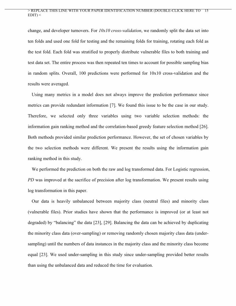
Predictability for R4 Inspection Costs for R4 Mean Standard Dev. Costs Cost Reduction PD PF P PD PF N(HP) PV FI LI FIR LIR

Complexity 79 25 3 0.7 0.8 40 84 26 79 68 6 Code churn 84 23 3 1.2 1.3 76 88 23 59 72 33 Developer activity 85 26 3 1.7 2.8 62 88 26 59 69 34 Combined CCD 85 24 3 1.8 1.7 74 89 24 61 72 31

The amount of files to inspect reduced by 68% to 72% depending on the models for R4. The

amount of lines of code to inspect reduced by 31% to 34% with code churn, developer activity,

and combined CCD metrics, and only 6% with complexity metrics for release R4.

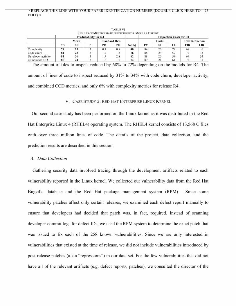
V. CASE STUDY 2: RED HAT ENTERPRISE LINUX KERNEL

Our second case study has been performed on the Linux kernel as it was distributed in the Red

Hat Enterprise Linux 4 (RHEL4) operating system. The RHEL4 kernel consists of 13,568 C files

with over three million lines of code. The details of the project, data collection, and the

prediction results are described in this section.

A. Data Collection

Gathering security data involved tracing through the development artifacts related to each

vulnerability reported in the Linux kernel. We collected our vulnerability data from the Red Hat

Bugzilla database and the Red Hat package management system (RPM). Since some

vulnerability patches affect only certain releases, we examined each defect report manually to

ensure that developers had decided that patch was, in fact, required. Instead of scanning

developer commit logs for defect IDs, we used the RPM system to determine the exact patch that

was issued to fix each of the 258 known vulnerabilities. Since we are only interested in

vulnerabilities that existed at the time of release, we did not include vulnerabilities introduced by

post-release patches (a.k.a “regressions”) in our data set. For the few vulnerabilities that did not

have all of the relevant artifacts (e.g. defect reports, patches), we consulted the director of the


24

RHSR team to correct the data and the artifacts. We collected vulnerabilities reported from

February 2005 through July 2008.

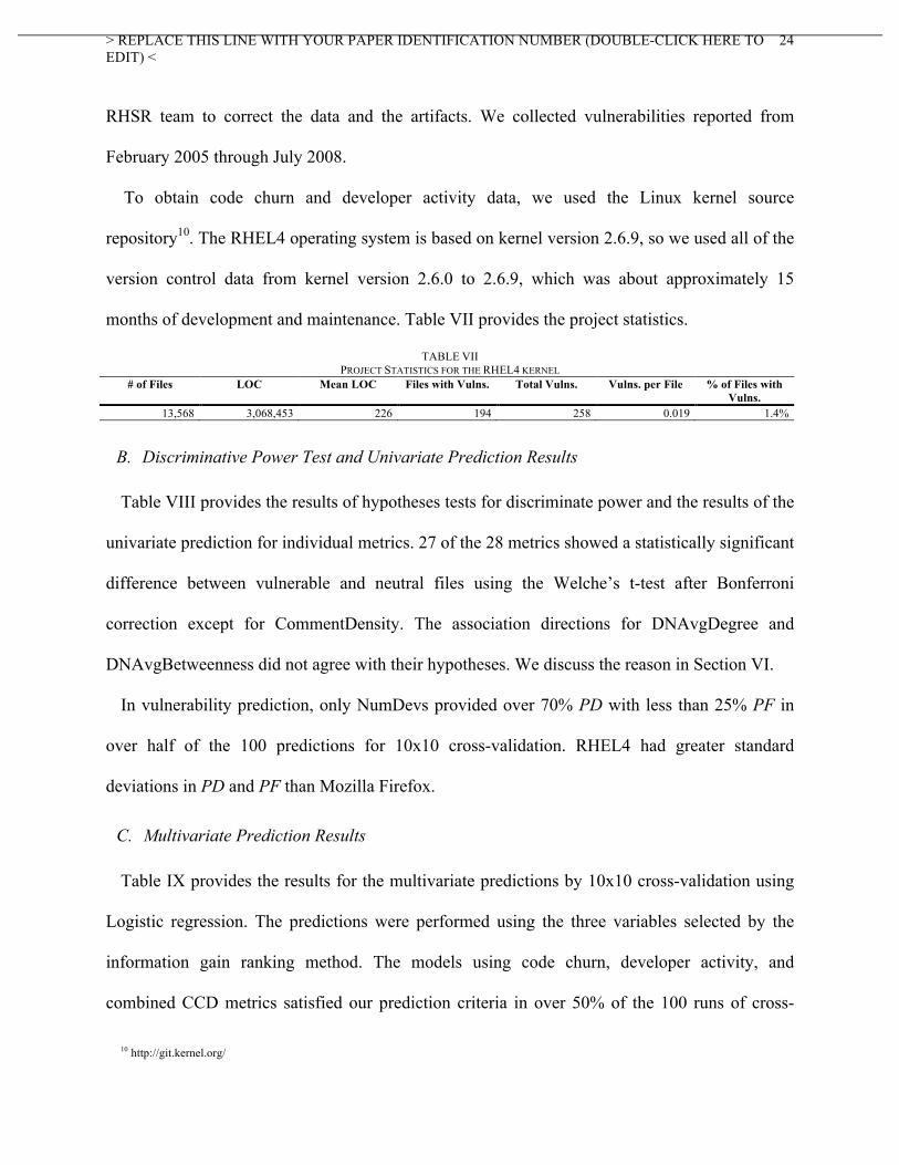
To obtain code churn and developer activity data, we used the Linux kernel source

repository10. The RHEL4 operating system is based on kernel version 2.6.9, so we used all of the

version control data from kernel version 2.6.0 to 2.6.9, which was about approximately 15

months of development and maintenance. Table VII provides the project statistics.

TABLE VII PROJECT STATISTICS FOR THE RHEL4 KERNEL

# of Files LOC Mean LOC Files with Vulns. Total Vulns. Vulns. per File % of Files with Vulns.

13,568 3,068,453 226 194 258 0.019 1.4%

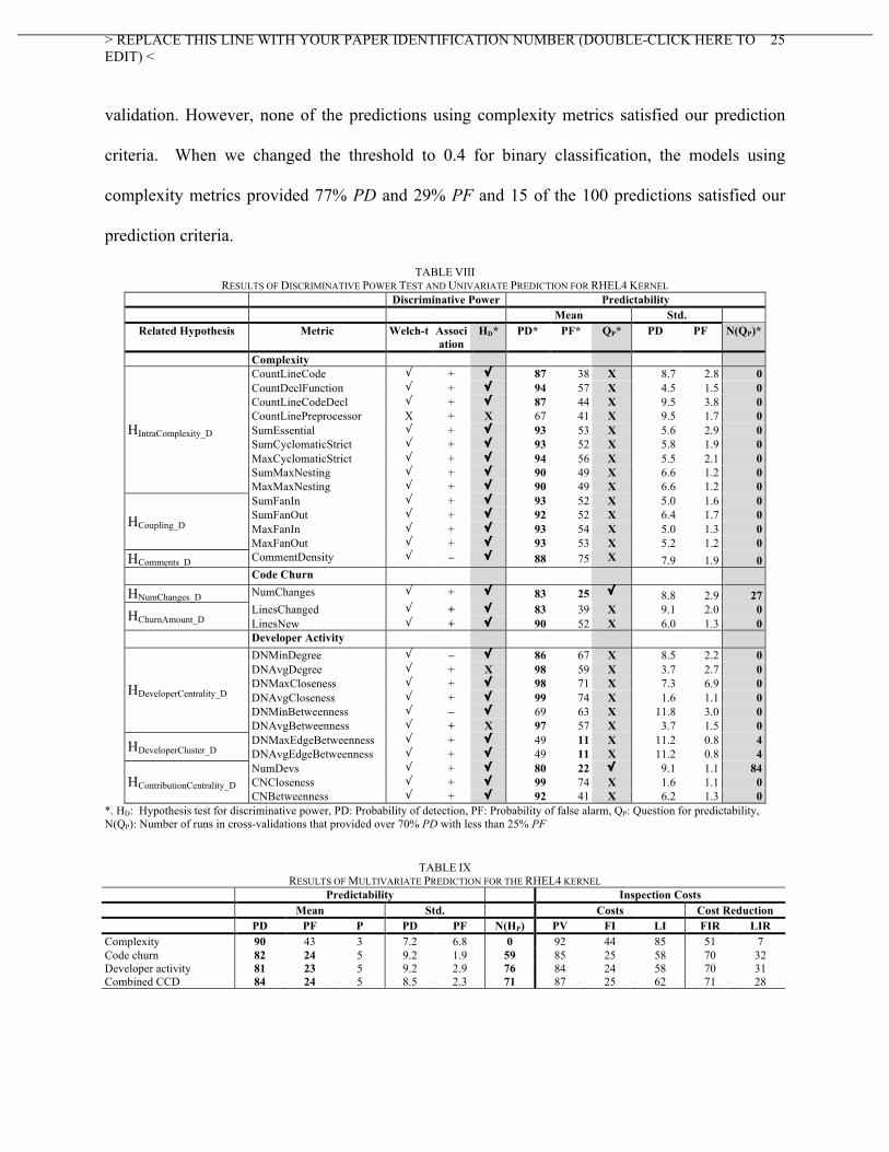
B. Discriminative Power Test and Univariate Prediction Results

Table VIII provides the results of hypotheses tests for discriminate power and the results of the

univariate prediction for individual metrics. 27 of the 28 metrics showed a statistically significant

difference between vulnerable and neutral files using the Welche’s t-test after Bonferroni

correction except for CommentDensity. The association directions for DNAvgDegree and

DNAvgBetweenness did not agree with their hypotheses. We discuss the reason in Section VI.

In vulnerability prediction, only NumDevs provided over 70% PD with less than 25% PF in

over half of the 100 predictions for 10x10 cross-validation. RHEL4 had greater standard

deviations in PD and PF than Mozilla Firefox.

C. Multivariate Prediction Results

Table IX provides the results for the multivariate predictions by 10x10 cross-validation using

Logistic regression. The predictions were performed using the three variables selected by the

information gain ranking method. The models using code churn, developer activity, and

combined CCD metrics satisfied our prediction criteria in over 50% of the 100 runs of cross-

10 http://git.kernel.org/


25

validation. However, none of the predictions using complexity metrics satisfied our prediction

criteria. When we changed the threshold to 0.4 for binary classification, the models using

complexity metrics provided 77% PD and 29% PF and 15 of the 100 predictions satisfied our

prediction criteria.

TABLE VIII RESULTS OF DISCRIMINATIVE POWER TEST AND UNIVARIATE PREDICTION FOR RHEL4 KERNEL

Discriminative Power Predictability Mean Std.

Related Hypothesis Metric Welch-t Association

HD* PD* PF* QP* PD PF N(QP)*

Complexity CountLineCode √ + √ 87 38 X 8.7 2.8 0 CountDeclFunction √ + √ 94 57 X 4.5 1.5 0 CountLineCodeDecl √ + √ 87 44 X 9.5 3.8 0 CountLinePreprocessor X + X 67 41 X 9.5 1.7 0 SumEssential √ + √ 93 53 X 5.6 2.9 0 SumCyclomaticStrict √ + √ 93 52 X 5.8 1.9 0 MaxCyclomaticStrict √ + √ 94 56 X 5.5 2.1 0 SumMaxNesting √ + √ 90 49 X 6.6 1.2 0

HIntraComplexity_D

MaxMaxNesting √ + √ 90 49 X 6.6 1.2 0 SumFanIn √ + √ 93 52 X 5.0 1.6 0 SumFanOut √ + √ 92 52 X 6.4 1.7 0 MaxFanIn √ + √ 93 54 X 5.0 1.3 0 HCoupling_D MaxFanOut √ + √ 93 53 X 5.2 1.2 0

HComments_D CommentDensity √ – √ 88 75 X 7.9 1.9 0 Code Churn

HNumChanges_D NumChanges √ + √ 83 25 √ 8.8 2.9 27 LinesChanged √ + √ 83 39 X 9.1 2.0 0 HChurnAmount_D LinesNew √ + √ 90 52 X 6.0 1.3 0

Developer Activity DNMinDegree √ – √ 86 67 X 8.5 2.2 0 DNAvgDegree √ + X 98 59 X 3.7 2.7 0 DNMaxCloseness √ + √ 98 71 X 7.3 6.9 0 DNAvgCloseness √ + √ 99 74 X 1.6 1.1 0 DNMinBetweenness √ – √ 69 63 X 11.8 3.0 0


DNAvgBetweenness √ + X 97 57 X 3.7 1.5 0 DNMaxEdgeBetweenness √ + √ 49 11 X 11.2 0.8 4 HDeveloperCluster_D DNAvgEdgeBetweenness √ + √ 49 11 X 11.2 0.8 4 NumDevs √ + √ 80 22 √ 9.1 1.1 84 CNCloseness √ + √ 99 74 X 1.6 1.1 0 HContributionCentrality_D CNBetweenness √ + √ 92 41 X 6.2 1.3 0

*. HD: Hypothesis test for discriminative power, PD: Probability of detection, PF: Probability of false alarm, QP: Question for predictability, N(QP): Number of runs in cross-validations that provided over 70% PD with less than 25% PF

TABLE IX

RESULTS OF MULTIVARIATE PREDICTION FOR THE RHEL4 KERNEL Predictability Inspection Costs Mean Std. Costs Cost Reduction PD PF P PD PF N(HP) PV FI LI FIR LIR

Complexity 90 43 3 7.2 6.8 0 92 44 85 51 7 Code churn 82 24 5 9.2 1.9 59 85 25 58 70 32 Developer activity 81 23 5 9.2 2.9 76 84 24 58 70 31 Combined CCD 84 24 5 8.5 2.3 71 87 25 62 71 28


26

The reduction in file inspection compared to a random file selection was between 51% and

71%. The reduction in lines of code inspection was over 28% for code churn, developer activity,

and combined CCD metrics and only 7% for complexity metrics.

VI. SUMMARY OF TWO CASE STUDIES AND DISCUSSION

Table X provides the summary of our hypotheses testing. The hypotheses for discriminative

power were supported by at least 24 of the 28 metrics for both projects except for

CommentDensity and DNAvgDegree for Firefox, and CountLinePreprocessor, DNAvgDegree,

and DNAvgBetweenness for RHEL 4. Among these, CountLinePreprocessor and

CommentDensity were not discriminative of neutral and vulnerable files. DNAvgDegree and

DNAvgBetweenness disagreed with our hypotheses in the direction of association. While

DNMinDegree was negatively correlated with vulnerabilities and supported our hypothesis,

DNAvgDegree was positively correlated in both projects. This means that files are more likely to

be vulnerable if they are changed by developers who work on many other files with other

developers on average, but when all of the developers are central, the file is less likely to be

vulnerable. For DNAvgBetweeenness, we were not able to find any clear reason for the

hypothesis to not be supported.

Overall, 80 predictions were performed for the eight releases (R4 – R11) of Firefox with ten

repetitions to account for sampling bias and 100 predictions for RHEL 4 for 10x10 cross-

validation. In the univariate predictions, 5 of the 28 metrics supported the hypotheses in 50% of

the total predictions for Firefox and 1 of the 28 metrics for RHEL 4. Considering only the small

number of metrics satisfied the prediction criteria in univariate prediction, relying on a single

metric is a dangerous practice. In multivariate predictions, the models using code churn,

developer activity, and combined CCD metrics supported the hypotheses in over 50% of the total


27

predictions for both project. Even though the models using complexity metrics supported the

hypotheses in over 50% of the total predictions for Firefox, none of the predictions were

successful for RHEL 4. Considering this result together with the surprisingly low (even negative)

inspection cost reduction seen in Fig. 4 of Section IV, although whether lines of code is an

effective cost measurement depends on situation [25], the effectiveness of complexity metrics as

indicators of vulnerabilities is weak for the complexity metrics we collected.

TABLE X SUMMARY OF HYPOTHESES TESTING

Hypotheses Firefox RHEL 4

HComplexity_D Vulnerable files are more complex than neutral files. Yes for 13 of 14 metrics. Yes for 13 of 14 metrics.

HCodeChurn_D Vulnerable files have a higher code churn than neutral files. Yes for all 3 metrics. Yes for all 3 metrics.

HDeveloper_D Vulnerable files are more likely to have been changed by poor developer activity than neutral files.

Yes for 10 of 11 metrics.

Yes for 9 of 11 metrics.

QIndividual_P Can a model with individual CCD metric predict vulnerable files?* 5 of 28 metrics satisfied the prediction criteria in over half of the 80 predictions.

1 of 28 metrics satisfied the prediction criteria in over half of the 100 predictions.

HComplexity_P A model with a subset of complexity metrics can predict vulnerable files. *

Supported by 40 of 80 predictions.

Supported by 0 of 100 cross-validations.

HCodeChurn_P A model with a subset of code churn metrics can predict vulnerable files. *



HDeveloper_P A model with a subset of developer metrics can predict vulnerable files. *



HCCD_P A model with a subset of combined CCD metrics can predict vulnerable files. *



*. The criteria for the hypotheses tests for vulnerability prediction are 70 % PD and 25% PF.

Precision (P) from all the models for both projects was strikingly low with less than five as a

result of large numbers of false positives. This result is especially interesting because almost all

of the individual metrics had strong discriminative power according to Welch’s t-test. This

discrepancy can be explained from the boxplots in Fig.3 of Section IV where the mean values in

the individual metrics show clear difference, but the considerable numbers of neutral files are

still in the expected range of vulnerable files leading to a large number of false positives.

Organizations can improve P by raising the threshold for binary classification to reduce false

positives. However, PD can become lower in that case as PD and P tend to trade-off each other.


28

Whether a model that provides high PD and low P is better than a model that provides high P

and low PD is arguable. An organization may prefer to detect many vulnerabilities because they

have a large amount of security resources and security expertise. On the other hand, other

organizations may prefer a model that provides high P that reduces the waste of effort even with

low PD.

Preference for high PD and low P requires some caution in terms of cost-effectiveness. From

the results in Tables VI and IX, organizations are guided to inspect only less than 26% of files to

find over around 80% of vulnerable files in most models. However, since the projects have a

large amount of files, the number of files to inspect is still large. For example, Firefox release R4

has around 11,000 files and the model with combined CCD metrics provided 24% FI identifying

2,640 files to inspect. If security inspection requires one person-day per file, over seven full

years would be spent for one security engineer to inspect the 2,640 files. If the files to inspect are

reduced to 10% of the predicted files (264 files) by further manual prioritization, the overall

inspection would take essentially a year for one security engineer only to find a further reduced

set of vulnerabilities. In that case, pursuing high P and low PD might be a more cost-effective

approach than pursing high PD and low P. However, because the inspection time can greatly

vary depending on the ability and the number of security engineers involved, organizations

should use this illustration and our prediction results only to make an informed decision.

Among the metrics we investigated, history metrics such as code churn and developer activity

metrics provided higher prediction performance than the complexity. Therefore, historical

development information is a favorable source for metrics and using historical information is

recommended whenever possible. However, our result is limited to the metrics that we collected.

Other complexity metrics may provide better results.


29

We also observed sudden changes in prediction performance in a few releases of Firefox where

we used next-release validation. This result cannot be observed with cross-validation. Therefore,

our study reveals the importance of next-release validation to validate metrics for vulnerability

prediction whenever possible.

For both projects, PF and FI are almost equal. We believe the reason for this was that the

percentage of files with vulnerabilities is very low (< 1.4%) and P is also very low. The low

percentage of vulnerable files means that the total number of files (TP+TN+FP+FN) is almost

the same as the number of non-vulnerable files (FP+TN). The low P means that the number of

positive predictions (TP+FP) is very close to FP. Therefore, FI computed by

(TP+FP)/(TP+TN+FP+FN) and PF computed by FP/(FP+TN) are almost equal. Knowing this

fact provide us a useful hint to guess the number files to inspect when both the percentage of

vulnerable files and P are very low.

Interestingly, NumDevs was effective in the vulnerability prediction in our study while another

study [33] observed that NumDevs did not improve the prediction performance significantly.

The two major differences between the studies are (a) their study was closed-source and ours

was open-source; and (b) they were predicting faults and not vulnerabilities.

Further study on the difference in open- and closed-source projects and on the difference

between fault and vulnerability prediction may further improve our understanding on faults and

vulnerabilities on various types of projects and better guide code inspection and testing efforts.

In a preliminary study comparing fault prediction and vulnerability prediction for Firefox 2.0, we

trained a model for predicting vulnerabilities and a model for predicting faults, both using

complexity, code churn, and fault history metrics [34]. The fault prediction provided 18% lower

PD and 38% higher P than vulnerability prediction. The study also showed that the prediction


30

performance was largely affected by the number of reported faulty or vulnerable files. Since only

13% of faulty files were reported as vulnerable, further effort is required to characterize the

difference between faults and vulnerabilities and to find better way to predict vulnerable code

locations.

VII. THREATS TO VALIDITY

Since our data is based on known vulnerabilities, our analysis does not account for latent

(undiscovered) vulnerabilities. Additionally, only fixed vulnerabilities are publicly reported in

detail by organizations to avoid the possible attacks from malicious users; unfixed vulnerabilities

are usually not publicly available. However, considering the wide use of both projects, we

believe the currently-reported vulnerabilities are not too limited to jeopardize our results.

We combined every three releases and predicted vulnerabilities for next three releases for

Mozilla Firefox. Using this study design, the predictions will be performed on the every third

release. However, considering the short time periods between releases (one or two months), we

consider that the code and process history information between the three releases within a

combined release is relatively similar and those releases share many similar vulnerabilities. This

decision was made to increase the percentage of vulnerabilities in each release because the

percentage of vulnerabilities for the subject projects was too low to train the prediction models.

In fact, once enough training data is cumulated during a few initial releases, one could predict

vulnerabilities in actual releases rather than in combined releases. Alternatively, we could use

vulnerability history as a part of metrics together with CCD metrics as was used in [33] instead

of combining releases. We plan to extend our study to accommodate both of the approaches. For

Mozilla Firefox, not all of the bug ids for vulnerability fixes were identified from the CVS log,

which could lead to the lower prediction performance.


31

Actual security inspections and testing are not perfect, so our results are optimistic in

predicting exactly how many vulnerable files will be found by security inspection and testing.

As with all empirical studies, our results are limited to the two projects we studied. To

generalize our observations from this study to other projects in various languages, sizes,

domains, and development processes, further studies should be performed.

VIII. RELATED WORK

This section introduces prior studies on the software vulnerability prediction and usages of

CCD metrics in fault prediction.

A. Vulnerability Prediction

Neuhaus et al. predicted vulnerabilities on the entire Mozilla open source project (not

specific to Firefox) by analyzing the import (header file inclusion) and function call relationship

between components [30]. In this study, a component is defined as a C/C++ file and its header

file of the same name. They analyzed the pattern of frequently used header files and function

calls in vulnerable components and used the occurrence of the patterns as predictors of

vulnerabilities. Their model using import and function call metrics provided 45% PD and 70%

precision, and estimated 82% of the known vulnerabilities in the top 30% components predicted

as vulnerable. Our model with CCD metrics provided higher PD (over 85%) but lower precision

(less than 3%) than their work and detected 89% of vulnerabilities (PV) in 24% of files (FI) for

Mozilla Firefox. We also validated the models across releases to simulate actual use of a

vulnerability prediction in organizations, while their study performed cross-validation.

Gegick et al. modeled vulnerabilities using the regression tree model technique with source

lines of code, alert density from a statistic analysis tool, and code churn information [35]. They

performed a case study on 25 components in a commercial telecommunications software system


32

with 1.2 million lines of code. Their model identified 100% of the vulnerable components with

an 8% false positive rate at best. However, the model predicted vulnerabilities only at the

component level and cannot direct developers to more specific vulnerable code locations.

Shin and Williams investigated whether the code level complexity metrics such as

cyclomatic complexity can be used as indicators of vulnerabilities at function level [36], [37].

The authors performed a case study on the Mozilla JavaScript Engine written in C/C++. Their

results show that the correlations between complexity metrics and vulnerabilities are weak

(Spearman r=0.30 at best) but statistically significant. Interestingly, the complexity measures for

vulnerable functions were higher than the ones for faulty functions. This observation encourages

us to build vulnerability prediction models even in the presence of faults using complexity

metrics. Results of the vulnerability prediction using logistic regression showed very high

accuracy (over 90%) and low false positive rates (less than 2%), but the false negative rate was

very high (over 79%). Our study extends these two prior studies by using additional complexity

metrics such as fan-in and fan-out, and process history metrics including code churn and

developer activity metrics on two large size projects.

Walden et al. analyzed the association between the security resource indicator (SRI) and

vulnerabilities on fourteen open source PHP web applications [38]. The SRI is measured as a

sum of binary values depending on the existence of the four resources in development

organizations: a security URL, a security email address, a vulnerability list for their products,

and secure development guidelines. SRI is useful to compare security levels between

organizations, but does not indicate vulnerable code locations. Additionally they measured the

correlation between three complexity metrics and vulnerabilities. The correlations were very

different depending on the projects, which inhibits our ability to generalize the applicability of


33

complexity metrics as an indicator of vulnerabilities. Since the projects were written in PHP and

have a different domain than ours, their results cannot be generalized to ours.

B. Fault Prediction with complexity, code churn, and developer metrics

Basili et al. showed the usefulness of object oriented (OO) design metrics to predict fault-

proneness in a study performed on eight medium-sized information management systems [5].

The logistic regression model with OO design metrics detected 88% of faulty classes and

correctly predicted 60% of classes as faulty. Briand et al. also used OO design metrics to predict

defects and their logistic regression model classified fault-prone classes at over 80% of precision

and found over 90% of faulty classes [6]. Nagappan et al. found that sets of complexity metrics

are correlated with post-release defects using five major Microsoft product components,

including Internet Explorer 6 [39]. Menzies et al. explored three data mining modeling

techniques, OneR, J48, and naïve Bayes, using code metrics to predict defects in MDP, a

repository for NASA data set [7]. Their model using naïve Bayes was able to predict defects with

71% PD and 25% PF.

Nagappan and Ball investigated the usefulness of code churn information on Windows Server

2003 to estimate post-release failures [15]. The Pearson correlation and the Spearman rank

correlation between estimated failures and actual post-release failures were r=0.889 and r=0.929

respectively for the best model. Ostrand et al. used code churn information together with other

metrics including lines of source code, file age, file type, and prior fault history [9]. They found

that 83% of faults were in the top 20% of files ranked in the order of predicted faults using

negative binomial regression. Nagappan et al. also performed empirical case studies on the fault

prediction with Windows XP and Windows Server 2003 using code churn metrics and code

dependency within and between modules [8], [40]. Both studies used a multiple linear regression


34

model on principal components and the Spearman rank correlations between actual post-release

failures and estimated failures were r=0.64 and r=0.68 at the best cases, respectively.

We use two concepts to measure developer activity: developer networks and contribution

networks. The concept of a developer network has come from several sources, including [16],

[41]. Gonzales-Barahona and Lopez-Fernandez were the first to propose the idea of creating

developer networks as models of collaboration from source repositories to differentiate and

characterize projects [41]. Meneely et al. applied social network analysis to the developer

network in a telecommunications product to predict failures in files [16]. They found 58% of the

failures in 20% of the files where a perfect prioritization would have found 61%. Pinzger et al.

were the first to propose the contribution network as a quantification of the direct and indirect

contribution of developers on specific resources of the project [21]. Pinzger et al. found that files

that were contributed to by many developers, especially by developers who were making many

different contributions themselves, were found to be more failure-prone than files developed in

relative isolation. Other efforts exist [33], [42], [43] to quantify developer activity in projects,

mostly via counting the number of distinct developers who changed a file as we did in our study.

The difference between [33] and ours were discussed in Section VI.

IX. CONCLUSIONS

The goal of this study was to guide security inspection and testing by analyzing if Complexity,

Code churn, and Developer activity (CCD) metrics can indicate vulnerable files. Specifically, we

evaluated if CCD metrics can discriminate between vulnerable and neutral files, and predict

vulnerabilities. At least 24 of the 28 metrics supported the hypotheses for discriminative power

between vulnerable and neutral files for both projects. A few univariate models and the models

using development history based metrics such as code churn, developer activity, and combined


35

CCD metrics predicted vulnerable files with high PD and low PF for both projects. However, the

models with complexity metrics alone provided the weakest prediction performance, indicating

that metrics available from development history are stronger indicators of vulnerabilities than

code complexity metrics we collected in this study.

Our results indicate that code churn, developer activity, and combined CCD metrics can

potentially reduce the vulnerability inspection effort compared to a random selection of files.

However, considering the large size of the two projects, the quantity of files and the lines of code

to inspect or test based on the prediction results are still large. While a thorough inspection of

every potentially vulnerable file is not always feasible, our results show that using CCD metrics

to predict files can provide valuable guidance to security inspection and testing efforts by

reducing code to inspect or test.

Our contribution in this study is that we provided empirical evidence that CCD metrics are

effective in discriminating and predicting vulnerable files and in reducing the number of files and

the lines of code for inspection. Our results were statistically significant despite the presence of

faults that could weaken the performance of a vulnerability prediction model.

While our results show that predictive modeling can reduce the amount of code to inspect,

much work needs to be done in applying models like ours to the security inspection process.

Examining the underlying causes behind the correlations found in this paper would assist even

further in guiding security inspection and testing efforts.

ACKNOWLEDGMENTS

This work is supported in part by the National Science Foundation Grant No. 0716176 and by

the U.S. Army Research Office (ARO) under grant W911NF-08-1-0105 managed by NCSU

Secure Open Systems Initiative (SOSI). We thank the Mozilla team who clarified the procedure


36

for version control and vulnerability fixes. We thank Mark Cox, the director of the RHSR team

for verifying our Red Hat data. We thank the reviewers for their valuable and thorough

comments. We also thank the NCSU Software Engineering Realsearch group (past and present

members) for their helpful suggestions on the paper.

REFERENCES [1] Krsul, I.V., "Software Vulnerability Analysis," PhD dissertation, Purdue University, 1998 [2] Cashell, B., Jackson, W.D., Jickling, M., and Web, B., "‘CRS Report for Congress: The Economic Impact of Cyber-Attacks,"

Congressional Research Service, April 1, 2004 [3] McGraw, G., Software Security: Building Security In, Boston, NY, Addison-Wesley, 2006 [4] Fenton, N., Neil, M., Marsh, W., Hearty, P., Marquez, D., Krause, P., and Mishra, R., "Predicting Software Defects in Varying

Development Lifecycles using Bayesian Nets," Information and Software Technology, vol. 49, no. 1, pp. 32-43, 2007 [5] Basili, V.R., Briand, L.C., and Melo, W.L., "A Validation of Object-Oriented Design Metrics as Quality Indicators," IEEE Trans. Software

Eng., vol. 22, no. 10, pp. 751-761, 1996 [6] Briand, L.C., Wüst, J., Daly, J.W., and Porter, D.V., "Exploring the Relationships Between Design Measures and Software Quality in

Object-Oriented Systems," Journal of Systems and Software, vol. 51, no. 3, pp. 245-273, 2000 [7] Menzies, T., Greenwald, J., and Frank, A., "Data Mining Static Code Attributes to Learn Defect Predictors," IEEE Trans. Software Eng.,

vol. 33, no. 1, pp. 2-13, 2007 [8] Nagappan, N., and Ball, T., "Using Software Dependencies and Churn Metrics to Predict Field Failures: An Empirical Case Study," Proc.

First International Symposium on Empirical Software Engineering and Measurement, Madrid, Spain, pp. 364-373, 20-21 Sept., 2007 [9] Ostrand, T.J., Weyuker, E.J., and Bell, R.M., "Predicting the Location and Number of Faults in Large Software Systems," IEEE Trans.

Software Eng., vol. 31, no. 4, pp. 340-355, 2005 [10] Khoshgoftaar, T.M., Allen, E.B., Kalaichelvan, K.S., and Goel, N., "Early Quality Prediction: A Case Study in Telecommunications," IEEE

Software, vol. 13, no. 1, pp. 65-71, 1996 [11] IEEE, "IEEE Standard for a Software Quality Metrics Methodology," IEEE Std 1061-1998 (R2004), IEEE Computer Society, 2005 [12] Brandes, U., and Erlebach, T., Network Analysis: Methodological Foundations, Lecture Notes in Computer Science, Springer, 2005 [13] Girvan, M., and Newman, M.E.J., "Community Structure in Social and Biological Networks," the National Academy of Sciences, vol. 99,

no. 12, pp. 7821-7826, 2001 [14] Menzies, T., Dekhtyar, A., Distefano, J., and Greenwald, J., "Problems with Precision: A Response to "Comments on 'Data Mining Static

Code Attributes to Learn Defect Predictors'"," IEEE Trans. Software Eng., vol. 33, no. 9, pp. 637-640, 2007 [15] Nagappan, N., and Ball, T., "Use of Relative Code Churn Measures to Predict System Defect Density," Proc. the 27th International

Conference on Software Engineering, St. Louis, MO, USA, pp. 284-292, May 15-21, 2005 [16] Meneely, A., Williams, L., Snipes, W., and Osborne, J., "Predicting Failures with Developer Networks and Social Network Analysis," Proc.

16th ACM SIGSOFT International Symposium on Foundations of Software Engineering, Atlanta, Georgia, pp. 13-23, Nov. 9-14, 2008 [17] Schneier, B., Beyond Fear: Thinking Sensibly about Security in an Uncertain World, New York, NY Springer-Verlag, 2003 [18] McCabe, T.J., "A Complexity Measure," IEEE Trans. Software Eng., vol. 2, no. 4, pp. 308-320, 1976 [19] Graves, T.L., Karr, A.F., Marron, J.S., and Siy, H., "Predicting Fault Incidence Using Software Change History," IEEE Trans. Software

Eng., vol. 26, no. 7, pp. 653-661, 2000 [20] Watson, A.H., and McCabe, T.J., "‘Structured Testing: A Testing Methodology Using the Cyclomatic Complexity Metric," NIST Special

Publication 500-235, National Institute of Standards and Technology, September, 1996 [21] Pinzger, M., Nagappan, N., and Murphy, B., "Can Developer-Module Networks Predict Failures?," Proc. International Symposium on

Foundations in Software Engineering, Atlanta, GA, pp. 2-12, 9-14 Nov., 2008 [22] Fagerland, M.W., and Sandvik, L., "Performance of five two-sample location tests for skewed distributions with unequal variances,"

Contemporary Clinical Trials, vol. 30, pp. 490–496, 2009 [23] Menzies, T., Turhan, B., Bener, A., Gay, G., Cukic, B., and Jiang, Y., "Implications of Ceiling Effects in Defect Predictors " Proc. the 4th

International Workshop on Predictor Models in Software Engineering (PROMISE'08), Leipzig, Germany, pp. 47-54, May, 2008 [24] Arisholm, E., and Briand, L.C., "Predicting Fault-prone Components in a Java Legacy System," Proc. the 2006 ACM/IEEE International

Symposium on Empirical Software Engineering, Rio de Janeiro, Brazil, pp. 8-17, Sep. 21-22, 2006 [25] Ostrand, T.J., Weyuker, E.J., and Bell:, R.M., "Automating Algorithms for the Identification of Fault-prone Files," Proc. the 2007

International Symposium on Software Testing and Analysis (ISSTA'07), London, UK, pp. 219 - 227, July 9-12, 2007 [26] Witten, I.H., and Frank, E., Data Mining: Practical Machine Learning Tools and Techniques, Boston, Morgan Kaufmann Publishers, 2005 [27] Breiman, L., "Random Forests " Machine Learning, vol. 45, no. 1, pp. 5-32, 2001 [28] Lessmann, S., Baesens, B., Mues, C., and Pietsch, S., "Benchmarking Classification Models for Software Defect Prediction: A Proposed

Framework and Novel Findings," IEEE Trans. Software Eng., vol. 34, no. 4, pp. 485-496, 2008 [29] Kamei, Y., Monden, A., Matsumoto, S., Kakimoto, T., and Matsumoto, K., "The Effects of Over and Under Sampling on Fault-prone

Module Detection," Proc. 1st International Symposium on Empirical Software Engineering and Measurement, Madrid, Spain, pp. 196-204, 20-21 Sept., 2007

[30] Neuhaus, S., Zimmermann, T., and Zeller, A., "Predicting Vulnerable Software Components," Proc. the 14th ACM Conference on Computer and Communications Security (CCS’07), Alexandria, Virginia, USA, pp. 529 - 540, October 29–November 2, 2007

[31] Demšar, J., "Statistical Comparisons of Classifiers over Multiple Data Sets," Journal of Machine Learning Research, vol. 7, 2006


37

[32] Guyon, I., and Elisseeff, A., "An Introduction to Variable and Feature Selection," J. Machine Learning Research, pp. 1157-1182, 2003 [33] Weyuker, E.J., Ostrand, T.J., and Bell, R.M., "Do too many cooks spoil the broth? Using the number of developers to enhance defect

prediction models," Empirical Software Engineering, vol. 13, no. 5, 2008 [34] Shin, Y., and Williams, L., "‘Can Fault Prediction Models and Metrics be Used for Vulnerability Prediction?," TR-2010-6, North Carolina

State University, March 07, 2010 [35] Gegick, M., Williams, L., Osborne, J., and Vouk, M., "Prioritizing Software Security Fortification through Code-Level Metrics," Proc. 4th

ACM workshop on Quality of protection, Alexandria, Virginia, pp. 31-38, Oct. 27, 2008 [36] Shin, Y., and Williams, L., "Is Complexity Really the Enemy of Software Security?," Proc. the 4th ACM Workshop on Quality of

Protection, Alexandria, Virginia, USA, pp. 47-50, Oct. 27, 2008 [37] Shin, Y., and Williams, L., "An Empirical Model to Predict Security Vulnerabilities using Code Complexity Metrics," Proc. International

symposium on Empirical Software Engineering and Measurement, Kaiserslautern, Germany, pp. 315-317, 2008 [38] Walden, J., Doyle, M., Welch, G.A., and Whelan, M., "Security of Open Source Web Applications," Proc. International Workshop on

Security Measurements and Metrics (MetriSec'09), Lake Buena Vista, Florida, Oct. 14, 2009 [39] Nagappan, N., Ball, T., and Zeller, A., "Mining Metrics to Predict Component Failures," Proc. the 28th International Conference on

Software Engineering, Shanghai, China, pp. 452-461, May 20-28, 2006 [40] Nagappan, N., Ball, T., and Murphy, B., "Using Historical In-Process and Product Metrics for Early Estimation of Software Failures," Proc.

the 17th International Symposium on Software Reliability Engineering, Raleigh, NC, U.S.A., pp. 62-74, November 7-10, 2006 [41] Gonzales-Barahona, J.M., Lopez-Fernandez, L., and Robles, G., "Applying Social Network Analysis to the Information in CVS

Repositories," Proc. International Workshop on Mining Software Repositories (MSR'04), Edinburgh, Scotland, UK, 25 May, 2004 [42] Hudepohl, J.P., Jones, W., and Lague, B., "EMERALD: A Case Study in Enhancing Software Reliability," Proc. International Symposium

on Software Reliability Engineering (ISSRE '97), Albuquerque, NM, pp. 85-91, 2-5 Nov, 1997 [43] Nagappan, N., Murphy, B., and Basili, V.R., "The Influence of Organizational Structure on Software Quality: an Empirical Case Study,"

Proc. International Conference on Software Engineering, Leipzig, Germany, pp. 521-530, 10 - 18 May, 2008 Yonghee Shin is a PhD student in the Computer Science Department at North Carolina State University (NCSU) under the supervision of Dr. Laurie Williams. Her research interests are software testing and software quality assurance specialized in software security. She received her MS degree from Texas A&M University in 2003 and BS degree from Sookmyung Women’s University in Korea in 1992. She worked for industrial companies for eight years before returning to academia. She is a student member of the IEEE. Andrew Meneely is a Ph.D. student in the Computer Science Department at NCSU under the supervision of Dr. Laurie Williams. His research interests include empirical software engineering, software security, and developer collaboration. He received his MS degree from NCSU in 2008 and received a dual BA in Computer Science and Mathematics from Calvin College in 2006. He is a student member of IEEE.

Laurie Williams is an Associate Professor in the Computer Science Department at NCSU. Her research focuses on agile software development practices and processes; software reliability, software testing and analysis; software security; open source software development; and broadening participation and increasing retention in computer science. Laurie is the Director of the North Carolina State University Laboratory for Collaborative System Development and the Center for Open Software Engineering, and an area representative for the Secure Open Systems Initiative. Laurie is the technical co-director of the Center for Advanced Computing and Communication (CACC). Laurie received her Ph.D. in Computer Science from the University of Utah, her MBA from Duke University Fuqua School of Business, and her BS in Industrial Engineering from Lehigh University. She worked for IBM Corporation for nine years in Raleigh, NC and Research Triangle Park, NC before returning to academia. She is a member of the IEEE.

Jason Osborne is an Associate Professor in the Department of Statistics at NCSU. Most of his effort goes towards providing internal statistics consulting to the university and his research is driven by problems that arise from that work. Examples include estimation of linear Boolean models for particle flow, estimation of population size in software reliability and heterogeneity of variance models for gene expression experiments. Jason received a PhD in Statistics from Northwestern University and a BS in Mathematics from the University of California at Santa Barbara.

Documents

Evaluating Complexity, Code Churn, and Developer Activity Metrics as Indicators of Software