Evaluating Competitive Strategies - Huw Dixonhuwdixon.org/publication_archive/articles/evaluating...Moss, Dixon and Wallis: Evaluating Competitive Strategies Page 3 25 October, 1994

Moss, Dixon and Wallis: Evaluating Competitive Strategies Page 125 October, 1994 (saved at 0848)

Evaluating Competitive StrategiesScott Moss,

Director, Economic and Business Complexity Research CentreManchester Metropolitan University

Professor Huw David Dixon,Professor of Economics

University of Yorkand

Visiting ProfessorEconomic and Business Complexity Research Centre

Manchester Metropolitan University

Steven Wallis,

Economic and Business Complexity Research Centre

Manchester Metropolitan University

AbstractIn this paper we introduce a conception of learning which is a natural extension of

economists' representations of learning and which is natural to develop using KBS

technology. In the particular form of KBS we use, rule conditions and actions are well

formulated formulae of first-order predicate logic (FOPL). As a result, the simulation

results obtained from these models are no less analytical than those of pure analytic

models. Our results are further strengthened by an experimental design for simulations

of competitive behaviour which eliminates implicit bias in the selection of possible

behaviours. The system is applied to the Cournot duopoly model. We find that modest

intelligence on the part of at least one duopolist systematically increases the profits of

both.

Keywords: ARTIFICIAL INTELLIGENCE, LEARNING, SIMULATION, GAME THE-

ORY, COMPETITION


1 Introduction

Economists typically model interactions of competitive strategies as mathematical

games. Reaction functions or parameterized constrained optimization problems are

assigned to model firms by the modeler. Each firm observes the actions of competing

firms and responds mechanically. The strategies and, hence, their responses are what-

ever seems plausible to the model builders. There is no scope for firms to change their

strategies in response to poor competitive performance though, in some cases, strate-

gies are chosen by agents at random from a predetermined menu.

In the real world, successful organizations are flexible. Their aspirations go up and

down in response to the extent of their realized successes. Their strategies change in

the light of growing experience and environmental changes.1 In general, strategies do

not evolve as menu selections but, rather, as the consequence of a changing under-

standing of the economic environment.

In this paper, we argue that a more realistic but still rigorous analysis of the evolu-

tion of competitive strategies is well within our grasp. What is more, this more realistic

analysis can yield systematically better results than game theoretic analyses. That is,

agents which evolve their strategies within a competitive environment “do better” than

firms which stick with any arbitrary game theoretic strategy where by “do better” we

mean that when they have the same target variable(s) as game-theoretic agents, they

achieve higher values of those variables.

We thus have two closely related purposes in this paper. One is to demonstrate a rig-

orous but realistic approach to the modelling of the evolution of strategies; the other is

to compare that approach with the standard game theoretic approach to the evaluation

of competitive strategies.

Our procedure here is systematically to generate a population of game-theoretic

strategies which are assigned to simulated firms. The firm-assigned strategies then play

a round-robin tournament. That is, each strategy is played once against itself and every

other strategy. Each game is independent of every other game so that there is no inter-

game learning. A second set of strategies is initially identical to the strategies gener-

1So much has been well accepted by students of organizational change since Marshall(1919) in economics (though later economists have forgotten this), Cyert and March(1963) and, in business history, Chandler (1962, 1977) and Penrose (1956). There are ofcourse substantial bodies of literature which have developed from each of these seminalworks.


ated in the manner suggested above but they are all augmented by the same learning

procedure. The firms assigned a learning-augmented strategy begin each game with the

basic strategy but modify it according to their experiences within the game.

The profits attributable to each strategy in each game is collected and used to assess

its relative goodness. Two means are used. One is simply to compare the average prof-

its of each strategy. The other, which is arguably more robust, is to use the individual

results from all of the games to simulate a pseudo-evolutionary processes due to Axel-

rod (1990).

2 A New Approach to the Modelling of Learning by Economic Agents

Conventionally, economists model learning by agents as a process of estimating the

parameters of the “correct” model of their economic environment: the market or the

whole economy. This is what is involved in least-squares learning, in rational expecta-

tions models, in consistent-expectations models and in Bayesian models.2 The pre-

sumption must be that agents have whatever computational and information-

processing resources are required in order to specify and then estimate the “correct”

model.

The essence of bounded rationality is that agents’ computational and information-

processing capacities are limited. Boundedly rational agents must therefore adopt strat-

egies for losing irrelevant information so that it is not processed and is not used in

computing actions or expectations. This is surely one use of models. Applying a partic-

ular model entails the acquisition and processing of the information used by that model

rather than some random selection of information. The model also determines the com-

putations to be performed with that information in order to determine the outputs from

the model. Such outputs can be more information processed to feed into further com-

putations or they can be indications of actions to be undertaken. In analyses of the

behaviour of boundedly rational agents, therefore, the model seems an appropriate

metaphor for the process of filtering information and undertaking limited computation.

By model, we mean a logical (possibly mathematical) relation. Models have argu-

ments (or inputs) and results (or outputs). In this paper we represent learning as a pro-

2Learning by doing is different in that agents do not even estimate anything. They simplyreduce their marginal inputs to achieve a given output according to an exogenous functionof cumulative output.


cess of developing models by means of the selection of inputs or changes in the

assumed relationship between model inputs and outputs.

Since models enable agents to lose information in order to keep information pro-

cessing and computation within manageable bounds, we have to describe information-

losing practices. The main such practice which we capture in this paper is the reduction

in the dimensionality of the information used to calculate the appropriate actions of the

agent. In fact, dimensionality-reduction is a very common practice, as we shall now

see.

Price, for example, has the dimensions of . Output has the dimensions of

. Their product, sales, has the dimensions of . It has

the further virtue that, by eliminating thegoods dimension, the sales of any one prod-

uct can be and commonly is added to the sales of other products. Thus, reducing the

dimensionality of variables has the effect of reducing the number of variables that

agents have to consider by creating summary variables while generating variables that

can be added together, thus further reducing the number of individual variables to be

taken explicitly into account.

Information available to any agent is stored on a public database maintained by the

simulation environment. In a model of competitive processes, the environment is the

market. Information or propositions which are known only to individual agents are

stored on databases accessable only by the agent. This makes it possible for us to

assume in this paper that the model developed by one duopolist will not be known to

the other.

In the model reported here, learning takes the following form:

1) In period 1 of a game, the intelligent firms formulate all dimension-reducing variables

they can from the raw data available to them. In a simple Cournot game, the raw data is

their observations of market price, the vector of outputs and their own profits. Agents

know the dimensions of price, output and profit. They have rules which indicate condi-

tions in which to form the ratios and the products of variables. As a result, they define

sales, the profit margin (the ratio of profit to price) or its inverse and profit per unit of

output or its inverse. They also recognize the ratios of their own decision and target

variables to the corresponding variables of their rivals.

moneygood

-----------------

goodtime------------- money

good----------------- good

time-------------× money

time-----------------=


2) At each period, the latest values of the reduced-dimension variables are calculated and

stored on the agent's database.

3) When one or more target variables fall in value from one period to the next, the agent

evaluates the series of variable values to find pairs of series which are related either

inversely or directly. The criterion for a direct relationship is that from one period to the

next three times as many movements of the variables were in the same direction as in

the opposite. The criterion for an inverse relationship is that three times as many move-

ments were in opposite directions as in the same direction. In determining the presence

of an inverse or direct relationship, only the preceding five observations are taken into

account.

4) If the agent finds an inverse relationship between a decision variable and a target vari-

able it then looks for relationships between one of the constructed intermediate varia-

bles and the target and decision variables, respectively. If these are of opposite

direction, this confirms the inverse relationship by providing a confirmatory simple

model. The relationships thus found are also available for use in the construction of

relationships among other variables. That is, when there are several decision variables

and a known relationship between a target and a constructed intermediate variable, then

it is necessary only to look for a relationship between that intermediate variable and a

decision variable.

5) If no direct or inverse relationships are identified, the agents look for lagged inverse or

direct relationships. As only one-period lags are permitted in the reaction functions,

only one-period lags are assessed in the search for relationships among the variables.

The mapping from model to action is clear. If the model implies an inverse relation

between decision variable and target variable, reduce the value of the decision variable.

If a direct relation is implied, increase the value of the decision variable.

3 Knowledge Representation and Organization.

The simulation model for the experiments reported here was implemented in

SDML, a modelling language based on a knowledge-based system (KBS) which has

very strong logical properties discussed in section x below. The agent’s modelling pro-

cedures are described by rules in a high-level rulebase while the actions to be taken in

any given set of conditions are described by rules in a low-level rulebase. In general,

the high-level rulebase is a meta-level rulebase which evaluates the effectiveness of the

action (low-level) rules and, on the basis of that evaluation, can modify, delete and


replace them. In the present case, meta-level rules are used to respecify the agents’

models when their predictions imply actions which reduce the values of the target vari-

ables. There are other rules to map the model results into the contingent action rules of

the agents. These contingent action rules are written by meta-rules onto the low-level

rulebase. Because the rules on this low-level rulebase deal with the objects of the mod-

els such as outputs and prices, they are called object-level rules and the low-level rule-

base is the object-level rulebase.

Figure 1 describes the organization of knowledge implied by this distinction between

meta-level and object-level rules as well as the flows of information required by our repre-

sentation of learning as modelling. The modelling procedures described in section 2 are

represented by the box at the upper left of the shaded area. The agent remembers both

events and his internal models. Events perceived in the environment can lead to the invo-

cation of the modelling procedures and, therefore, revisions of existing models. Model

results map into actions as already explained.

The agent’s modelling procedures are represented as meta-level rules. These deter-

mine any changes in the agent’s current model of the effects of his own behaviour on

his target variables. The current model is then stored on a database attached to the

meta-level rulebase. This database can only be accessed by the meta-level rulebase.

The decoding process from internal model to action can take one of two forms.

Either it can write statements to a database accessible by the object-level rules and

these statements then enable object-level rules to fire or it can write object-level rules.

In either case, the decoding process is implemented as a subset of the meta-level rules.

In the experiments reported here, the meta-level rules asserted clauses to the object-

level database which parameterized the action rules on the object-level rulebase.

Normally, the agent would assert to his object-level database a note of intended

actions. Since he may not be able to realize those intended actions (for example

because there is insufficient demand for the goods he supplies), the intension to act is

signalled to the environment which resolves all intended actions of all agents and

makes known the consequences of their intensions. An excess supply, for example,

will result in a realized but unintended increase in inventories. Publicly known events

are recorded on a public database which is attached to the environment. This database

can be accessed by all meta-level and object level rulebases. Statements asserted to the

object-level and meta-level databases are known only to the agents who respectively

Figure 1near here


own them. We also do not allow object-level rulebases to access the corresponding

meta-level database on the grounds that we do not believe that individuals making rou-

tine decisions within organizations have access to the information required to make the

strategic decisions.

4 A Tournament: The Game

At such an early stage in the development of our procedures of modelling decision-

making and learning in complex environments, it seems sensible to make clean com-

parisons among our modelling techniques and the standard means of formal evalua-

tions of competitive strategies. Clean comparisons seem best made in simple, highly

controlled settings.

An appropriate model to use for this comparison is the standard, textbook Cournot

model.3 We therefore set up a tournament among Cournot strategies. The tournament

comprises games amongst pairs of strategies. The standard players (here called dumb

firms) have reaction functions of the form

(1)

wherexk(t) is the output of thekth firm at periodt. Each firm determines its current non-

negative output on the basis of its rival’s output in the preceding period.

The price at each period is determined by an inverse demand function, in this case

(2)

wherep(t) is the price at periodt which cannot be negative.

It is conventional in this literature to assume that firms face constant variable costs.

For our purposes, the particular level of the constant variable costs makes no differ-

ence and, so, is most conveniently set to zero. Thus, the profits of thekth firm at period

t will be p(t)⋅xk(t).

We want here to test our ideas against the best that conventional economic analysis

has to offer. Within the Cournot framework, therefore, we want to play smart (i.e.

learning) firms against dumb firms with the best possible reaction functions.

Several papers in the economics literature have looked at formal games in which

firms choose reaction functions or supply functions in a static framework (Hart (1985),

3In this model, each of the two competitors sets his output as a response to the previousoutput of his rival. The function describing this behaviour is the reaction function.

xi t( ) hi0 hi1 xj t 1–( )⋅+ 0[ , ]max=

p t( ) 1 xk t( )k∑– 0[ , ]max=


Meyer and Klemperer (1989)), or in a repeated framework with no discounting (Stan-

ford (1986)) which is more or less equivalent. The idea is that firms choose a reaction

function (or supply function), and their payoff is determined by the market outcome

generated by the chosen reaction function (the intersection of reaction functions or

market clearing price).

A Nash equilibrium in reaction functions is (in the case of duopoly) a pair of reac-

tion functions and a pair of outputs such that: the outputs represent market outcomes

given the reaction functions; each reaction function is optimal given the other (i.e. nei-

ther firm can increase its profits by changing its reaction function). In these papers is

the informal “Folk” result that any pair of strictly positive outputs which yields non-

negative profits can be supported as an equilibrium in reaction functions. However,

none of these papers is able to provide a specific algorithm for generating equilibrium

reaction functions. In Dixon (1992), a simple algorithm is provided which is able to

specify the unique linear reaction functions and supply functions that constitute an

equilibrium pair corresponding to any equilibrium point. The method is both very sim-

ple and it yields a population of reaction functions which are compatible with Nash

equilibrium. A Nash equilibrium is one on which the rival firms cannot improve. This

is the best outcome which economic analysis offers.

Given equations (1) and (2), we can take any point in the setA (see Figure 2) where

total output is no greater than unity, and both outputs are strictly positive and calculate

the equilibrium linear reaction functions from the tangencies to the isoprofit functions

at that point.

If we take a pointx in the interior ofA, we can map out the isoprofit curves for firms

1 and 2. Let firm 1's reaction functionR1 be the tangent to firm 2's isoprofit curveIP2

at the pointx. Now, firm 2 is able to vary its own reaction function to ensure that it

intersects uniquely at any point on firm 1's reaction functionR1. However, sinceR1 is

a tangent toIP2 atx, the profits for firm 2 are lower at all points other thanx (so long as

firm 2's upper-contour set is strictly convex as depicted). Hence firm 2 can do no better

than choose a reaction function which goes throughx. Likewise, firm 2 can chooseR2

which is tangent to firm 1's isoprofit curve atx. This pair of reaction functions intersect

at pointx and constitute optimal responses to each other.

We have used this algorithm to generate a tournament. We undertake a grid search

of the set A, and at each point we calculate the tangent to firm 1's isoprofit curve. Since

Figure 2

near here


the model is symmetric there is no loss of generality in calculating only one firm's

reaction function. The formulae for the intercept and slope, respectively, of the reac-

tion function are

(3)

(4) .

We claim three advantages from generating the candidates for the tournament in this

way. First, it is an appropriate way of generating linear reaction functions: every one is

a possible equilibrium decision rule in a conventional duopoly model. Second, it guar-

antees that the reaction function passes through the relevant portion of output space.

Finally, by generating reaction functions uniformly over a grid we avoid any possibil-

ity of bias in the selection of candidates for the tournament.

5 A Tournament: The Set-up.

As a test of the procedures described above, we ran a tournament involving 18

firms. These firms were generated by taking a grid of points within the triangleA of

Figure 2. The granularity of this grid was 0.18. That is, starting at point (0.18, 0.18),

the optimal reaction function of the firm whose output is represented on the horizontal

axis was calculated. The system then shifted 0.18 units to the right. It first determined

whether it was in A by calculating the price corresponding to that pair of outputs. If the

price was positive, it calculated the next optimal reaction function. If negative, it

shifted up 0.18 units and then to the left until positive profits were found. Optimal

reaction functions were then computed for each point 0.18 units to the left until either

price or an output were negative in which case, the system shifted up and started mov-

ing to the right again. The grid search halted when the value of output measured on the

vertical axis exceeded 1.

With a granularity of 0.18, nine firms were generated. The reaction-function slopes

and intercepts for each firm are reported in Table 1. For each firm, these parameters of

its reaction function were stored on its permanent private database as two clauses:

“reactionFunctionSlopes” and “reactionFunctionIntercepti” where s and i were the

slope and intercept values calculated from the grid search. Each firm also had two

object level rules. One to set the initial output and the other a declarative statement to

calculate the current output froms, i and the previous output of the rival. None of these

h10 2x1 2x2 1–+=

h11

1 2x1 x2–( )–

x1-----------------------------------=


nine firms had any meta-level rules and so none could alter its strategy by observation

and learningFor each of these firms, a copy was made to which was added a set of

meta-level rules which collectively described the learning procedure outlined in Sec-

tion 2 above.

The 18 firms generated in this way were the templates from which the firms in the

tournament were copied. Copies of each of these templates played one game against a

copy of itself and one game against a copy of each of the other firm templates. The

total number of games in the tournament was 171.

If both players were dumb, the game stopped when an output cycle was repeated.

Cycles could be of length 1 (each player's output was the same as in the previous

period) or of length 2 (each player's output was the same as in the previous period but

one). Since the reaction functions entailed only one-period lags, cycles of greater

length are not possible.

If one or both of the players was smart or if no cycles were identified the game

lasted for 12 periods. The presence of at least one smart player in a game opened up

the possibility that it would collect data over several periods before changing its output

or reaction function. Consequently, a cycle might be (and, in these circumstances,

often was) short-lived.

Though the raw data from each game is kept, the summary data used in analyzing

the results was the average profit of each of the firms in the game.

This setup entails two important design issues. One is the default game length and

the other is the firms’ initial outputs.

In games between dumb firms, some will end in equilibrium cycles (of one or two

periods) and this is in practice always achieved within 12 periods. Some games among

dumb firms are unstable in that either the sum of the outputs is greater than one or the

outputs are non-positive. Either way, both firms will end up with zero profits because

either price or output is zero. Finally, in preliminary runs of the tournaments, we found

that a default game length of 12 periods yielded results that were not different from the

results obtained with 10-period default games when the average profit collected was

the average of profits over the last five periods of any game that did not cycle. There

were, however, some differences relative to eight-period default games.

In this tournament, the initial output associated with each reaction function was the

value ofx1 used to generate its slope and intercept. We have found in later and much

Table 1near here


larger scale experiments (without learning firms) that the choice of initial output can

make a statistically significant difference to the outcome of the experiment. However,

though the best strategies may differ slightly (though still significantly), the goodness

of the best strategies does not vary significantly. Moreover, with the coarseness of the

granularity of the grid used here, the starting values are irrelevant.

6 The Tournament Results.

The data captured from the tournament was the average profit obtained for each

strategy in each of its games. With 18 strategies, this amounts to18C2 (= 153) games

and numbers.

Our interest here is not in just the average profits made by each strategy in a game

or in the whole tournament. We want to determine which strategies are robustly the

best in the sense that they would do relatively well against any other strategies. For this

reason, we assessed the relative performances of the individual reaction functions —

both standard and learning-augmented — by means of the following algorithm

inspired by Axelrod (1990):

1) Assign to each of then firms at round 0 a proportionzi0 = 1/n (i = 1...n) of a notional

population of such firms.

2) Increment the round.

3) Calculate the fitness of all firmsi at roundt as

where is the average profit of surviving firmi in all tournament games played

against surviving firms and is the average profit of all surviving firms.4

4) Eliminate any firmi such thatzit≤0.

5) Normalize the fitnesses of the firms so that .

6) If, for any firmi, zit≠zi,t-1, then go to step 2.

7) Halt.

4This differs from Axelrod's evolution equation which, we intuit from his text (pp. 49-51), is

.

zit zi t 1–, eπit πt–

πt-----------------+=

πit

πt

zit

πit

πjtj

∑-------------=

ziti

∑ 1=

Figure 3

near here


The results obtained from the tournament reported here provide strong confirmation

of the different nature of average profits from our pseudo-evolutionary outcome as

measures of strategic strength. If we take the average profits of each firm in all games,

the results are as indicated in Table 2. It will be noted that the most profitable firm on

average was Firm-5 while the least profitable firm on average was Smart-Firm-6. If,

however, we use the pseudo-evolutionary mechanism, then Firm-5 can barely survive

if the strength of the evolutionary mechanism is very weak and otherwise falls to the

smart firms. This result is reported in Table 3.

The superficial reason for the greater success of the smart firms under rigorous

selection regimes can be seen in Figure 3. We note that, although Firm-5 has the high-

est average profits of all firms, it falls in the middle of the range of all firms' rivals'

profits. What is happening here is that Firm-5 does extremely well relative to some of

its rivals, principally other dumb firms whose own average profits are very low. When

those dumb firms are eliminated, the games in which Firm-5 generated its highest rela-

tive average profits are also eliminated.

Consider, for example, the games between Firm-5 and, respectively, Firm-3 and

Smart-Firm-3. The profit series for these games are depicted in Figure 4 and Figure 5.

In fact, Firm-3 had average profits over the game of 0.025 while Firm-5's game aver-

age profits were 0.011. When Firm-5 played Smart-Firm-3, however, its average prof-

its in that game were 0.056 as against 0.068 for Smart-Firm-3. This kind of result was

the norm in games between smart and dumb firms. The smart firms soon worked out

that lower outputs yielded higher profits. As a result, they lowered their outputs (by

reducing their reaction-function intercepts and setting the slope to 0) while the dumb

firms waited one period and then raised or lowered their outputs according to their

reaction functions. In that first period, at least, the dumb firms enjoyed an increase in

profits due to the higher price without, in general, having lowered their outputs. The

smart firm's intelligent output reduction benefited both firms, but benefited the dumb

firm most.

The smart firms did better overall because the average profits in games with at least

one smart firm playing were higher than the average profits in games against dumb

firms. Our conclusion here must be that a modicum of intelligence benefits all compet-

itors - whether dumb or smart - in Cournot duopoly games.

Table 2near here

Figures 4 &5 near here

Table 3near here


7 The Simulation Platform Imposes Logical Consistency

The simulation model and experiments reported above were implemented in

SDML, a logic programming language developed at the Centre for Policy Modelling at

Manchester Metropolitan University. SDML provides facilities for the creation and

manipulation of rulebases and databases and ensures that, within any rulebase, the

rules are logically consistent.

SDML stands forstrictly declarativemodelling language. A declarative language

differs from an imperative language such as C, Pascal or Fortran in that there are no

instructions to the computer to perform actions. Instead, results are declared to be true

either by assumption or as a result of having been proved true within some logical sys-

tem. In the experiments reported here, each game began with the declaration of the two

firms with their reaction functions and (if smart) their metarules for changing their

reaction functions. The characteristics of the duopoly market, including the inverse

demand function, were also declared in advance of the game. Further declarations

determining each rival’s output, the market price and agent models, etc. were deduced

by the instantiation of rules.

Because SDML is a rich language with a large number of facilities, it is appropriate

here to concentrate on the most relevant aspects of the language and its formal proper-

ties as they impinge on the modelling of learning-as-modelling.

In SDML, every instance of rule that can be fired is fired. This is different from

most knowledge-based systems (KBSs) since, generally, all rule instances that can be

fired are identified and then, in the process of conflict resolution, one of them is chosen

according to some criteria. That rule instance is fired and, where necessary because of

consequent changes in the environment, a new set of rule instances is identified and

one chosen to be fired, and so on until no new rule instances can be identified. In

essence, SDML does not seek to resolve conflicts. This imposes a certain discipline on

the modeller since, for example, it will not generally be appropriate to have two rule

instances fired in the same period such that each sets a price of the same product. Rules

must be written carefully to avoid inappropriately multiple values of any variable.

Partly on grounds of efficiency and partly to elucidate the structure of the models

comprising initial declarations and rules, SDML calculates for each rulebase a depen-

dency (possibly cyclical) digraph. The root and the end of the dependency graph for


the smart Cournot duopolists’ meta-level rulebase is exhibited in Figure 6(a) and Fig-

ure 6(b).

We define ruleR as adependent of ruleS if and only if a clause in the actions ofS

unifies with a clause in the conditions ofR. If S fires, it may causeR to fire, which may

causeR's dependents to fire, and so on. The dependency graph is obtained by calculat-

ing all dependencies between rules in a rulebase. In Figure 6(a), for example, there are

three rules which are not dependent on any other rule. These have the titlesset up tar-

gets and decision variables, endorsement — rule firing, model rival behaviour —

endorse confirmed reaction function anddimensions.

The links emanating to the right from the nodes representing those rules are the

dependency links.

The rule partition includingmodel rival behaviour — reestimate reaction function

andmodel rival behaviour — restate confirmed reaction function is dependent on both

endorsement — rule firing andmodel rival behaviour — endorse confirmed reaction

function. In SDML, every possible instance of the four rules which are not dependents

will be fired first and then SDML checks to see whether the dependent rules can be

instantiated and fired. Once all of the rules in every partition on which the next parti-

tion depends have had rule instances fired, SDML instantiates and fires the rules in the

next partition.

That dependency networks can exhibit cyclicality is evident from Figure 6(b) which

depicts the right-most partition of the dependency graph. That the partition is itself

dependent upon a large number of other rules is evident from the number of links

entering it from the left. In addition, three links emanate from the right side of that par-

tition. Two of these disappear back to the left indicating that there are other rules which

depend on the rules in this partition and on which the rules in this partition directly or

indirectly depend. As we will see, at least one of the rules in the partition in Figure 6(b)

declares the existence of a model and, at the same time, requires the existence of a

model to instantiate its conditions. The models must be different but SDML cannot

identify this difference. As a result, SDML calculates that the rule is dependent upon

itself.

In order to enable the modeller to maintain logical rigour in his models, we have

developed SDML to mimic first-order logics in ensuring that the order in which rules

Figure 6(a)and 6(b)near here


are fired will not affect the state of the world after all rules have been fired. This is

achieved by a mechanism relying on assumptions.

An example of the use of assumptions arises when a rule only fires if a condition is

not true. For example, a rule with conditionnot c and actiona fires if clausec is not in

the database. This rule states thata is true ifc is not known to be true.

The implementation ensures that ifc is found to be true, by being asserted to the

database by another rule before or after this rule is fired, thena is not concluded to be

true. When this rule is fired,a is concluded under theassumption thatnot c is true, and

asserted to the database with atag indicating this assumption. If further clauses are

deduced to be true on the basis thata is true, due to other rules firing, then they are also

tagged with this assumption. Thus, assumptions are combined and propagated as rule

firing proceeds. The system detects contradictions among assumptions, and impossible

combinations of assumptions are eliminated.

After firing the rules, the assumptions are resolved in order to determine which

assumptions are true and which are false. After assumption resolution, all clauses

tagged with false assumptions are retracted from the database, and all clauses tagged

with true assumptions are tagged as definitely true.

If the rulebase is partitioned as described above, then no rule in an earlier partition

can be affected by a rule in a later partition. Therefore, assumptions can be safely

resolved for every partition in turn, after firing the rules in it. The order in which rules

are fired still does not affect the final state of the database.

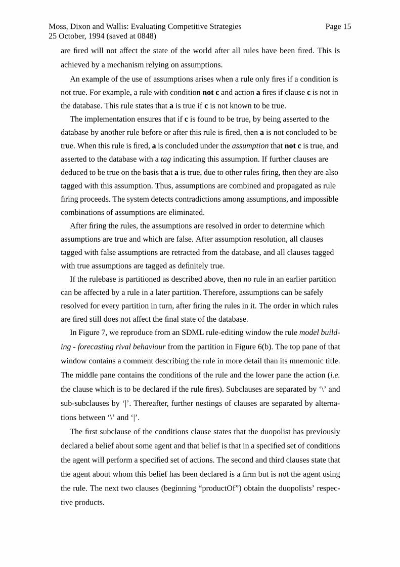
In Figure 7, we reproduce from an SDML rule-editing window the rulemodel build-

ing - forecasting rival behaviour from the partition in Figure 6(b). The top pane of that

window contains a comment describing the rule in more detail than its mnemonic title.

The middle pane contains the conditions of the rule and the lower pane the action (i.e.

the clause which is to be declared if the rule fires). Subclauses are separated by ‘\’ and

sub-subclauses by ‘|’. Thereafter, further nestings of clauses are separated by alterna-

tions between ‘\’ and ‘|’.

The first subclause of the conditions clause states that the duopolist has previously

declared a belief about some agent and that belief is that in a specified set of conditions

the agent will perform a specified set of actions. The second and third clauses state that

the agent about whom this belief has been declared is a firm but is not the agent using

the rule. The next two clauses (beginning “productOf”) obtain the duopolists’ respec-

tive products.


The subclause “clauseList ?believedConds and ?believedCondsList” is a special

kind of clause. The first word in every clause is a keyword. SDML keeps track of all

possible keywords and the syntax associated with each. Some can be asserted only to

public databases, some only to object-level databases and some only to meta-level

databases. All clauses with theclauseList keyword take three arguments: a clause, a

symbol and a list. The list, the clause or the symbol or some combination thereof must

be instantiated. If the list and the symbol are instantiated, then SDML instantiates the

pattern variable in the place of the clause with a clause starting with the symbol as key-

word and each element in the list as a subclause. If the clause is instantiated, then

SDML instantiates the symbol with the keyword of the clause and the list with a list of

the subclauses.

The reason for this is that lists are not logical clauses but they are easier to modify.

This is seen from the next few subclauses. Having constructed ?believedCondsList

from the clauses to which ?believedConds has been instantiated, the rule then checks

to see if that list includes the lagged clause “valueOf ?var ?ownProduct ?own-

VarValue” and, if it does, removes that clause from the list of clauses in

?believedCondsList.

There then follows a disjunctive clause looking in much the same way at the

believed actions. The disjuncts allow for the actions to be represented by a conjunctive

clause or by a single clause without subclauses. Either way, the issue is whether the

rival firm declares the current value of his decision variable as a response to some

lagged value of the agent using this rule.

The next four clauses in the conditions of this rule determine that the agent has

already specified a model in which the variable in question is determined in the market

directly by the value of the corresponding decision variable. In the Cournot model, for

example, supply determines sales exactly. In other models, the relationship is more

complex and requires the specification of a more elaborate relation between decision

variable and market variable.

As specified here, a model is always a list of clauses which have variables to be

determined by the model (the dependent clauses list), a list of instantiated clauses (the

dependent clauses list) which are in effect the arguments of the relation, and the

clauses which, given the variables instantiated in the independent clauses list, is able to

instantiate the variables of the dependent clauses list (the defining clauses list).

Figure 7near here


Of the remaining three clauses, the first two specify the elements of a new model.

The new defining clauses list is the existing list to which is appended a further clause

indicating that the value of the agent’s decision variable set this period will determine

the value of his rival’s decision variable (as reflected in its market counterpart) after

the lag indicated by the agent’s belief.

Finally, in the lower pane of the window is the clause to be asserted. All of the vari-

ables will have been instantiated by the conditions.

8 Conclusion

In this paper, we have run a round-robin tournament among matched pairs of smart

and dumb strategies. The dumb strategies were textbook, linear, Cournot reaction

functions and the smart strategies modified the dumb strategies in the light of experi-

ence and on the basis of models specified and developed by the smart agents. All of the

programming was done in SDML which ensures that the model of the environment

and the agents are represented as logical statements and inferences and that all infer-

ences are consistent. Moreover, to avoid nonsense results, the rules used to generate

these inferences have been written to avoid redundancy and conflicting outcomes such

as multiple levels of outputs. We thus achieve uniqueness as well as consistency. The

importance of the uniqueness and consistency of the inferences is that the experiments

reported here have a logical basis which has some identifiable degree of rigour. It

opens up the possibility of examining in other, more realistic models, the trade-off

between rigour and relevance.

Our results indicate that the representation of learning and expectations-formation

as a modelling procedure yields strategies which are robustly superior to (at least)

strategies represented by linear reaction functions. Obviously, there is much more to be

done here. Apart from using finer grids and, so, larger populations of strategies, it will

clearly be instructive to use more sophisticated dumb strategies involving random

selection of reaction functions, conjectural variations and multiple decision variables.

Nonetheless, we do claim to have demonstrated that scientifically constructed popu-

lations of strategies can be assessed for relative strength using a technique which gives

greatest weight to success in the most testing situations. The same testing procedure

can be applied to different approaches to strategy formation such as the smart and

dumb approaches identified here. Moreover, rigour can be maintained to the extent that

it is thought to be important in the specification and evaluation of these strategies.


References

Axelrod, R., (1990 ),The evolution of co-operation, (Penguin, London).

Chandler, A.D.Jr.(1962) Strategy and structure (Cambridge, Mass. and London:MIT

Press)

Chandler, A.D.Jr.(1977)The visible hand (Cambridge, Mass. : Harvard University

Press)

Cyert R.M.& March J.G (1963), A behavioral theory of the firm (Englewood Cliffs,

N.J.:Prentice Hall)

Dixon, H.D.,(1992) An algorithm for computing equilibrium supply and reaction

funtions, mimeo, University of York

Hart, O.D., (1985)Imperfect competition in general equilibrium: an overview,in: K.

Arrow and S. Honkapolja, eds., Frontiers of Economics (Basil Blackwell, Oxford).

Marshall, A.(1919), Industry and Trade (London: MacMillan).

Meyer, M. and P. Klemperer, (1989)Supply function equilibria under uncertainty, Econo-

metrica, 57, 1243-1271.

Moss, Scott, (1990)Control metaphors in the modelling of decision-making behaviour

University of Manchester Discussion Papers in Economics, 64

Penrose E. (1959), The theory of the growth of the firm (Oxford: Basil Blackwell)

Stanford, W.G., (1986) On continuous reaction function equilibria in duopoly supergames

with mean payoffs, Journal of Economic Theory, 39, 233-250.


Figure 1: Information flows in learning procedures

Agent’smodelling

procedures

Agent’sInternalModel

An Action

A Perception

Agent’sMemory of

Events

TheEnvironment

recording

reco

rdin

g

curr

ent

mod

el effects

effects

deco

ding

proc

ess

Ret

rievi

ng in

form

atio

n


Figure 2: The reaction-function-generating algorithm

1

1

A

x

IP2

x1

x2

R1

o

Ave

rag

e ri

val p

rofi

ts

Figure 3: Tournament results — average profits


Profit

Figure 4: Profit series in game between Firm-5 and Firm-3

Figure 5: Profit series in game between Firm-5 and Smart-Firm-3

Profit


Figure 6(a): Metarulebase dependency network: the start

Figure 6(b): Metarulebase dependency network: the finish


Figure 7: Metarule entitled model building - forecasting rival behaviou


.

Firm Intercept Slope

Firm-1 0.08 1.55556

Firm-2 0.44 0.555555

Firm-3 0.8 -0.444445

Firm-4 0.8 -0.722222

Firm-5 0.44 -0.222222

Firm-6 0.08 0.277778

Firm-7 0.44 -0.481482

Firm-8 0.8 -0.814815

Firm-9 0.8 -0.861111

Table 1: Generated reaction function parameters


Avg OwnProfit

Avg RivalProfit

Firm-5 0.090 0.073

Smart-Firm-1 0.089 0.094

Smart-Firm-9 0.089 0.105

Smart-Firm-2 0.087 0.062

Smart-Firm-4 0.082 0.066

Smart-Firm-3 0.082 0.051

Firm-7 0.082 0.120

Firm-1 0.075 0.043

Smart-Firm-7 0.075 0.117

Smart-Firm-8 0.074 0.089

Smart-Firm-5 0.072 0.073

Firm-2 0.068 0.027

Firm-6 0.064 0.115

Firm-8 0.063 0.045

Firm-4 0.060 0.030

Firm-9 0.059 0.059

Firm-3 0.057 0.017

Smart-Firm-6 0.052 0.137

Table 2: Average own and rivals’ profits in tournament


e = 0.01 0.1 3 5 50

18 SF-2 (0.308) SF-2 (0.316) SF-2 (0.481) SF-3 (0.54) SF-3 (0.68)

17 SF-3 (0.278) SF-3 (0.285) SF-3 (0.473) SF-2 (0.46) SF-2 (0.32)

16 SF-4 (0.204) SF-4 (0.200) SF-4 (0.045) SF-1 SF-1

15 SF-1 (0.204) SF-1 (0.199) SF-1 SF-4 SF-4

14 F-7 (0.005) F-5 F-5 F-5 F-5

13 F-5 F-7 SF-9 SF-9 SF-9

12 SF-9 SF-9 F-1 F-1 F-1

11 SF-8 SF-8 F-7 F-7 F-7

10 SF-7 SF-7 SF-7 SF-7 SF-7

9 F-1 F-1 SF-8 SF-8 SF-8

8 SF-5 SF-5 F-9 F-9 F-9

7 F-6 F-6 SF-5 SF-5 SF-5

6 F-2 F-2 SF-6 SF-6 SF-6

5 F-8 F-8 F-6 F-6 F-6

4 F-4 F-9 F-2 F-2 F-2

3 F-9 F-4 F-8 F-8 F-8

2 SF-6 SF-6 F-3 F-3 F-3

1 F-3 F-3 F-4 F-4 F-4

Table 3: Order of extinction or survival strength (% surviving population )SF-n = Smart-Firm-n; F-n = Firm-n

Documents

Evaluating Competitive Strategies - Huw Dixonhuwdixon.org/publication_archive/articles/evaluating...Moss, Dixon and Wallis: Evaluating Competitive Strategies Page 3 25 October, 1994