evaluating atmospheric methane inversion model results for

Boreal environment research 20: 506–525 © 2015issn 1239-6095 (print) issn 1797-2469 (online) helsinki 28 august 2015

Editor in charge of this article: Veli-Matti Kerminen

evaluating atmospheric methane inversion model results for Pallas, northern Finland

aki tsuruta1)*, tuula aalto1), leif Backman1), Wouter Peters2), maarten Krol2), ingrid t. van der laan-luijkx2), Juha hatakka3), Pauli heikkinen4), edward J. Dlugokencky5), renato spahni6) and nina n. Paramonova7)

1) Finnish Meteorological Institute, Climate Research, P.O. Box 503, FI-00101 Helsinki, Finland (*corresponding author’s e-mail: [email protected])

2) Wageningen University, Meteorology and Air Quality, P.O. Box 47, NL-6700AA Wageningen, the Netherlands

3) Finnish Meteorologiacal Institute, Atmospheric Composition Research, P.O. Box 503, FI-00101 Helsinki, Finland

4) Finnish Meteorological Institute, Arctic Research, Tähteläntie 62, FI-99600 Sodankylä, Finland5) NOAA Earth System Research Laboratory, Boulder, Colorado 80305, USA6) University of Bern, Climate and Environmental Physics, Physics Institute, Oeschger Centre for

Climate Change Research, Sidlerstrasse 5, CH-3012 Bern, Switzerland7) Voeikov Main Geophysical Observatory, Karbyshev str. 7, RU-194021 St. Petersburg, Russia

Received 9 June 2014, final version received 3 Jan. 2015, accepted 19 Nov. 2014

tsuruta a., aalto t., Backman l., Peters W., Krol m., van der laan-luijkx i.t., hatakka J., heikkinen P., Dlugokencky e.J., spahni r. & Paramonova n.n. 2015: evaluating atmospheric methane inversion model results for Pallas, northern Finland. Boreal Env. Res. 20: 506–525.

A state-of-the-art inverse model, CarbonTracker Data Assimilation Shell (CTDAS), was used to optimize estimates of methane (CH4) surface fluxes using atmospheric observations of CH4 as a constraint. The model consists of the latest version of the TM5 atmospheric chemistry-transport model and an ensemble Kalman filter based data assimilation system. The model was constrained by atmospheric methane surface concentrations, obtained from the World Data Centre for Greenhouse Gases (WDCGG). Prior methane emissions were specified for five sources: biosphere, anthropogenic, fire, termites and ocean, of which bio-sphere and anthropogenic emissions were optimized. Atmospheric CH4 mole fractions for 2007 from northern Finland calculated from prior and optimized emissions were compared with observations. It was found that the root mean squared errors of the posterior esti-mates were more than halved. Furthermore, inclusion of NOAA observations of CH4 from weekly discrete air samples collected at Pallas improved agreement between posterior CH4 mole fraction estimates and continuous observations, and resulted in reducing optimized biosphere emissions and their uncertainties in northern Finland.

Introduction

Methane (CH4) is one of the most effective greenhouse gases. It’s global warming potential over a 100 year time horizon is 28 times that of

carbon dioxide (IPCC 2013: chapter 8.7), and its atmospheric burden more than doubled since 1750 (MacFarling Meure et al. 2006, Rhodes et al. 2013). Anthropogenic emissions are the main reason for the increase up to the1980s

Boreal env. res. vol. 20 • Evaluation of atmosheric methane inversion model 507

(Rasmussen and Khalil 1981, Khalil and Ras-mussen 1985). In the 1990s, the annual growth rate decreased, and became nearly zero in the early 2000s. Several reasons have been proposed to explain the variations: a decline in the emis-sions from biogenic sources, such as wetlands and rice, in the northern hemisphere (Kai et al. 2011), a decline in the fossil fuel emissions (Aydin et al. 2011), or an increase in the main sink of CH4 reaction with atmospheric OH (Krol et al. 1998, Bousquet et al. 2006, Monteil et al. 2011). However, if lifetime and emission were constant, decrease in growth rate is an indica-tor that atmosphere is reaching a steady state (Dlugokencky et al., 2011). Furthermore, the concentration started to increase again in 2006 (Rigby et al. 2008), and the exact reasons are still unknown (Dlugokencky et al. 2009, Hei-mann 2011).

Several inverse modeling studies assessed the reasons for the changes in the methane growth rate (Bergamaschi et al. 2005, 2007, 2010, 2013, Bousquet et al. 2005, 2011, Bruhwiler et al. 2014, Houweling et al. 2014). Inverse model-ing, which optimizes emissions from different source categories, is a powerful tool for under-standing changes in the emissions from both human activities and nature. The main sources of anthropogenic emissions are agriculture, waste and fossil fuels, whereas biosphere emissions are dominated by wetlands (Kirschke et al. 2013). Anthropogenic emissions are responsible for long-term and inter-annual variability of atmo-spheric methane, whereas biosphere emissions have large effects on seasonal cycles. Global methane emission is estimated to be around 500–600 Tg y–1, and for Europe 35–60 Tg y–1, where anthropogenic emissions also dominate (Kirschke et al. 2013 and references therein). However, the estimates vary substantially among models and model settings. Although the vari-ation among inverse modeling estimates are smaller than for process models, the choice of transport model (Locatelli et al. 2013), obser-vation data sets (Alexe et al. 2014, Villani et al. 2010) and prior emission distributions affect the results.

In this study, we evaluated the performance of a state-of-the-art inverse model system based on the data assimilation system CTDAS

(Carbon Tracker Data Assimilation Shell, see http://www.carbontracker.eu/ctdas/) for boreal sites of northern Finland in 2007. The system contains the latest version of the atmospheric chemistry-transport model TM5 (Krol et al. 2005) driven by the European Centre for Medium-Range Weather Forecasts (ECMWF) ERA-Interim meteorological fields. TM5 is used with a two-way nested European domain with a 1° ¥ 1° grid over Europe and high northern lati-tudes. Here, observations of atmospheric CH4 for 2007 from NOAA’s global cooperative air sam-pling network and other discrete air sampling networks were used to constrain the emissions in the model. The discrete air sample data have been used extensively as constraints in surface flux inversion studies based on data assimilation (Bergamaschi et al. 2007, Bruhwiler et al. 2014, Houweling et al. 1999).

To examine the performance of the inverse model for boreal areas, especially northern Fin-land, the modeled atmospheric concentrations estimated using the emissions before and after optimization of the emissions were compared with model-independent continuous observa-tions for 2007. Furthermore, two inversions, one with and one without assimilating the Pallas discrete air sample observations were compared to test the effects of the Pallas observations in the inverse model results.

Methods and data sets

CTDAS atmospheric inverse model

CTDAS is a pyshell version of CarbonTracker, developed by NOAA-ESRL (National Oceanic and Atmospheric Administration’s Earth System Research Laboratory) and the Wageningen Uni-versity. The model had originally been designed to optimize carbon dioxide fluxes (Peters et al. 2005), and it has been further developed for CH4 by Bruhwiler et al. (2014) and in this study (European CarbonTracker-CH4). Models devel-oped by Bruhwiler et al. (2014) and in this study differ to certain extent: the emission sources that are optimized, the geographical area of focus, i.e. the zoom grid in the TM5 transport model, prior emissions such as anthropogenic and biosphere,

508 Tsuruta et al. • Boreal env. res. vol. 20

observations assimilated, and source region boundaries are different from their studies.

The optimal weekly mean CH4 fluxes F(r,t) in region r and time t (week) were calculated as follows:

F(r,t) = λbio(r,t)Fbio(r,t) + λanth(r,t)Fanth(r,t) + Ffire(r,t) + Fterm(r,t) + Foce(r,t), (1)

where Fbio, Fanth, Ffire, Fterm, Foce are the emissions

from biosphere, anthropogenic activities, fire, termites and ocean, respectively. The scaling fac-tors for the biosphere and anthropogenic emis-sions are optimized in the model.

In order to assess the influence of the NOAA Pallas flask measurements on the optimized fluxes for European and boreal regions, we per-formed two runs: S1 including all the measure-ments listed in Table 1, and S2 excluding the Pallas flask measurements.

Table 1. list of sites used in european carbontracker-ch4. the model data mismatch (mdm) was used as the observation error. observations were rejected in the assimilation if the estimated mole fractions were not within 3 ¥ observation error. note that only observations from discrete air samples were used.

site station name country/ contributor lat. long. elevation mdmcode territory (°n) (°e) (m a.s.l.) (ppb)

abp arembepe Brazil noaa/esrl –12.77 –38.17 0.0 7.5alt alert canada noaa/esrl 82.72 –62.52 210.0 15.0ams amsterdam island France noaa/esrl –37.8 77.53 55.0 7.5amt argyle Usa noaa/esrl 45.03 –68.68 50.0 30.0arh arrival heights new Zealand niWa –77.8 166.67 184.0 7.5asc ascension island UK noaa/esrl 7.55 14.25 54.0 7.5ask assekrem algeria noaa/esrl 23.27 5.63 2710.0 25.0azr terceira island Portugal noaa/esrl 38.77 –27.37 40.0 15.0bal Baltic sea Poland noaa/esrl 55.35 17.22 28.0 75.0bgu Begur spain lsce 41.97 3.23 13.0 15.0bhd Baring head newZealand noaa/esrl –41.41 174.87 85.0 7.5bkt Bukit Koto tabang indonesia noaa/esrl –0.2 100.32 864.5 75.0bme st. David’s head UK noaa/esrl 32.37 –64.65 30.0 15.0bmw tudor hill UK noaa/esrl 32.27 –64.87 30.0 15.0brw Barrow Usa noaa/esrl 71.32 –156.6 11.0 15.0bsc Black sea romania noaa/esrl 44.17 28.67 3.0 75.0cba cold Bay Usa noaa/esrl 55.20 –162.72 25.0 15.0cfa cape Ferguson australia csiro –19.28 147.05 2.0 25.0cgo cape Grim australia noaa/esrl –40.68 144.68 94.0 7.5chr christmas island Kiribati noaa/esrl 1.70 –157.17 3.0 7.5crz crozet France noaa/esrl –46.45 51.85 120.0 7.5cya casey station australia csiro –66.28 110.53 60.0 7.5eic easter island chile noaa/esrl –27.13 –109.45 50.0 7.5esp estevan Point canada ec 49.38 –126.55 39.0 25.0esp estevan Point canada csiro 49.38 –126.55 39.0 25.0fik Finokalia Greece LSCE 35.34 25.67 150.0 15.0gmi Guam Usa noaa/esrl 13.43 144.78 2.0 15.0hba halley Bay UK noaa/esrl –75.57 –26.5 33.0 7.5hpb hohenpeissenberg Germany noaa/esrl –75.57 11.02 985.0 25.0hun hegyhatsal hungary noaa/esrl 46.95 16.65 248.0 75.0ice heimaey iceland noaa/esrl 63.40 –20.28 100.0 15.0izo izaña spain noaa/esrl 28.30 –16.5 2367.0 15.0key Key Biscayne Usa noaa/esrl 25.67 –80.2 3.0 25.0kum cape Kumukahi Usa noaa/esrl 19.52 –154.82 3.0 7.5kzd sary taukum Kazakhstan noaa/esrl 44.45 75.57 412.0 75.0kzm Plateau assy Kazakhstan noaa/esrl 43.25 77.87 2519.0 25.0lln lulin china noaa/esrl 23.47 120.87 2867.0 25.0lmp lampedusa italy noaa/esrl 35.52 12.63 45.0 25.0

continued


Table 1. continued.

site station name country/ contributor lat. long. elevation mdmcode territory (°n) (°e) (m a.s.l.) (ppb)

lpo ile Grande France lsce 48.80 –3.58 10.0 15.0maa mawson australia csiro –67.62 62.87 32.0 7.5mhd mace head ireland noaa/esrl 53.33 –9.9 8.0 25.0mid sand island Usa noaa/esrl 28.20 –177.37 7.7 15.0mlo mauna loa Usa noaa/esrl 19.54 –155.58 3397.0 15.0mqa macquarie island australia csiro –54.48 158.97 12.0 7.5nmb Gobabeb namibia noaa/esrl –23.57 15.02 461.0 25.0nwr niwot ridge Usa noaa/esrl 40.05 –105.59 3523.0 15.0oxk ochsenkopf Germany noaa/esrl 50.03 11.80 1185.0 75.0pal Pallas-sammaltunturi Finland noaa/esrl 67.97 24.12 560.0 15.0pdm Pic du midi France lsce 42.94 0.14 2877.0 15.0psa Palmer station Usa noaa/esrl –64.92 –64 10.0 7.5pta Point arena Usa noaa/esrl 38.95 –123.72 17.0 25.0puy Puyde Dome France lsce 45.77 2.97 1465.0 15.0rpb ragged Point Barbados aGaGe 13.17 –59.43 45.0 15.0sey mahe island seychelles noaa/esrl –4.67 55.17 7.0 7.5sgp southern Great Plains Usa noaa/esrl 36.78 –97.5 314.0 75.0shm shemya island Usa noaa/esrl 52.72 174.08 40.0 25.0smo tutuila Usa aGaGe –14.24 –170.57 42.0 7.5spo south Pole Usa noaa/esrl –89.98 –24.8 2810.0 7.5stm ocean station m norway noaa/esrl 66.00 2.00 5.0 15.0sum summit Denmark noaa/esrl 72.58 –38.48 3238.0 15.0syo syowa station Japan noaa/esrl –69 39.58 16.0 7.5tap tae-ahn Peninsula Korea noaa/esrl 36.72 126.12 20.0 75.0tdf tierradel Fuego argentina noaa/esrl –54.87 –68.48 20.0 7.5ter teriberka russia mGo 69.20 35.10 40.0 15.0thd trinidad head Usa noaa/esrl 41.05 –124.15 120.0 7.5uta Wendover Usa noaa/esrl 39.88 –113.72 1320.0 25.0uum Ulaan Uul mongolia noaa/esrl 44.45 111.08 914.0 25.0wis sede Boker israel noaa/esrl 31.12 34.87 400.0 25.0wkt moody Usa noaa/esrl 31.32 –97.32 708.0 30.0wlg mt. Waliguan china noaa/esrl 36.28 100.90 3810.0 15.0wsa sable island canada ec 43.93 –60.02 5.0 25.0zep Zeppelinfjellet norway noaa/esrl 78.90 11.88 475.0 15.0

TM5 atmospheric transport model

The link between atmospheric CH4 measure-ments and exchange of CH4 at the Earth’s sur-face is the transport of CH4 in the atmosphere. In our assimilation system, the release 3 of the TM5 chemistry transport model was used as the lin-earized observation operator. TM5 was run with a 1° ¥ 1° zoom region over Europe (24–74°N, 21°W–45°E), framed by an intermediate grid of 2° ¥ 3° for outer Europe, and 4° ¥ 6° glob-ally (Fig. 1), driven by ECMWF ERA-Interim meteorological fields. Atmospheric chemical loss was calculated using off-line chemistry with monthly tropospheric OH concentrations (Hou-

weling et al. 2014). Furthermore, stratospheric sink due to reaction with OH, Cl and O(1D) were included by applying reaction rates based on a 2D photochemical Max-Planck-Institute (MPI) model (Bergamaschi et al. 2005). The global total atmospheric chemical loss, i.e. the integrat-ing OH, Cl and O(1D) losses during 2007, was about 511 Tg CH4 y–1, with a methane lifetime of about 9.6 years defined by the global burden divided by the loss.

In this work, atmospheric mole fractions were estimated using the TM5 forward model. The mole fractions estimated with prior emis-sions are henceforth called ‘prior’, and the esti-mates with posterior emissions ‘posterior’.


Prior CH4 flux data sets

The prior data sets consisted of anthropogenic, biosphere, fire, termite and ocean emissions, col-lected from inventories and studies outside this project. Total posterior emissions were calcu-lated using Eq. 1. All emission fields were grid-ded to match the finest TM5 grid, i.e., 1° ¥ 1°, globally.

Anthropogenic methane emissions are responsible for more than half of the global meth-ane source. For monthly mean anthropogenic emissions, the Emission Database for Global Atmospheric Research ver. 4.2 (EDGARv4.2) was used. The emissions from agricultural waste burning and large scale biomass-burning were removed, because they overlap with fire emis-sions described later. The annual anthropogenic emission for 2007 was 337 Tg CH4 y

–1 (exclud-ing fires), in which agricultural emissions, such as enteric fermentation (99 Tg CH4 y–1) and agricultural soils (36 Tg CH4 y–1), and fugitive emissions from oil and gas (66 Tg CH4 y

–1) and solid fuels (43 Tg CH4 y–1) dominated. We did not introduce seasonal variations in the anthro-pogenic emissions.

Natural emissions, dominated by wetlands, are estimated to contribute about 40% of the total emissions, where inter-annual variability of emissions from wetland ecosystems is esti-mated to be ±12 Tg CH4 y

–1 (Spahni et al. 2011). For monthly-mean biosphere emissions, the esti-mates by the LPJ-WHyMe vegetation model (Spahni et al. 2011) were used. The emissions from rice fields were removed since they were already included in the anthropogenic emissions. EDGARv4.2 estimates of the emissions from rice fields were ca. 6 Tg CH4 y–1 smaller than LPJ-WHyMe estimates; no scaling was applied to the EDGARv4.2 estimates. The annual bio-sphere emission for 2007 was 160 Tg CH4 y–1 (excluding rice fields), with the seasonal cycle already captured in the prior.

Methane emissions from natural fires account for less than 10% of the global total (Kirschke et al. 2013). These emissions are an important part of the carbon cycle and their inter-annual variability can be large because of occasional intense fires and events, such as strong El Niño that lead to dry periods around the equator (Lan-genfelds et al. 2002). Also, the spatial variability of fire emissions should be taken into account

30W 0 30E 60EEQ

30N

60N

90N

Fig. 1. tm5 zoom grid definition used in the european carbontracker-ch4.


(Andreae and Merlet 2001). Monthly-mean fire emissions from the Global Fire Emissions Data-base ver. 3.1 (GFEDv3.1) were used. The data set contained both natural and anthropogenic fire emissions (van der Werf et al. 2010), includ-ing agricultural waste burning and large-scale biomass burning with seasonal cycles captured. Annual total fire emissions for 2007 were 17.44 Tg CH4 y

–1 in GFEDv3.1, and 30.36 Tg CH4 y–1

in EDGARv4.2.Methane emissions of termites accounts for

about 5% of global emissions, but the spatial variability of these emission should be taken into account. Annual-mean termite emissions from Ito et al. (2012) were used. The emissions were estimated based on Fung et al.’s (1991) up-scal-ing method, biome-specific termite biomass den-sity and emission factors were obtained from Fraser et al. (1986), and a historical land cover map based on Hurtt et al. (2006) was used to introduce inter-annual variability. The average termite biomass density in boreal forests was assumed to be zero. We did not introduce sea-sonal variations into the termites emissions. In this study, emissions for 2007 were assumed to be the same as the latest estimate, i.e. of 2006.

Methane emissions from open oceans are a relatively minor, about 0.2% of the global emis-sions. Monthly-mean ocean emission fields were pre-calculated based on seasonal meth-ane saturation ratios from Bates et al. (1996), which were derived from measurements of sea-water and atmospheric methane mixing ratios throughout the Pacific Ocean. The saturation ratios were used globally as zonal averages. The difference between air and seawater par-tial pressures of methane, dp(CH4), was calcu-lated using saturation ratios. The zonal monthly mean dry air CH4 mixing ratios were taken from GLOBALVIEW-CH4 (Cooperative Atmospheric Data Integration Project — Methane, see www.esrl.noaa.gov/gmd/ccgg/globalview/ch4/ch4_intro.html). Sea level pressure, sea surface tem-perature, sea-ice concentration and 10 meter wind speeds were from the ECMWF ERA-interim data (Dee at al. 2011). Solubility of methane in seawa-ter was calculated according to Wiesenburg and Guinasso (1979), assuming salinity of 35‰. Gas transfer velocity was parametrized using the wind speed and Schmidt number (Wanninkhof 1992).

Fluxes were then calculated as the product of gas transfer velocity, gas solubility and dp(CH4). Sea-ice was assumed to inhibit gas transfer.

Atmospheric methane observations

Global methane atmospheric measurements were obtained from the World Data Centre for Green-house Gases (WDCGG). Measurements are from the NOAA, CSIRO, EC, LSCE, NIWA and MGO discrete air samples, and background measure-ments were selected according to each contribu-tor’s quality control flags. The location of each site is shown in Fig. 2. The model data mismatch (mdm), used for the criteria of observation rejec-tion thresholds and observation error covariance matrix, was defined by site types: 7.5 ppb for marine boundary layer and high southern hemi-sphere sites, 15 ppb for mixed sites, 25 ppb for land and tower sites, 30 ppb for sites with large variability in observations, and 75 ppb for so called “problematic” sites. For the list and details of the measurement sites, see Table 1. The obser-vations were rejected in the assimilation if esti-mated concentrations were not within three times the measurement errors. The number of meas-urements available varied by site, but around 70 measurements were assimilated per week.

To assess the model results in the European boreal regions, two independent observation data sets from northern Finland were compared with the TM5-estimated CH4 mole fractions using the prior and posterior emissions. The data sets were the FMI continuous atmospheric measurements from Pallas (Aalto et al. 2007), and the Fourier transform infrared spectroscopy (FTIR) mea-surements from Sodankylä (Kivi et al. 2014).

Pallas is located at 67.58°N and 24.06°E (565 m a.s.l.), where its main station Sammal-tunturi is located on the top of a hill. About 6% of the nearest 20 km2 consists of open wetland, and the area is sparsely populated. During 2007, CH4 was measured four times per hour with an automated gas chromatographic system (Agilent 6890N) equipped with a flame ionization detec-tor for CH4 detection. The measurements are cal-ibrated using standards on the WMO/CCL scale (Aalto et al. 2007). Hourly mean observations for day and night were used.


Sodankylä is located at 67.36°N, 26.63°E (179 m above mean sea level), about 150 km southeast of Pallas, and a FTIR instrument has been operated at the site since February 2009. The FTIR instrument in Sodankylä acquires solar spectra using a Bruker 125HR Fourier transform spectrometer. The instrument is participating in the Total Carbon Column Observing Network (TCCON, http://www.tccon.caltech.edu/), and the total column measurements were processed using the standard approach used in the network (Wunch et al. 2011). Due to its high-latitude location, there is little or no sunlight during winter, FTIR observations between November and January are discuntinued. Monthly means and standard deviations of the measurements were calculated using all data from 2009–2012. Note that the inverse model was run for 2007, so we compare only the shapes of the seasonal cycle with the model estimates. Note that Sodan-kylä is both spatially and temporally a mod-el-independent site; i.e., no measurements from Sodankylä were used in this study.

TransCom and land-ecosystem regions

We optimized fluxes region-wise, where the

regions r in Eq. 1 were defined by TransCom and land-ecosystem maps. The global surface was divided into 16 regions, based on the TransCom regions used in Peters et al. (2007), except that oceans were aggregated into one region and Europe was divided into four subregions (Fig. 3). Further, terrestrial areas were divided based on soil types, because methane emissions are affected by soil properties (Matthews and Fung 1987, Yvon-Durocher et al. 2014). Land-ecosys-tem regions were defined mainly based on Pri-gent et al. (2007) and Wania et al. (2010), also used in LPJ-WHyMe vegetation model (Spahni et al. 2011). The regions consisted of six types of land ecosystems (Fig. 4): inundated wetland and peatland (IWP), wet mineral soil (WMS), rice (RIC), anthropogenic land (ANT), water (WTR) and ice (ICE). Each grid point was therefore defined by TransCom and land-eco-system region. The land-ecosystem map was not dynamic and did not change during the year. The prior scaling factors were all equal to one: λ = (λbio, λanth) = (1, 1, ..., 1) = 1. For land-ecosystem region IWP and WMS, biosphere emissions were optimized, i.e. λanth = 1, and for RIC, ANT and WTR, anthropogenic emissions were optimized, i.e. λbio = 1. Theoretically, this approach results in 72 (14 TransCom ¥ 5 land-ecosystem + ocean

180°W 90°W 0 90°E 180°E90°S

60°S

30°S

EQ

30°N

60°N

90°N

abp

alt

ams

amt

arh

asc

ask

azr

bal

bgu

bhd

bkt

bmebmw

brw

bsccba

cfa

cgo

chr

crz

cya

eic

espesp

fik

gmi

hbahpb

hun

ice

izokeykum

kzdkzm

llnlmp

lpo

maa

mhd

mid

mlo

mqa

nmb

nwr

oxk

pal

pdm

psa

pta

puy

rpbsey

sgp

shm

smo

spo

stmsum

syo

tap

tdf

ter

thd uta uum

wiswkt wlgwsa

zep

Fig. 2. locations (black dots) of the sites from which the data were assimilated in european carbontracker- ch4 for 2007. For site-name codes see table 1.


180W 120W 60W 0 60E 120E 180E90S

60S

30S

EQ

30N

60N

90N

(1)North American boreal

(2)North American temperate

(3)South American tropical

(4)South American temperate

(5)Northern Africa

(6)Southern Africa

(7)Eurasian boreal

(8)Eurasian temperate

(9)Tropical Asia

(10)Australia

(11) SouthwesternEurope

(12) Southeastern Europe

(13) NorthwesternEurope

(14) NortheasternEurope

(15) Ocean

(16) Ice

(16) Ice

Fig. 3. the land regions in european carbon-tracker-ch4. they are defined according to the transcom regions, except for europe, which is divided into four sub-regions.

180W 120W 60W 0 60E 120E 180E90S

60S

30S

EQ

30N

60N

90N

(1)Inundated wetland,

peatland

(2)Wet mineral soil

(3)Rice

(4)Anthropogenic

(5)Water

(6)Ice

Fig. 4. land-ecosystem map used for european carbontracker-ch4.

+ ice) state-vector elements each week. How-ever, some TransCom regions contain fewer than five ecosystems types, and for ICE, emissions were assumed to equal zero for both prior and posterior. Therefore, the actual number of scal-ing factors λ = (λbio, λanth) to be optimized was 49 per week globally.

Results

Comparison with Pallas continuous observations

The mismatch between simulated CH4 and observations indicates that using the prior fluxes generally results in overestimations of CH4


abundance at Pallas (Fig. 5). The prior matches the observations fairly well in the beginning of the year, but the baseline increases faster than in the observations, reaching ca. 20 ppb higher values at the end of the year. Peaks in the prior during summer and autumn were much higher than in the observations, pointing to prior CH4 fluxes that are too large.

As expected, the hourly S1 posterior con-centrations matched the FMI hourly continuous observations better than the prior concentrations (Fig. 5). The unrealistically strong seasonal cycle in the prior was improved in the posterior. As a result of the lower posterior wetland emis-sions, the peaks in the posterior concentrations were much lower that those in the prior, espe-cially during summer and autumn, matching the observed concentrations better throughout the year. The large increase in the baseline of the prior concentrations in summer and autumn

was attributed to an overestimation in biosphere emissions. Wetland fractions for the region may be overestimated in the prior emission calcula-tion (Prigent et al. 2007). There was a consider-able mismatch between posterior concentrations and the observations around the end of Sep-tember, when the posterior concentrations were much higher than the observed ones. Although better than the prior, maximum differences in the posterior concentrations were still up to 200 ppb. Note that there was often only one obser-vation per site per week assimilated during the inversion, and during some weeks, observations from Pallas and nearby sites such as Terib-erka and Zeppelinfjellet, were rejected from the assimilation (Fig. 6). The number of rejected observations was greatest in autumn, includ-ing the period when the maximum differences were estimated. For the rejected observations, the modeled concentrations were 45.0 ppb, or

1850

1950

2050

2150

CH

4 (p

pb)

Observationprior

1850

1950

2050

2150Observationposterior S1

1850

1950

2050

2150Observationposterior S2

Jan Feb Mar Apr May Jun Jul Aug Sep Oct Nov Dec–100

–50

0

50

100S1 – S2

Fig. 5. measured and modeled atmospheric methane for 2007 at Pallas. thick gray lines are Fmi continuous mea-surements, and thin back lines show modeled mole fractions using prior (top), weekly posterior with (s1) and with-out (s2) assimilating Pallas noaa measurements from discrete air samples. the bottom panel shows differences between the s1 and s2 posterior fractions.


more, greater than the observed concentrations, probably resulted from too high prior emis-sion estimates. The highest concentration in the observations (1947 ppb) at Teriberka in Novem-ber was unintentionally added to the assimilation data set. This observation should have been removed during the preprocessing because it was rejected, according to the flag assigned by the data provider, as not being representative of background conditions.

The S2 posterior concentrations also generally better match the observations than the prior. Com-pared with the S1 posterior, the baseline of the two were similar during winter and spring, but S2 baseline was lower than that of S1 in summer, and slightly higher in autumn (Fig. 5).

The annual mean of the residuals between the observations and prior concentrations again showed that the prior estimates were generally higher than the observations; a histogram of the residuals was positively skewed, and the root mean square error (RMSD) was about 1.5 times greater than the standard deviation (Fig. 7). The residuals using the S1 posterior mole fractions were closer to normal distribution (the left and right tails of the histogram are almost equally long), the mean of the residuals was much closer

to zero than that of the prior, and the differences between the standard deviation and the RMSD was only about 0.2 ppb. This confirms that the S1 posterior matched the observations better than the prior. Comparing the residuals of the S1 and S2 posterior, the mean residual was about 4 ppb greater in S2, the S2 standard deviation was a little greater, and RMSD was not as close to its standard deviation as that in S1. Thus, the S1 residuals at Pallas more closely resemble a normal distribution as compared with the S2 residuals, and the S1 mole fractions matched the observations better. Some outliers were seen in the S1 residuals, which mainly resulted from the high concentrations estimated in autumn.

Next, two test runs with TM5 were per-formed to assess the effect of the anthropogenic and biosphere emissions on the methane con-centration at Pallas. TM5 was run using the S1 posterior emissions with either the European anthropogenic emissions or the European bio-sphere emissions artificially set to zero (Fig. 8). Here, Europe was defined as an aggregate of four regions: northeast, northwest, southeast and southwest Europe. The posterior concen-trations (Fig. 8a) indicate that the baseline was lower than the observations throughout the year

1840

1860

1880

1900

1920

1940

1960a

b

CH

4 (p

pb)

Jan Feb Mar Apr May Jun Jul Aug Sep Oct Nov Dec–150

–100

–50

0

50

100

150

Res

idua

l (pp

b)

Pallas Zeppelinfjellet Teriberka

Fig. 6. (a) time series of noaa and mGo measurements: dots are assimilated measurements, and squares are rejected. (b) Differences between prior and measured for each measurements: gray lines are the rejection thresh-olds of –45 and 45 ppb for all three sites. measurements were rejected when the difference exceeded the rejection threshold.


–200 –100 0 100 200

100

300

500

700

900

1100

1300 a

mean = 60.04SD = 48.16RMSD = 76.97

–200 –100 0 100 200

b

mean = 2.66SD = 21.75RMSD = 21.92

–200 –100 0 100 200

c

mean = 6.05SD = 22.44RMSD = 23.24

1850

1950

2050

2150

CH

4 (p

pb)

a

Jan Feb Mar Apr May Jun Jul Aug Sep Oct Nov Dec

1850

1950

2050

2150

CH

4 (p

pb)

b

Fig. 7. histograms and statistics of the residuals between Fmi continuous observations and tm5-modeled mole fractions using (a) prior, and weekly posterior emissions optimized (b) with and (c) without noaa Pallas observa-tions assimilated for 2007. note the prior emissions were monthly. the root-mean-square deviation (rmsD) = [Σ(estimate – measurement)2/n]1/2. Units of the x-axis and the statistics are parts per billion (ppb).

Fig. 8. measured and modeled atmospheric methane for 2007 at Pallas. thick grey lines are Fmi continuous obser-vations, and thin red lines show modeled mole fractions using weekly posterior emissions, in which the european (a) anthropogenic and (b)biosphereemissionswereartificiallysettozero.

when European anthropogenic emissions were excluded. Without European anthropogenic emissions, simulated CH4 failed to capture most of the peaks during winter and spring, but the summer and autumn peaks were well captured. Some peaks in late autumn and small peaks during winter and spring were seen episodically at Pallas, which may be due to long-range trans-

port from Russia (Siberia). The posterior mole fractions (Fig. 8b) indicate that the baseline follows the observations well in the beginning of the year and throughout the spring, but it was too low during the rest of the year. Winter and spring peaks were well captured (see Fig. 8b), but only few of summer and autumn peaks were gener-ated. This shows that winter and spring concen-


trations at Pallas contain mainly anthropogenic signals, whereas summer and autumn concen-trations are affected by the biosphere emissions.

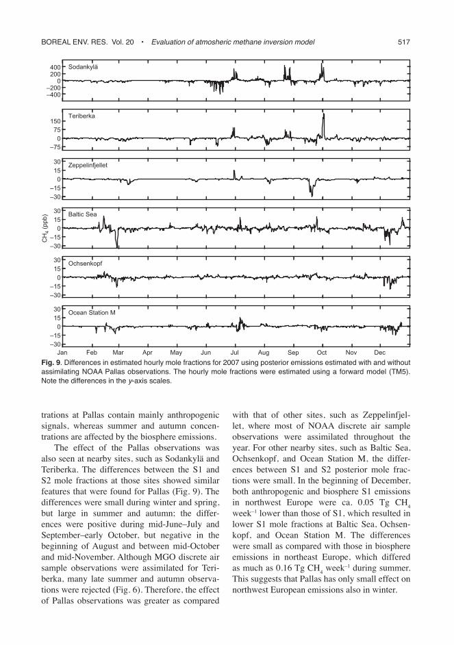
The effect of the Pallas observations was also seen at nearby sites, such as Sodankylä and Teriberka. The differences between the S1 and S2 mole fractions at those sites showed similar features that were found for Pallas (Fig. 9). The differences were small during winter and spring, but large in summer and autumn; the differ-ences were positive during mid-June–July and September–early October, but negative in the beginning of August and between mid-October and mid-November. Although MGO discrete air sample observations were assimilated for Teri-berka, many late summer and autumn observa-tions were rejected (Fig. 6). Therefore, the effect of Pallas observations was greater as compared

with that of other sites, such as Zeppelinfjel-let, where most of NOAA discrete air sample observations were assimilated throughout the year. For other nearby sites, such as Baltic Sea, Ochsenkopf, and Ocean Station M, the differ-ences between S1 and S2 posterior mole frac-tions were small. In the beginning of December, both anthropogenic and biosphere S1 emissions in northwest Europe were ca. 0.05 Tg CH4 week–1 lower than those of S1, which resulted in lower S1 mole fractions at Baltic Sea, Ochsen-kopf, and Ocean Station M. The differences were small as compared with those in biosphere emissions in northeast Europe, which differed as much as 0.16 Tg CH4 week–1 during summer. This suggests that Pallas has only small effect on northwest European emissions also in winter.

–400–200

0200400

CH

4 (p

pb)

Sodankylä

–750

75150

Teriberka

–30–15

01530 Zeppelinfjellet

–30–15

01530 Baltic Sea

–30–15

01530 Ochsenkopf

Jan Feb Mar Apr May Jun Jul Aug Sep Oct Nov Dec–30–15

01530 Ocean Station M

Fig. 9. Differences in estimated hourly mole fractions for 2007 using posterior emissions estimated with and without assimilating noaa Pallas observations. the hourly mole fractions were estimated using a forward model (tm5). note the differences in the y-axis scales.


The seasonal cycle in Sodankylä column averaged mixing ratio

Here, we compare Sodankylä FTIR observations with modeled column averaged mixing ratios of methane (XCH4). The Sodankylä XCH4 data were not assimilated in the model. Detrended monthly averages of the XCH4 observations were calculated using all data of the period 2009–2012, and the model data from 2007. Note that the observations and the model data do not overlap.

The monthly column-averaged mixing ratios for 2007 were estimated with TM5 using the prior and posterior emissions for the 1° ¥ 1° grid box containing Sodankylä. Monthly statis-tics were calculated from daily 3D atmospheric concentration fields, and the annual mean was subtracted to compare the shapes of the seasonal cycle with that of Sodankylä FTIR measure-ments (Fig. 10). The mean of all the measure-ments was subtracted to calculate the anomalies of the measurements. The observations showed a XCH4 decrease in spring, and an increase from the summer towards winter. The prior estimates failed to capture the shape of the seasonal cycle of the observations. The prior showed ca. 20 ppb XCH4 increase from the beginning to the end of the year, whereas the observations showed no such increase. The shape of posterior estimates matched the observations better; the means and

standard deviations of the anomalies were within the two standard deviations of the anomalies of the measurements throughout the year.

The differences between the S1 and S2 esti-mates were very small. The S1 means were slightly lower in June and higher in July than the S2 means. This illustrates that the Pallas observations had no large effect on the column averages in the inversion, which is expected as the column integrates the effect of air masses that are influenced by emissions over large areas.

Emission estimates for Europe

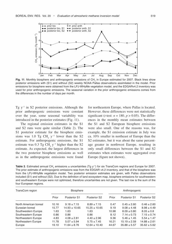
As compared with the prior estimates, posterior estimates of annual biosphere and anthropo-genic emissions for Europe showed reductions (Table 2). The magnitude of the CH4 emission reduction was greater for the biosphere CH4 emissions than for anthropogenic CH4 emissions, whose estimates were reduced from 19.10 to 11.64 (± 8.76) Tg y–1 in S1 and 12.64 (± 10.40) Tg y–1 in S2. The greatest change was seen between June and October for the biosphere CH4 emissions (Fig. 11), which was also illustrated in the comparison of atmospheric mole fractions at Pallas. The estimated anthropogenic CH4 emis-sions for Europe were reduced from 44.67 to 35.88 (± 5.57) Tg y–1 in S1 and 35.62 (± 5.62)

Jan Feb Mar Apr May Jun Jul Aug Sep Oct Nov Dec

–40

–20

0

20

40

xCH

4 (p

pb)

FTIRTM5, priorTM5, S1TM5, S2

Fig. 10. anomalies of monthly Xch4 (column averaged mixing ratios) at sodankylä. Filled circles are monthly means, and the vertical bars are the standard deviations. the Ftir monthly detrended seasonal cycle was calcu-lated from all data from 2009–2012. coloured lines are tm5 estimates for 2007, using monthly prior and weekly posterioremissionfields.Theposterioremissionswereoptimizedassimilatingallglobalflaskmeasurements(S1),and all but the noaa Pallas observations (s2). the nearest observations to sodankylä are from Pallas.


Table 2. estimated annual ch4 emissions ± uncertainties (tg y–1) for six transcom regions and europe for 2007. the prior estimate of anthropogenic emissions was from the eDGar v4.2 inventory, and that of the biosphere was from the lPJ-Whyme vegetation model. two posterior emission estimates are given, with Pallas observations included(S1)andwithout(S2).Duetothedefinitionoflandecosystemmap,biosphereemissionsforsouthwesternand southeastern europe were not optimized, therefore uncertainties are not given. the last row is the sum of the four european regions.

transcom region Biosphere anthropogenic Prior Posterior s1 Posterior s2 Prior Posterior s1 Posterior s2

north american boreal 10.16 9.18 ± 7.15 8.89 ± 7.15 0.47 0.45 ± 2.60 0.46 ± 2.60eurasian boreal 15.77 14.93 ± 10.65 15.25 ± 10.65 9.19 9.08 ± 4.48 8.98 ± 4.49southwestern europe 1.63 1.63 1.63 10.98 8.09 ± 0.80 8.05 ± 0.80southeastern europe 0.86 0.86 0.86 8.12 7.14 ± 0.73 7.15 ± 0.74northwestern europe 4.83 4.08 ± 2.81 4.40 ± 2.96 9.36 5.46 ± 1.45 5.54 ± 1.47northeastern europe 11.78 5.07 ± 5.94 5.75 ± 7.45 16.21 15.19 ± 2.59 14.88 ± 2.61europe 19.10 11.64 ± 8.76 12.64 ± 10.40 44.67 35.88 ± 5.57 35.62 ± 5.62

Jan Feb Mar Apr May Jun Jul Aug Sep Oct Nov Dec0

1

2

3

4

5

6

CH

4 em

issi

on (T

g m

onth

–1)

prior bioposterior bio, S1posterior bio, S2

prior anthposterior anth, S1posterior anth, S2

Fig. 11. monthly biosphere and anthropogenic emissions of ch4 in europe estimated for 2007. Black lines show posterior emissions with (s1) and without (s2) weekly noaa Pallas observations assimilated in the model. Prior emissions for biosphere were obtained from the lPJ-Whyme vegetation model, and the eDGarv4.2 inventory was used for prior anthropogenic emissions. the seasonal variation in the prior anthropogenic emissions comes from the differences in the number of days per month.

Tg y–1 in S2 posterior emissions. Although the prior anthropogenic emissions were constant over the year, some seasonal variability was introduced in the posterior estimates (Fig. 11).

The regional emission estimates in the S1 and S2 runs were quite similar (Table 2). The S1 posterior estimate for the biosphere emis-sions was 1.0 Tg CH4 y--1 lower than the S2 estimate. For anthropogenic emissions, the S1 estimate was 0.3 Tg CH4 y

--1 higher than the S2 estimate. As expected, the largest differences in the two posterior biosphere emissions as well as in the anthropogenic emissions were found

for northeastern Europe, where Pallas is located. However, these differences were not statistically significant (t-test: n = 180, p > 0.05). The differ-ences in the monthly mean estimates between the S1 and S2 European biosphere emissions were also small. One of the reasons was, for example, the S1 emission estimate in July was ca. 10% smaller in northeast of Europe than the S2 estimates, but it was about the same percent-age greater in northwest Europe, resulting in only small differences between the S1 and S2 estimates when estimates were aggregated over Europe (figure not shown).


At high northern latitudes (North American boreal, Eurasian boreal and Europe), our S1 pos-terior estimates for 2007 was 81.16 (± 39.22) Tg CH4 y

–1, which is within the estimated range of Bruhwiler et al. (2014). However, our biosphere emission estimates were more than 10 Tg CH4 y

–1 greater than their estimates, leaving a smaller contribution from the anthropogenic emissions. The biosphere and anthropogenic emissions at high northern latitudes in our S1 estimates were 35.75 (± 26.56) and 45.42 (± 12.65) Tg CH4 y

–1, respectively.

Uncertainties

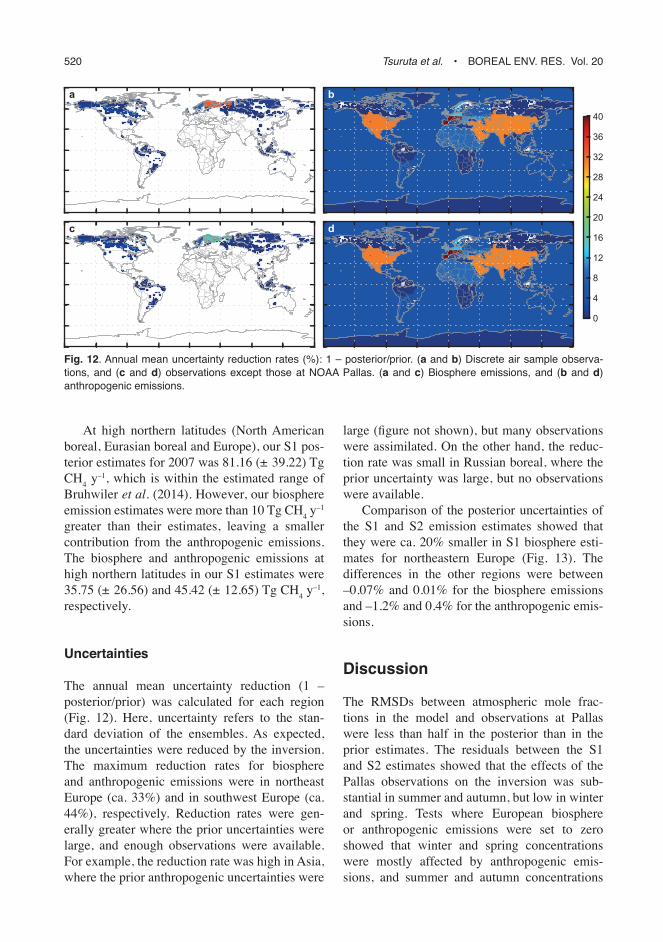
The annual mean uncertainty reduction (1 – posterior/prior) was calculated for each region (Fig. 12). Here, uncertainty refers to the stan-dard deviation of the ensembles. As expected, the uncertainties were reduced by the inversion. The maximum reduction rates for biosphere and anthropogenic emissions were in northeast Europe (ca. 33%) and in southwest Europe (ca. 44%), respectively. Reduction rates were gen-erally greater where the prior uncertainties were large, and enough observations were available. For example, the reduction rate was high in Asia, where the prior anthropogenic uncertainties were

large (figure not shown), but many observations were assimilated. On the other hand, the reduc-tion rate was small in Russian boreal, where the prior uncertainty was large, but no observations were available.

Comparison of the posterior uncertainties of the S1 and S2 emission estimates showed that they were ca. 20% smaller in S1 biosphere esti-mates for northeastern Europe (Fig. 13). The differences in the other regions were between –0.07% and 0.01% for the biosphere emissions and –1.2% and 0.4% for the anthropogenic emis-sions.

Discussion

The RMSDs between atmospheric mole frac-tions in the model and observations at Pallas were less than half in the posterior than in the prior estimates. The residuals between the S1 and S2 estimates showed that the effects of the Pallas observations on the inversion was sub-stantial in summer and autumn, but low in winter and spring. Tests where European biosphere or anthropogenic emissions were set to zero showed that winter and spring concentrations were mostly affected by anthropogenic emis-sions, and summer and autumn concentrations

a b

c d

0

4

8

12

16

20

24

28

32

36

40

Fig. 12. annual mean uncertainty reduction rates (%): 1 – posterior/prior. (a and b) Discrete air sample observa-tions, and (c and d) observations except those at noaa Pallas. (a and c) Biosphere emissions, and (b and d) anthropogenic emissions.


were mainly affected by biosphere emissions. Since Pallas is located in a region of higher sum-mertime biosphere emissions, this confirms the findings of Bruhwiler et al. (2014) that the Pallas observations constrain mostly signals from bio-sphere emissions, and little from the anthropo-genic emissions.

The posterior uncertainties and the error reduction in the S1 and S2 estimates differed most for the biosphere emissions in northeast Europe, where Pallas is located. For other bio-sphere regions and anthropogenic regions, the posterior uncertainties and the reduction rates were almost equal. Thus, the effect of Pallas discrete air sample observations was large in the region where Pallas is located, but small elsewhere. This highlights the ability of the Pallas observations to reduce the uncertainties of biosphere emissions estimates in the region, but they have little influence on the anthropogenic emissions.

The effect of Pallas observations on the column averaged mixing ratios of methane was not as clearly seen as for the surface mixing ratios. The differences between shapes of sea-sonal cycles of S1 and S2 Sodankylä XCH4

estimates were small, although some differ-ences were seen in June and July. There was a decrease in the mean S1 XCH4 from May to June, and an increase from June to July, but the mean S2 XCH4 remained stable from May to June, and decreased from June to July. The monthly changes of S1 match the observations better during the period. The differences between the observations and S1 and S2 estimates were within the estimates by other studies, such as Saito et al. (2012), who estimated a spring model bias of 23.6 ppb. The spring overestimation of the modeled XCH4 in this study may be due to the TM5 model bias in the stratosphere (Alexe et al. 2014, Bergamaschi et al. 2013).

As continuous observations bring a wealth of additional information to constrain the inversion, and may substantially improve the accuracy of optimised emission estimations, we will in our next study use the continuous observations that are available globally.

Furthermore, another useful assessment would be to carry similar tests for other sites. This study suggests that removing Teriberka observations would have little impact on the biosphere emissions, as Pallas observations con-

a

b

–20.0

–17.5

–15.0

–12.5

–10.0

–7.5

–5.0

–2.5

0

Fig. 13. relative differ-ences (%) in the posterior annual mean uncertain-ties are shown for (a) bio-sphere and (b) anthropo-genic emissions between two runs, one with (s1) and another without (s2) noaa Pallas observa-tions assimilated (1 – s1/s2). the negative colours show that the posterior uncertainties were smaller in the s1 estimates.


strain biosphere emissions in northeast Europe well. Also, the differences between S1 and S2 mole fractions at Teriberka suggest that it has little influence on winter anthropogenic emis-sions. Removing all observations from Baltic Sea, Ochsenkopf, and Ocean Station M would influence anthropogenic emission estimates for northern Europe, especially during summer, due to their location, and because Pallas has little influence on summertime anthropogenic emis-sions. However, this study is limited for assess-ing the effects of the Baltic Sea, Ochsenkopf, and Ocean and Zeppelinfjellet observations on surface fluxes in the inversion.

Conclusions

In this study, we explored the ability of European CarbonTracker-CH4, build with the TM5 chem-istry-transport model as an observation oper-ator, to estimate CH

4 emissions in Europe and

boreal region. We specifically looked at the role of the Pallas Station observations by analysing the simulated CH

4 time series with and without

assimilating NOAA Pallas discrete air sample observations. The present analysis shows that European CarbonTracker-CH4 is able to estimate the emissions in northern Finland well. Using optimized emissions, simulated Pallas surface CH4 mole fractions agree well with independent observations. The simulation without Pallas dis-crete air sample observations underestimate pos-terior mole fractions during summer and early autumn. Emission estimates in Europe show that the influence of Pallas discrete air sample observations on uncertainty reduction is larger in European biosphere emissions than in anthropo-genic emissions. The influences in other boreal regions were small. Those indicate that Pallas observations mostly constrain biosphere emis-sions in the European boreal region. This shows that a dense observation network that constrains different emission sources is important for fur-ther development of emission estimates using inverse models. Model performance at other sites and the influence of other observations such as continuous measurements, are an extension of this work to be considered.

Acknowledgements: We thank the Maj and Tor Nessling Foundation, NCoE DEFROST, NCoE eSTICC and the Finn-ish Academy project CARB-ARC (285630) for their finan-cial support. We thank Dr. Akihiko Ito for providing prior emissions of termites. We are grateful for National Institute of Water and Atmospheric Research (NIWA), Laboratoire des Sciences du Climat et de l’Environnement (LSCE), Com-monwealth Scientific and Industrial Research Organisation (CSIRO), Environment Canada (EC), and the Advanced Global Atmospheric Gases Experiment (AGAGE) network for taking discrete air samples at global sites.

References

Aalto T., Hatakka T. & Lallo M. 2007. Tropospheric meth-ane in northern Finland: seasonal variations, transport patterns and correlations with other trace gases. Tellus 59B: 251–259.

Alexe M., Bergamaschi P., Segers A., Detmers R., Butz A., Hasekamp O., Guerlet S., Parker R., Boesch H., Fran-kenberg C., Scheepmaker R.A., Dlugokencky E., Swee-ney C., Wofsy S.C. & Kort E.A. 2014. Inverse modeling of CH4 emissions for 2010–2011 using different satel-lite retrieval products from GOSAT and SCIAMACHY. Atmos. Chem. Phys. Discuss. 14: 11493–11539.

Andreae O. & Merlet P. 2001. Emission of trace gases and aerosols from biomass burning. Global Biogeochem. Cycles 15: 955–966.

Aydin M., Verhulst K.R., Saltzman E.S., Battle M.O., Montzka S.A., Blake D.R., Tang Q. & Prather M.J. 2011. Recent decreases in fossil-fuel emissions of ethane and methane derived from firn air. Nature 476: 198–201.

Bates T.S., Kelly K.C., Johnson J.E. & Gammon R.H. 1996. A reevaluation of the open ocean source of methane to the atmosphere. J. Geophys. Res. 101: 6953–6961.

Bergamaschi P., Krol M., Dentener F., Vermeulen A., Mein-hardt F., Graul R., Ramonet M., Peters W. & Dlugo-kencky E.J. 2005. Inverse modelling of national and European CH4 emissions using the atmospheric zoom model TM5. Atmos. Chem. Phys. 5: 2431–2460.

Bergamaschi P., Frankenberg C., Meirink J.F., Krol M., Dentener F., Wagner T., Platt U., Kaplan J.O., Körner S., Heimann M., Dlugokencky E.J. & Goede A. 2007. Satellite chartography of atmospheric methane from SCIAMACHY on board ENVISAT: 2. Evaluation based on inverse model simulations. J. Geophys. Res. 112, D02304, doi: 10.1029/2006JD007268.

Bergamaschi P., Krol M., Meirink J.F., Dentener F., Segers A., van Aardenne J., Monni S., Vermeulen A.T., Schmidt M., Ramonet M., Yver C., Meinhardt F., Nisbet E.G., Fisher R.E., O’Doherty S. & Dlugokencky E.J. 2010. Inverse modeling of European CH4 emissions 2001–2006. J. Geophys. Res. 115, D22309, doi:10.1029/2010JD014180.

Bergamaschi P., Houweling S., Segers A., Krol M., Fran-kenberg C., Scheepmaker R.A., Dlugokencky E., Wofsy S.C., Kort E.A., Sweeney C., Schuck T., Brenninkmeijer C., Chen H., Beck V. & Gerbig C. 2013. Atmospheric CH4 in the first decade of the 21st century: inverse mod-


eling analysis using SCIAMACHY satellite retrievals and NOAA surface measurements. Atmospheres 118: 7350–7369.

Bousquet P., Hauglustaine D.A., Peylin P., Carouge C. & Ciais P. 2005. Two decades of OH variability as inferred by an inversion of atmospheric transport and chem-istry of methyl chloroform. Atmos. Chem. Phys. 5: 2635–2656.

Bousquet P., Ciais P., Miller J. B., Dlugokencky E.J., Hau-glustaine D.A., Prigent C., Van der Werf G.R., Peylin P., Brunke E.-G., Carouge C., Langenfelds R.L., Lathière J., Papa F., Ramonet M., Schmidt M., Steele L.P., Tyler S.C. & White J. 2011. Contribution of anthropogenic and natural sources to atmospheric methane variability. Nature 443: 439–443.

Brühl C. & Crutzen P.J. 1993. The MPIC 2D Model. NASA reference publication 1292, I: 103–104.

Bruhwiler L.M., Dlugokencky E., Masarie K., Ishizawa M., Andrews A., Miller J., Sweeney C., Tans P. & Worthy D. 2014. CarbonTracker-CH4: an assimilation system for estimating emissions of atmospheric methane. Atmos. Chem. Phys. Discuss. 14: 2175–2233.

Dee D.P., Uppala S.M., Simmons A.J., Berrisford P., Poli P., Kobayashi S., Andrae U., Balmaseda M.A., Balsamo G., Bauer P., Bechtold P., Beljaars A.C.M., van de Berg L., Bidlot J., Bormann N., Delsol C., Dragani R., Fuentes M., Geer A.J., Haimberger L., Healy S.B., Hersbach H., Hólm E.V., Isaksen L., Kållberg P., Köhler M., Matri-cardi M., McNally A.P., Monge-Sanz B.M., Morcrette J.-J., Park B.-K., Peubey C., de Rosnay P., Tavolato C., Thépaut J.-N. & Vitart F. 2011. The ERA-Interim reanal-ysis: configuration and performance of the data assimila-tion system. Q. J. R. Meteorol. Soc. 137: 553–597.

Dentener F. & Bergamaschi P. 2005. The two-way nested global chemistry-transport zoom model TM5: algorithm and applications. Atmos. Chem. Phys. 5: 417–432.

Dlugokencky E.J., Nisbet E.G. & Lowry D. 2011. Global atmospheric methane: budget, changes and dangers. Phil. Trans. R. Soc. A 369: 2058--2072

Dlugokencky E.J., Bruhwiler L., White J.W.C., Emmons L.K., Novelli P.C., Montzka S.A., Masarie K.A., Lang P.M., Crotwell A.M., Miller J.B. & Gatti L.V. 2009. Observational constraints on recent increases in the atmospheric CH4 burden. Geophys. Res. Lett. 36, L18803, doi:10.1029/2009GL039780.

Evensen G. 1994. Sequential data assimilation with a nonlin-ear quasi-Geostrophic model using Monte-Carlo meth-ods to forecast error statistics. J. Geophys. Res. 99: 10143–10162.

Evensen G. 2003. The ensemble Kalman filter: theoretical formulation and practical implementation. Ocean Dyn. 53: 343–367.

Fung I., John J., Lerner J., Matthews E., Prather M., Steele L.P. & Fraser P.J. 1991. Three-dimensional model syn-thesis of the global methane cycle. J. Geophys. Res. 96: 13033–13065.

Fraser P.J., Rasmussen R.A., Creffield J.W., French J.R. & Khalil M.A.K. 1986. Termites and global methane — another assessment. J. Atmos. Chem. 4: 295–310.

Hatakka J., Aalto T., Aaltonen V., Aurela M., Hakola H.,

Komppula M., Laurila T., Lihavainen H., Paatero J., Salminen K. & Viisanen Y. 2003. Overview of the atmo-spheric research activities and results at Pallas GAW station. Boreal Env. Res. 8: 365–383.

Heimann M. 2011. Atmospheric science: Enigma of the recent methane budget. Nature 476: 157–158.

Houweling S., Dentener F.J. & Lelieveld J.1998. The impact of non-methane hydrocarbon compounds tropospheric on photochemistry. J. Geophys. Res. 103: 10673–10696.

Houweling S., Kaminski T., Dentener F., Lelieveld J. & Heimann M. 1999. Inverse modeling of methane sources and sinks using the adjoint of a global transport model. J. Geophys. Res. 104: 26137–26160.

Houweling S., Krol M., Bergamaschi P., Frankenberg C., Dlugokencky E.J., Morino I., Notholt J., Sherlock V., Wunch D., Beck V., Gerbig C., Chen H., Kort E.A., Röckmann T. & Aben I. 2014. A multi-year methane inversion using SCIAMACHY, accounting for system-atic errors using TCCON measurements. Atmos. Chem. Phys. 14: 3991–4012.

Hurtt G.C., Frolking S., Fearon M.G., Moore B., Shevlia-kova E., Malyshev S., Pacala S.W. & Houghton R.A. 2006. The underpinnings of land-use history: three cen-turies of global gridded land-use transitions, wood-har-vest activity, and resulting secondary lands. Global Change Biol. 12: 1–22.

Huttunen J.T., Nykänen H., Turunen J. & Martikainen P.J. 2003. Methane emissions from natural peatlands in the northern boreal zone in Finland, Fennoscandia. Atmos. Environ. 37: 147–151.

IPCC 2013. Climate change 2013: the physical science basis. Working Group I Contribution to the Fifth Assess-ment Report of the Intergovernmental Panel on Cli-mate Change, Cambridge University Press, Cambridge, United Kingdom and New York.

Ito A. & Inatomi M. 2012. Use of a process-based model for assessing the methane budgets of global terrestrial eco-systems and evaluation of uncertainty. Biogeosciences 9: 759–773.

Kai F.M., Tyler S.C., Randerson J.T. & Blake D.R. 2011. Reduced methane growth rate explained by decreased Northern Hemisphere microbial sources. Nature 476: 194–197.

Khalil M.A.K. & Rasmussen R.A. 1985. Causes of increas-ing atmospheric methane: Depletion of hydroxyl radicals and the rise of emissions. Atmos. Environ. 19: 397–407.

Kirschke S., Bousquet P., Ciais P., Saunois M., Canadell J., Dlugokencky E., Bergamaschi P., Bergmann D., Blake D., Bruhwiler L., Cameron-Smith P., Castaldi S., Chevallier F., Feng L., Fraser A., Heimann M., Hodson E., Houweling S., Josse B., Fraser P., Krummel P., Lamarque J.-F., Lagenfelds R., Le Quéré C., Naik V., O’Doherty S.J., Palmer P., Pison I., Plummer D., Poulter B., Prinn R., Rigby M., Ringeval B., Santini M., Schmidt M., Schindell D., Simpson I., Spahni R., Steele P., Strode S., Sudo K., Szopa S., Van der Werf G., Voul-garakis A., van Weele M., Weiss R., Williams J. & Zeng G. 2013. Three decades of global methane sources and sinks. Nat. Geosci. 6: 813–823.

Kivi R., Chen H., Hatakka J., Heikkinen P., Kers B. & Lau-


rila T. 2014. Total column carbon dioxide and methane measurements at Sodankylä. Geophys. Res. Abstracts 16: EGU2014-7969.

Krol M., van Leeuwen P.J. & Lelieveld J. 1998. Global OH trend inferred from methylchloroform measurements. J. Geophys. Res. 103: 10697–10711.

Krol M., Houweling S., Bregman B., van den Broek M., Segers A., van Velthoven P., Peters W., Dentener F. & Bergamaschi P. 2005. The two-way nested global chem-istry-transport zoom model TM5: algorithm and applica-tions. Atmos. Chem. Phys. 5: 417–432.

Langenfelds R.L., Francey R.J., Pak B.C., Steele L.P., Lloyd J., Trudinger M. & Allison C.E. 2002. Interannual growth rate variations of atmospheric CO2 and its δ13C, H2, CH4, and CO between 1992 and 1999 linked to bio-mass burning. Global Biogeochem. Cycles 16(3), 1048, doi:10.1029/2001GB001466.

Locatelli R., Bousquet P., Chevallier F., Fortems-Cheney A., Szopa S., Saunois M., Agusti-Panareda A., Bergmann D., Bian H., Cameron-Smith P., Chipperfield M.P., Gloor E., Houweling S., Kawa S.R., Krol M., Patra P.K., Prinn R.G., Rigby M., Saito R. & Wilson C. 2013. Impact of transport model errors on the global and regional meth-ane emissions estimated by inverse modelling. Atmos. Chem. Phys. 13: 9917–9937.

MacFarling Meure C., Etheridge D., Trudinger C., Steele P., Langenfelds R., van Ommen T., Smith A. & Elkins J. 2006. Law Dome CO2, CH4 and N2O ice core records extended to 2000 years BP. Geophys. Res. Lett. 33, L14810, doi:10.1029/2006GL026152.

Matthews E. & Fung I. 1987. Methane emission from natural wetlands: global distribution, area, and environmental characteristics of sources. Global Biogeochem. Cycles 1: 61–86.

Monteil G., Houweling S., Dlugockenky E.J., Maenhout G., Vaughn B.H., White J.W.C. & Rockmann T. 2011. Inter-preting methane variations in the past two decades using measurements of CH

4 mixing ratio and isotopic compo-

sition. Atmos. Chem. Phys. 11: 9141–9153.Peters W., Miller J.B., Whitaker J., Denning A.S., Hirsch

A., Krol M.C., Zupanski D., Bruhwiler L. & Tans P.P. 2005. An ensemble data assimilation system to estimate CO2 surface fluxes from atmospheric trace gas observations. J. Geophys. Res. 110, D24304, doi:10.1029/2005JD006157.

Peters W., Jacobson A.R., Sweeney C., Andrews A.E., Conway T.J., Masarie K., Miller J.B., Bruhwiler L.M.P., Petron G., Hirsch A.I., Worthy D.E.J., van der Werf G.R., Randerson J.T., Wennberg P.O., Krol M.C. & Tans P.P. 2007. An atmospheric perspective on North Amer-ican carbon dioxide exchange: CarbonTracker. Proc. Natl. Acad. Sci. USA 104: 18925–18930.

Peters W., Krol M.C., van der Werf G.R., Houweling S., Jones C.D., Hughes J., Schaefer K., Masarie K.A., Jacobson A.R., Miller J.B., Cho C.H., Ramonet M., Schmidt M., Ciattaglia L., Apadula F., Heltai D., Mein-hardt F., Di Sarra A.G., Piacentino S., Sferlazzo D., Aalto T., Hatakka J., Ström J., Haszpra L., Meijer H.A.J., van der Laan S., Neubert R.E.M., Jordan A., Rodó X., Morguí J.-A., Vermeulen A.T., Popa E., Rozanski K.,

Zimnoch M., Manning A.C., Leuenberger M., Uglietti C., Dolman A.J., Ciais P., Heimann M. & Tans P.P. 2010. Seven years of recent European net terrestrial carbon dioxide exchange constrained by atmospheric observa-tions. Global Change Biol. 16: 1317–1337.

Prigent C., Papa F., Aires F., Rossow W.B. & Matthews E. 2007. Global inundation dynamics inferred from multi-ple satellite observations, 1993–2000. J. Geophys. Res. 112, D12107, doi:10.1029/2006JD007847.

Prinn R.G., Weiss R.F., Fraser P.J., Simmonds P.G., Cunnold D.M., Alyea F.N., O’Doherty S., Salameh P., Miller B.R., Huang J., Wang R.H.J., Hartley D.E., Harth C., Steele L.P., Sturrock G., Midgely P.M. & McCulloch A. 2000. A history of chemically and radiatively important gases in air deduced from ALE/GAGE/AGAGE. J. Geo-phys. Res. 115: 17751–17792.

Rasmussen R.A. & Khalil M.A.K. 1981. Atmospheric meth-ane (CH4): Trends and seasonal cycles. J. Geophys. Res. 86: 9826–9832.

Rhodes R.H., Faın X., Stowasser C., Blunier T., Chappellaz J., McConnell J.R., Romanini D., Mitchell L.E. & Brook E.J. 2013. Continuous methane measurements from a late Holocene Greenland ice core: atmospheric and in-situ signals. Earth Plan. Sci. Lett. 386: 9–19.

Rigby M., Prinn R.G., Fraser P.J., Simmonds P.G., Lan-genfelds R.L., Huang J., Cunnold D.M., Steele L.P., Krummel P.B., Weiss R.F., O’Doherty S., Salameh P.K., Wang H.J., Harth C.M., Mühle J. & Porter L.W. 2008. Renewed growth of atmospheric methane. Geophys. Res. Lett. 35, L22805, doi:10.1029/2008GL036037.

Saarnio S., Winiwarter W. & Leitao J. 2009. Methane release from wetlands and watercourses in Europe. Atmos. Envi-ron. 43: 1421–1429.

Saito R., Patra P.K., Deutscher N., Wunch D., Ishijima K., Sherlock V., Blumenstock T., Dohe S., Griffith D., Hase F., Heikkinen P., Kyrä E., Macatangay R., Mendonca J., Messerschmidt J., Morino I., Notholt J., Rettinger M., Strong K., Sussmann R. & Warneke T. 2012. Techni-cal Note: Latitude-time variations of atmospheric col-umn-average dry air mole fractions of CO2, CH4 and N2O. Atmos. Chem. Phys. 12: 7767–7777.

Sonnemann G.R. & Grygalashvyly M. 2014. Global annual methane emission rate derived from its current atmo-spheric mixing ratio and estimated lifetime. Ann. Geo-phys. 32: 277–283.

Spahni R., Wania R., Neef L., van Weele M., Pison I., Bousquet P., Frankenberg C., Foster P.N., Joos F., Pren-tice I.C. & van Velthoven P. 2011. Constraining global methane emissions and uptake by ecosystems. Biogeo-sciences 8: 1643–1665.

Spivakovsky C.M., Logan J.A., Montzka S.A., Balkanski Y.J., Foreman-Fowler M., Jones D.B.A., Horowitz L.W., Fusco A.C., Brenninkmeijer C.A.M., Prather M.J., Wofsy S.C. & McElroy M.B. 2000. Three-dimensional climatological distribution of tropospheric OH: update and evaluation. J. Geophys. Res. 105: 8931–8980.

van der Werf G.R., Randerson J.T., Giglio L., Collatz G.J., Mu M., Kasibhatla P.S., Morton D.C., DeFries R.S., Jin Y. & van Leeuwen T.T. 2010. Global fire emissions and the contribution of deforestation, savanna, forest, agri-


cultural, and peat fires (1997–2009). Atmos. Chem. Phys. 10: 11707–11735.

Villani M.G., Bergamaschi P., Krol M., Meirink J.F. & Den-tener F. 2010. Inverse modeling of European CH4 emis-sions: sensitivity to the observational network. Atmos. Chem. Phys. 10: 1249–1267.

Wania R., Ross I. & Prentice I.C. 2010. Implementation and evaluation of a new methane model within a dynamic global vegetation model: LPJ-WHyMe v1.3. Geosci. Model Dev. Discuss. 3: 1–59.

Wanninkhof R. 1992. Relationship between wind speed and gas exchange over the ocean. J. Geophys. Res. 97: 7373–7382.

Wiesenburg D.A. & Guinasso N.L.Jr. 1979. Equilibrium solubilities of methane, carbon monoxide, and hydrogen in water and sea water. J. Chem. Eng. Data 24: 356–360.

Wunch D., Wennberg P.O., Toon G.C., Connor B.J., Fisher

B., Osterman G.B., Frankenberg C., Mandrake L., O’Dell C.W., Ahonen P., Biraud S.C., Castano R., Cres-sie N., Crisp D., Deutscher N.M., Eldering A., Fisher M.L., Griffith D.W.T., Gunson M., Heikkinen P., Kep-pel-Aleks G., Kyrö E., Lindenmaier R., Macatangay R., Mendonca J., Messerschmidt J., Miller C.E., Morino I., Notholt J., Oyafuso F.A., Rettinger M., Robinson J., Roehl C.M., Salawitch R.J., Sherlock V., Strong K., Sussmann R., Tanaka T., Thompson D.R., Uchino O., Warneke T. & Wofsy S.C. 2011. A method for evaluating bias in global measurements of CO2 total columns from space, Atmos. Chem. Phys. 11: 12317–12337.

Yvon-Durocher G., Allen A.P., Bastviken D., Conrad R., Gudasz C., St-Pierre A., Thanh-Duc N. & del Giorgio P.A. 2014. Methane fluxes show consistent tempera-ture dependence across microbial to ecosystem scales. Nature 507: 488–491.

Documents

evaluating atmospheric methane inversion model results for