Embed Size (px)
Citation preview

European Economic Review 135 (2021) 103718
Contents lists available at ScienceDirect
European Economic Review
journal homepage: www.elsevier.com/locate/euroecorev
Corporate governance and industrialization !
Maurizio Iacopetta a , Pietro F. Peretto b , ∗
a SKEMA Business School, Université Côte d’Azur (GREDEG) and OFCE Sciences Po, France b Duke University, United States
a r t i c l e i n f o
Article history: Received 22 January 2021 Revised 5 March 2021 Accepted 20 March 2021 Available online 3 April 2021
JEL classification: D58 O14 O16 O43 O57
Keywords: Corporate governance Income differences Secular transition Modern growth
a b s t r a c t
Corporate governance distortions delay or even halt a country’s transformation into a mod- ern innovation economy. We investigate the mechanism through a growth model that al- lows for agency issues within firms. Governance distortions raise the cost of investment and depress the incentives to set up new firms. Modest differences in governance account for large gaps in income: A 32 percent investment cost differential can explain the secular decline of Latin America income relative to that of the USA, and implies an industrializa- tion delay of a third of a century. We obtain similar results for a large number of countries and macro-regions.
© 2021 Elsevier B.V. All rights reserved.
1. Introduction
Corporate innovation is a major driver of modern growth. The centrality of the corporation in the growth process, how-
ever, is relatively recent. In Prussia in the middle of the 19th century, Ernst Werner Siemens started up what would become
one of the world’s largest manufacturing and innovative company. In the USA in the second half of the 19th century, Thomas
Edison established one of the most prolific industrial research and development lab, whose operations were closely related
to his manufacturing enterprises. Similar undertakings occurred in several industries, giving birth to companies such as
General Electric, AT&T and General Motors, to name a few, that are still thriving today. This cluster of events marks a pro-
found qualitative change in the mode of growth. First, the rise of the innovative corporation brings to the forefront issues
! We thank for useful comments Philippe Aghion, Angus Chu, Antonio Fatas, Domenico Ferraro, Elie Gray, Giammario Impullitti, David Le Bris, Florencio Lopez de Silanes, Rafael Matta, Raoul Minetti, and participants at the 2020 Virtual Meetings of the Econometric Society, 2019 Conference of Georgetown Center of Economic Research, Washington DC, the 10th IBEO Conference, Alghero, the Growth and Structural Change Workshop, Toulouse Business School, the 2019 Royal Economic Society Annual Conference, Warwick, the INSEAD Economics and Political Science Seminar Series (Fontainebleau, Singapore, and Abu Dhabi), Duke University Macro Seminar Series, the 2017 Workshop “Innovation, Economic Growth and Corporate Governance” (OFCE-SKEMA Business School), the Conference on ”Finance and Economic Growth After the Crisis,” University of Milan, the 2017 Meetings of the French Economic Association (Nice, France), the Meetings of the Southern Economic Association (Tampa, Florida, USA), the Zhejiang University Economics Seminar Series (Hangzhou, China), the NAU-IUD Innovation Economics Workshop (Nanjing, China). All remaining errors are ours.
∗ Corresponding author. E-mail addresses: [email protected] (M. Iacopetta), [email protected] (P.F. Peretto).
https://doi.org/10.1016/j.euroecorev.2021.103718 0014-2921/© 2021 Elsevier B.V. All rights reserved.

M. Iacopetta and P.F. Peretto European Economic Review 135 (2021) 103718
Fig. 1. Governance and Delays in Industrialization Note: Data source : Maddison Database (2010) and Rule of Law, Estimate of Governance, 2017, World Bank (see Kaufmann et al., 2010 ). Period 1 : 1770–1820; Period 2 : 1820–1870; Period 3 : 1870–1900; Period 4 : 1900–1950; Period 5: 1950-1975; Period 6 : 1975–1990; Period 7 : 1990–2008; Take-offs (countries ordered within each group according to per capita income in 2008). Period 1 : USA; Period 2 : Norway, Ireland, Australia, Canada, Switzerland, Netherlands, Denmark, Sweden, Finland, Austria, United Kingdom, Belgium, France, Germany, New Zealand, Chile, Argentina, Uruguay, Tunisia, Sri Lanka, South Africa, and Algeria. Period 3 : Japan, Trinidad and Tobago, Estonia, Spain, Slovenia, Greece, Puerto Rico, Latvia, Portugal, Slovak Republic, Czech Republic, Belarus, Armenia, Kazakhstan, Venezuela, Poland, Hungary, Russian Feder., Croatia, Bulgaria, Azerbaijan, Costa Rica, Mexico, Bosnia and Herz., Panama, Colombia, Georgia, Uzbekistan, Ukraine, Romania, Dominican Repub., Guatemala, Turkmenistan, Albania, Macedonia, Ecuador, Cuba, Jamaica, Serbia, Moldova, Paraguay, Vietnam, Bolivia, El Salvador, Kyrgyz Republic, Honduras, Nicaragua, Ghana, Tajikistan, Nepal, and Haiti; Period 4 : Hong Kong, Singapore, China, Taiwan, Italy, Israel, Qatar, United Arab Emirates, Mauritius, Kuwait, Malaysia, Saudi Arabia, Syria, Turkey, Bahrain, Iran, Brazil, Seychelles, Jordan, Peru, Namibia, Lebanon, Gabon, Egypt, Morocco, Philippines, Yemen, West Bank and Gaza, Mozambique, Rep. of Congo, Angola, Senegal, Benin, Djibouti, Côte d’Ivoire, Iraq, Somalia, Liberia, and Madagascar; Period 5 : Equatorial Guinea, Thailand, Oman, China, Botswana, Indonesia, Swaziland, Libya, India, Cambodia, Pakistan, Lesotho, Laos, Nigeria, São Tomé and Principe, Mauritania, Cameroon, Mali, Kenya, Burkina Faso, The, Gambia, Rwanda, Mongolia, Eritrea, Zambia, Zimbabwe, Tanzania, Malawi, Sierra Leone, Guinea, Guinea-Bissau, Togo, Comoros, Burundi, Congo (Dem. Rep.); Period 6 : Cape Verde and Bangladesh; Period 7 : Sudan, Uganda, Afghanistan, and Chad; No take-off resulted for Niger and Central African Republic.
of corporate governance due to separation of ownership from control, and more generally misalignment of interests among
stakeholders, that in previous times where not as salient. Second, the increasing importance of corporate innovation ac-
celerated the process of divergence of different communities (provinces, regions, countries). Fig. 1 reports the first growth
acceleration for 155 countries. For 22 of these countries it occurred sometimes between 1820 and 1870 and for 51, 38 and
35 countries in, respectively, the 1870–1900, 1900–1950 and 1950–1975 periods. 1 Fig. 1 also correlates the countries’ growth
accelerations with the Rule of Law score, which, of the six World Bank Worldwide Governance Indicators, is the one that
measures how confident people are in property rights, contract enforcement and the quality of courts — arguably essen-
tial ingredients of good corporate governance. 2 The pattern suggests that industrialization delays are considerably longer in
countries that have a low governance score.
To explore the role of corporate governance in the determination of such pattern, we integrate corporate governance
distortions due to principal-agent problems in a model where growth is driven by investments of incumbent firms and
entry of new firms. We characterize the rise of the industrial economy as the acceleration of the rate of formation of new
firms that market new intermediate inputs and the intensification of firms’ in-house knowledge accumulation. We use the
1 We consider growth acceleration a period characterized by an annual average growth rate of per capita income of at least 0.72%; this corresponds to that of the USA in the period 1700–1820 (period 1). This is lower than the 2% threshold employed by Hausmann et al. (2005) who, however, are interested in episodes of post-WWII growth spurts.
2 For instance, in a review of 67 countries ( Doidge et al., 2007 ) find that where the rule of law is stronger, the resulting lower agency costs allow firms to take better advantage of growth opportunities.
2

M. Iacopetta and P.F. Peretto European Economic Review 135 (2021) 103718
model to evaluate how corporate governance distortions affect the growth of the individual firm, the evolution of industry,
the timing of the economy’s transition to modern growth and thereby the secular path of national income.
In the model, the source of corporate governance distortions is the ability of managers to divert the firm’s resources to
private benefits; see, among others, Nikolov and Whited (2014) and Shleifer and Wolfenzon (2002) . Specifically, managers
divert cash flow and planned investment funds to their own consumption. The former reduces the distribution of dividends
to shareholders and has first-order effects on the incentive to set up firms. The latter raises the cost of investing in the
growth of the firm. Shareholders can partially discipline managers through incentive compensation contracts and by hiring
monitoring agents (e.g., directors).
The economy starts with a given number of firms. Initially, market expansion fueled by population growth is the only
source of income growth via Smithian economies of scale. Under some conditions, such market expansion eventually triggers
entry of new firms and, later, in-house investment by incumbent firms. The timing of the two events has long-lasting con-
sequences for the path of income per capita. We investigate how the governance structure of firms, an equilibrium outcome
of our analysis, affects the macroeconomic equilibrium and results in different histories. Because both the rate of entry and
the rate of in-house innovation rise as the economy converges to its steady state, an economy with more severe corporate
governance distortions enters the modern growth phase later and exhibits poorer productivity performance throughout the
transition. In this sense, the timing of the take-off ”imprints” on the whole subsequent evolution of the economy.
To assess how well corporate governance accounts quantitatively for the observed cross-country income dynamics, we
calibrate the model to the USA for the period 170 0–20 08, taking 180 0 as the beginning of modern growth (see, among others
( Lucas, 20 0 0 ) and assuming the USA to be at a 10% distance from a distortion-free economy (see Iacopetta et al., 2019 ). Using
the USA as a benchmark, we then calculate how over the same period variations in corporate governance explain the timing
of the transition to modern growth and the performance afterwards of several other countries and some macro regions.
The key to this exercise is that, differently from the USA, we let the model determine endogenously the take-off date for
these units. We find, for instance, that the magnitude of the difference in corporate governance distortions to account for
the decline of the income per capita of Latin America relative to the USA, from one to one fourth, is the equivalent of a 32
percent higher cost of in-house investment in Latin America. We also calculate that such a distortion delays modern growth
by approximately a third of a century, a delay that accounts well for the end-of-period (2008) income gap.
To validate the model, we perform three types of tests under the assumption that the institutional environment stays the
same over the three centuries. The first test correlates the two endogenous variables of the model that represent corporate
governance distortions, the shareholders appropriation factor ( a ) and the in-house cost of innovation ( q ), with the World
Bank rule of law index. In both cases the correlation is strong and of the right sign. The two variables a and q are central to
our analysis because they determine the economy’s waiting times before the transitions to the variety expansion and quality
innovation phases of development. The second test compares the model-predicted take-off dates to the timing of the first
growth accelerations shown in Fig. 1 . The agreement between model’s prediction and data for the countries that started
growing in the 19th century is quite strong. The model, however, tends to underestimate the take-off dates of countries,
like Japan and China, that started growing in the 20th century and went through very rapid growth accelerations. The
third test compares the model-generated time series of per capita income of individual countries to the Maddison data.
The model fits the data remarkably well for today’s rich economies and the large Latin America economies. There are,
in contrast, visible deviations between model and data for fast growing Asian countries: the model underestimates the
date of the first acceleration and the steepness of the subsequent growth path of these countries. However, once we allow
the quality of governance to improve in the post-war period, due to underlying institutional changes, we find that the
model fits the data better for these countries but not that for Western economies. This result suggests that, under the
assumption of stable corporate governance, the model fails precisely where it should because it neglects, for example, the
drastic institutional transformation of Japan after WWII and the reforms in China in the 80s that unshackled the economies
of those two countries.
Our paper contributes to the large literature that attributes the fortunes of modern economies to the process of creation
of technical knowledge ( Chu et al., 2014; Peretto, 2015; Chu et al., 2019; Madsen et al., 2019 ). Like this literature, we stress
that take-off events are accelerations of income growth along the transition to the modern innovation-economy stage. How-
ever, we expand the perspective to new dimensions because we focus on corporate governance and on the arrival on the
scene of the Schumpeterian innovative firm.
Similarly, the paper contributes to the literature that links corporate governance to macroeconomic performance and
that, more specifically, investigates the long-run implications for aggregate productivity and welfare of within-firm con-
tractual frictions and of financial markets imperfections; see, e.g., Celik and Tian (2019) , Iacopetta et al. (2019) , Lopez and
Vives (2019) , Terry (2017) , Aghion et al. (2005) , Cooley and Quadrini (2001) .
While the analytical framework that we use is similar to that of Iacopetta et al. (2019) , here we expand the perspective
in three dimensions. 3 First, we consider both advanced countries and countries at earlier stages of the process of secular
growth and transformation. In particular, we account for the phase transitions that bring about the key qualitative changes in
the structure of the economy, including the internal structure of firms. Second, we allow for misuse not only of cash but also
3 Iacopetta et al. (2019) studies the effects of managers’ ability to (a) divert the firm’s cash flow to private benefits and (b) nurture their empire bulding ambitions. The focus is on advanced economies and local dynamics around the balanced-growth steady state.
3

M. Iacopetta and P.F. Peretto European Economic Review 135 (2021) 103718
of planned investment. This type of diversion has acquired prominence in the literature recently. Terry (2017) , for example,
argues that managers’ ability to divert investment funds to short-term objectives have important ramifications for macroe-
conomic performance. Third, we postulate a board of directors that supervise the manager, following recent developments in
the financial literature (Page 2018, Balsmeier et al. (2016) ) that stress the importance of monitoring for good corporate gov-
ernance. Celik and Tian (2019) , in particular, provide evidence that directors discipline executive officers through incentives
and supervision. 4
Aside from the differences in the description of the firm’s agency issues and the presence of internal monitoring, the
main aspect that differentiates this work from Iacopetta et al. (2019) is that ( Iacopetta et al., 2019 ) studied the economy’s
deviation from the steady state in response to shocks to the rule of law, keeping constant the structure of corporate gov-
ernance, while here we focus on (i) global dynamics, (ii) the qualitative differences in corporate governance across devel-
opment phases and (iii) how the take-off times are linked to corporate governance. One crucial property of the analysis
is that the strong convexity of the income path—the dramatic growth acceleration that is the essence of industrialization—amplifies massively the effects of delays in crossing the two thresholds of firm size marking the different phases. Specifically,
our quantitative experiments suggest that small distortions in q and a account for the large gaps at the end of the income
time series. Differently from most of the literature on macro-development, in our paper institutions operate through the in-
ternal governance of the firm—a transmission and propagation channel distinctive of our modeling approach. To summarize,
the added elements relative to Iacopetta et al. (2019) —diversion of planned investment, board of directors with expand-
ing span of monitoring tasks—allow us to develop a theory that puts corporate governance at the heart of the process of
industrialization and convergence to modern growth. In particular, they allow us to (i) endogenize specific, important di-
mensions of corporate governance ( Section 3.6 and ( Proposition 2 ), (ii) show how they evolve through the phases of the
process ( Section 5 ), and ((iii) estimate the magnitude of relative distortions across countries from income data ( Section 6 ).
More broadly, our analysis complements the literature that investigates how institutions, the government as well as le-
gal and social norms, drive cross-country income differences. Several scholars argue that in Western Europe the rule of
law was already taking hold in the Middle Ages, while in other regions it developed much later and in some it never
did. In other words, the conditions for the formation of the modern innovative firm emerged unevenly around the world.
In places where the rule of law was not sufficiently advanced, business communities developed alternative arrangements
based on trust that allowed production and commerce to thrive ( Greif, 2006 ). Trust is a powerful ingredient in promoting
investment because even in a sophisticated contractual environment a party’s future choice is not necessarily contractible
( Lins et al., 2017 ), ( Fukuyama, 2014 ). Augmenting this historical perspective, there is now established evidence that corpo-
rate governance affects the investment of incumbent firms and the formation of new firms; see, e.g., Aghion et al. (2013) ,
Morck et al. (2005) and Fulghieri and Suominen (2012) . Most importantly, such evidence highlights differences across coun-
tries in corporate governance due to differences in the local institutional environments.
The paper is organized as follows. Section 2 reviews the basic growth model. Section 3 augments the model with corpo-
rate governance and derives the main microeconomic results. Sections 4 and 5 develop the macroeconomic implications of
corporate governance. Section 6 calibrates the model and performs several quantitative exercises. Section 7 evaluates the fit
of the model to the data. Section 8 concludes.
2. The basic growth model
The model builds on the literature that integrates endogenous market structure in the theory of economic growth. The
framework provides a natural way to exploit insights from Industrial Organization to understand how corporate governance
frictions affect innovation-driven growth. In this section we set up the model abstracting from frictions, which we introduce
later. Time is continuous and infinite. All variables are functions of time but to simplify the notation we omit the time ar-
gument unless necessary to avoid confusion. The economy is closed. The production side consists of a final sector producing
a homogeneous good and an intermediate sector producing a continuum of differentiated non-durable goods.
2.1. Final producers
A competitive representative firm produces a final good that can be consumed, used to produce intermediate goods,
invested in the improvement of the quality of existing intermediate goods, or invested in the creation of new intermediate
goods. The final good is our numeraire. The production technology is
Y =
∫ N
0 X θi
(Q i L
γi #
1 −γ)1 −θ
di, 0 < θ , γ < 1 (1)
where N is the mass of non-durable intermediate goods and L i and # are, respectively, services of labor and a fixed factor
(e.g., land). The parameters θ and γ govern the output elasticity to intermediate inputs and to labor, respectively. The
4 Our concept of stealing-monitoring Nash Equilibrium, developed formally in Section 3 , complements the Celik-Tian approach and extends the perspec- tive on the interaction between executives and directors. They postulate a board that makes decisions subject to CEO influence, which they capture in reduced from with a parameter representing the weight of the CEO’s preferences in the board’s maximization problem. We postulate direct strategic in- teraction between directors and executives in specific dimensions of the firm’s oparations. The two approaches are complementary and suggest that future work will likely develop a comprehensive characterization of corporate governance embedded in dynamic macroeconomic models.
4

M. Iacopetta and P.F. Peretto European Economic Review 135 (2021) 103718
technology features dilution of labor across intermediate goods, reflecting the property that both labor and intermediate
goods are rival inputs. The fixed factor is non-rival across labor and intermediate products. Quality, Q i , is the good’s ability
to raise the productivity of the other factors. Let P i be the price of intermediate good i, w the wage and p the price of the
fixed factor. The profit maximization problem yields that the final producer demands each intermediate good according to
X i =
(θP i
) 1 1 −θ
Q i L γi #
1 −γ . (2)
Moreover, the final producer pays
∫ N
0 P i X i di = θY, wL =
∫ N
0 wL i di = γ ( 1 − θ ) Y, p# = ( 1 − γ ) ( 1 − θ ) Y (3)
to, respectively, suppliers of intermediate goods, labor and the fixed factor.
2.2. Intermediate producers
In line with Schumpeterian theory, we view firms as complex organizations that develop and apply specialized knowl-
edge. Therefore, we model quality as
Q i = Z αi Z 1 −α . (4)
In words, the contribution of good i to factor productivity downstream depends on the knowledge of firm i, Z i , and on
average knowledge, Z = ∫ N
0
(Z j /N
)dj. The firm requires one unit of final output per unit of intermediate good produced and
a fixed operating cost, φZ αi Z 1 −α, also in units of final output. The firm accumulates knowledge according to
˙ Z i = I i , (5)
where I i is in-house investment in units of final good. Using (2) and (4) , we write the firm’s gross cash flow (revenues minus
production costs) as
F i ≡ ( P i − 1 ) X i − φQ i =
[
( P i − 1 )
(θP i
) 1 1 −θ
L γi #
1 −γ − φ
]
Z αi Z 1 −α . (6)
In this expression α is the elasticity of the firm’s gross cash flow with respect to its own knowledge. The dividend flow is
&i = F i − I i and the value of the firm is
V i ( t ) =
∫ ∞
t e −
∫ τt r ( v ) dv &i (τ ) dτ . (7)
Creating a new firm costs βX units of final output, where X = ∫ N
0 ( X i /N ) di is average intermediate output. The resulting free-
entry condition is V i = βX . Because of this sunk entry cost, the new firm cannot supply an already existing good in Bertrand
competition with the incumbent monopolist but introduces a new intermediate good that expands product variety. The
firm enters at the average knowledge level and hence at average size (this simplifying assumption preserves symmetry of
equilibrium at all times, see below).
2.3. Households
The economy is populated by a representative household with L ( t ) = L 0 e λt , L 0 ≡ 1 , members, each endowed with one
unit of labor. The household has preferences
U ( t ) =
∫ ∞
t e −( ρ−λ) ( τ−t ) log
(C ( τ )
L ( τ )
)dτ, ρ > λ ≥ 0 (8)
where t is the point in time when the household makes decisions, ρ is the discount rate and C is consumption. The house-
hold supplies labor inelastically and has budget constraint
˙ A = rA + wL + p# − C, (9)
where A is assets holding and r is the rate of return on assets. The intertemporal consumption plan that maximizes (8) sub-
ject to (9) consists of the Euler equation
r = ρ − λ + ˙ C /C, (10)
the budget constraint (9) and the usual boundary conditions.
5

M. Iacopetta and P.F. Peretto European Economic Review 135 (2021) 103718
3. Corporate governance
We now allow for frictions arising from separation of ownership and control. The literature describes managers as indi-
viduals who pursue personal goals rather than shareholder value. To capture such a misalignment of interests, we focus on
two flows of resources that managers can divert to personal gain: cash flow and planned investment.
3.1. Governance: set up
Our typical firm has three constituencies with different interests. The first consists of individuals who supply the re-
sources to set up the firm. For convenience we refer to this group in the singular as the founder . 5 His objective is to maxi-
mize the value of the firm. The second constituency is the firm’s management. We refer to this group as the manager . The
third constituency, which we call the director , consists of individuals who monitor the managers’ activities. The manager’s
and the director’s objectives are to maximize their own utility.
The governance scheme is the following. The founder hires the manager, to whom he delegates production and pricing
decisions and the implementation of the investment plan, and the director, to whom he delegates monitoring the manager.
The founder formulates the investment plan, which specifies a time path of expenditure on product quality improvement.
Misalignment of interests arises because the manager can divert planned investment funds and/or cash flow to his own
private benefit. We consider two devices at the founder’s disposal to control such moral hazard. The first is hiring the
director, who can reduce directly the manager’s ability to divert resources. The second is the compensation package: the
founder offers a contract that grants remuneration tied to the firm’s increment of the stock of knowledge (actual investment)
and to the cash flow available for dividend distribution (actual cash flow or the cash flow net of diversion). 6
The assumption that the founder formulates the investment plan while the manager only executes it might seem re-
strictive. It is nevertheless convenient in our contest for two reasons. First, it allows us to emphasize that even when the
manager controls only routine operations his actions may harm the interests of shareholders. Second, it makes the formal
analysis simpler and much more transparent than the alternative of letting the manager formulate the investment plan.
Indeed, precisely because the founder proposes a compensation package and maintains control of the investment plan, we
can see within a coherent dynamic optimization problem the interaction between the compensation package decision and
the investment choice.
To summarize, at the foundation of the firm, the principal, our founder, makes three decisions. First, he hires two agents,
the manager and the director, offering compensation that takes into account their incentives and constraints. Second, he
specifies the investment plan with full understanding that there will be a wedge between planned and actual investment.
Third, he decides whether to set up the firm, with full understanding that there will be a wedge between the profit gener-
ated by the firm and what he receives as dividend.
3.2. Manager (agent)
The manager can divert a share S F i
(M F
i , D F i ;+
)of cash flow, F i , at utility cost c F
M (M F i ;+) · F i . The share S F
i
(M F
i , D F i ;+
)is
increasing in the manager’s effort M F i and decreasing in the director’s effort D F
i . The function c F M (M F
i ;+) is increasing in M F i .
The manager can also divert a share S I i
(M I
i , D I i ;+
)of planned investment, I i , at utility cost c I
M (M I i ;+) · I i , where the functions
S I i ( . ) and c I
M (. ) have the same properties as the functions S F i ( . ) and c F
M (. ) , and M I i and D I
i are, respectively, the manager’s
and the director’s efforts. Actual investment is thus
˙ Z i = [1 − S I
i
(M I
i , D I i ;+
)]· I i . (11)
The term + denotes the set of parameters that govern the cost-benefit calculations of our agents through the functions
described above and thus connects the model’s micro structure to the concept of ”quality of institutions” discussed in the
introduction. Specifically, measures like the World Bank Rule of Law score combine a variety of elements of a country’s
institutional, social and cultural environment into a single number that is then used as a summary statistic of the country’s
”quality of institutions”. Our analytical structure proposes that such multiple dimensions manifest themselves as country-
specific costs and benefits faced by principal and agents and thereby determine the internal governance of the firm. For
concreteness, henceforth we refer to + as the ”institutional environment”. 7 Considering two types of diversion effort s, one
targeted at cash flow and the other at planned investment, allows the emergence of different corporate governance struc-
tures across institutional environments and depending on the size of the firm (more on this in Section 5 ).
5 While each of the constituencies is typically a plurality of individuals, possibly with different preferences and constraints, it is easier to describe the setup assuming homogeneity within each group.
6 To keep the exposition simple we use only contracts that compensate the manager and the director in proportion to the resources subject to diversion. Other schemes are possible, of course, but they complicate matters without necessarily adding insight.
7 Because it contains the parameters of the utility cost of diversion, our concept of institutional environment is quite broad and allows not only for things like the importance of the rule of law, the expectations that contracts are secure because enforced by the courts, opacity in accounting that makes diversion of funds easier, but also things like cultural and social stigma toward cheating and self-restraint driven by the individual internalization of similar cutural and social norms.
6

M. Iacopetta and P.F. Peretto European Economic Review 135 (2021) 103718
The manager’s contract specifies as compensation fractions m I i and m F
i of the resources that he can divert. The manager
fully consumes his income and thus his utility flow is
u manager i =
{m F
i
[1 − S F
i
(M F
i , D F i ;+
)]+
[S F
i
(M F
i , D F i ;+
)− c F
M (M F i ;+)
]}F i
+ {
m I i
[1 − S I
i
(M I
i , D I i ;+
)]+
[S I
i
(M I
i , D I i ;+
)− c I
M (M I i ;+)
]}I i .
At time t, he chooses for τ ∈ [ t, ∞ ) the paths of price, P i (τ ) , and effort s, M F i ( τ ) , M I
i ( τ ) , that, given the paths of m F i ( τ ) and
m I i ( τ ) , maximize
V manager
i ( t ) =
∫ ∞
t e −
∫ τt r(v ) dv u
manager i ( τ ) dτ . (12)
This expression makes clear that the manager’s objective is not the maximization of the value V i ( t ) in equation (7) . Since
this problem does not have a dynamic constraint, it reduces to a sequence of identical intratemporal problems. The first-
order conditions with respect to P i , M F i and M I
i are:
∂ ( P i − 1 ) X i
∂P i = 0 ⇒ P i =
1
θ; (13)
(1 − m
J i
)∂S J i
(M
J i , D
J i ;+
)
∂M J i
= ∂c
J M (M
J i ;+)
∂M J i
, J = F , I. (14)
The compensation shares m F i and m I
i discourage diversion because the manager’s costly effort would be partly directed at
stealing from himself.
3.3. Director (agent)
The director can mitigate the manager’s diversion of resources but, because of his utility cost, requires incentives of his
own ( Celik and Tian, 2019 , Page 2018, Balsmeier et al., 2016 ). The director’s compensation is a fraction d F i of gross cash flow
and a fraction d I i of planned investment. The effort costs are c F
D (D F i ;+) F i and c I
D (D I i ;+) I i , where D F
i and D I i are, respectively,
the efforts targeted at gross profit and at investment. The cost functions have the same mathematical properties as those of
the manager. The director fully consumes his income and thus his utility is
u director i =
{d F
i
[1 − S F
i
(M F
i , D F i ;+
)]− c F
D (D F i ;+)
}F i
+ {
d I i
[1 − S I
i
(M I
i , D I i ;+
)]− c I
D (D I i ;+)
}I i .
At time t, given the paths P i (τ ) , M F i ( τ ) , M I
i ( τ ) , d F i ( τ ) and d I
i ( τ ) for τ ∈ [ t, ∞ ) , the director chooses the paths D F i ( τ ) and
D I i ( τ ) to maximize
V director i ( t ) =
∫ ∞
t e −
∫ τt r(v ) dv u director
i (τ ) dτ . (15)
This problem as well reduces to a sequence of identical intratemporal problems and yields
−d J i
∂S J i
(M
J i , D
J i ;+
)
∂D J i
= ∂c
J D (D
J i ;+)
∂D J i
, J = F , I. (16)
The compensation shares d F i and d I
i determine the director’s effort for the straightforward reason that doing so he protects
his own income flow.
3.4. The diverting-monitoring Nash equilibrium
We think of the first-order conditions (14) and (16) as reaction functions that at time τ ≥ t yield a Nash equilibrium in
a simultaneous moves game between manager and director. Our first formal result is thus the following.
Proposition 1. (Diverting-Monitoring NE) For J = F , I assume
∂
∂D J i
( ∂S
J i
(M
J i , D
J i ;+
)
∂M J i
)
≤ 0 and ∂
∂M J i
(
−∂S
J i
(M
J i , D
J i ;+
)
∂D J i
)
≥ 0 . (17)
There exists a stealing-monitoring NE, consisting of the two functions D J i
(m
J i , d
J i ;+
)and M
J i
(m
J i , d
J i ;+
)with the property:
∂M J i
(m
J i , d
J i ;+
)
∂m J i
< 0 , ∂D
J i
(m
J i , d
J i ;+
)
∂m J i
< 0 ;
7
M. Iacopetta and P.F. Peretto European Economic Review 135 (2021) 103718
∂M J i
(m
J i , d
J i ;+
)
∂d J i
< 0 , ∂D
J i
(m
J i , d
J i ;+
)
∂d J i
> 0 .
Accordingly, there exists the function S J i
(M
J i
(m
J i , d
J i ;+
), D
J i
(m
J i , d
J i ;+
))= S
J i
(m
J i , d
J i ;+
)with the property:
∂S J i
(m
J i , d
J i ;+
)
∂m J i
< 0 and ∂S
J i
(m
J i , d
J i ;+
)
∂d J i
< 0 .
Proof. See the Appendix, Section A. !
This result summarizes the interaction between our two agents. Equations (14) - (16) define in implicit form the reaction
functions of the manager and the director. The properties of these reaction functions follow solely from the concavity of
the function S J i
(M
J i , D
J i ;+
)with respect to each argument, holding the other constant, and the convexity of the effort cost
functions c J M (M
J i ;+) and c
J D (D
J i ;+) . To characterize the NE we need restrictions on the second cross-partial derivatives.
We thus assume that monitoring (weakly) reduces the marginal benefit of resource diversion, the first restriction in (17) ,
obtaining that the reaction function of the manager is (weakly) decreasing in monitoring. A well-defined, stable, NE then
only requires that in
(M
J i , D
J i
)space the reaction function of the manager be steeper than that of the monitor. A sufficient
condition for this to be the case is that the reaction function of the monitor be (weakly) increasing, that is, that the marginal
benefit of monitoring be (weakly) increasing in the manager’s effort. This is the second restriction in (17) .
To summarize, for J = F , I the first-order conditions of the manager and the director yield a pair of ac-
tions (M J i , D
J i ) that depends on the contractual incentives
(m
J i , d
J i
). We thus can write diversion as the function
S J i
(M
J i
(m
J i , d
J i ;+
), D
J i
(m
J i , d
J i ;+
))= S
J i
(m
J i , d
J i ;+
).
3.5. Founder (principal)
Households finance the foundation of intermediate firms covering the entry cost. Because of this role we identify them
as the founder (the principal in the principal-agents part of the model). Due to the price, diversion and monitoring decisions
that yield Proposition 1 , the founder receives the dividend flow
&founder i =
{[1 − S F
i
(d F
i , m F i ;+
)][1 −
(d F
i + m F i
)]}F i
−{
1 + (d I
i + m I i
)[1 − S I
i
(d I
i , m I i ;+
)]}I i ,
and over horizon τ ∈ [ t, ∞ ) chooses the paths of planned investment I i (t) and of the contractual instruments m F i ( t ) , d F
i ( t ) ,
m I i ( t ) , d I
i ( t ) , to maximize
V founder i ( t ) =
∫ ∞
t e −
∫ τt r(v ) dv &founder
i ( τ ) dτ, (18)
subject to the demand and technology constraints discussed above and to the participation constraints of the two agents
V manager
i ( t ) ≥ 0 and V director i ( t ) ≥ 0 .
The founder also decides whether to set up the firm. That is, he satisfies the participation constraint
V founder i (t) ≥ βX ( t ) , (19)
which we argued holds with equality and yields the free-entry condition that we use to characterize the economy’s dynam-
ics. The difference between the frictionless value of the firm in Eq. (7) and that in Eq. (18) is the distorted dividend flow
&founder i in the latter, which differs from &i = F i − I i .
The founder’s Hamiltonian is (dropping the time argument τ for simplicity):
H founder i =
{[1 − S F
i
(d F
i , m F i ;+
)][1 −
(d F
i + m F i
)]}F i
−{
1 + (d I
i + m I i
)[1 − S I
i
(d I
i , m I i ;+
)]}I i + q i
[1 − S I
i
(d I
i , m I i ;+
)]I i ,
where q i is firm i ’s shadow value knowledge. The expression on the right of q i corresponds to ˙ Z i (see eq. 11 ). The first-order
conditions with respect to the contractual terms that deliver interior solutions are:
1 − S F i
(d F
i , m F i ;+
)= −
∂S F i (m F
i , d F i ;+)
∂m F i
(1 − d F
i − m F i
); (20)
1 − S F i
(d F
i , m F i ;+
)= −
∂S F i (m F
i , d F i ;+)
∂d F i
(1 − d F
i − m F i
); (21)
8

M. Iacopetta and P.F. Peretto European Economic Review 135 (2021) 103718
1 − S I i
(d I
i , m I i ;+
)= −
[q i −
(d I
i + m I i
)]∂S I i (m I
i , d I i ;+)
∂m I i
; (22)
1 − S I i
(d I
i , m I i ;+
)= −
[q i −
(d I
i + m I i
)]∂S I i (m I
i , d I i ;+)
∂d I i
. (23)
If any one of these conditions fails, the founder sets the corresponding decision variable at zero. The left-hand side of
Eq. (20) is the marginal cost of increasing the manager’s compensation; the right-hand side is the marginal benefit, that is,
the reduction in the manager’s resource diversion. Similarly, the left-hand side of Eq. (21) is the marginal cost of increas-
ing the director’s compensation, while the right-hand side is the marginal benefit, that is, the reduction in the manager’s
resource diversion due to the director’s monitoring effort. Dividing (20) by (21) and (22) by (23) we obtain
∂S J i (m
J i , d
J i ;+)
∂m J i
= ∂S
J i (m
J i , d
J i ;+)
∂d J i
, for J = F , I, (24)
which says that the founder is indifferent between achieving a reduction in diversion through incentives to the manager
and to the director. In this sense, the condition says that the founder plays the two agents against each other.
For future use, we define the appropriation factor representing the share of cash flow, F i , that accrues to the founder:
a i ≡[1 − S F
i (d F i , m F
i ;+) ](
1 − d F i − m F
i
). (25)
The founder’s first-order conditions with respect to I i and Z i are:
q i = 1
1 − S I i
(d I
i , m I i ;+
) + d I i + m I
i ; (26)
r = r Zi ≡a i
q i
∂F i
∂Z i +
˙ q i
q i . (27)
The first equation says that the value of the marginal unit of knowledge is equal to its production cost. For convenience,
therefore, in the following exposition we refer to q i as the cost of investment of the firm. The second equation says that
the return to investing in the firm’s knowledge accumulation, r Zi , must equal the market interest rate, r. The return to
knowledge accumulation consists of the dividend/price ratio, where the dividend is the marginal cash flow a i · ( ∂ F i /∂ Z i ) and
the price is q i , plus the appreciation/depreciation of the marginal unit of knowledge, ˙ q i /q i . These expressions capture the
distortion of the founder’s investment decision due to the anticipated resources diversion of the manager and the associated
cost of incentivizing manager and director: the first says that the founder faces higher investment costs, the second that he
obtains a lower return from investment.
3.6. Governance: equilibrium outcome
We now bring all the elements derived above together, characterize the internal governance structure of the firm as an
equilibrium outcome and develop its implications.
3.6.1. General solution
If all of the first-order conditions (20) –(23) hold, the key result concerning the firm’s corporate governance structure is
as follows.
Proposition 2. (Compensation and Investment Cost) The solution of the incentive-contract part of the founder’s problem yields
the following features:
• the founder offers a contract that consists of compensation shares m F i , d F
i , m I i and d I
i that depend only on the institutional
environment + and on whether the firm invests or not (i.e., whether I i = 0 or I i > 0 );
• consequently, the shares S F i and S I
i as well depend only on the institutional environment + and on whether the firm invests or
not (i.e., whether I i = 0 or I i > 0 );
• hence, the founder’s share of cash flow (appropriation factor), a i , depends only on the institutional environment + and on
whether the firm invests or not (i.e., whether I i = 0 or I i > 0 );
• moreover, the cost of investment, q i , depends only on the institutional environment + and matters only when the firm invests
(i.e., only for I i > 0 ).
Proof. See the Appendix, Section A. !
This proposition states in general terms the logic of corporate governance as an equilibrium outcome. Given the institu-
tional environment, at the foundation of the firm the founder determines the forward-looking path of the components of
the contracts that he offers to the manager and to the director. Our main assumption is that the founder always hires the
9

M. Iacopetta and P.F. Peretto European Economic Review 135 (2021) 103718
manager (whom we thus treat as an essential input) while he can decide to not hire the director. Similarly, the founder
anticipates that his desired corporate-governance structure depends on whether he wants the firm to invest or not.
The property that the agents’ problems are not dynamic, and thus that their behavior depends only on the institutional
environment and on the contractual terms offered by the founder, produces a very tractable structure where the contrac-
tual terms that the founder offers depend only on the institutional environment and the decision whether to invest or not.
Analytically, this property follows from the fact that the founder’s decisions about the manager’s and the director’s compen-
sation do not depend on F i and I i . They are thus time-separable and depend only on the parameters of the agent’s moral
hazard problem. While it has its limitations, this structure has the advantage that it allows us to obtain a clean analytical
characterization of the model’s general-equilibrium dynamics.
3.6.2. Corner solutions: limited or no monitoring
A notable property of corporate governance as an equilibrium outcome is that important corner solutions exist. One
occurs when, regardless of whether the founder wants to invest or not, he sets d F i = 0 because Eqs. (21) –(24) do not intersect
in the positive quadrant of (m F
i , d F i
)space. Another corner solution occurs when the founder plans to invest, I i > 0 , but sets
d I i = 0 because Eqs. (23) and (24) do not intersect in the positive quadrant of
(m I
i , d I i
)space. In either case the intuition is
that the cost of curbing resource diversion via monitoring is not worth bearing and therefore the founder does not hire the
director but uses only the contractual incentives m F i and m I
i to discipline the manager.
Generalizing further, this reasoning says that a more powerful corner solution exists when the founder sets I i = 0 because
investing in the firm is return-dominated by the alternative, i.e., when r > r Zi . Noting that the general solution above implies
that the cost of investment, q i , is time-invariant, this corner solution occurs when Eq. (27) fails and we have
r > r Zi = a i
q i · α (P i − 1) X i
Z i , (28)
that is, either when the founder anticipates low quality-adjusted sales, X i /Z i , or when, for given anticipated quality-adjusted
sales, the corporate governance distortions are too severe ( a i /q i too low). In this case, the founder sets m I i = d I
i = 0 .
We will show that this property implies that the model produces an endogenous change of corporate governance when
along the transition path firms start investing in-house. This change entails both additional executive tasks for managers,
the implementation of the investment plan, and additional components of their compensation packages. Associated to the
latter is a level-change in their overall compensation that has important consequences for dividend distribution.
3.6.3. An analytical example
To illustrate how the corporate governance structure emerges endogenously from the institutional environment, +, we
construct a simple example based on the functional forms that we use in the quantitative analysis. Consider first the sit-
uation where the founder sets I i = 0 . The functions representing cash flow diversion and the utility costs of diversion and
monitoring are, respectively:
S F (M F
i , D F i ;+
)= σ F
1 M F i − σ F
2 D F i ; (29)
c F M (M F
i ;+) = σ F 3
(M F
i
)σ F 4 , c F
D (D F i ;+) = σ F
5
(D F
i
)σ F 6 . (30)
The parameter σ F 1 governs the effectiveness of the manager’s effort to divert the cash flow to private benefits, for given
monitoring effort. The parameter σ F 2 governs the effectiveness of the director’s monitoring effort, f or given diversion effort.
The parameters (σ F
3 , σ F 4
)and
(σ F
5 , σ F 6
)govern the utility cost of, respectively, diversion and monitoring.
In institutional environments where the board of directors has autonomy, firms practice transparent accounting, volun-
tarily or under the pressure of industry associations or to comply with stock market regulations and/or to comply with
national or international laws, it is easier for the director to uncover fraudulent understatement of cash flow by the man-
ager and report it to the shareholders. In our scheme, such environments have high σ F 2 and low σ F
5 and σ F 6 . Fig. 2 plots
Eqs. (21) –(24) in ( m F i , d F
i ) space and represents such a situation as the interior solution. The corner solution with d F i = 0 is
a situation of worse institutional environment with low σ F 2 and high σ F
5 and/or σ F 6 . In this case, the founder relies only on
the incentive-pay mechanism to discipline the manager.
Now consider the situation where the founder plans I i > 0 . The manager’s payment can be tied not only to the cash
flow but also to effective investment, while the director can be hired to monitor cash flow diversion and/or proper use of
investment funds. Let the functions representing investment funds diversion and the utility costs of diversion and monitoring
be, respectively:
S I (M I
i , D I i ;+
)= σ I
1 M I i − σ I
2 D I i ; (31)
c I M (M I
i ;+) = σ I 3
(M I
i
)σ I 4 , c I
D (D I i ;+) = σ I
5
(D I
i
)σ I 6 . (32)
The interpretation of the parameters is similar to that provided for cash flow diversion. We can have an interior solution
with m I i > 0 and d I
i > 0 or a corner solution m I i > 0 and d I
i = 0 . The former obtains when σ I 3 is sufficiently large relative to
σ I 5 and σ I
6 , the latter when the reverse is true.
10

M. Iacopetta and P.F. Peretto European Economic Review 135 (2021) 103718
Fig. 2. Governance Equilibrium – Note: The steep descending line is the loci (m,d) that satisfies (20) . The flatter line is the indifference condition (24). The description of the underlying diversion functions is in 29 –30 . A corner solution with m F > 0 and d F = 0 is obtained by augmenting the cost of monitoring. A similar figure can be obtained for investment diversion.
To summarize, the corporate governance structure with m F i > 0 , d F
i > 0 , m I i > 0 , d I
i > 0 emerges when the firm operates
in an environment where financial information is transparent and/or where social and legal norms lead managers and direc-
tors to report truthfully to shareholders and discourage managers from misusing the firm’s resources. Moreover, it emerges
when macroeconomic conditions result in large quality-adjusted sales. Conversely, with weaker institutions d F i or d I
i or both
may be zero even when the firm invests. Finally, when the firm anticipates a low volume of small quality-adjusted sales,
corporate governance features d I i = m I
i = 0 because planned investment is zero. 8
3.7. Summary and interpretation
With an eye to the analysis of the macroeconomic equilibrium, our core results about corporate governance are as fol-
lows. Since q i is time-invariant, Eq. (27) reduces to
r Z = a i
q i · ∂F i
∂Z i . (33)
The founder’s participation constraint (19) yields the free-entry condition V founder i (t) = βX ( t ) . Taking logs and time deriva-
tives yields the return to entry
r N = &founder
i
V founder i
+ ˙ V founder i
V founder i
= 1
β
&founder i X
+ ˙ X
X , (34)
where
&founder i =
(1 − S F
i
)(1 − d F
i − m F i
)︸ ︷︷ ︸
a i
· F i −(
1
1 − S I i + d I
i + m I i
)
︸ ︷︷ ︸ q i
·(1 − S I
i
)I i ︸ ︷︷ ︸
˙ Z i
.
According to these expressions, corporate governance distortions affect the rates of return to in-house knowledge accumu-
lation and entry only through the appropriation factor a i < 1 and the cost-of-investment factor q i > 1 .
The key property of our structure, therefore, is that the effects of the agents’ moral hazard reduce to two sufficient
statistics, a i and q i , that exhibit level-changes when the firm transitions from an internal equilibrium with I i = 0 to one
with I i > 0 . As stated, this property follows from the fact that the founder’s decisions concerning corporate governance do
not depend on the size of the cash flow or on the amount of planned investment (when positive) but depend only on the
8 Table 1 in the Appendix summarizes the conditions associated with each type of governance structure discussed in this section.
11

M. Iacopetta and P.F. Peretto European Economic Review 135 (2021) 103718
institutional environment, that we hold constant throughout the analysis, and on whether planned investment is zero or
positive.
4. General equilibrium
We now turn to the general equilibrium of our economy.
4.1. Structure of the equilibrium
Models of this class have symmetric equilibria in which firms charge the same price, P = 1 /θ , and have the same quality
level at all times. 9 Also, as they receive NP X = θY from the final producer, we have X = θ2 Y/N. Writing the production
function (1) under symmetry and using this result to eliminate X, we obtain
Y = θ2 θ
1 −θ ZN 1 −γ L γ #1 −γ . (35)
This reduced-form representation of final production shows that both the mass of firms, N, and average quality, Z, drive
total factor productivity. Next, we use the definition of cash flow (6) to write the returns (33) and (34) as:
r Z = αa
q
[ (1
θ− 1
)X
Z − φ
]
; (36)
r N = 1
β
a [( 1 θ − 1) X/Z − φ] − q ˙ Z /Z
X/Z +
˙ X
X (37)
These expressions show that the returns depend on the quality-adjusted firm size , X/Z. They thus suggest that we use x ≡ X/Zas our stationary state variable in the analysis of dynamics since in this model steady-state growth is driven by exponential
growth in intermediate product quality. Using (35) , we have
x ≡ X
Z =
1
P · θY
Z ︸︷︷︸ market size
· 1
N ︸︷︷︸ market share
=
(θP
) 1 1 −θ ( L
N
)γ
#1 −γ . (38)
This expression shows the equilibrium determinants of quality-adjusted firm size. Henceforth, we call x “firm size” for short.
To conclude this characterization, we subtract the costs of intermediate production and the fixed costs of operating firms
from final output, Y, and obtain Gross Domestic Product (GDP) per capita (worker) as:
G
L =
(θP
) θ1 −θ
[1 − θ
P
(1 +
φx
)]N 1 −γ Z
(#
L
)1 −γ
, P = 1
θ, (39)
where G denotes GDP. This expression decomposes GDP per capita in four terms. The first captures the role of the pricing
decision in locating firms on their demand curve, thus determining their scale of activity. The second captures the role
of static economies of scale, which imply that larger firms produce at lower average cost. The third captures the role of
product variety and product quality, which evolve over time according to the behavior dictated by the returns discussed
above. The last term captures diminishing returns to labor due to the presence of the fixed factor. Next, we highlight the two
channels through which corporate governance affects household wealth, A = ∫ N
0 V founder i di . First, the dividend flow &founder
i in
the valuation Eq. (18) depends on the micro-level, principal-agent equilibrium internal to the firm: the worse corporate
governance frictions, the lower the dividend flow accruing to the founder. Second, in equilibrium the interest rate r itself
depends on corporate governance frictions through their effects on the returns r Z and r N .
4.2. The dynamical system
We now derive the main building blocks of the economy’s equilibrium system. In particular, we characterize all the
needed macroeconomic variables as functions of firm size x only, a property that makes the analysis of the general equilib-
rium dynamics remarkably simple. Incentives to innovate and the associated evolution of market structure in the interme-
diate goods sector are as follows.
Lemma 1. (Rates of Return and Firm Size Dynamics) With the definition of x in (38) , the returns to innovation in (36) and
(37) become:
r Z = a
q α[ (
1
θ− 1
)x − φ
]
; (40)
9 See Peretto (2015) for a review of the formal arguments. The conditions for symmetry in this model are: (i) the firm-specific return to in-house innovation is decreasing in Z i (this follows from α < 1 ); (ii) entrants enter at average quality Z. The first condition implies that if one holds constant the mass of firms and starts the model from an asymmetric distribution of firm size, then the model converges to a symmetric distribution. The second assumption ensures that entrants do not perturb such symmetric distribution.
12

M. Iacopetta and P.F. Peretto European Economic Review 135 (2021) 103718
r N = a
β
[(1
θ− 1
)−
φ + q a z
x
]+
˙ x
x + z. (41)
Firm size obeys the differential equation
˙ x
x = γ ( λ − n ) . (42)
Proof. We use the definition x ≡ X/Z, noting that it yields ˙ x x =
˙ X X − z, to rewrite (36) and (37) as (40) and (41) . Next we
log-differentiate (38) with respect to time to obtain (42) . !
Eqs. (40) and (41) highlight the role of moral hazard: worse corporate governance, captured by lower a and/or higher q , re-
duces the returns to innovation, r Z and r N . They also reproduce the growth model’s main property: decisions to invest depend
on firm size, x . The evolution of firm size, in turn, is driven by the difference between population growth, λ, which drives
the growth of the market for intermediate goods, and product proliferation, n, which fragments the market for intermediate
goods in smaller submarkets (local monopolies) and thus reduces the profitability of the individual firm. Moreover, from the
perspective of the firm, innovation entails a sunk cost that is economically justified only when the anticipated revenue flow
is sufficiently large. Specifically, the non-negativity constraint on variety growth, n ≥ 0 , implies that there is a threshold of
firm size below which entry is zero because the return is too low. The value of the threshold depends on whether entrants
anticipate that in the post-entry equilibrium z > 0 or z = 0 since it affects the dividend that they expect to earn. Similarly,
the non-negativity constraint on quality growth, z ≥ 0 , implies that there is a threshold of firm size below which incumbents
do not invest because the return is too low. The value of the threshold depends on whether n > 0 or n = 0 since it affects
the reservation interest rate of the household. We focus on the case where the threshold for variety innovation, denoted
x N , is smaller than the threshold for quality innovation, denoted x Z . The threshold x N has a special role that the following
lemma states formally. The next lemma describes the household consumption behavior net of the resources consumed by
managers and auditors. 10
Lemma 2. (Household Consumption) There are two regimes, one with no entry and one with entry. The consumption behavior of
the household in the two regimes is
c ( x ) =
{1 − θ + aθ2
(1 θ − 1 − φ
x
)φ
1 θ −1
< x ≤ x N
1 − θ + ( ρ − λ) βθ2 x > x N . (43)
Proof. See the Appendix, Section A. !
This result says that the ratio of consumption to final output, c, is an increasing function of firm size, x, up to the
threshold that triggers entry, where it becomes constant. The reason is that when entry is zero incumbents earn rents that
increase with firm size. Since such rents are distributed to the household as dividends, they fuel the rise of the consump-
tion ratio. When entry is positive, in contrast, such rents are competed away and the ratio of consumption to final output is
constant throughout the transition as well as in steady state. Of note is the role of the appropriation factor a . In the regime
with no entry, corporate governance distortions that result in a < 1 depress the household’s consumption-output ratio be-
cause they divert resources to managers and directors. In the regime with entry, instead, such frictions do not affect the
consumption-output ratio. Given these two regimes, the equilibrium interest rate and growth rate are as follows.
Lemma 3. (Interest Rate and Growth) Denote n ≡ ˙ N /N, z ≡ ˙ Z /Z and g ≡ ˙ G /G − λ. Denote the elasticity of GDP per capita with
respect to firm size
ξ ( x ) ≡θ2 φ/x
1 − θ2 ( 1 + φ/x ) .
At any point in time, the interest rate is
r =
{ρ − λ + ( 1 −θ ) ( 1+ aθ ) x
( 1 −θ ) ( 1+ aθ ) x −aθ2 φ γ λ φ1 θ −1
< x ≤ x N
ρ + z + ( 1 − γ ) ( n − λ) x > x N . (44)
At any point in time, the growth rate of GDP per capita is
g =
{[ ξ ( x ) γ − 1 + γ ] λ φ
1 θ −1
< x ≤ x N
z + [ 1 − γ − γ ξ ( x ) ] ( n − λ) x > x N . (45)
10 The Appendix A derives the all-inclusive consumption ratio that accounts for the consumption of managers and directors. Recall that for simplicity we separated the agents (managers and directors) from the household, as the provider of labor and of startup funds, and assumed that managers and directors consume instantly their income flow. Given the calibration procedure described in the next section, we solved numerically the model under the assumption that agents confer their income to a consolidated household budget and participate in a complete consumption-sharing scheme. We found that quantitatively the behavior of the economy is only marginally different from that presented here. We thus decided to focus on the setup with segregated budgets because it yields analytical results that make the paper’s key mechanism transparent.
13

M. Iacopetta and P.F. Peretto European Economic Review 135 (2021) 103718
Proof. See the Appendix, Section A. !
The activation thresholds and innovation rates are as follows.
Lemma 4. (Innovation Rates and Thresholds) The thresholds of firm size that activate, respectively, variety and quality innovation
are:
x N = φ
1 θ − 1 − β( ρ−λ)
a
; (46)
x Z = φ α
q + (
1 θ − 1
)1 −γβ +
γ ρa +
√ [φ α
q + (
1 θ − 1
)1 −γβ +
γ ρa
]2 − 4
(1 θ − 1
)αq φ
1 −γβ
2 (
1 θ − 1
)αq
. (47)
Focus on the case x N < x Z and assume
βx > ( 1 − γ ) q ∀ x > φ, (48)
i.e., βφ > ( 1 − γ ) q . Then, for x > x N the equilibrium rates of innovation are:
n ( x ) =
{ a β
(1 θ − 1 − φ
x
)− ρ + λ x N < x ≤ x Z
a β
(1 θ − 1 − φ+ q
a z ( x ) x
)− ρ + λ x > x Z
; (49)
z ( x ) =
0 x N < x ≤ x Z
[ ( 1 θ −1 ) x −φ] a
(αq −
1 −γβx
)−γ ρ
1 − ( 1 −γ ) q xβ
x > x Z . (50)
Proof. See the Appendix, Section A. !
The analysis developed so far provides all the elements needed to address the paper’s main research question. In the
next section we characterize the evolution of the economy through three phases, starting from a phase of no innovation to
becoming a modern innovation economy . The key feature of the dynamics is that at two critical junctures the economy may
be trapped in stagnation because the corporate governance distortions are too severe.
5. Transition to industrialization
This section characterizes the rise of the industrial economy as the acceleration of the rate of formation of new firms
and the intensification of existing firms’ in-house knowledge accumulation. The analysis emphasizes the role of corporate
governance as a key determinant of whether, when and how the economy crosses the thresholds leading to the innovation
economy. The model produces a path consisting of three phases:
1. an initial phase where there is no innovation and the economy grows only because of exogenous population growth;
2. an intermediate phase where the economy turns on the Schumpeterian engine of endogenous innovation in response to
population-led market expansion;
3. a terminal phase where economic growth acquires the features associated with the modern innovation economy .
5.1. Phase 1: stagnation or take-off
In the first phase there is no entry, no in-house investment and all dividends are consumed. As said, the economy grows
only because of exogenous population growth. Because of its stark simplicity, this phase highlights the role of corporate
governance distortions as a potential cause of stagnation: when cash flow diversion is severe, founders delay the creation of
new firms or give it up altogether. The following proposition formalizes this result.
Proposition 3. ( Stagnation or Take-off ) In the first phase firm size evolves according to ˙ x /x = γ λ. The expression for x N in Eq.
(46) yields two scenarios.
• Stagnation . For a ≤ β( ρ − λ) / (
1 θ − 1
)the activation threshold x N is infinite and the economy remains forever in the regime
with no innovation.
• Take-off. For a > β( ρ − λ) / (
1 θ − 1
)the activation threshold x N is finite and the economy crosses it in finite time. Specifically,
starting from initial condition x 0 < x N firms size follows the process x ( t ) = e γ λt x 0 and reaches x ( t ) = x N at time
T N = 1
γ λlog
(x N
x 0
)=
1
γ λlog
(
φ1 θ − 1 − β( ρ−λ)
a
1
θ2
1 −θ
(L 0 N 0
)γ#1 −γ
)
. (51)
14

M. Iacopetta and P.F. Peretto European Economic Review 135 (2021) 103718
Proof. See the Appendix, Section A. !
Eq. (51) provides a key analytical insight on how the activation of Schumpeterian innovation, the model’s first phase-
transition, depends on the interaction between corporate governance distortions and other fundamentals of the economy,
such as the population growth rate, λ, and the fixed factor endowment, #. On the one hand, faster population growth
favors more rapid market expansion and thus reduces the time that it takes for the economy to enter the second phase.
On the other hand, for given population growth, the timing of the first phase transition depends on the gap between the
activation threshold, x N , and the initial position of the economy, x 0 . While an improvement in corporate governance brings
forward in time the first phase transition by reducing the ratio x N /x 0 , it does not trigger an immediate take-off if the ratio
x N /x 0 remains larger than one. Similarly, economies that take off earlier are not necessarily economies with better corporate
governance. An economy with bad corporate governance can cross the threshold x N earlier than economies with better
corporate governance if it has a larger endowment # that supports a larger market for intermediate goods and thereby
makes entry profitable earlier.
Because we focus on a sequence in which product-variety expansion sets in before in-house innovation, corporate gov-
ernance distortions affect the first phase transition only through the appropriation factor, a . Accordingly, the quantitative
analysis of Section 6 explains the initial income divergence across countries only through differences in diversion of cash
flow. Diversion of planned investment funds becomes relevant only after the second phase transition. As discussed, this
transition entails a substantial change in the internal organization of firms and of the contracts they offer to managers and
directors.
5.2. Phase 2: variety expansion only or full transition
Substitution of the top line of Eq. (49) into equation (42) yields the law of motion of firm size in Phase 2 as the linear
process
˙ x = ν · ( x ∗ − x ) , (52)
where:
ν ≡ γ[ (
1
θ− 1
)a
β− ρ
]
; x ∗ ≡ aγφβ
1
ν=
φ1 θ − 1 − ρβ
a
> x N .
By construction x ∗ is the steady state that the economy reaches if it never activates in-house innovation. We thus have the
following result.
Proposition 4. (Transition to In-house Innovation ) In the second phase firm size evolves according to ˙ x = ν · ( x ∗ − x ) . The expres-
sion for x Z in Eq. (47) yields two scenarios.
• Variety Expansion Only . If ρ ≤ a β
(1 θ − 1 − φ
x Z
)the activation threshold x Z is larger than the steady state x ∗ and the economy
remains forever in the regime with only variety expansion.
• Full Transition . If ρ > a β
(1 θ − 1 − φ
x Z
)the activation threshold x Z is smaller than the steady state x ∗ and the economy crosses
it in finite time. Specifically, firms size follows the process
x ( t ) = x N e −ν( T N −t ) + x ∗(1 − e −ν( T N −t )
). (53)
and reaches x ( t ) = x Z at time
T Z = T N + 1
νlog
(x ∗ − x N
x ∗ − x Z
). (54)
Proof. See the Appendix, Section A. !
The expressions for x ∗ and x Z in, respectively, Eqs. (52) and (47) show how these two critical values of firm size vary with
technology and preference parameters and with corporate governance distortions. Using those expressions, we can write the
condition x ∗ > x Z that determines whether the date T Z is finite as
φ αq +
(1 θ − 1
)1 −γβ +
γ ρa +
√ [φ α
q + (
1 θ − 1
)1 −γβ +
γ ρa
]2 − 4
(1 θ − 1
)αq φ
1 −γβ
2 (
1 θ − 1
)αq
< φ
1 θ − 1 − ρβ
a
.
This inequality says that parameters and corporate governance distortions are such that ˙ x > 0 for x = x Z , that is, that firm
size is strictly increasing in the whole range [ x N , x Z ] and, consequently, the economy crosses the threshold x Z in finite time.
If the inequality fails, the economy never reaches the activation threshold x Z (regardless of whether it is finite or infinite)
and converges to the steady state x ∗ < x Z where there is only variety expansion and the growth rate of income per capita is
g ∗ = 0 . The condition shows that such premature stopping can result from severe corporate governance distortions, especially
a high cost of in-house investment. One could build a locus in ( a, q ) space that identifies a region in which the transition
15

M. Iacopetta and P.F. Peretto European Economic Review 135 (2021) 103718
to in-house innovation occurs and one in which it does not. The location and shape of the locus depends on the micro
parameters characterizing moral hazard. In this sense, the pair ( a, q ) propagates the micro-interactions between founder,
manager and director throughout the macroeconomy, including whether it progresses to the third phase.
The analytical solution for the activation date T Z in equation (54) is richer than that for T N in Eq. (51) because it com-
pounds the diversion of cash flow with the diversion of planned investment funds. Section 5.4 illustrates how each distortion
(cash and investment) affects the dynamics of the economy. Section 6 shows how quantitatively the interaction between the
two distortions affects the dynamics. The interaction produces a variety of transition patterns, including episodes of over-
taking and of permanent divergence.
5.3. Phase 3: the modern innovation economy
Substitution of the bottom line of Eq. (49) in Eq. (42) yields that in the third phase the economy follows the nonlinear
differential equation
˙ x = γβ
[
βρx − a
((1
θ− 1
)x + φ
)+ qz ( x )
]
, (55)
where z ( x ) is given by the second line of Eq. (50) . The following proposition states the main result formally.
Proposition 5. ( Transition to Modern Innovation Economy ) Assume:
a > β( ρ − λ)
1 θ − 1
; (C1)
ρ > a
β
(1
θ− 1 − φ
x Z
); (C2)
(1 − α) a q
ρ>
β(1 θ − 1
)q
> 1
φ. (C3)
Then, there is a unique equilibrium path: given x 0 < x N the economy goes through Phase 1, Phase 2, Phase 3 and converges to the
steady state
x ∗ = (1 − α) aφ − qρ
(1 − α) a (
1 θ − 1
)− βρ
> x Z . (56)
The rates of growth of quality, variety and GDP per capita are, respectively:
z ∗ = a
q α[ (
1
θ− 1
)x ∗ − φ
]
− ρ = αq
φβρ −(
1 θ − 1
)qρ
(1 − α) (
1 θ − 1
)− βρ
a
− ρ > 0 ; (57)
n ∗ =
(˙ N
N
)∗
= λ; (58)
g ∗ =
(˙ G
G
)∗
− λ =
(˙ Y
Y
)∗
− λ = z ∗. (59)
Proof. See the Appendix, Section A. !
Condition C1 ensures that the economy crosses the threshold x N and activates horizontal innovation (entry). Condition
C2 ensures that the economy makes the transition to the third phase with in-house quality innovation. Condition C3 ensures
that the steady state x ∗ exists because both the numerator and the denominator of Eq. (56) are positive. To complete the
characterization of this scenario, note that since the transition features rising firm size, x, it features a rising rate of variety
innovation, n ( x ) . Under conditions C2–C3, the economy crosses the threshold x Z at time T Z , displays rising rates of variety
and quality innovation, n ( x ) and z ( x ) , and converges from below to the growth rate g ∗ = z ∗.
To understand better the properties of the steady state, note that the household’s saving behavior yields r = ρ + z. Sub-
stituting this expression in the returns to investment (40) and to entry (41) we obtain:
z = a
q α[ (
1
θ− 1
)x − φ
]
− ρ; (CI)
z = a
q
[ (1
θ− 1
)x − φ
]
− βq ρx. (EI)
The first linear relationship describes the steady-state investment rate that incumbents choose given the firm size that they
expect to achieve in equilibrium; the second describes the steady-state investment rate of incumbents that equalizes the
16

M. Iacopetta and P.F. Peretto European Economic Review 135 (2021) 103718
return to entry and the return to in-house investment, given the value of firm size that both entrants and incumbents expect
to achieve in equilibrium. The steady state is the intersection of these two lines in ( x, z ) space. Existence and stability require
the intercept condition that the EI line starts out below the CI line and the slope condition that the EI line be steeper than
the CI line. Together they say that one intersection exists, with the EI line cutting the CI line from below. The restrictions
on the parameters that guarantee this configuration are those that yield the global stability of the economy’s dynamics (see
the Appendix, Section A, for more details).
The CI line says that the return to in-house innovation is given by the marginal effect of knowledge accumulation on
the firm’s cash flow times the wedge a/q . The cost of investment, q, seemingly enters the EI locus twice but in fact the
expression captures a single effect. To see this, we write the return to entry as
ρ + z = a
β
[(1
θ− 1
)−
φ + q a z
x
]+ z,
where on the left-hand side we have the household’s reservation interest rate. Here the cost of investment, q, raises the
anticipated expenditure on in-house innovation and thereby reduces the dividend flow distributed to shareholders. The
stability conditions imply that the effect of q on the EI line dominates, yielding that for given x worse diversion of planned
investment reduces firm growth on both the EI and CI margins. Whether such a deterioration causes a rise or a decline of
equilibrium growth depends on the relative magnitude of the shifts of the two lines. Our closed-form solutions (56) and
(57) show the net effect of such shifts and identify the channels: (i) q reduces the growth rate, z, for given firms size, x ;
(ii) q reduces firm size, x . Thus, the larger cost of investment produces an equilibrium market structure with a larger mass
of smaller firms that invest less. Similarly, the solutions say that because stability requires q < βφ/ (
1 θ − 1
)the net effect
of the appropriation factor, a, on both firm size, x, and firm growth, z, is negative. That is, the larger appropriation factor
produces an equilibrium market structure with a larger mass of smaller firms that invest less.
To appreciate the micro-to-macro of corporate governance at the heart of our model, it is useful to see explicitly how the
appropriation factor, a, and the cost of investments, q, vary with the parameters of equations (29) –(32) . Using the parameter
values in Table 1.a, Fig. 3 illustrates this key channel and the consequent steady-state macroeconomic propagation. The
appropriation factor a is increasing in the marginal utility cost of cash flow diversion ∂ c F M (M F ) /∂ M F and is thus increasing in,
e.g., σ F 4 . Consequently, if σ F
4 falls, a falls and both rates of return to innovation fall for all values of x . In general equilibrium,
then, both rates of innovation fall for all values of x . In steady state, the lines CI and EI shift to the left in ( x, z ) space;
see the left graph of Fig. 3 .b. Because the EI line responds relatively more, firm size falls and firms invest less, i.e., both
x and z fall. Similarly, the cost of investment q is decreasing in the marginal utility cost of planned investment diversion
∂ c I M (M I ) /∂ M I and is thus decreasing in, e.g., σ I
4 . Therefore, as σ I 4 rises, q rises, driving up both lines, but the CI line shifts
relatively more and the economy moves to a situation where both firm size and firm investment are smaller, i.e., both x and
z fall.
5.4. Corporate governance and industrialization: an illustration
Figs. 4 and ( 5 ) illustrate the interaction between institutional environment, the evolution of corporate governance and
the timing of industrialization. They plot the behavior of the main macroeconomic and industry variables (firm size, firm
value, innovation rate, entry rate, rates of return to innovation and to entry) both in phase diagrams with respect to the
state variable of the dynamical system, x, and against time. They contrast a baseline economy with one that has poorer
institutions. Both economies have fundamentals and institutions that produce a full transition to the innovation economy
phase.
In Fig. 4 the institutional environment operates only through the investment channel. The economy with poorer insti-
tutions has higher diversion, S I , compensation for manager and director, (m I , d I
), and thus higher cost of capital, q . The
appropriation factor, a, is the same as that of the baseline economy. The left-top plot of Fig. 4 .a shows that firm-size growth
slows down as the economy transits from phase 1 to phase 2 because of the entry of new firms. The two economies look
alike until the baseline economy enters phase 3 and they start diverging in several aspects. The economy with poorer in-
stitutional environment remains in phase 1 while the other accelerates further its growth. Even after entering phase 2 and
then 3, and thus adopting a modern corporate structure, the more distorted economy looks different from the baseline
economy: in phase 3, for instance, it invests less in-house innovation (lower z) and more in entry (higher n ). The difference
is due to the higher cost of investment, q . The more distorted economy has lower market valuation of incumbent firms;
see the bottom-right plot of Fig. 4 .b. However, the value-revenue ratio, v (x ) = V/P X (see the Appendix, Section A, for its
analytical derivation), is the same in the two economies since such ratio is determined by the free-entry condition; see the
bottom-right plot of Fig. 4 .a. The two economies have different interest rates in phase 3 because of the different cost of
investment. In phase 2, in contrast, the interest rate is the same since in-house innovation is not active.
In Fig. 5 the institutional environment operates only through the cash diversion channel. The more distorted economy has
higher diversion, S F , compensation of manager and director, (m F , d F ) , and thus lower appropriation factor, a . The most sig-
nificant divergence in corporate governance structure emerges when the baseline economy crosses the innovation-economy
threshold and enters phase 3. When that happens, d F > 0 in the baseline economy and d F = 0 in the other. Because cash
flow diversion affects relatively more entry than in-house innovation, in the more distorted economy firms are relatively
17

M. Iacopetta and P.F. Peretto European Economic Review 135 (2021) 103718
Fig. 3. Diversion, Corporate Governance, and General Equilibrium – Note: Parameters are in Table 1.b. The lower bounds of the intervals for σ F 4 and σ I
4 in Panel A are also the USA baseline values.
larger and start investing in-house earlier and, when they do, invest more than in the baseline economy; compare the two
top-right plots of panels A and B in Fig. 5 .
To summarize: worse investment diversion delays the transition to phase 3; worse cash flow diversion delays the tran-
sition to phase 2 and then the transition to phase 3. In both cases, corporate governance in the economy with worse insti-
tutional environment remains longer in the configuration with m I i = d I
i = 0 . Finally, while worse investment diversion yields
lower interest rate and lower in-house innovation, worse cash flow diversion yields lower in-house innovation only when
18

M. Iacopetta and P.F. Peretto European Economic Review 135 (2021) 103718
Fig. 4. Development Paths of Economies with Different Investment Cost, q – Note. When the average firm size crosses the second thresholds, additional tasks for managers and directors emerge. The economy with dashed lines has a cost of capital q = 1 . 114 while that of the baseline economy (continuous lines) is 1.0720. In both economies a = 0 . 9 , and N(0) = Z(0) = 1 . The pair (a, q ) of the baseline economy is computed with the governance parameters in Table 1.a. For remaining parameters see Table 1 .b.
19

M. Iacopetta and P.F. Peretto European Economic Review 135 (2021) 103718
Fig. 5. Development Paths of Economies with Different Appropriation Factor, a – Note. The economy with dashed lines has an appropriation factor 0.1 than the baseline economy’s (continuous lines). In both economies q = 1 . 072 , and N(0) = Z(0) = 1 (see Table 1 .b for other parameter values). When the average firm size crosses the second thresholds, additional tasks for managers and directors emerge.
20
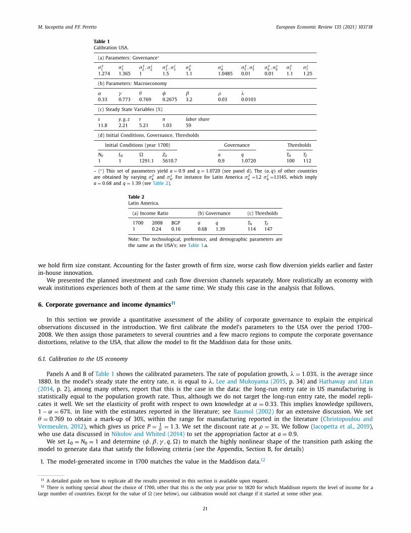
M. Iacopetta and P.F. Peretto European Economic Review 135 (2021) 103718
Table 1 Calibration USA.
(a) Parameters: Governance ∗
σ F 1 σ I
1 σ F 2 , σ I
2 σ F 3 , σ I
3 σ F 4 σ I
4 σ F 5 , σ I
5 σ F 6 , σ I
6 σ F 7 σ I
7 1.274 1.365 1 1.5 1.1 1.0485 0.01 0.01 1.1 1.25
(b) Parameters: Macroeconomy
α γ θ φ β ρ λ0.33 0.773 0.769 0.2675 3.2 0.03 0.0103
(c) Steady State Variables (%)
s y, g, z r n labor share 11.8 2.21 5.21 1.03 59
(d) Initial Conditions, Governance, Thresholds
Initial Conditions (year 1700) Governance Thresholds
N 0 L 0 # Z 0 a q T N T Z 1 1 1291.1 5610.7 0.9 1.0720 100 112
– ( ∗) This set of parameters yield a = 0 . 9 and q = 1 . 0720 (see panel d). The (a, q ) of other countries are obtained by varying σ F
4 and σ I 4 . For instance for Latin America σ F
4 = 1.2 σ I 4 = 1.1145, which imply
a = 0 . 68 and q = 1 . 39 (see Table 2 ).
Table 2 Latin America.
(a) Income Ratio (b) Governance (c) Thresholds
1700 2008 BGP a q T N T Z 1 0.24 0.16 0.68 1.39 114 147
Note: The technological, preference, and demographic parameters are the same as the USA’s; see Table 1 .a.
we hold firm size constant. Accounting for the faster growth of firm size, worse cash flow diversion yields earlier and faster
in-house innovation.
We presented the planned investment and cash flow diversion channels separately. More realistically an economy with
weak institutions experiences both of them at the same time. We study this case in the analysis that follows.
6. Corporate governance and income dynamics 11
In this section we provide a quantitative assessment of the ability of corporate governance to explain the empirical
observations discussed in the introduction. We first calibrate the model’s parameters to the USA over the period 1700–2008. We then assign those parameters to several countries and a few macro regions to compute the corporate governance
distortions, relative to the USA, that allow the model to fit the Maddison data for those units.
6.1. Calibration to the US economy
Panels A and B of Table 1 shows the calibrated parameters. The rate of population growth, λ = 1 . 03% , is the average since
1880. In the model’s steady state the entry rate, n, is equal to λ. Lee and Mukoyama (2015 , p. 34) and Hathaway and Litan
(2014 , p. 2), among many others, report that this is the case in the data: the long-run entry rate in US manufacturing is
statistically equal to the population growth rate. Thus, although we do not target the long-run entry rate, the model repli-
cates it well. We set the elasticity of profit with respect to own knowledge at α = 0 . 33 . This implies knowledge spillovers,
1 − α = 67% , in line with the estimates reported in the literature; see Baumol (2002) for an extensive discussion. We set
θ = 0 . 769 to obtain a mark-up of 30%, within the range for manufacturing reported in the literature ( Christopoulou and
Vermeulen, 2012 ), which gives us price P = 1 θ = 1 . 3 . We set the discount rate at ρ = 3% . We follow ( Iacopetta et al., 2019 ),
who use data discussed in Nikolov and Whited (2014) to set the appropriation factor at a = 0 . 9 .
We set L 0 = N 0 = 1 and determine ( φ, β, γ , q, #) to match the highly nonlinear shape of the transition path asking the
model to generate data that satisfy the following criteria (see the Appendix, Section B, for details)
1. The model-generated income in 1700 matches the value in the Maddison data. 12
11 A detailed guide on how to replicate all the results presented in this section is available upon request. 12 There is nothing special about the choice of 1700, other that this is the only year prior to 1820 for which Maddison reports the level of income for a
large number of countries. Except for the value of # (see below), our calibration would not change if it started at some other year.
21
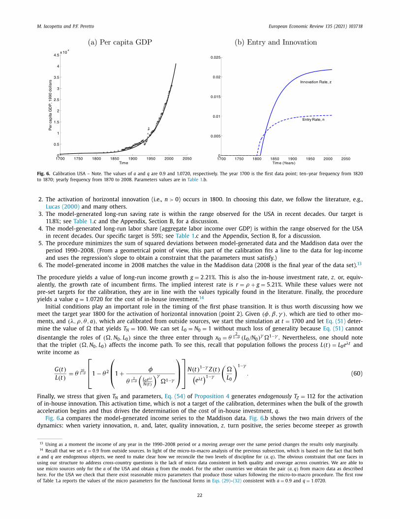
M. Iacopetta and P.F. Peretto European Economic Review 135 (2021) 103718
Fig. 6. Calibration USA – Note. The values of a and q are 0.9 and 1.0720, respectively. The year 1700 is the first data point; ten–year frequency from 1820 to 1870; yearly frequency from 1870 to 2008. Parameters values are in Table 1 .b.
2. The activation of horizontal innovation (i.e., n > 0 ) occurs in 1800. In choosing this date, we follow the literature, e.g.,
Lucas (20 0 0) and many others.
3. The model-generated long-run saving rate is within the range observed for the USA in recent decades. Our target is
11.8%; see Table 1 .c and the Appendix, Section B, for a discussion.
4. The model-generated long-run labor share (aggregate labor income over GDP) is within the range observed for the USA
in recent decades. Our specific target is 59%; see Table 1 .c and the Appendix, Section B, for a discussion.
5. The procedure minimizes the sum of squared deviations between model-generated data and the Maddison data over the
period 1990–2008. (From a geometrical point of view, this part of the calibration fits a line to the data for log-income
and uses the regression’s slope to obtain a constraint that the parameters must satisfy.)
6. The model-generated income in 2008 matches the value in the Maddison data (2008 is the final year of the data set). 13
The procedure yields a value of long-run income growth g = 2 . 21% . This is also the in-house investment rate, z, or, equiv-
alently, the growth rate of incumbent firms. The implied interest rate is r = ρ + g = 5 . 21% . While these values were not
pre-set targets for the calibration, they are in line with the values typically found in the literature. Finally, the procedure
yields a value q = 1 . 0720 for the cost of in-house investment. 14
Initial conditions play an important role in the timing of the first phase transition. It is thus worth discussing how we
meet the target year 1800 for the activation of horizontal innovation (point 2). Given ( φ, β, γ ) , which are tied to other mo-
ments, and ( λ, ρ, θ , a ) , which are calibrated from outside sources, we start the simulation at t = 1700 and let Eq. (51) deter-
mine the value of # that yields T N = 100 . We can set L 0 = N 0 = 1 without much loss of generality because Eq. (51) cannot
disentangle the roles of ( #, N 0 , L 0 ) since the thr ee enter thr ough x 0 = θ2
1 −θ ( L 0 /N 0 ) γ #1 −γ . Nev ertheless, one should note
that the triplet ( #, N 0 , L 0 ) affects the income path. To see this, recall that population follows the process L ( t ) = L 0 e λt and
write income as
G ( t )
L ( t ) = θ
2 θ1 −θ
1 − θ2
1 + φ
θ2
1 −θ
(L 0 e λt N ( t )
)γ
#1 −γ
N ( t )
1 −γ Z ( t ) (e λt
)1 −γ
(#
L 0
)1 −γ
. (60)
Finally, we stress that given T N and parameters, Eq. (54) of Proposition 4 generates endogenously T Z = 112 for the activation
of in-house innovation. This activation time, which is not a target of the calibration, determines when the bulk of the growth
acceleration begins and thus drives the determination of the cost of in-house investment, q .
Fig. 6 .a compares the model-generated income series to the Maddison data. Fig. 6 .b shows the two main drivers of the
dynamics: when variety innovation, n, and, later, quality innovation, z, turn positive, the series become steeper as growth
13 Using as a moment the income of any year in the 1990–2008 period or a moving average over the same period changes the results only marginally. 14 Recall that we set a = 0 . 9 from outside sources. In light of the micro-to-macro analysis of the previous subsection, which is based on the fact that both
a and q are endogenous objects, we need to make clear how we reconcile the two levels of discipline for ( a, q ) . The obvious constraint that one faces in using our structure to address cross-country questions is the lack of micro data consistent in both quality and coverage across countries. We are able to use micro sources only for the a of the USA and obtain q from the model. For the other countries we obtain the pair ( a, q ) from macro data as described here. For the USA we check that there exist reasonable micro parameters that produce those values following the micro-to-macro procedure. The first row of Table 1.a reports the values of the micro parameters for the functional forms in Eqs. (29) –(32) consistent with a = 0 . 9 and q = 1 . 0720 .
22

M. Iacopetta and P.F. Peretto European Economic Review 135 (2021) 103718
accelerates. The model matches quite well the data for the second half of the 20th century. For example, in the years 1950,
1975, 1990, and 2005, the model predicts 97%, 97%, 94%, and 103% of the data. It does less well in the 19th century, however,
underpredicting the data by 10%-20% on average (see Appendix, Table 5).
6.2. Relative income dynamics around the world
To what extent are cross-country income differences are attributable to delays in industrialization caused by corporate
governance distortions? Clearly, channels other than corporate governance contribute to cross-country income difference
and thus, to the extent that we do not account for them explicitly, our estimates of q and a are upper and lower bounds,
respectively, of the actual ones. We use two constraints to discipline our cross-country exercise. First, we use the same set
of parameters for all countries, allowing them to differ only by corporate governance and, possibly, by the factor # of the
final good sector. Second, in determining the pair (a, q ) we use Eq. (57) to construct the corporate governance loci
q ( a ) = αφβρ
( g ∗ + ρ) [(1 − α)
(1 θ − 1
)− βρ
a
]+
(1 θ − 1
)αρ
. (61)
and then impose a common growth rate of income, g ∗, for all countries. The above expression says that q is decreasing in
a . 15 Because, as we discussed in Section 5 , the appropriation factor, a, raises the incentives to enter and thus produces an
equilibrium market structure with a larger mass of smaller firms that invest less. Accordingly, our exercises postulate that
better a is associated to a compensatory change in q that keeps constant the long-run growth rate. Therefore, they identify
and isolate the activation dates T N and T Z as the channels through which corporate governance shapes the path of income.
To fix the ideas on the relationship between income differences, governance, and industrialization thresholds, it is useful
to compare the development patterns of USA and Latin America. According to Maddison data, in the early 18th century per
capita income in the Latin America region was about the same as that in the USA; three centuries later, however, Latin
America has an average income of only a quarter that of the USA. Assuming that neither of the two regions had an initial
advantage on the other, in terms of land, technology, or human capital, that is that they had the same # – arguably a
reasonable assumption in view of their comparable initial income – we estimate a value of the pair ( a, q ) for Latin America
of (0.68,1.39), compared to (0.9,1.07) for the USA. Thus the corporate quality difference between the two regions, expressed
( 0a, 0q ) is ( −0 . 22 , 0 . 32 ), meaning that in Latin America the shareholders appropriation factor and the internal cost of
capital are 22 percent smaller and 32 percent higher than in the USA, respectively. Such difference implies delays in the
activation thresholds of the second and third phases for 0T N = 14 and 0T Z = 35 years, respectively. The model’s out-of-
sample prediction is that the income ratio will decline further along the transition to the steady state, from 0.24 in 2008 to
0.16. Observe that the predicted increase in income gap is explained exclusively by the difference in corporate governance
distortions because we are using the same set of parameters, reported in Table 1 .b, and the same value of # for the two
economies. The main insight of this exercise, that also characterize the more general cross-country results to be discussed
below, is that frictions and delays that are seemingly relatively small can produce large income differences over time because
they drive long-lasting differences in growth rates.
6.2.1. Cross-Country analysis
According to Maddison data in 1700 relative to the USA per capita income was higher in Western Europe and somewhat
lower in a few Asian and several African countries. We account for such initial differences through the exogenous produc-
tivity factor #. This initial income gaps that could be due to differences in technology, human capital, or natural resources –fertility of land, the availability of fresh water, navigable rivers, access to seaports. Everything else equal, an economy with
relatively large # reaches the first activation threshold, x N , relatively early. The higher the initial income, the smaller the
expansion between 170 0 and 20 08 to be accounted for by the model and the worse (lower a, higher q ) is the corporate
governance. Thus, # has two opposite effects on the take-off time: it reduces T N by increasing the initial condition x 0 ; it
raises T N by generating a lower appropriation factor, a . To decompose the two effects, we first calculate ( a, q ) and ( T N , T Z )
with the income ratio observed in the data and then recalculate ( T N , T Z ) under the same pair ( a, q ) but using the # of the
USA.
UK, Western Europe and the USA. Fig. 7 visualizes the take-off of the UK and that of the USA: The relatively higher initial
income in the UK implies that industry variety expands there at an earlier time. The subsequent takeover of the USA is
due to the better corporate governance: While the UK’s larger # moves the take-off earlier in time by 39 years, the worse
corporate governance raises T N and T Z by 14 and 35 years, respectively. The net effect is that the UK and the USA enter
the third phase at about the same time but the USA grows faster and eventually pulls ahead. Table 3 .b summarizes similar
estimates for 12 European countries. Relative to the USA, these countries have on average a smaller appropriation factor
( 0a = −0 . 19 ) and greater cost of capital ( 0q = 0 . 25 ); the differences in take-off times for the second and third phases are
0T N = −17 , and 0T Z = −1 , meaning that Western Europe starts, on average, the two transition phases earlier than the USA
by seventeen years and one year, respectively. According the our estimates, however, its initial advantage (larger #) plays a
15 Fig. 2 in the Appendix illustrates the quantitative relation that we obtain with our calibrated parameters for a range of values of g ∗ . The figure suggests that allowing long-run growth to differ across countries would not change the results by much unless such differences are very large.
23

M. Iacopetta and P.F. Peretto European Economic Review 135 (2021) 103718
Fig. 7. USA takes over UK – Note. The values of (a, q ) are (0.9, 1.0702) and (0.7, 1.3420) for USA and UK, respectively. For common parameters values see Table 1 .b.
Table 3 Industrialization Delays: Western Europe.
(a) p.c. GDP (b) Governance and delays
Year a q 0T N 0T Z
Country 1700 1820 2008 C. G. I. C. Total C. G. I. C. Total
Austria 1.88 0.97 0.77 0.71 1.32 11 26 15 27 26 1 Belgium 2.17 1.05 0.76 0.69 1.36 13 34 21 32 34 2 Denmark 1.97 1.01 0.79 0.72 1.30 10 28 18 25 29 4 Finland 1.21 0.62 0.78 0.79 1.19 6 7 1 13 7 6 France 1.73 0.90 0.71 0.73 1.28 10 22 12 23 22 1 Germany 1.72 0.86 0.67 0.72 1.30 10 21 11 25 22 3 Italy 2.08 0.89 0.64 0.69 1.36 13 32 19 32 31 1 Netherlands 4.04 1.46 0.79 0.61 1.61 20 73 53 62 73 11 Norway 1.37 0.64 0.91 0.80 1.17 5 11 6 11 11 0 Sweden 1.42 0.65 0.78 0.77 1.22 7 13 6 16 14 2 Switzerland 1.69 0.87 0.80 0.75 1.25 8 20 12 19 21 2 UK 2.37 1.36 0.76 0.68 1.39 14 39 25 35 39 4 W. Europe (12) 1.95 0.98 0.71 0.71 1.32 11 28 17 27 28 1
Note: The technological, preference, and demographic parameters are the same as the USA’s; see Table 1 .b. 0 indicates a country’s or region’s difference with respect to the USA estimated values.
major role in explaining European countries’s faster crossing of the two critical transition thresholds – industry variety and
in-house investment. Once such initial advantage is controlled for, it is the USA that, thanks its better quality of corporate
governance, crosses the two thresholds sooner: by eleven years that of industry variety and by twenty-seven years that of
in-house investment.
6.3. Model vs. data
Technological progress has been an unrelenting force fueling income expansion over the last three centuries. Yet, political
upheavals, revolutions, civil wars, global conflicts and other events, like plagues and natural disasters, disturbed the smooth
transition to modern growth. The model abstracts from these factors. It is thus instructive to check how the model fares
with respect to the cross-sectional evidence summarized in Fig. 1 , which shows that the quality of governance is negatively
associated with the waiting time for the first growth acceleration, and with respect to time-series evidence on income per
capita. Fig. 8 .a documents a strong positive correlation (0.72) between our estimates of the appropriation factor, a, and the
World Bank governance index for the year 2017 (the quality of contract enforcement and the strength of property rights are
two key components of the index, see Kaufmann et al. 2010). 16 Similarly, Fig. 8 .b documents a strong negative correlation
16 While the governance index is available as far a back as 1996, it is has a more limited coverage. For instance, for the year 1996 no data is provided for Argentina, Australia, and Switzerland, among others.
24

M. Iacopetta and P.F. Peretto European Economic Review 135 (2021) 103718
Fig. 8. Model vs. Data – Note. For list of countries see note of Fig. 1 . The digits inside the plots C and D indicate the number of countries. Countries that do not reach the third phase ( z = 0 ) are excluded from the calculation. These are: Haiti and Nepal (period 3); Madagascar, Liberia, Somalia, and Angola (period 4); Rep. Dem. of Congo, Burundi, Comoros, Togo, Guinea-Bissau, Guinea, Sierra Leone, Malawi, Tanzania, Zambia, Eritrea, Mongolia, Rwanda, Gambia, Burkina Faso, Kenia, Mali, and Laos (period 5); Bangladesh (period 6); Chad, Afhanistan, Uganda, and Sudan (period 7).
( −0 . 64 ) between the World Bank governance index and our estimates of the cost of investment, q . This pattern suggests
that the model is on the right track with respect to the motivational evidence provided in Fig. 1 .
Fig. 1 also indicate there are large differences in take-off times across groups of countries. Propositions 3 and 4 state that
countries with worse corporate governance cross the variety-expansion and quality-innovation thresholds with some delay.
Panels C and D of Fig. 8 report the average delays in crossing the thresholds x Z and x N relative to the USA for each group of
countries by period of take-off reported in Fig. 1 . The objective is to compare the model to the data in this key dimension
of our exercise. We focus on the delay measured by T Z as this characterizes the transition to the innovation economy. Of the
155 countries of Fig. 1 , we leave out a few countries for which the model predicts T Z → ∞ , i.e., they converge to the steady
state with z = 0 . 17 For countries that take off in period 2 (between 1820 and 1870), the model predicts an average delay of
about 17 years. For countries that take off in period 3 (1870–1900), the predicted average delay is approximately 52 years.
Since the model predicts that in the USA quality-innovation starts in 1812 (see Table 1 ), the average delays of 17 and 53
years imply the years 1829 and 1865, respectively, as the take-off times for the countries that take off in periods 2 and 3.
Hence for the period 3 the model’s prediction is 5 years short of the beginning of the time interval 1870–1900.
With the exception of Italy, by the turn of the century all major Western economies have experienced the first growth
acceleration. The period 1900–1950 covers the two world wars and the great depression. Our model predicts, on average, a
60 years lag for the group of countries that took off in this period and thus underpredicts their delay by about 30 years.
Similarly it underpredicts the delay of the group of countries that took off in the post-war period 1950–1975. The Appendix,
Section C, elaborates further on the cross-country prediction of the model, by comparing the per capita income path calcu-
lated according to the estimated pair ( a, q ) and initial factor # of each country or macro-region and Maddison income time
17 The note of Fig. 8 provides a complete list of the excluded countries.
25

M. Iacopetta and P.F. Peretto European Economic Review 135 (2021) 103718
Fig. 9. Governance Shock in 1950 – Note. Continuous lines: constant governance. Dashed lines: in 1950 a increases by 0.1 and q adjusts to preserve the growth rate. The fit of the model improves in Japan but worsens in UK (see Appendix, Section C, for details). For parameters values see Table 1 .b. Data time series are per capita GDP, 1990 dollars.
series. Next, we comment on well-known Asian economic miracles and whether postulating a level-change in the quality of
governance accounts for the longer-than-predicted wait time to take-off.
6.4. Where the model fails: Improved corporate governance?
In the post-WWII period several countries experienced transformations that arguably affected corporate governance. For
instance, the USA imposed the dismantling of the ziabatsu system in Japan. As a result, several family-dominated companies
were dissolved and interlocking directorships were outlawed. Such a radical reform increased accountability and reduced
agency frictions. To explore this hypothesis, we allow for a shock that improves corporate governance in 1950. Specifically,
we introduce unanticipated and permanent changes to the parameters of the equations describing the costs of resource
diversion that result in an increase of a by 0.1 and a decrease of q by 0.1. Because we implement this change under the
constraint that both the growth rate and the level of income at the end of the simulation remain the same, we are asking
the model to produce a longer period of stagnation, because of bad corporate governance before 1950, and a more drastic
acceleration of growth after 1950 due to the improvement in corporate governance. Fig. 9 .a shows the main result: allowing
post-war Japan to experience better corporate governance improves the fit, narrowing the gap between model and data by
more than 10 percentage points. The same conclusion applies to other fast-growing Asian countries such as China, South
Korea and Singapore: a post-war shock to governance improves the fit of model. In contrast, in the case Western Europe
as a macro region, the USA, UK, Germany, or France, as well as in Latin America a similar positive governance shock would
worsen the model’s performance. Interestingly, we find some support for the hypothesis that improvements in corporate
governance occurred in some northern European countries, most notably, Sweden, Norway, Finland, and in the Netherlands
and Italy. 18
That a post-war governance shock is more likely to apply to Asian than Latin American countries is in line with the
historical observation that WWII was not a disruptive event for Latin America, surely not disruptive on a scale comparable to
what occurred in Asia. And the conclusion that the dynamics of income of our macro regions and of leading economies like
the USA, UK and Germany, does not require changes in fundamentals is also in agreement with arguments that attribute the
contemporary income gaps of Latin American countries to the extractive-type of institutions that emerged in colonial times
( Engerman and Sokoloff, 1997; Acemoglu and Robinson, 2012 ) and with the observation that modern economic institutions,
including the basic elements of the modern corporation, developed in Europe centuries priors the onset of modern growth
( Goetzmann, 2016 , chapter 17; Le Bris et al., 2016 ).
More generally, our analysis provides some support to Fukuyama’s interpretation (2014, chapter 23) of Asian rapid indus-
trialization, namely, that the executive power of the government substituted for the lack of the rule of law that in Western
countries provided the foundation for modern corporate governance. The confrontation with Western colonial powers dis-
rupted then state institutions that were formed centuries prior to contact with the West.
18 See the Appendix, Section C, for details.
26

M. Iacopetta and P.F. Peretto European Economic Review 135 (2021) 103718
7. Conclusion
Several recent studies emphasize the importance of corporate governance in explaining cross-country income differences.
In this paper, we developed the long-run features and implications of this view by introducing in an innovation-led growth
model within-firm principal-agent problems among shareholders, managers and directors (monitors). The model features a
sequence of three phases, from a pre-industrial phase, through a takeoff phase, to the modern innovation economy phase.
Our analysis shows that the severity of agency issues delays the economy’s progress through the three phases. This result is
in line with Fig. 1 , which documents a negative relation between the first growth acceleration and the rule of law score for
a sample of 155 countries. Our analysis also shows that poor corporate governance can be a forbidding barrier that traps
the economy in stagnation. Finally, conditional on takeoff, poor corporate governance weakens incentives to innovate and
thus slows down the secular growth of productivity.
To assess how well corporate governance explains quantitatively the secular dynamics of relative incomes, we calibrated
the model to the USA and conducted exercises that compare the income paths of economies that converge to a common
growth rate but diverge in levels, allowing only corporate governance to differ across economies. We found that modest
differences in corporate governance produce large differences in income. We calculated, for instance, that the cost of in-
house investment in Latin America, which in 2008 had income a quarter of that of the USA and is predicted to decline to
16 percent in steady state, is only 32% more than in the USA. This divergence, moreover, depends on a delay in the first
onset of industrialization, driven by entry of new firms with no in-house investment by incumbent firms yet, of only 14
years and a further delay in the onset of in-house innovation of 35 years. This finding is in contrast with previous studies
that need much larger differences in the cost of capital to account for the observed income divergence over the transition to
modern growth. The shape of the transition generated by the model drives our different estimate for the cost of investment.
Specifically, in our framework the rates of entry and of in-house innovation pick up slowly. Consequently, a small delay in
the onset of modern growth has large compounding effects on the income gap from early movers.
We have also conducted exercises to verify how well the agrees with the pattern produced by different metrics like the
World Bank rule of law score, the take-off periods, and the income paths of individual countries. The model’s endogenous
variables that represent agency issues, a and q, are strongly correlated with the rule of law indicator. The model also fits
the income data remarkably well. Our estimates of delayed industrialization are also highly correlated with the accelera-
tion times observed in the data. The model, nevertheless, tends to underestimate the take-off time of countries that have
experienced economic miracles in the post-WWII period.
We kept the institutional environment constant to isolate the role corporate governance and see how far it takes us
without invoking changes in other fundamentals. We then allowed for a change in the model’s micro parameters that results
in better corporate governance in the post-WWII period. The level-change improves the model’s fit of the data only for Asian
countries and it actually worsens it for Western countries. This pattern is consistent with the idea that while in the West
the fundamental features of the institutional environment developed prior to industrialization and remained largely stable,
in other areas they changed drastically in the aftermath of WWII.
Supplementary material
Supplementary material associated with this article can be found, in the online version, at 10.1016/j.euroecorev.2021.
103718 .
References
Acemoglu, D. , Robinson, J.A. , 2012. Why Nations Fail: the Origins of Power, Prosperity and Poverty. Crown, New York . Aghion, P. , Howitt, P. , Mayer-Foulkes, D. , 2005. The effect of financial development on convergence: theory and evidence. Q. J. Econ. 120, 173–222 . Aghion, P. , Reenen, J.V. , Zingales, L. , 2013. Innovation and institutional ownership. Am. Econ. Rev. 13, 277–304 . Balsmeier, B. , Fleming, L. , Manso, G. , 2016. Independent boards and innovation. J. Financ. Econ. 123 (3), 536–557 . Baumol, W.J. , 2002. The Free-Market Innovation Machine: Analyzing the Growth Miracle of Capitalism. Princeton University Press, Princeton, NJ. . Celik, M., Tian, X., 2019. Agency frictions, managerial compensation, and disruptive innovation. Available at SSRN: https://ssrn.com/abstract=3319148 . Christopoulou, R. , Vermeulen, P. , 2012. Markups in the euro area and the US over the period 1981–2004: a comparison of 50 sectors. Empir. Econ. 42 (1),
53–77 . Chu, A.C. , Cozzi, G. , Galli, S. , 2014. Stage-dependent intellectual property rights. J. Dev. Econ. 116, 239–249 . Chu, A.C. , Kou, Z. , Wang, X. , 2019. Effects of patents on the transition from stagnation to growth. J. Popul. Econ. . Forthcoming Cooley, T.F. , Quadrini, V. , 2001. Financial markets and firm dynamics. Am. Econ. Rev. 5, 1286–1310 . Doidge, C. , Karolyi, G.A. , Stulz, R.M. , 2007. Why do countries matter so much for corporate governance? J. Financ. Econ. 86, 1–39 . Engerman, S.L. , Sokoloff, K.L. , 1997. Factor endowments, institutions, and differential paths of growth among new world economies. In: Haber, S. (Ed.), How
Latin America Fell Behind. Stanford University Press, Stanford, CA 1997 . Fukuyama, F. , 2014. Political order and political decay: From the industrial revolution to the globalization of democracy. London Profile Books . Fulghieri, P. , Suominen, M. , 2012. Corporate governance, finance, and the real sector. J. Financ. Quant. Anal. 47, 1187–1214 . Goetzmann, W.N. , 2016. Money Changes Everything: How Finance Made Civilization Possible. Princeton University Press . Greif, A. , 2006. Institutions and the Path to the Modern Economy: Lessons from Medieval Trade. Cambridge University Press . Hathaway, I. , Litan, R.E. , 2014. What’s driving the decline in the firm formation rate? A Partial Explanation, Economic Studies, at Brookings . Hausmann, R. , Pritchett, L. , Rodrik, D. , 2005. Growth accelerations. J. Econ. Growth 10 (4), 303–329 . Iacopetta, M. , Minetti, R. , Peretto, P. , 2019. Financial markets, industry dynamics, and growth. Econ. J. . Forthcoming Kaufmann, D. , Kraay, A. , Mastruzzi, M. , 2010. The Worldwide Governance Indicators: a Summary of Methodology, Data and Analytical Issues. World Bank
Policy Research Working Paper No. 5430 .
27

M. Iacopetta and P.F. Peretto European Economic Review 135 (2021) 103718
Le Bris, D., Goetzmann, W. N., Pouget, S., 2016. Testing asset pricing theory on six hundred years of stock returns: prices and dividends for the bazacle company from 1372 to 1946. Manuscript.
Lee, Y. , Mukoyama, T. , 2015. Entry and exit of manufacturing plants over the business cycle. Eur. Econ. Rev. 77, 20–27 . Lins, K.V. , Servaes, H. , Tamayo, A. , 2017. Social capital, trust, and firm performance: the value of corporate social responsibility during the financial crisis. J.
Financ. 72 (4), 1785–1824 . Lopez, A.L. , Vives, X. , 2019. Overlapping ownership, r&d spillovers, and antitrust policy. J. Polit. Econ. 127 (5), 2394–2437 . Lucas, R.E. , 20 0 0. Some macroeconomics for the 21st century. J. Econ. Perspect. 14, 159–168 . Maddison Database, 2010. Available at https://www.rug.nl/ggdc/historicaldevelopment/maddison/releases/maddison- database- 2010 . Accessed on 23/10/2017. Madsen, J. B., Minniti, A., Venturini, F., 2019. Wealth inequality in the long run: a schumpeterian growth perspective. Manuscript. Morck, R. , Wolfenzon, D. , Yeung, B. , 2005. Corporate governance, economic entrenchment, and growth. J. Econ. Lit. 43, 655–720 . Nikolov, B. , Whited, T. , 2014. Agency conflicts and cash: estimates from a dynamic model. J. Financ. 69, 1883–1921 . Peretto, P.F. , 2015. From smith to schumpeter: a theory of take-off and convergence to sustained growth. Eur. Econ. Rev. 78, 1–26 . Shleifer, A. , Wolfenzon, D. , 2002. Investor protection and equity markets. J. Financ. Econ. 66 (1), 3–27 . Terry, J. S., 2017. The macro impact of short-termism. Available at http://people.bu.edu/stephent/files/MIFET _ LATEST _ DRAFT.pdf . Accessed 12/02/2019.
28