ET 438B Sequential Control and Data Acquisition … · Sequential Control and Data Acquisition Laboratory 7 PLC Function Programming Using Ladder Logic ... Write Boolean state equations

Spring 2015 1 Lab7_ET438b.docx

ET 438B

Sequential Control and Data Acquisition

Laboratory 7

PLC Function Programming Using Ladder Logic

Laboratory Learning Objectives

1.) Explain the operation of on and off delay timers used in ladder logic and use them in

programming exercises

2.) Explain the operation of up/down counters used in ladder logic programs and use them in

programming exercises.

3.) Define operating states of a given physical system

4.) Write Boolean state equations for a physical system and use them to program ladder logic.

Technical Background

Programmable Logic Controllers have other uses along with the implementation of ladder logic

in software. Two of the most common functions are those of timing processes and counting

events. These functions replace the costly electromechanical and discrete electronic devices

used to accomplish the tasks before the arrival of PLCs. Time driven processes we see in the

home are automatic washing machines and clothes dryers. A timing device controls a sequence

of events in these processes moving the appliances from one operating state to another. Boolean

state equations provide an mathematical basis for describing time and event driven processes.

Designs based on well thought out Boolean state equations produce control programs that are

less likely to have logical errors and have clearer structures.

Timer Functions

On-delay and off-delay timers provide fundamental timing functions in sequential control

systems. Figure 1 shows the schematic symbols for electromechanical timer relays and contacts.

Timer coils can have either two or three-wire representations and usually have labels that

indicate the device is a timer (e.g. TR). Contacts associated with the coil have the same

identifier with a sequence number that indicate the linkage between the coil and the contacts

(e.g. the coil TR controls TR1, TR2, TR3). Figure 1 also shows the contact symbols associated

both the on and off delay devices.

On-delay timers must have their coils' energized before the timing sequence can start. All

contacts associated with the coils change state after a predetermined time interval. Off-delay

timers maintain contact states when their coils' are energized but start the timing period AFTER

the coil is de-energized. All associate contacts will change states after the timers preset interval


when the coil is de-energized. Electromechanical/Electronic timers were expensive. PLCs

implement both timing functions in electronic hardware and software at a fraction of the cost.

Off-delay

Normally

Open

Off-delay

Normally

Closed

On-delay

Normally

Closed

On-delay

Normally

OpenTR

TR

Coils

Figure 1. Electromechanical Timer Schematic Symbols.

The Micro800 series PLCs have both on-delay and off-delay functions accessible from the Block

menu choice in the ladder diagram programming palette of the toolbox in Connected

Components Workbench. Figure 2 shows the ladder diagram symbols for both the on and off

delay timers. The TON block provides the on-delay timing function while the TOF implements

Figure 2. TOF and TON Timer Functions in the Connected Components Workbench

Development Environment.

the off-delay timer. Timers must be the output of a rung. The Boolean result of the rung

conditions and the timer type determine the action of the outputs. An off-delay timer begins its

timing sequence when the timer input transitions from TRUE to FALSE. If the input rung

condition changes from FALSE to TRUE before the preset time delay ends, then the timer resets.


Table 1 shows the parameters of the TOF function. The parameter IN takes the Boolean result of

the rung evaluation into the timer. A TRUE to FALSE transition on this input starts the timer.

The time diagram in Figure 3 shows how the TOF function's I/O signals interact.

Table-1 TOF-Off-Delay Timer Function Parameters

Parameter Parameter Type Data Type Description

IN Input Boolean T to F starts timer

F to T stops and resets timer

PT Input Time Programmed Time delay

Format t#HHhMMmSSsMMms where HH is

number of hours, MM is minutes, SS is

seconds and MM is miliseconds.

Q Output Boolean Timer output. Stays TRUE while timer

elapsed time value is less than PT value.

Becomes FALSE when ET=PT.

ET Output Time Displays current value of elapsed time when

CCW is in debug mode.

Parameter Range: 0ms - 1193h2m47s294ms

IN

0

PT

Q

ET ET<PT

Figure 3. TOF Timing Diagram Showing the Sequence of Operation.

Note that the output, Q remains high only while the timer function internal timer is less that the

preset value defined by PT.


The on-delay timer function TON is the logical opposite of the TOF function. Table 2 describes

the actions of the function's parameters. This function delays its TRUE output until after the

timer value reaches the preset value. Figure 4 shows the timing diagram for the TON function.

The TON function resets when the input parameter, IN, becomes FALSE before ET=PT

Table-2 TON-On-Delay Timer Function Parameters


IN Input Boolean F to T starts timer

T to F stops and resets timer

PT Input Time Programmed Time delay

Format t#HHhMMmSSsMMms where HH is

number of hours, MM is minutes, SS is

seconds and MM is miliseconds.

Q Output Boolean Timer output. Stays FALE while timer elapsed

time value is less than PT value. Becomes

TRUE when ET=PT.

ET Output Time Displays current value of elapsed time when

CCW is in debug mode.

Parameter Range: 0ms - 1193h2m47s294ms

.

IN

0

PT

Q

ET ET<PT

Figure 4. TON Function Timing Diagram Showing Timer Reset.


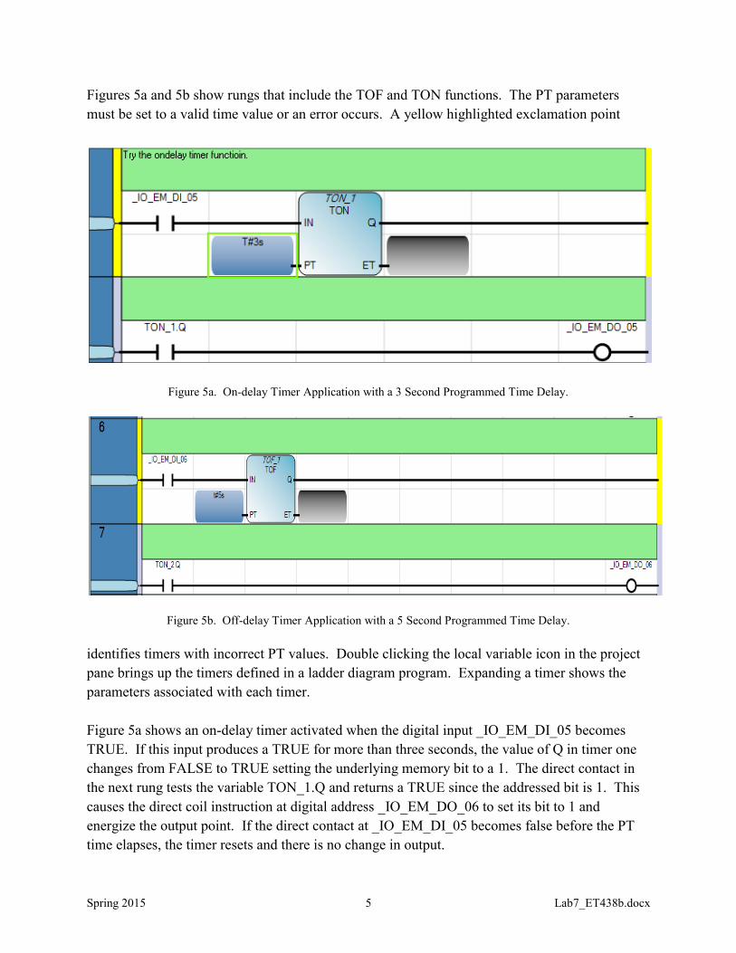
Figures 5a and 5b show rungs that include the TOF and TON functions. The PT parameters

must be set to a valid time value or an error occurs. A yellow highlighted exclamation point

Figure 5a. On-delay Timer Application with a 3 Second Programmed Time Delay.

Figure 5b. Off-delay Timer Application with a 5 Second Programmed Time Delay.

identifies timers with incorrect PT values. Double clicking the local variable icon in the project

pane brings up the timers defined in a ladder diagram program. Expanding a timer shows the

parameters associated with each timer.

Figure 5a shows an on-delay timer activated when the digital input _IO_EM_DI_05 becomes

TRUE. If this input produces a TRUE for more than three seconds, the value of Q in timer one

changes from FALSE to TRUE setting the underlying memory bit to a 1. The direct contact in

the next rung tests the variable TON_1.Q and returns a TRUE since the addressed bit is 1. This

causes the direct coil instruction at digital address _IO_EM_DO_06 to set its bit to 1 and

energize the output point. If the direct contact at _IO_EM_DI_05 becomes false before the PT

time elapses, the timer resets and there is no change in output.


Figure 5b shows the operation of an off-delay timer. This timer has a programmed time delay of

5 seconds. The TOF function actives when the input at address _IO_EM_DI_06 becomes

FALSE. The TOF function starts timing and sets the output parameter TOF_1.Q to TRUE. This

output remains TRUE until the value of ET=PT. If the input point at address _IO_EM_DI_06

changes from FALSE to TRUE before the elapsed time equals programmed time the output

resets to FALSE. The direct contact instruction in the next rung shown in Figure 5b tests the

output variable of the TOF function. When TOF_1.Q=TRUE its memory bit is set to 1, so the

direct contact instruction returns a TRUE and the output addressed by the direct coil instruction

is energized.

The CCW programming environment includes several other timing functions. The Mirco800

Programmable Controllers General Instruction Manual (Rockwell Automation document number

2080-rm001_-en-e.pdf) describes these instructions. Download this reference from the learning

management system or the course website for future use.

Counter Functions

Another common task implemented using a PLC system is to record the number of events that

occur in a sequential system. The counter functions of the PLC replace electromechanical

counters in modern industrial control processes. The Micro800 series of PLCs have three

counter functions: a count-down structure (CTD), a count-up structure (CTU), and a up-down

structure (CTUD). These functions handle a variety of tasks found in sequential control design.

Figure 6 shows the function blocks of the up, down and up/down counters used for ladder

diagram programming. These functions are available from the Block menu choice in the ladder

diagram programming palette of the toolbox in Connected Components Workbench. These are

output functions and should be located on the right side of a ladder diagram rung.

Figure 6. Counter Functions In The Mirco800 PLC .


Tables 3 through 5 list the functional parameters of each structure. Table 3 shows the functional

parameters of the CTD instruction. The CTD has three input parameters. The CD input

decrements the programmed value of the counter by 1 each time the rung input

Table-3 CTD- Count-Down Counter Function Parameters


CD Input Boolean Decreases CV value by 1 when rung make a

FALSE-to-TRUE transition

LOAD Input Boolean Set CV=PV when TRUE

Q Output Boolean Underflow flag: TRUE when CV≤0

PV Input D-Integer Programmed counter value

CV Output D-Integer Current counter value

transitions from FALSE to TRUE. The LOAD input is a Boolean parameter that sets the current

counter value parameter, CV equal to the programmed value, PV when it is TRUE. This can be

used to change the state of the output parameter, Q, before the programmed number of counts

occurs and to reset the counter value to its PV value after the programmed count number occurs.

The function’s outputs are CV, the current count value and Q. The parameter Q indicates when

CTD has registered the programmed number of counts. If becomes TRUE when the current

value parameter, CV reaches 0.

Table 4 lists and defines the CTU function. This counter function increments a value variable

until it reaches a predefined value. The PV parameter sets the maximum number of counts the

Table-4 CTU- Count-Up Counter Function Parameters


CU Input Boolean Increases CV value by 1 when rung make a


RESET Input Boolean Set CV=0 when TRUE

Q Output Boolean Overflow flag: TRUE when CV≥PV

PV Input D-Integer Programmed maximum value


function registers before it gives a TRUE output. The PV and CV data types are double

precision signed integers with a range of ±2,147,483,648 counts. The RESET parameter sets

CV=0 when it is TRUE. This is similar to the LOAD parameter in the CTD function. It can be

used to reset the counter after the programmed number of counts occurs The CTU output

becomes TRUE after the CV value reaches the programmed value, PV.


Table 5 lists the parameters for the CTUD, the up/down counter function. This structure

combines the functions of the up and down counters into a single package. This function has

Table 5 CTUD- Count-Up/Down Counter Function Parameters


CU Input Boolean Increases CV value by 1 when rung make a


CD Input Boolean Decreases CV value by 1 when rung make a


RESET Input Boolean Set CV=0 when TRUE

LOAD Input Boolean Set CV=PV when TRUE

QU Output Boolean Overflow flag: TRUE when CV≥PV

QD Output Boolean Underflow flag: TRUE when CV≤0

PV Input D-Integer Programmed maximum value


two counter inputs, one that increments and another that decrements the current counter value.

There are also two outputs to indicate if the counter has reached 0 or the programmed upper

limit. The RESET and LOAD inputs have the same function in this structure as they have in the

CTU and CTD instructions described previously.

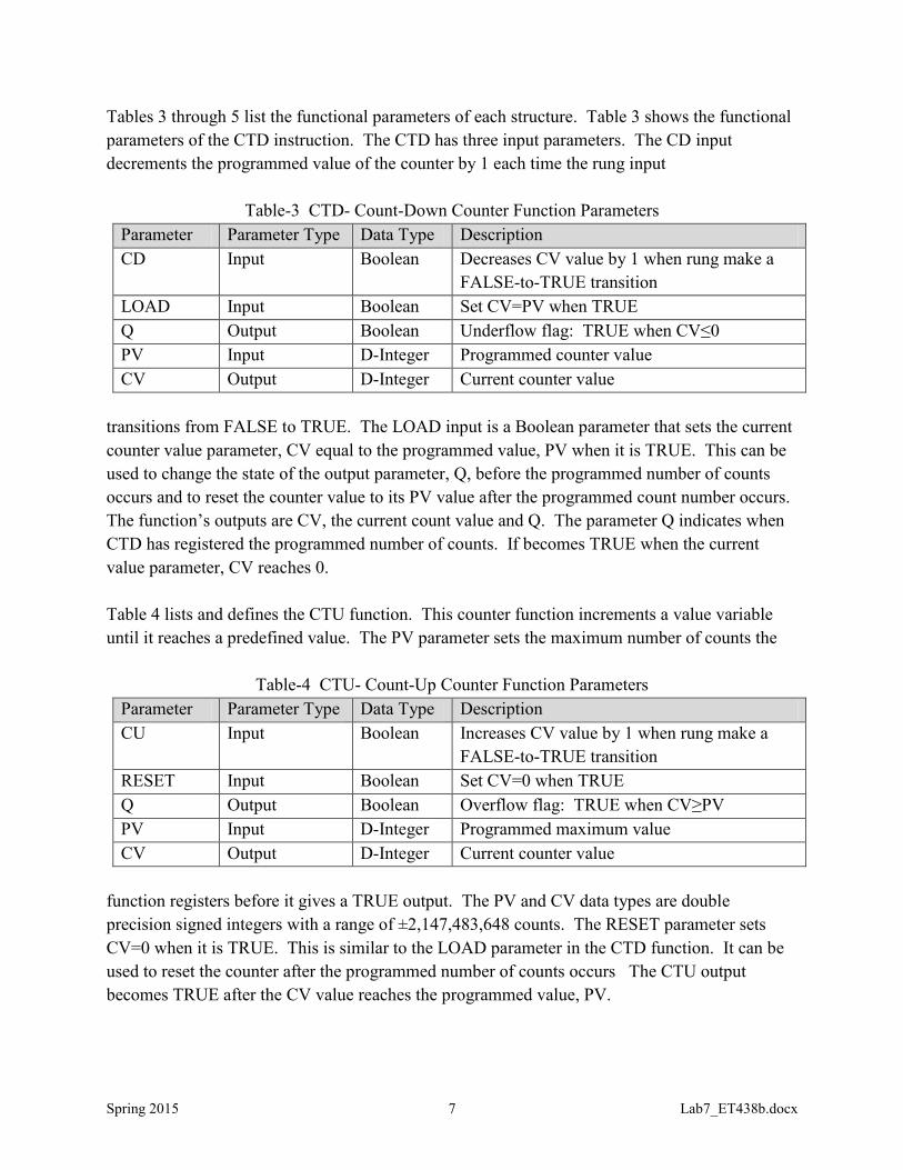
Figures 7 shows the counter functions applied in rungs of ladder logic programming. The CTD

Figure 7. Up and Down Counters in Ladder Logic.


instruction in rung 9 decrements the CV value each time the digital input _IO_EM_DI_11 makes

a FALSE-to-TRUE transition. The value of CV will increase with each transition. The

programmed value is 100, so the value of CTU_1.Q will remain FALSE until the CD input see

100 transitions and the value of CV=0. The LOAD parameter addresses the counter output

value. When the value of CTU_1.Q changes from FALSE to TRUE the LOAD parameter

changes to TRUE and reloads the CV parameter with 100 and the counter can begin

decrementing again from the PV value.

The direct contact in rung 10 links to the CTD function in rung 9. The direct contact addresses

the Boolean output of the CTD function with the CTD_1.Q variable. Each time the CTD counter

function records 100 events the direct contact in rung 10 makes a FALSE-TRUE transition

incrementing the parameter CTU_1.CV. The output of this counter will remain FALSE until

input _IO_EM_DI_11 senses 500 events because the CTU function must increment 5 times

before its output changes. Other program rungs can use CTU_1.Q to trigger events when it

becomes true. The value of CTU_1.CV is reset by an external input, _IO_EM_DI_06.

Mirco800 Programmable Controllers General Instruction Manual gives examples of the use of

the CTUD function. Refer to this document for its use.

Boolean State Equations and Sequential System Design

Inspection and experience can provide solutions to simple sequential control problems but more

complex system require structured methods. Boolean state equations coupled with Boolean

algebra and state diagrams form a set of analytic tools for tackling complex sequential control

problems. The solutions found from using these methods are structured and produce PLC code

that is easily followed and less likely to have logical errors. A state-based design may not

produce a minimal logic design if there are redundant states or the resulting Boolean equations

are not reduced to minimal expressions.

A Boolean state equation provides a formal way of expressing the conditions that cause a

sequential system to enter and leave a given state. An informal statement of a state equation is

State X = (Is currently in state X + Just arrived from another state)∙(has not left to another state)

This expression states that a system is in state X if it was already in state X or logical conditions

cause it to enter state X at this time. The ANDed statements specify logical conditions that would

cause the system to leave the current state.


A formal mathematical version of the state equation gives more specific definitions to the

statement above. Equation (1) shows the formal statement of a state equation. Figure 8 is a

graphic interpretation of the equation.

m

1k

iik

n

1j

jjiii )S)out(T(S)in(TSS (1)

Where S+

i = the next value of the state variable that describes state i

Si = the current value of the state variable i

T(in)ji = logical conditions that would cause process to enter state i from state j

T(out)ik = logical conditions that would cause the process to leave state i

for state k

State variables can take a Boolean value of 1 or 0 to indicate a sequential process is in a given

state.

Si

Sn

S1

S0

Sj

T 0i

T1i

Tji

Tm

i

.

.

.

.

.

.

S+1

m

S+1

1

S+1

0

S+1

k

.

.

.

.

.

.

Ti1

Ti2

Tik

T im

Si

Previous

States

Next

States

Figure 8. Graphical Representation of State Equation Showing Transitions into and out of Si.


The transition equations T(in)ji represent the conditions necessary to set the state variable while

the T(out)ik equations are the conditions necessary to reset the state variable. A state transition

that depends solely on inputs is memoryless. This indicates that the transition is event driven

and does not require information from a previous state. Equation 2 gives the form of a

memoryless state equation. This form indicates neither set or reset functions are state dependent

m

1k

ik

n

1j

jii

1

i ))out(T()in(TSS (2)

The output function relates the process states to the desired output actions. The simplest form of

the output function equates the state variable to the desired output action as shown in equation

(3).

ii OS (3)

Developing a state diagram should be the first step in designing sequential systems that have any

complexity. The most critical step in developing a state diagram is identifying the states. A

designer should consider the system functionality. This includes the following:

1.) normal operating state

2.) internal system behavior changes

3.) external system behavior changes

4.) system sequence of events

After determining a sequence of events, list the modes of operation where the system is

performing one identifiable activity that must be started or stopped. It is possible that waiting for

input is an activity, so the idle state is valid. The designer should also determine what outputs, if

any, entering or leaving a state requires.

Example

A mixing process requires automation in an industrial plant. The process begins when an

operator depresses a momentary contact start push button switch. When the process starts a

solenoid-controlled inlet valve opens and allows a mixture to fill a tank to a specified level. A

float-switch senses when the mixture reaches the correct level. The mixture must be agitated for

20 minutes and then a solenoid controlled outlet valve opens draining the contents into a holding

tank for further processing. The same float switch that detects a full tank senses the tank is

empty. After the tank drains, the system should be ready for another manual start. For safety

reasons, the stop push button should end the process at any point in the sequence. The system

should power up in the stop condition. For this process: a.) define the inputs, the outputs, and the


states, b.) draw a state diagram, c.) write state equations that describe the system operation, d.)

develop a PLC program that performs this control function.

Solution

a.) First define a nomenclature to use in the state diagram.

Sx = process state x , where x is 0, 1,2, 3, … n

Ix = process input x

Ox = process output x

TON(A,T) = on-delay timer function with input A and time setting T in seconds

TOF(A,T) = off-delay timer function with input A and time setting T in seconds

Now define the inputs and outputs from the process description.

Inputs: I0 = first PLC scan

I1= start push button

I2= stop push button

I3=float switch

Outputs: O0=inlet solenoid valve

O1=outlet solenoid valve

O2=agitator motor contactor

Define states for the process. Note that states are not unique. Two different designers may

define the states differently but produce workable designs. The goal should be to describe

system operation using a minimum number of states. Remember, each state will require a

Boolean state equation.

States: S0=stop

S1=start

S2=tank filling

S3= mixture agitating

S4=tank draining

b.) The next step is to relate the inputs, outputs and states in a state diagram. A state diagram is a

directed graph of nodes defining the states and arrows defining the conditions that cause state

transitions. Arrows directed from the nodes that do not connect to another state indicate an

output that occurs when entering or leaving the state.


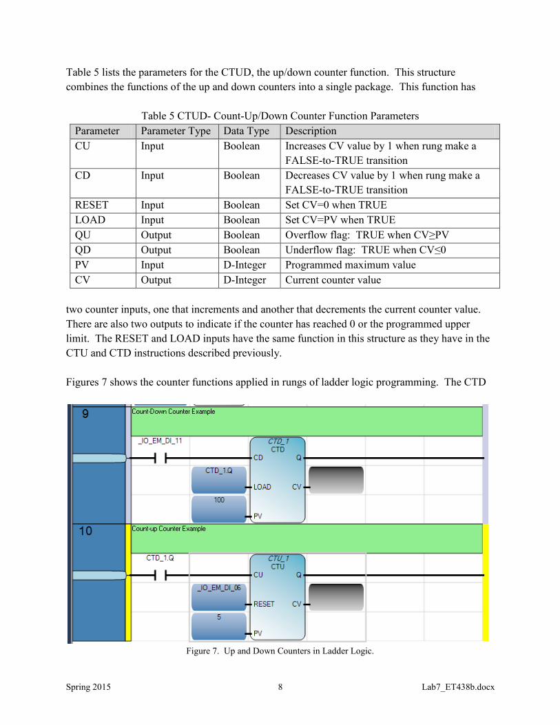
Figure 9 shows the state diagram for the example process. The diagram starts with an input from

the first scan variable of the PLC. This variable is TRUE only for the first PLC program scan

and places the process in the stop state. This guarantees that the process will be stopped even

after a power outage. From this point, the process progresses to the start state if the start push

button is pressed. Once in the start state, the process will transition to the tank filling state if the

float switch indicates the tank is empty. If the tank is empty, the control scheme opens the inlet

value allowing the tank to fill with mixture. The float switch detects a full tank and allows the

process to move to the mixing state. An output energizes the mixer motor after the process

enters this state. The mixing state continues until 20 minutes have elapsed, after which the

process enters into the tank draining state. In this state, the drain value is opened and the state

maintained until the float switch indicates the tank is empty. Pressing the stop push button at

each stage of the process ends the current operation and returns the system to the stop state.

S0

I0

1st scan

S1

I2

I1

Stop

Start

O0

Open

inletI3

Float

switch

closed

S2

S3

S4

I3O2

Float

switch

open

Mixer

Motor

Start

Tank

Filling

I2

Stop

Pressed

Start

Pressed

T=20 min

Mixing

Tank

Draining

I2+I3

O1

Open

outlet

Stop pressed or

float switch

I2

Figure 9. Example State Diagram Showing Transitions and Outputs


c.) State equations convert the state diagram into Boolean expressions relating the inputs to

states. The first step in developing state equations is to determine the coding of the states.

Individual bits can store the state variables. A number of bits, n, can store up to 2n states. The

number of states in this example is five so three bits can store all the defined states. Table 6

shows one way to code the states for this example. A selected code should attempt to only

Table-6 Coding of States In Example Problem

X1 X2 X3 Diagramed State Identifier

0 0 0 S0: Stopped State

0 0 1 S1: Start State

0 1 0 S2: Tank Filling

0 1 1 S3: Mixing State

1 1 1 S4: Tank Draining

change the value of single bit as the program transitions among the defined states. This

simplifies the transitional Boolean equations. Another coding method assigns a single bit to each

state. Table 7 shows this coding. This method does not take advantage of the fact the each bit

can store two states and is quite wasteful of resources. It is easier to understand since each bit

Table-7 Coding of States In Example Problem

S0 S1 S2 S3 S4 Diagramed State Identifier

1 0 0 0 0 S0: Stopped State

0 1 0 0 0 S1: Start State

0 0 1 0 0 S2: Tank Filling

0 0 0 1 0 S3: Mixing State

0 0 0 0 1 S4: Tank Draining

represents a condition of the system process and it is either in the state (1) or out of the state (0).

This example uses the coding from Table 7.

Examining the state diagram and utilizing the general form of the state equations given in (1) and

(2) produces the system of Booleans state equations show in equations 3a-3e.

2I3I3S)T,3S(TON4S4S .)e

2I)T,3S(TON2S3I3S3S .)d

3I2I1S3I2S2S .)c

3I2I0S1I1S1S b.)

2I4S3I2I0I0S0S a.)

(3)


These equations combine memoryless and retained state memory in their implementation. The

set conditions are enclosed in the square brackets and the reset conditions follow the terms

enclosed in the brackets.

Output equations relate the inputs and states to the desired output actions. Using a single bit to

indicate a state makes the output equations simple. Equations (4) give the output relationships

for the example.

mixer)(Start 3S2O

drain)(Open 4S1O

inlet)(Open 2S0O

(4)

d.) Converting the state equations to a PLC program requires the specification of the input and

output points on the controller and the type of switch contact employed. Table 8 lists the I/O

points used in this example.

Table-8 PLC I/O Point Assignments

Inputs

I1 Start (N.O. contact) DI_00

I2 Stop (N.C. contact) DI_02

I3 Float Switch (N.C. contact) DI_03

Outputs

O0 Open Inlet DO_00

O1 Mixer Motor Start DO_02

O2 Open Outlet DO_01

The state equations produce the rungs of the ladder program with some modifications. The

conditions of the specified external contacts (N.O.=normally open and N.C. normally closed)

will control the logic. A NOTed variable in the state equations my translate into a direct contact

in the PLC program. The goal is to maintain the logical continuity of the rung not electrical

continuity.

The state equation structure assumes that they are computed simultaneously. Remember that the

PLC executes a program from top down and left to right so state equations are not updated in

parallel. Adding intermediate state variables allow state equations to re-compute correctly.

This example defines S0X, S1X, S2X, S3X, and S4X as the intermediate state variables. The

state variable updates should appear after all state equations in the ladder program structure. Any

timers or counter that depend on state variable changes follow the updates. The final section

should be the output equations. Figure 10 shows the Connected Components Workbench ladder

diagram program file printout for this example. This section is the ladder diagram for the five


state equations. Logical OR functions in the state equations become parallel contacts in the

ladder program while the AND functions become series contacts. The outputs are the

intermediate variables discussed above.. These are user defined bits in memory of a Boolean

type.

Figure 10. PLC Ladder Diagram for Example State Equations.

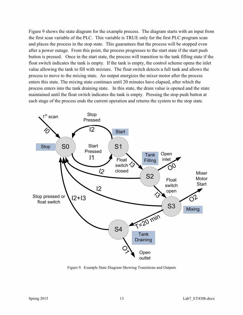
Figure 11 shows the section of ladder diagram program code that updates the state variables after

their values are recomputed by the state equations shown above. These are very simple

statements in which a direct contact associated with the intermediate variable changes the bit

values of the direct coil instructions whenever the intermediate variable changes. These rungs

should appear after the state equations in a ladder program for proper operation.


Figure 12 shows the last section of the program. This section includes the timer function

actuated by state variable S3 and the output equations. The output equations are very simple.

They relate the state variables to the desired physical output points. The timer rung is the last

rung in the program and is set to 10 seconds to test the program.

Figure 11. State Variable Updates For Example Problem.

Figure 12. Output And Timer Equations For Example Problem.


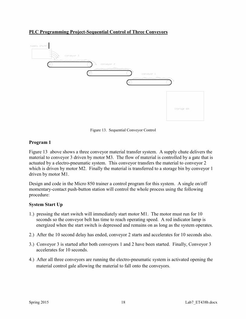
PLC Programming Project-Sequential Control of Three Conveyors

Figure 13. Sequential Conveyor Control

Program 1

Figure 13 above shows a three conveyor material transfer system. A supply chute delivers the

material to conveyor 3 driven by motor M3. The flow of material is controlled by a gate that is

actuated by a electro-pneumatic system. This conveyor transfers the material to conveyor 2

which is driven by motor M2. Finally the material is transferred to a storage bin by conveyor 1

driven by motor M1.

Design and code in the Micro 850 trainer a control program for this system. A single on/off

momentary-contact push-button station will control the whole process using the following

procedure:

System Start Up

1.) pressing the start switch will immediately start motor M1. The motor must run for 10

seconds so the conveyor belt has time to reach operating speed. A red indicator lamp is

energized when the start switch is depressed and remains on as long as the system operates.

2.) After the 10 second delay has ended, conveyor 2 starts and accelerates for 10 seconds also.

3.) Conveyor 3 is started after both conveyors 1 and 2 have been started. Finally, Conveyor 3

accelerates for 10 seconds.

4.) After all three conveyors are running the electro-pneumatic system is activated opening the

material control gale allowing the material to fall onto the conveyors.


System Shut Down

1.) The stop push button is depressed.

2.) The flow of material though the gate is stopped by closing it.

3.) All motors must continue to run for 30 seconds to clear material from the conveyor belts.

After this time delay all motors are de-energized and a green indicator lamp lights to show

that the system is stopped. This light will remain on after the push button is released. It goes

out when the start button is pressed.

Use the following I/O assignments on the trainer and develop a PLC program to implement this

control.

DI0 (N.O. switch) start DO2 red run lamp

DI2 (N.C. switch) stop DO4 green stop lamp

_SYS_T_SCAN=First Scan Bit DO5 conveyor motor 3

DO3 conveyor motor 2

DO1 conveyor motor 1

DO7 material gate open

Program 2

To save wear on the conveyor system, the above control is modified to shut down each conveyor

in sequence as it empties. Tests show that conveyor 3 takes 7 seconds to clear, conveyor 2 takes

9 seconds to clear, and conveyor 1 takes 14 seconds to clear.

Modify the first program to cause the conveyors to shut down in the sequence 3-2-1 after the

gate is closed with the time delays required to clear each belt.

Lab 7 Assessment

Complete and submit the following items for grading and perform the listed actions to complete

this laboratory assignment.

1.) Complete the online quiz over Lab 7 technical background.

2.) Develop a state transition diagrams for programs 1 and 2

3.) Write Boolean state equations for programs 1 and 2

4.) Code programs 1 and 2 into the PLC trainer

5.) Demonstrate working programs to the lab TA

6.) Submit pdf files of the working programs, the developed state diagrams, and the state

equations to the dropbox for lab 7

Documents

ET 438B Sequential Control and Data Acquisition … · Sequential Control and Data Acquisition Laboratory 7 PLC Function Programming Using Ladder Logic ... Write Boolean state equations