LINKÖPING 2008

STATENS GEOTEKNISKA INSTITUTSWEDISH GEOTECHNICAL INSTITUTE

Repo

rt 73

Estimation of pore pressure levelsin slope stability calculations:Analyses and modelling of groundwaterlevel fluctuations in confined aquifersalong the Swedish west coast

HÅKAN PERSSON

Swedish Geotechnical InstituteSE-581 93 Linköping

Information service, SGITel:+46 13 20 18 04Fax:+46 13 20 19 09E-mail: info@swedgeo.seInternet: www.swedgeo.se

0348-0755SGI-R--08/73--SE

Report

Order

ISSNISRN

T H E S I S F O R T H E D E G R E E O F L I C E N T I AT E O F E N G I N E E R I N G

Estimation of pore pressure levels in slope stabili tycalculations: Analyses and modelling of groundwater

level fluctuations in confined aquifers along theSwedish west coast

H Å K A N P E R S S O N

D e p a r t m e n t o f C i v i l a n d E n v i r o n m e n t a l E n g i n e e r i n g

D i v i s i o n o f G e o E n g i n e e r i n g

C H A L M E R S U N I V E R S I T Y O F T E C H N O L O G Y

G ö t e b o r g , S w e d e n 2 0 0 8

Estimation of pore pressure levels in slope stability calculations: Analyses and modelling of groundwater level fluctuations in confined aquifers along the Swedish west coast HÅKAN PERSSON © HÅKAN PERSSON, 2008 ISSN 1652-9146 Lic 2008:11 Department of Civil and Environmental Engineering Division of GeoEngineering Chalmers University of Technology SE-412 96 Göteborg Sweden Telephone + 46 (0)31 772 10 00 www.chalmers.se Chalmers reproservice Göteborg, Sweden 2008

iii

iv

ABSTRACT

The stability of clay slopes often depends on the current pore pressure levels, where high pressure levels are associated with low stability. In Sweden there is a recommended method for estimating the maximum pressure levels but for various reasons, discussed further in the thesis, this method has not become established. In this study several areas of improvement for the method recommended have been identified. Further, a classification system for groundwater level fluctuations in confined aquifers is presented. The classification is based on commonly available topographical and geological information and has been developed from analyses and simulations of groundwater level fluctuations in three study areas on the Swedish west coast. The model used in this study is a slightly modified version of the hydrological HBV model. Even though the use of the modified HBV model, for the purpose of groundwater level calculation, involves a highly conceptual description of the processes involved, the simulation results are promising. Calibration simulations show that the observed groundwater level variations in confined aquifers can be described satisfactorily. Furthermore, validation simulations show that even with little hydrogeological information of an area, groundwater levels can be simulated reasonably correctly using the model. In addition, preliminary climate change simulations, using the modified HBV model, indicate that the overflows in the confined aquifers govern the maximum levels, meaning that increased precipitation has limited influence on the groundwater levels. These simulations should, however, not be interpreted as predictions but more as an indication of an area of application for the model.

Keywords: landslide, slope stability, pore pressure, groundwater level, HBV model, confined aquifer, climate change

v

ACKNOWLEDGMENTS

A big thank you to my supervisors Claes Alén, Torbjörn Edstam and Karin Lundström, as well as to the project leader Bo Lind and the reference group with representants from Räddningsverket, Formas, Banverket, Vägverket, SMHI, SGU, Göteborgs Universitet, Chalmers and SGI. Not to forget the financiers: Räddningsverket, Formas, Banverket, Vägverket and SGI! And an extra thank you to colleagues at Chalmers and SGI. tomorrow is tuesday wonderland Asperögatan, Monday, 15 December 2008 Håkan Persson

vi

vii

TABLE OF CONTENTS

ABSTRACT ...............................................................................................................................IV

ACKNOWLEDGMENTS.........................................................................................................V

TABLE OF CONTENTS ........................................................................................................VII

LIST OF NOTATIONS .............................................................................................................X

1 INTRODUCTION ......................................................................................................... 13

2 HYDROGEOTECHNICS: WATER AND GEOLOGY RELATED TO

GEOTECHNICAL PROBLEMS ............................................................................... 15 2.1 Precipitation-induced landslides...............................................................16

2.1.1 Prediction methods.........................................................................17 2.2 Landslides and climate change .................................................................18 2.3 Geology of the fine sediment areas along the Swedish west coast.......19

3 THEORETICAL BACKGROUND ............................................................................ 20 3.1 Hydrologic cycle and groundwater formations ......................................21

3.1.1 Swedish west coast groundwater formations ..............................22 3.2 Aquifer properties......................................................................................23 3.3 Groundwater flow ......................................................................................26

3.3.1 Analytical solutions........................................................................27 3.4 Soil stress and strength concepts ..............................................................28

3.4.1 Drained and undrained conditions...............................................28 3.5 Soil consolidation .......................................................................................31

4 GROUNDWATER AND PORE PRESSURE DISTRIBUTION AND

FLUCTUATION ............................................................................................................ 32 4.1 Pressure levels.............................................................................................34 4.2 Pressure profiles .........................................................................................36

4.2.1 Stability effects of different pressure profile changes ................37 4.3 Pressure fluctuation ...................................................................................38

4.3.1 Non-infiltration causes of fluctuation ..........................................43

5 MODELLING AND PREDICTION OF GROUNDWATER LEVELS................. 43 5.1 The HBV model .........................................................................................44

5.1.1 Snow routine ...................................................................................45 5.1.2 Soil routine ......................................................................................45

viii

5.1.3 Response function ..........................................................................46 5.1.4 The Harestad model.......................................................................48

5.2 SEEP............................................................................................................48 5.3 The Chalmers model..................................................................................49

5.3.1 Model strengths and areas of improvement................................52 5.3.2 Maximum pressure levels ..............................................................53

6 DEVELOPMENT OF THE MODIFIED HBV MODEL .......................................... 55 6.1 Model structure ..........................................................................................56 6.2 Model parameters ......................................................................................58 6.3 Physical interpretation of the model........................................................60

7 STUDY AREAS AND AVAILABLE DATA .............................................................. 62 7.1 Maps, precipitation and temperature ......................................................64 7.2 Groundwater levels and pore pressures ..................................................64

8 ANALYSES OF GROUNDWATER LEVEL OBSERVATIONS......................... 65 8.1 Fluctuation patterns ...................................................................................66 8.2 Accuracy of the open standpipe measurements .....................................69 8.3 Quality and functionality of the Groundwater Network.......................72

9 RESULTS FROM SIMULATIONS USING THE MODIFIED HBV MODEL.... 75 9.1 A revised classification system for groundwater level fluctuations .....76 9.2 Sandsjöbacka ..............................................................................................77

9.2.1 Model calibration ...........................................................................77 9.2.2 Classification and model parameter evaluation..........................79 9.2.3 Model validation.............................................................................80

9.3 Harestad ......................................................................................................83 9.3.1 Model calibration ...........................................................................84 9.3.2 Classification and model parameter evaluation..........................85 9.3.3 Model validation.............................................................................87

9.4 Brastad.........................................................................................................89 9.4.1 Model calibration ...........................................................................90 9.4.2 Classification and model parameter evaluation..........................91

9.5 Experiences from the calibration and validation of the modified HBV model.....................................................................................................................92

10 POSSIBLE INFLUENCE OF CLIMATE CHANGE .............................................. 94

11 CONCLUSIONS.......................................................................................................... 99 11.1 Practical implications ...............................................................................101 11.2 Future work...............................................................................................102

ix

12 REFERENCES............................................................................................................104

x

LIST OF NOTATIONS

The following notations are used in the thesis: Notation Description Unit

A amplitude for yearly evapotranspiration variation

-

B(t) evaporation factor mm/(day·˚C)

c cohesion kPa

ccons consolidation coefficient m2/s

CE evapotranspiration factor mm/(day·˚C)

CM melting factor mm/(day·˚C)

D diffusivity m2/s

EA actual evapotranspiration mm

EP potential evapotranspiration mm

ep 'effective porosity' -

FC field capacity mm

IN infiltration mm

k hydraulic conductivity m/s

klz proportionally constant for the bottom outflow from lz

1/day

klz,overflow proportionally constant for the overflow outflow from lz

1/(mm·day)

kuz proportionally constant for the bottom outflow from uz

1/day

kuz,overflow proportionally constant for the overflow outflow from uz

1/day

llz,overflow level for the overflow outflow from lz

mm

LP soil moisture level for which EA reaches EP

mm

lz (level in) lower groundwater reservoir

mm

M oedometer modulus kN/m2

n porosity -

Pmax maximum level in the prediction station during the observation period

cm rel. to g.l.

200maxP maximum level in the prediction

station with a return period of 200 years

cm rel. to g.l.

qlz bottom outflow from lower groundwater reservoir

mm/day

xi

quz bottom outflow from upper groundwater reservoir

mm/day

quz,overflow overflow outflow from upper groundwater reservoir

mm/day

R recharge mm

rP variation in the groundwater level in the prediction station during the observation period

cm

rR variation in the groundwater level in the reference station during the observation period

cm

S storativity -

SM soil moisture mm

200RS |

200maxy -ymax|

cm

Sret specific retention -

Ss specific storativity 1/m

Ss,clay specific storativity for clay 1/m

Sy specific yield -

T transmissivity m2/s

T air temperature ˚C

TT threshold air temperature ˚C

u pore pressure kPa

uz (level in) upper groundwater reservoir

mm

ymax maximum level for the reference station during the observation period

cm rel. to g.l.

200maxy maximum level for the reference

station with a return period of 200 years

cm rel. to g.l.

zgw groundwater level cm rel. to g.l.

zmax highest observed groundwater level

cm rel. to g.l.

zmin lowest observed groundwater level

cm rel. to g.l.

β factor controlling the shape of the recharge curve

-

βs compressibility of the bulk soil material

m2/kN

βw compressibility of water m2/kN

γw unit weight of water kN/m3

∆t time delay in the response function

day

σ total stress kPa

σ' effective stress kPa

xii

τ shear strength kPa

Φ' friction angle ˚

ψ phase offset for evapotranspiration

day

13

1 INTRODUCTION

Areas in Sweden with the prerequisites for landslides are in general moderately sloped clay areas or relatively steep sandy or silty slopes (2008). Many slope failures occur in man-made constructions such as road embankments or excavations. Failures in areas unaffected by construction work or deep foundations generally occur beside streams and rivers. In sandy and silty slopes the size of an individual landslide is generally small, even though the long-term effect of a continuous sliding and erosion process can be severe. On the other hand, major landslides occur mainly in clay areas, especially where quick clay is present (SRV, 2008). In areas with unsatisfactory stability and in connection with the design of new infrastructure (roads, buildings etc.), slope stability investigations are carried out. When investigating slope stability, pore pressures in a specific slope must be considered since the highest risk of slope failure often coincides with the highest pore pressures. In situations where the undrained1 shear strength governs the soil strength, the pore pressure, however, is irrelevant. Nevertheless, the risk of failure under drained conditions must be considered in all slope stability investigations. Consequently, the level of maximum pore pressure that is expected to occur within a certain design period needs to be estimated. At present there is no established standard for how prediction of maximum pore pressures should be carried out. A common method is to calculate the pore pressure conditions required for a specific slope to fail, compare these calculated pressures with observations of local conditions and consider whether the calculated pressures are reasonable. Another estimation method is to add a 'safety margin', based on experience, to observed pore pressures. Both these approaches are commonly used in Sweden according to Johansson (2006). Even though there is no established standard for the calculation of maximum pore pressures, there is a method recommended by both the Swedish Commission on Slope Stability (CoSS, 1995) and in the Eurocode2 for slope stability calculations. The basis of this method is statistical treatment of long series of groundwater level measurements from a nationwide network of reference areas (Svensson,

1 A failure in soil can occur under either drained or undrained conditions, and is further discussed in Chapter 3.4.1. 2 Can be found in Eurocode 7, part 2, BS EN 1997-2

14

1984). For various reasons, mainly related to prediction limitations and handling difficulties, the method is not commonly used. The recommended method for predicting maximum pore pressures has been developed primarily for clay areas. However, the processes that cause stability problems due to high pore pressures differ considerably between sandy or silty slopes and clay areas. In Sweden, clay areas are common in a zone from Gothenburg on the west coast to Stockholm on the east coast and also along most of the coastline. This study focuses on analyses of groundwater pressures in clay areas in the Swedish west coast region, near Gothenburg, where the softest3 clay is also present. Moreover, this study considers natural areas as opposed to areas with dense construction work and deep foundations. Pore pressures in a clay slope are governed by hydrogeological boundary conditions. If the water pressures below and above the clay are known, the pore pressures within the clay can be calculated. Even though the actual pore pressures are discussed in this study, the main focus is on the boundary conditions constituted by groundwater levels4 in the friction material below the clay, i.e. the water pressure in confined aquifers. In order to improve our understanding of groundwater systems in clay areas, groundwater level fluctuations in confined aquifers have been analysed and simulated. Furthermore, an attempt has been made, to identify typical examples of these fluctuations, based on objective criteria such as local topography, geology and position within an aquifer. Apart from analyses and simulations of groundwater fluctuations, the recommended method for maximum pore pressure predictions has also been analysed and tested. Consequently, extended studies of the superficial groundwater systems is a remaining and important part of future research. The groundwater level analyses and simulations carried out resulted in general criteria governing the fluctuation patterns and the simulation results appear promising despite the fact that a highly conceptual model has been used. This licentiate thesis presents partial results from a larger ongoing research project. The overall aim of this larger project is to improve and develop methods for pore pressure prediction in slope stability calculations, taking into account climate change. Due to climate change the weather in most parts of Sweden is expected to become wetter, resulting in estimated increases in precipitation and run-off of up to 30% (Rossby Centre, 2007). A wetter climate will most likely result in

3 Soft clay is clay with low shear strength. 4 The term 'groundwater level' is often used for the groundwater pressure level in friction materials, while the term 'pore pressure' is used for soils with low permeability, such as clay.

15

higher pore pressure levels and thus actualise further the need for maximum pressure predictions. Despite the fact that the climate change issue has brought the subject of this research project to the fore, predictions of pore pressures are also essential for reliable slope stability calculations in the present climate.

2 HYDROGEOTECHNICS: WATER AND GEOLOGY RELATED TO GEOTECHNICAL PROBLEMS

Many traditional geotechnical problems are related to the interaction between soil and water. However, knowledge of groundwater systems (including pressure levels and flows) among geotechnical engineers could be improved. Knowledge of surface water is considerable among hydrologists and knowledge of groundwater is considerable among hydrogeologists. If knowledge in these traditionally separate fields can be utilised this could increase substantially our knowledge of the interaction between soil and water in geotechnical problems. A suitable name for such utilisation could be hydrogeotechnics5. Geotechnical problems related to groundwater mainly concern settlement and stability. Lowered groundwater levels could cause settlement, while stability problems are generally related to high water levels or intense precipitation. This study deals primarily with stability problems related to high pore pressure and groundwater level in deep layers due to the long-term effects of infiltrated precipitation. Other types of water-induced slope stability problems can be attributed to heavy rain causing increased pore pressures in shallow layers, loading effects from superficially stored rain and surface or inner erosion (piping). Another example is riverbank erosion, which however can be regarded as a morphological process. An earlier study in the field of hydrogeotechnics is the PhD Thesis Hydrogeological Methods in Geotechnical Engineering (Persson, 2007), which focused on urban areas and the effects of construction work. The present study can in some ways be seen as a complement to (Persson, 2007), although oriented more towards stability in natural areas, i.e. not affected by construction work, rather than settlements in urban areas. Other works that are especially important

5 This term has been suggested by Claes Alén but has also been used in a few earlier, yet similar, cases.

16

for this study are the PhD theses Analys och användning av grundvattennivåobservationer by Svensson (1984) and Portrycksvariationer i leror i Göteborgsregionen by Berntsson (1983), which studied the behaviour of groundwater pressures in the Gothenburg region for aquifers and clay respectively.

2.1 Precipitation-induced landslides Precipitation can induce landslides in several ways, where the most obvious soil movements are perhaps debris flows (also called mud flows or earth flows). These debris flows are caused by erosion due to heavy rain and consist of water mixed with soil that flows, rather than slides, downhill (Wikipedia, 2008). Debris flows are common in areas with steep slopes and sparse vegetation. Shallow slides are often induced by high pore pressures in superficial layers. These high pressures are typically caused by precipitation or snowmelt infiltrating the uppermost soil layers. Shallow slides are also common in steep slopes, especially in areas where negative pore pressures are required for maintaining the stability of the slope. For the deep-seated slides in clay areas, which are the focus of this study, the direct effect of rainfall is not as obvious as it is for shallow landslides. The direct effect on the deep-layer pore pressures of increased groundwater levels in the uppermost soil layers often is small. However, the clay generally overlays friction material into which water can infiltrate and increase the groundwater pressure level. This increased groundwater pressure is spread through the clay layer and, especially for slip surfaces near the friction material layer, raises the pore pressures in the clay. However, for many deep-seated slides the present pore pressure level has no significant influence on stability since the conditions are undrained6. Research into rainfall-induced landslides has focused generally on shallow slides and debris flows and has received contributions from fields such as engineering geology, soil mechanics, hydrology and geomorphology (Guzzetti, 1998; Crosta, 2004; Crosta and Frattini, 2008). The research focus has varied between the different fields. The following is a state-of-the-art introductory text by (Crosta and Frattini, 2008)7:

"Engineering geologists have focused their attention on the effect of water infiltration

on soil strength and unsaturated conditions. At the same time, they have reported and

6 The theoretical background for pore pressure-induced slope failures is discussed in Chapter 3.4.1. 7 For references, see Crosta and Frattini (2008).

17

studied hundreds of case studies that have been fundamental for the understanding of

the problems.

Hydrologists have concentrated their efforts on the processes that control surface

and sub-surface storm-flow at the hill slope and catchment scale. Together with

geomorphologists, they have also contributed to the quantification of the topographic

controls on hydrological processes."

2.1.1 Prediction methods Prediction methods for landslides can, for example, aim at predicting when (and where) there is a risk of landslides, or predicting the lowest future stability for a specific slope. Measurement data used for prediction, except for information about topography and soil shear strength, are typically precipitation, soil moisture, groundwater levels and pore pressure. The scale of the methods can vary, from general e.g. for a climate region, to specific for a certain site where local geology thus needs to be considered. Development of warning systems for predicting landslides has focused on debris flows and shallow slides. The most commonly investigated rainfall parameters are: total 'cumulative' rainfall, antecedent8 rainfall, rainfall intensity and rainfall duration (Guzzetti et al., 2005). Various combinations of these parameters have also been tested. A synthesis of thresholds from several investigations of intensity-duration studies is shown in Figure 2.1, which indicates a wide span of triggering levels.

8 Antecedent, synonym for previous, is often used in the literature.

18

Figure 2.1 Synthesis of threshold levels for triggering landslides from several studies carried out

worldwide. The threshold levels indicate the lowest combination of rainfall intensity and duration for a landslide to begin. Note the wide span of estimated threshold levels. Figure adopted from Guzzetti et al. (2005).

Detailed models describing specific sites have also been developed. Quasi-three-dimensional hydrological models for predicting landslides have been created by e.g. Terlien (1998) and Malet (2005). Terlien also discusses deep slides, for which a hydrological model is used to determine the pore pressures. The study, however, focuses on sandy and silty soils. Moreover, the model for prediction of maximum pore pressures, mentioned above, has been developed by Svensson (1984) and was complemented in CoSS (1995). Modelling of groundwater levels has been done in several hydrological studies, but generally without aiming at predicting landslides (see Chapter 5).

2.2 Landslides and climate change A preliminary Swedish study found that during a period with precipitation that is 40% above mean the groundwater levels in the area studied rose by up to 0.9 m (Hultén et al., 2005). Stability calculations of some clay slopes along the Göta Älv river in Sweden indicate that the safety factor may decrease by a few per cent as the pore pressure increases due to the increase in precipitation. This decrease in safety factor can be highly significant when the slope is barely stable (Hultén et al., 2005). The impact of climate change on slope stability has been identified in

19

many parts of the world, eg by Buma (2000), Dehn et al. (2000) and McInnes et al. (2007). For the type of slope stability problems this study is focusing on, the determining factors for stability are the maximum groundwater levels and pore pressures. Consequently, assessments carried out by hydrologists of the change in groundwater level due to climate change are also highly relevant in this context.

2.3 Geology of the fine sediment areas along the Swedish west coast

Characteristic of the geological formations along the Swedish west coast is the occurrence of bedrock areas, either bare or covered with thin till soils, rising high above the surrounding valleys with fine sediment soils. The level difference between the highest bedrock level and the valley bottom is often 100 m or thereabouts. The quaternary deposits in western Sweden are a result of the latest glaciations' withdrawal from the area. The occurrence of till is more limited on the west coast than in the rest of Sweden and if present it is often covered with fine marine sediments (Berntsson, 1983). Principal soil profiles for the Swedish west coast are illustrated in Figure 2.2 and Figure 2.3.

Figure 2.2 Typical soil stratification for the Swedish west coast region; from Cato and Engdahl

(1982).

20

Figure 2.3 Typical soil stratification for a valley in the Swedish west coast region; modified from

Berntsson (1983).

In Figure 2.3 a zone in the upper part of the clay can be distinguished. In this zone, called the dry crust, the clay is affected considerably by exposure to drying, weathering, frost, chemical processes, vegetation and biological activity. These processes cause the development of cracks and macro-pores. The lower part of the dry crust is also affected by thin (1-5 mm) but continuous cracks to a depth of up to 5-10 m (Berntsson, 1983). The cracks increase the hydraulic conductivity of the dry crust substantially. In a study in Skara, Sweden, it was found that these cracks contained enough water to supply a village of 7,000 people (Berntsson, 1983). Important geological deposit formations with regard to groundwater formations also include the occurrence of sand and silt layers within the clay deposits, which can contribute substantially to horizontal groundwater flow.

3 THEORETICAL BACKGROUND

To simplify the reading of this report, some of the most important concepts of hydrogeotechnics involved in this study are explained in this chapter. Since a wide range of subjects are covered, not all concepts are explained in detail. For more background information and detailed explanations see textbooks from each traditional academic field, e.g. Freeze and Cherry (1979), Chow et al. (1988), Terzaghi et al. (1996) and Sällfors (2001), on which this chapter is based. The academic fields of hydrogeology and geotechnical engineering have a great deal in common but in many cases the parameters used to describe the same phenomena are different. An attempt to bridge this difference can be found in Persson (2007).

Dry crust clay

Bedrock

Clay

Gravel

21

3.1 Hydrologic cycle and groundwater formations The circulation of water between rivers, lakes, oceans, the atmosphere and the ground is usually referred to as the hydrologic cycle (see Figure 3.1). The driving mechanism in this circulation is radiation from the sun. This radiation causes water evaporation and plant transpiration, which together are called evapotranspiration. At high altitude the evapotranspiration is cooled down and condenses into water droplets, which eventually cause precipitation. When precipitation falls as snow, water is stored in the snowpack and the circulation is delayed until snowmelt. Precipitation falling as rain, or melting snow, causes run-off into streams, lakes and oceans as well as recharge into groundwater reservoirs. On average over a large area, the infiltration is caused by precipitation minus evapotranspiration and is called the effective precipitation. Looking at the infiltrating water and the groundwater reservoirs in detail, a more correct name for the hydrologic cycle could be the hydrogeological (or geohydrological) cycle.

Figure 3.1 The principal flows in the hydrologic cycle; from Todd (1959).

A geologic deposit that has sufficient hydraulic conductivity for considerable quantities of water to be stored and withdrawn from wells is called an aquifer. An aquitard, on the other hand, is a geologic deposit that is not permeable enough to transmit a significant amount of water. Aquifers can be classified into two main types: unconfined and confined (see Figure 3.2). An unconfined aquifer is a layer of quite highly permeable soil extending to the ground surface and with a free water table at some level within

22

the soil layer. The uppermost limit for an unconfined aquifer is the free water table. A confined aquifer is formed from a quite highly permeable soil covered by an impervious soil, stopping groundwater from flowing vertically. When the confining soil layer is not impervious, but still has a low permeability, the underlying aquifer is regarded as 'leaking'. Normally, there is no free water table within a confined aquifer. However, in a well that penetrates the confining layer the groundwater pressure level can be measured as a free water table. This water level can reach above the ground level and the aquifer is then called artesian. The maximum pressure level the groundwater in a confined aquifer can reach is governed by overflow levels in the recharge areas, i.e. the maximum level of the confining stratum (see Figure 3.2).

Figure 3.2 Principal classification of confined and unconfined aquifers with accompanying

groundwater pressure levels; modified from Todd (1959).

Recharge into aquifers is governed by the fact that water infiltration mainly occurs in coarse, permeable soil or fractured rock. Recharge into unconfined aquifers can occur over the entire aquifer area and the main direction of flow in the aquifer is vertical. Recharge into confined aquifers, however, only occurs in small areas along the aquifer edges. In these recharge areas the flow direction is vertical whilst in the main part of the aquifer the flow is more or less horizontal. The recharge area of a confined aquifer can be considered to be an unconfined aquifer.

3.1.1 Swedish west coast groundwater formations A typical soil profile in the clay areas along the Swedish west coast can be characterised according to Figure 3.3. The uppermost meter of the clay dry crust, with a strongly cracked structure, is called the upper aquifer. It is characterised by high permeability and thus rapid pore pressure responses. The maximum groundwater level in this zone normally equals ground level. In the lower part of

23

the dry crust the cracks also govern the groundwater behaviour, resulting in rather rapid pore pressure responses. Since the cracks are mainly vertical, the horizontal permeability is generally9 low and the zone is referred to as Aquitard I. Aquitard II is the underlying zone with homogeneous clay and low permeability. In the lowest zone, the confined aquifer, the permeability is high and pressure responses are rapid.

Figure 3.3 Principal soil stratification and aquifer/aquitard classification for clay areas along the

Swedish west coast; modified from Berntsson (1983).

3.2 Aquifer properties In a soil material the actual soil material particles only constitute a part of the total soil volume, while the rest is normally water and/or air. This property is described by the porosity:

tot

airwater

V

VVn

+= (3.1)

where n = porosity [-] Vwater = volume of water [m3] Vair = volume of air [m3] Vsoil = total soil volume [m3]

If the water table in an unconfined aquifer is lowered, some of the soil that was saturated and below the groundwater table will be situated above the groundwater table and will therefore also be drained. The amount of water

9 In the area where 7,000 people were supplied with water from the dry crust, mentioned in Chapter 2.3, the horizontal hydraulic conductivity must be rather high.

Dry crust clay

Clay with small cracks

Homogenous or layered clay

Friction material

Upper aquifer

Aquitard I (hydrostatic)

Aquitard II

Lower aquifer

24

drained from the soil depends on the soil material and a measure of this property is called the specific yield. Specific yield is defined as the ratio between the volume of water that drains from a saturated soil volume, due to gravity, and the total volume of the soil. The amount of water that remains in the soil after gravitational drainage is likewise measured using a parameter called specific retention. The sum of specific yield and specific retention equals the porosity, so that:

nSS rety =+ (3.2)

where Sy = specific yield [-] Sret = specific retention [-]

Within the field of hydrology, the specific retention is often (for a certain soil depth) called field capacity. The amount of water that an aquifer can transport is related to the hydraulic conductivity10 of the aquifer material but also to the thickness of the aquifer. This property is called transmissivity:

kbT = (3.3)

where T = transmissivity [m2/s] k = hydraulic conductivity [m/s] b = thickness of aquifer [m]

A change in hydraulic head will, however, also affect confined aquifers and saturated parts of an unconfined aquifer. Water pressure changes cause soil skeleton reconfiguration resulting in water storage or expulsion depending on the direction of the pressure change. A rise in water pressure will expand the soil skeleton while a pressure drop will cause contraction. In hydrogeology this property is referred to as elasticity although strictly speaking the deformations can also be plastic. Expressed in geotechnical terms these phenomena equal swelling and consolidation respectively. The reason for compaction or expansion of the soil skeleton is the fact that increased water pressure causes decreased soil skeleton forces, which can be described as the Archimedes principle applied in soil. In geotechnical engineering the concept of effective stress is commonly used and for saturated conditions it can be expressed as:

u−= σσ ' (3.4)

where σ' = effective stress [kPa] σ = total stress [kPa] u = water pressure [kPa]

10 Often referred to as permeability in geotechnical engineering.

25

Furthermore, increased water pressure will cause water contraction and inversely decreased pressure will cause water expansion. This means that as the hydraulic head is lowered, contraction of the soil skeleton will reduce the porosity and expel water. In addition, the pore water will expand and release additional water. The parameter describing water storage or expulsion due to pressure change is called storativity and is the volume of water that will be stored or released per unit of surface area of the aquifer per unit change in water pressure head:

( )sww nbS ββγ += (3.5)

where S = storativity [-] γw = unit weight of water [kN/m3] b = thickness of the aquifer [m] n = porosity [-] βw = compressibility of water [m2/kN] βs = compressibility of the bulk soil material [m2/kN]

The parameter specific storage is also used, which is the storativity per unit thickness of the aquifer:

( )swws nb

SS ββγ +== (3.6)

where Ss = specific storativity [1/m]

The compressibility of water is 4.4·10-7 m2/kN, which can be compared with the compressibility for aquifers, which is about 10-6 to 10-2 m2/kN (Kruseman and de Riddler, 1970) and for normally consolidated glacial clays about 10-3 to 10-

2 m2/kN (Persson, 2007). Consequently, the compressibility of water is negligible for normally consolidated glacial clays and the specific storativity for the clay can thus be written as:

swclaysS βγ=, (3.7)

where Ss,clay = specific storativity for clay (negligible compressibility of water) [1/m]

The compressibility of a soil is in geotechnical engineering normally described using the oedometer modulus, which can be related to the compressibility as:

sswnM

βββ11 ≈

+= (3.8)

where M = oedometer modulus (=Eoed) [kN/m2]

The rate of change in hydraulic head, e.g. at consolidation or water pressure fluctuations, is related to the compressibility of the soil and is further described in Chapter 3.3. In geotechnical engineering the consolidation coefficient is normally used to determine this effect:

26

wcons

kMc

γ= (3.9)

where ccons = consolidation coefficient [m2/s]

In hydrogeology the more general parameter diffusivity is used, which is identical to the consolidation coefficient when the compressibility of water is negligible:

ckMk

S

k

S

k

S

TD

wswclayss

===≈==γβγ,

cons (3.10)

where D = diffusivity [m2/s]

The diffusivity in hydrogeology, however, is generally used in the horizontal direction while in geotechnical engineering the consolidation coefficient is mainly used in the vertical direction.

3.3 Groundwater flow This study is focused on confined aquifers and consequently only groundwater flows in saturated conditions are studied. The principles for flow in unsaturated conditions are essentially the same although due to the effects of varying degrees of saturation they are more complicated to handle. In an unconfined aquifer the thickness of the saturated zone varies as the groundwater level varies. The transmissivity of an unconfined aquifer therefore depends on the groundwater level. This introduces further complexity to the groundwater flow analysis and the groundwater flow equation is described using the Boussinesq equation (e.g. Fetter, 1994). Groundwater flow in unconfined aquifers will, however, not be discussed further in this thesis. The general equation for groundwater flow in saturated conditions is derived from two fundamental principles: the law of mass conservation and the linear flow equation called Darcy's law. Darcy's law can be written as:

dx

dhk

A

Q −= (3.11)

where Q = water flow [m3/s] A = cross-sectional area [m2] k = hydraulic conductivity [m/s] h = hydraulic head [m] x = distance co-ordinate [m]

Sometimes Q/A is called Darcy velocity, which corresponds to 'piston flow'. To find the real velocity for a single water molecule the effective porosity of the soil also needs to be considered. For very low gradients, Darcy's law is not valid and

27

this has been shown by, for example, (Hansbo, 1960). This phenomenon does not affect this study seriously and is therefore not discussed further. For three-dimensional conditions the general groundwater flow equation11 can be written as:

t

hS

z

hk

zy

hk

yx

hk

x szyx ∂∂=

∂∂

∂∂+

∂∂

∂∂+

∂∂

∂∂

(3.12)

where kx = hydraulic conductivity in the x-direction [m/s] (and likewise for the y- and z-directions)

h = hydraulic head [m] t = time [s]

In equation 3.12 it is assumed that all flow comes from compression or expansion of the aquifer. In reality, water is often added as leakage through the confining layer. For leaking aquifers a leakage rate is introduced in the groundwater equation 3.12. With homogeneous, isotropic soil the groundwater equation 3.12, or the diffusion equation as hydrogeologists sometimes call it, can be written as (choosing geotechnical parameters):

t

h

cz

h

y

h

x

h

vcons ∂∂=

∂∂+

∂∂+

∂∂

,2

2

2

2

2

2 1 (3.13)

3.3.1 Analytical solutions Groundwater flow through a confined aquifer is essentially one-dimensional. A steady state and one-dimensional version (only considering the x-direction) of equation 3.12 has the form:

0=

∂∂

∂∂

x

hk

x (3.14)

The solution to equation 3.14 indicates that the groundwater pressure level is proportional to the flow and the distance but inversely proportional to the cross-sectional area (aquifer thickness) and the hydraulic conductivity:

0hxAk

Qh +⋅−= (3.15)

where h = groundwater pressure level [m] Q/A = water flow/cross section area [(m3/s)/m2] k = hydraulic conductivity [m/s] x = distance co-ordinate [m] h0 = initial groundwater pressure level [m]

11 Assuming incompressible water and no source term.

28

In Figure 4.3 the effect on the pressure levels from varying aquifer thickness can be seen. For conditions with time-dependent boundaries, i.e. transient conditions, analytical solutions applicable for confined aquifers have been presented by e.g. Todd (1959) and Huisman (1972).

3.4 Soil stress and strength concepts To handle geotechnical problems related to changes in groundwater levels, and using today's methods, the concept of effective stress is a prerequisite. If the groundwater levels in an area are lowered below the normal levels the effective stress level in the soil will increase, causing compaction (or settlement) of the soil. A significant lowering of the water level can be caused by pumping, for irrigation for example, or through leakage into a deeper tunnel. On the other hand, when the groundwater level rises, the effective stress decreases and thus also the inter-particle forces, which affects the shear strength of the soil as:

( )'tan' φστ += c (3.16)

where τ = shear strength [kPa] c = cohesion [kPa] σ' = effective stress [kPa] Φ' = friction angle [˚]

Equation 3.16 thus indicates that the shear strength decreases when the effective stress decreases (or the water pressure increases). Lowered shear strength of the soil means that the stabilising forces in the slope decrease and that the stability of the slope decreases. On the other hand, if the effective stress is increased through loading, the effect of increased driving forces in the slope will dominate and result in decreased stability. In addition to the effective stress level, the soil strength is governed by the soil material and the geological (stress) history of the soil.

3.4.1 Drained and undrained conditions A soil that is subject to shear deformations will normally experience a volume change, which for a water-saturated soil results in a change in pore pressure. In a highly permeable soil a change in pore pressure can be neutralised through water drainage. In a soil with low permeability, such as clay, the drainage process is slow and shear deformations and failures can therefore often be regarded as occurring under undrained conditions (Sällfors, 2001). Under undrained conditions the soil volume is regarded as being constant during shear deformation. Figure 3.4 illustrates the fundamental stress paths from active

29

triaxial tests, both for drained and undrained conditions and for a heavily overconsolidated soil as well as for a slightly overconsolidated soil. In the illustration for a heavily overconsolidated soil, soil failure occurs at A, while the undrained failure occurs at B. For the slightly overconsolidated soil, A illustrates the stress path for undrained condition, while B illustrates the path for drained conditions. In all cases, soil failure occurs when the Mohr-Coulomb failure line is reached. However, at C the vertical stresses equal the pre-consolidation pressure, meaning that the distance CB will cause large deformations. These deformations are often too large to be acceptable and normally cause pore pressure generation, which in turn can also cause undrained failures (Sällfors, 1986). Consequently, the drained soil strength is lower than the undrained soil strength for highly overconsolidated soils, while the opposite is true for normally or slightly overconsolidated soils.

Figure 3.4 Principal stress paths from a triaxial test, for a highly overconsolidated soil (left) and for

a slightly overconsolidated soil (right), from Sällfors (1986). [Brottlinje (in Swedish) is the failure line, and in situ spänning (in Swedish) is in situ stress.]

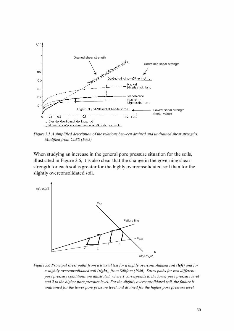
Sometimes, a simplified description for the relations between drained and undrained shear strengths is done, as illustrated in Figure 3.5. From the illustration it can be seen that the drained shear strength is expected to be governing the soil strength fro overconsolidation ratios in the range of 2-6.

30

Figure 3.5 A simplified description of the relations between drained and undrained shear strengths.

Modified from CoSS (1995).

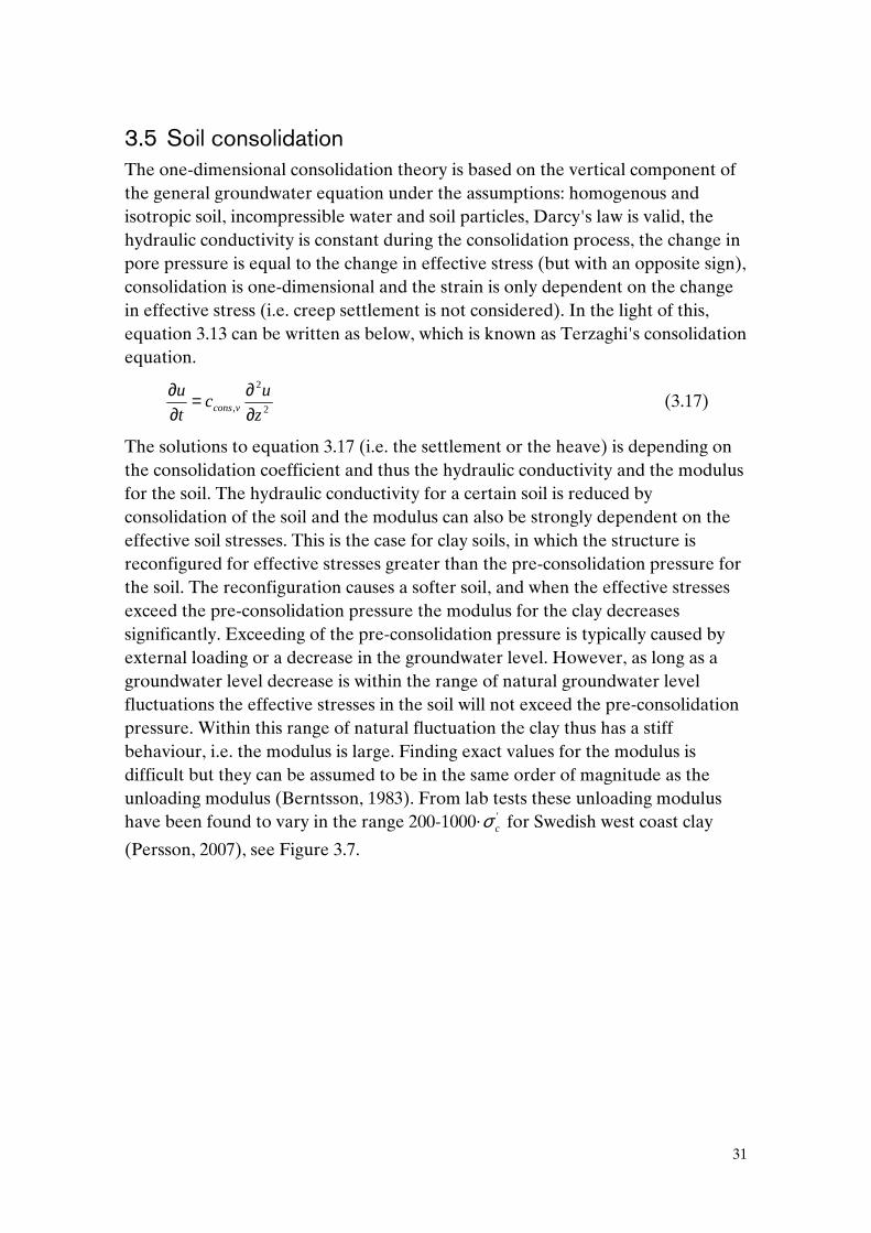
When studying an increase in the general pore pressure situation for the soils, illustrated in Figure 3.6, it is also clear that the change in the governing shear strength for each soil is greater for the highly overconsolidated soil than for the slightly overconsolidated soil.

Figure 3.6 Principal stress paths from a triaxial test for a highly overconsolidated soil (left) and for

a slightly overconsolidated soil (right), from Sällfors (1986). Stress paths for two different pore pressure conditions are illustrated, where 1 corresponds to the lower pore pressure level and 2 to the higher pore pressure level. For the slightly overconsolidated soil, the failure is undrained for the lower pore pressure level and drained for the higher pore pressure level.

σ'c,v

K0,nc

(σ'v-σ'h)/2

121 2

Failure line

(σ'v+σ'h)/2

Drained shear strength

Undrained shear strength

Lowest shear strength (mean value)

31

3.5 Soil consolidation The one-dimensional consolidation theory is based on the vertical component of the general groundwater equation under the assumptions: homogenous and isotropic soil, incompressible water and soil particles, Darcy's law is valid, the hydraulic conductivity is constant during the consolidation process, the change in pore pressure is equal to the change in effective stress (but with an opposite sign), consolidation is one-dimensional and the strain is only dependent on the change in effective stress (i.e. creep settlement is not considered). In the light of this, equation 3.13 can be written as below, which is known as Terzaghi's consolidation equation.

2

2

, z

uc

t

uvcons ∂

∂=∂∂

(3.17)

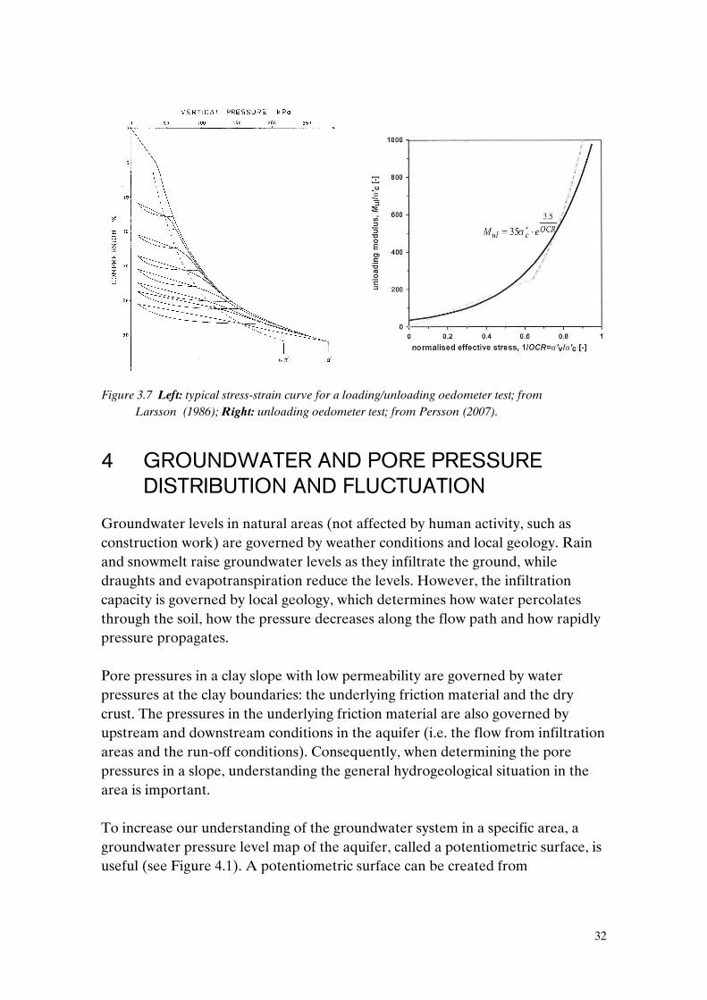
The solutions to equation 3.17 (i.e. the settlement or the heave) is depending on the consolidation coefficient and thus the hydraulic conductivity and the modulus for the soil. The hydraulic conductivity for a certain soil is reduced by consolidation of the soil and the modulus can also be strongly dependent on the effective soil stresses. This is the case for clay soils, in which the structure is reconfigured for effective stresses greater than the pre-consolidation pressure for the soil. The reconfiguration causes a softer soil, and when the effective stresses exceed the pre-consolidation pressure the modulus for the clay decreases significantly. Exceeding of the pre-consolidation pressure is typically caused by external loading or a decrease in the groundwater level. However, as long as a groundwater level decrease is within the range of natural groundwater level fluctuations the effective stresses in the soil will not exceed the pre-consolidation pressure. Within this range of natural fluctuation the clay thus has a stiff behaviour, i.e. the modulus is large. Finding exact values for the modulus is difficult but they can be assumed to be in the same order of magnitude as the unloading modulus (Berntsson, 1983). From lab tests these unloading modulus have been found to vary in the range 200-1000· '

cσ for Swedish west coast clay

(Persson, 2007), see Figure 3.7.

32

Figure 3.7 Left: typical stress-strain curve for a loading/unloading oedometer test; from

Larsson (1986); Right: unloading oedometer test; from Persson (2007).

4 GROUNDWATER AND PORE PRESSURE DISTRIBUTION AND FLUCTUATION

Groundwater levels in natural areas (not affected by human activity, such as construction work) are governed by weather conditions and local geology. Rain and snowmelt raise groundwater levels as they infiltrate the ground, while draughts and evapotranspiration reduce the levels. However, the infiltration capacity is governed by local geology, which determines how water percolates through the soil, how the pressure decreases along the flow path and how rapidly pressure propagates. Pore pressures in a clay slope with low permeability are governed by water pressures at the clay boundaries: the underlying friction material and the dry crust. The pressures in the underlying friction material are also governed by upstream and downstream conditions in the aquifer (i.e. the flow from infiltration areas and the run-off conditions). Consequently, when determining the pore pressures in a slope, understanding the general hydrogeological situation in the area is important. To increase our understanding of the groundwater system in a specific area, a groundwater pressure level map of the aquifer, called a potentiometric surface, is useful (see Figure 4.1). A potentiometric surface can be created from

33

groundwater level measurements in existing wells, together with new groundwater stations12 where additional information is required. Using this type of map a brief understanding of the geology, groundwater flows and aquifer properties can be achieved. From Darcy's law it follows that the flow is in the direction of the groundwater surface gradient and is thus perpendicular to the equipotential lines. The relative distance between the equipotential lines is a measure of the variations in flow resistance (i.e. the transmissivity). For an aquifer section with a certain flow, sparsely spaced lines indicate small friction losses, and thus low flow resistance (or high transmissivity), while areas with tightly packed lines indicate large friction losses.

Figure 4.1 A potentiometric surface with arrows indicating the flow directions, adopted from

Häggström (1988).

From a potentiometric surface, sections indicating the groundwater levels can also be extracted, as shown in Figure 4.2.

12 The term groundwater station is synonymous with groundwater pipe, groundwater tube and open standpipe.

34

0

5

10

15

20

25

30

35

40

0 500 1000 1500 2000

Distance [m]

Leve

l [m

a.s

.l.]

Ground level

Maximum observedgroundwater levelMinimum observedgroundwater level

Figure 4.2 Section from a potentiometric surface, showing the ground level together with observed

maximum and minimum groundwater levels.

Using local empirical findings, such as fluctuation amplitudes, is just as important as installing new groundwater stations. In this chapter, general findings of pressure levels and fluctuation patterns are presented.

4.1 Pressure levels The zero level for pore pressures in clay is often situated a few metres or less below ground level, with some variation over the year due to precipitation and evapotranspiration. Generally, the hydraulic conductivity of the dry crust is higher closer to the ground surface due to a higher degree of weathering. Therefore, the maximum pore pressure levels are restrained upwards, with the maximum pressure level equal to the ground level. Similar to the zero level of pore pressures in clay, the maximum groundwater levels in a confined aquifer are restrained upwards due to overflows, causing a negatively skewed distribution for the groundwater levels (Alén, 1998). The maximum level in an aquifer is largely governed by the lowest overflow level, e.g. the level at which infiltration occurs. The groundwater levels in confined aquifers also generally follow the ground surface (see Figure 4.3). The highest groundwater levels are thus found close to infiltration areas and the lowest levels in valley bottoms. However, in relation to the ground level the pressure levels are normally higher in the lower part of a slope than in the upper part. The rate at which groundwater levels decrease towards the centre of a valley is determined by the aquifer transmissivity (i.e. the

35

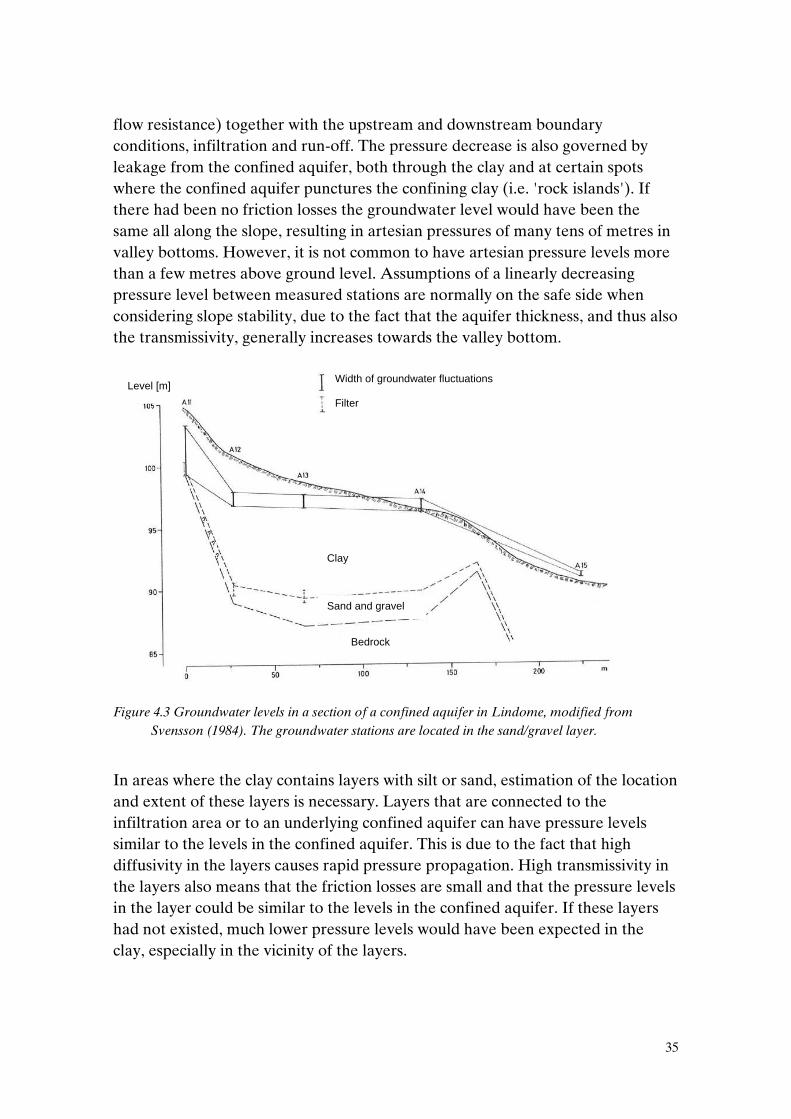
flow resistance) together with the upstream and downstream boundary conditions, infiltration and run-off. The pressure decrease is also governed by leakage from the confined aquifer, both through the clay and at certain spots where the confined aquifer punctures the confining clay (i.e. 'rock islands'). If there had been no friction losses the groundwater level would have been the same all along the slope, resulting in artesian pressures of many tens of metres in valley bottoms. However, it is not common to have artesian pressure levels more than a few metres above ground level. Assumptions of a linearly decreasing pressure level between measured stations are normally on the safe side when considering slope stability, due to the fact that the aquifer thickness, and thus also the transmissivity, generally increases towards the valley bottom.

Figure 4.3 Groundwater levels in a section of a confined aquifer in Lindome, modified from

Svensson (1984). The groundwater stations are located in the sand/gravel layer.

In areas where the clay contains layers with silt or sand, estimation of the location and extent of these layers is necessary. Layers that are connected to the infiltration area or to an underlying confined aquifer can have pressure levels similar to the levels in the confined aquifer. This is due to the fact that high diffusivity in the layers causes rapid pressure propagation. High transmissivity in the layers also means that the friction losses are small and that the pressure levels in the layer could be similar to the levels in the confined aquifer. If these layers had not existed, much lower pressure levels would have been expected in the clay, especially in the vicinity of the layers.

Clay

Bedrock

Sand and gravel

Width of groundwater fluctuations Filter

Level [m]

36

The extension of the sand/silt layer towards the valley middle, and possibly towards the slope face, is also important. In cases where a layer disappears in the middle of the clay, the flow though the layer is limited by the low hydraulic conductivity of the clay, causing small friction losses along the layer. When a layer has a downstream connection e.g. to an aquifer or by forming a well in the slope face, the flow and the friction losses will be higher. Consequently, sand/silt layers that disappear inside the clay represent a greater risk of high pore pressures developing than layers with a downstream connection.

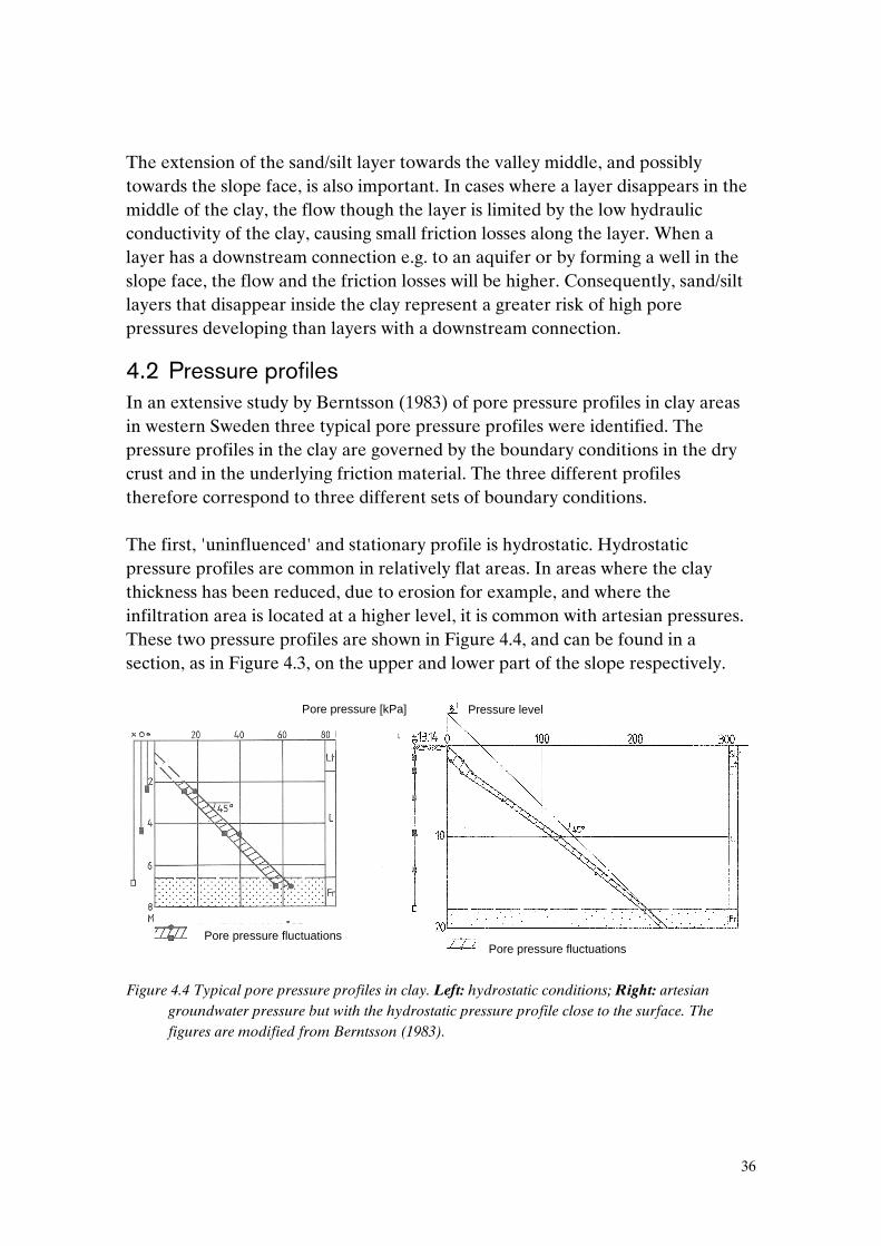
4.2 Pressure profiles In an extensive study by Berntsson (1983) of pore pressure profiles in clay areas in western Sweden three typical pore pressure profiles were identified. The pressure profiles in the clay are governed by the boundary conditions in the dry crust and in the underlying friction material. The three different profiles therefore correspond to three different sets of boundary conditions. The first, 'uninfluenced' and stationary profile is hydrostatic. Hydrostatic pressure profiles are common in relatively flat areas. In areas where the clay thickness has been reduced, due to erosion for example, and where the infiltration area is located at a higher level, it is common with artesian pressures. These two pressure profiles are shown in Figure 4.4, and can be found in a section, as in Figure 4.3, on the upper and lower part of the slope respectively.

Figure 4.4 Typical pore pressure profiles in clay. Left: hydrostatic conditions; Right: artesian

groundwater pressure but with the hydrostatic pressure profile close to the surface. The figures are modified from Berntsson (1983).

Pressure level

Pore pressure fluctuations Pore pressure fluctuations

Pore pressure [kPa]

37

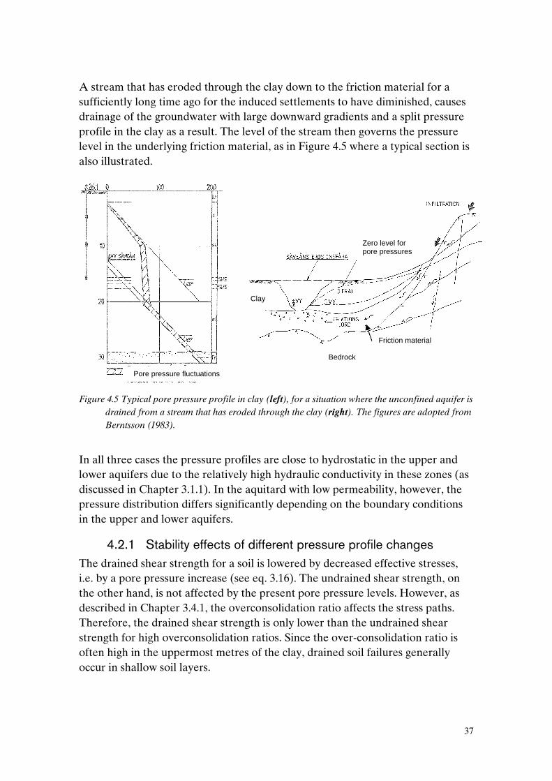
A stream that has eroded through the clay down to the friction material for a sufficiently long time ago for the induced settlements to have diminished, causes drainage of the groundwater with large downward gradients and a split pressure profile in the clay as a result. The level of the stream then governs the pressure level in the underlying friction material, as in Figure 4.5 where a typical section is also illustrated.

Figure 4.5 Typical pore pressure profile in clay (left), for a situation where the unconfined aquifer is

drained from a stream that has eroded through the clay (right). The figures are adopted from Berntsson (1983).

In all three cases the pressure profiles are close to hydrostatic in the upper and lower aquifers due to the relatively high hydraulic conductivity in these zones (as discussed in Chapter 3.1.1). In the aquitard with low permeability, however, the pressure distribution differs significantly depending on the boundary conditions in the upper and lower aquifers.

4.2.1 Stability effects of different pressure profile changes The drained shear strength for a soil is lowered by decreased effective stresses, i.e. by a pore pressure increase (see eq. 3.16). The undrained shear strength, on the other hand, is not affected by the present pore pressure levels. However, as described in Chapter 3.4.1, the overconsolidation ratio affects the stress paths. Therefore, the drained shear strength is only lower than the undrained shear strength for high overconsolidation ratios. Since the over-consolidation ratio is often high in the uppermost metres of the clay, drained soil failures generally occur in shallow soil layers.

Pore pressure fluctuations

Friction material

Bedrock

Zero level for pore pressures

Clay

38

A principal situation is presented in Figure 4.6 below, of a profile with a thick confining clay layer, and where pressure level changes occur only in the dry crust or in the confined aquifer at a time. As seen from the figure, pressure level changes in a confined aquifer only affect the pore pressure in shallow clay layers to a small extent. Consequently, high pressure in a confined aquifer is mainly a problem in areas with moderate clay depths and in areas with high permeable layers within the clay. For the shallow clay layers, pressure changes in the dry crust can have a much greater influence. However, the pore pressure effects from pressure level changes in the dry crust normally are smaller than the effects from the confined aquifer. In areas with a thick dry crust, severely raised pressure levels in the upper aquifer can though have considerably effect on the pore pressures in shallow potential slip surfaces.

dry crust

friction material

clay

pressure level

hydrostatic pressure

pressure change in friction material

pressure change in dry crust

level with equal pressure changes

Figure 4.6 Pore pressure level distributions, from variations in the dry crust or in the friction

material. The pressure level changes are not meant to illustrate typical pressure level changes, but merely a principal situation.

4.3 Pressure fluctuation Groundwater levels and pore pressures fluctuate over time, with large geographical differences due to climate variations, as illustrated in Figure 4.7. In northern Sweden the groundwater levels have a distinct maximum level in late spring, due to snow melt, while in middle/southern Sweden a secondary maximum during autumn and winter can also be seen.

39

Figure 4.7 Typical yearly groundwater level variations in different regions of Sweden, from

Thunholm (2008).

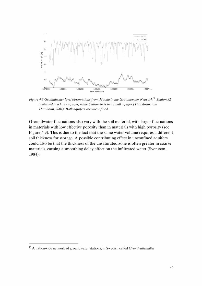
The fluctuations also depend on the aquifer size, as can be seen in Figure 4.8. In large groundwater reservoirs the groundwater levels can increase or decrease over a period of several years and dominate over seasonal and short-term variations. In small reservoirs, the variation between different years is much smaller than the seasonal fluctuations and the fluctuation amplitude is also greater than in large reservoirs (Thorsbrink and Thunholm, 2004).

40

1974-06 1980-01 1985-08 1991-02 1996-09 2002-04 2007-11-6

-5

-4

-3

-2

-1

0

1

Leve

l rel

. to

g.l.

[m

]

Year and month

no. 32

no. 46

Figure 4.8 Groundwater level observations from Motala in the Groundwater Network13. Station 32

is situated in a large aquifer, while Station 46 is in a small aquifer (Thorsbrink and Thunholm, 2004). Both aquifers are unconfined.

Groundwater fluctuations also vary with the soil material, with larger fluctuations in materials with low effective porosity than in materials with high porosity (see Figure 4.9). This is due to the fact that the same water volume requires a different soil thickness for storage. A possible contributing effect in unconfined aquifers could also be that the thickness of the unsaturated zone is often greater in coarse materials, causing a smoothing delay effect on the infiltrated water (Svensson, 1984).

13 A nationwide network of groundwater stations, in Swedish called Grundvattennätet

41

Figure 4.9 Groundwater level fluctuations in soil materials with different effective porosity,

measured at the Groundwater Network area in Tärnsjö. Figure adopted from Svensson (1984), who adopted it from Knutsson and Fagerlind (1977). [Granit, morän, sand and gravel (in Swedish) are granit, till, sand and gravel respectively.]

The response in the groundwater level due to a specific level of rainfall differs significantly in different aquifers, with a much quicker response in confined rather than in unconfined aquifers. In addition, groundwater level fluctuations show different patterns also between confined aquifers in the same area (see Figure 4.10). The yearly fluctuations among the stations studied are in the range 1-3 m. In confined aquifers the fluctuation amplitude is generally largest close to the infiltration areas and decreases towards the middle of the aquifer. The reason for this fluctuation decreases are dampening effects from the aquifer's diffusivity and to averaging effects from infiltration from different directions. Moreover, and perhaps more important, is the downstream boundary condition that for example can be governed by the sea level and therefore be quite constant. A constant downstream condition thus causes smaller fluctuation amplitudes in the downstream parts of an aquifer.

42

Figure 4.10 Groundwater level variations in confined aquifers in Sandsjöbacka. Station 5213 has a

larger response to the precipitation events in late November than the other stations. Figure adopted from Svensson (1984).

Groundwater level responses observed at the stations in the slope in Figure 4.3, are illustrated in Figure 4.11. The response delay between A11 and A12 was in the order of 7-16 hours. Between A12 and A14 no delay was observed and between A14 and A15 the delay was estimated at 8-16 hours (Svensson, 1984). In an aquifer with high diffusivity the response delay can, however, be very small. According to Svensson (1984) this was the case for the distance between A12 and A14. A similar situation was observed in the Småröd landslide investigation, where the fluctuation patterns were almost identical in two pore pressure gauges, located 150 m apart and covered by 20 and 33 m of clay respectively (see Figure 4.11).

Figure 4.11 Left: observed groundwater level fluctuations from the slope illustrated in Figure 4.3.

Adopted from Svensson (1984). Right: pore pressure fluctuations in the friction material at two locations, 150 m apart, in the Småröd landslide. Adopted from Hartlén et al. (2007).

43

4.3.1 Non-infiltration causes of fluctuation The main cause of groundwater pressure fluctuations is, as mentioned earlier, climatological effects such as precipitation and evaporation. However, pressure changes can also be caused by loading effects, both from atmospheric pressure and external loading. The atmospheric pressure effects are discussed to some extent in the groundwater level measurement section in Chapter 8.2. External loading can be caused by construction work, vehicles etc., but also by precipitation accumulated in the dry crust. In contrast to increased groundwater levels, external loading increases the total stress. Bockgård (2004) suggests that the pressure fluctuations in large confined aquifers are caused by seasonal storage changes in the overlying clay and not by storage changes in the aquifer. Since most of the clay is always water-saturated, this storage must occur in the dry crust. Although this issue has not been investigated further, a preliminary estimation is that the amount of water that can be accumulated in the dry crust is generally quite small. Consequently, the direct effect of increased storage in the uppermost soil layers should be quite small in the groundwater levels in an underlying confined aquifer.

5 MODELLING AND PREDICTION OF GROUNDWATER LEVELS

Modelling and prediction of groundwater levels is done within different academic disciplines and for different purposes, e.g. for water resource planning, improvement of run-off calculations and in geotechnical engineering for settlement and slope stability calculations (e.g. Bergström and Sandberg, 1983; Svensson, 1984; Seibert et al., 1997; Colleuille et al., 2006; Ramli et al., 2007). Common to all models is that they are a representation of reality and are based on certain assumptions. The methodology and the scale of the model can, however, vary considerably, from general hydrological models on a catchment scale to detailed hydrogeological models of a specific slope. In addition, there are statistical models that are not easily associated with a specific scale. Models can also have different levels of simplification and approaches for describing a certain phenomenon. Physical models aim to take all physical processes involved into account; conceptual models aim to describe results but can have highly simplified descriptions of the actual processes involved. The input parameters can also vary in different models even though the output quantity is the same.

44

This chapter focuses on modelling and prediction of groundwater levels in confined aquifers with an emphasis on the maximum levels. Most of the modelling has been done using a slightly modified version of the hydrological HBV14 model since it is a simple and commonly used model. As a complement, a detailed model using the FEM (finite element method) program SEEP has been briefly tested. It is also suggested that a 'middle way method' could be appropriate for future modelling, where the most important parts of the geological profile are identified and described in detail, while other parts are simplified substantially.

5.1 The HBV model The HBV model is a well-established conceptual rainfall-runoff model, developed by Bergström (1976). The model has been used in more than 40 countries (SMHI, 2008). It was originally developed for run-off simulations and hydrological forecasting, but has since then been used for an increasing number of different applications, e.g. for nutrient transport by Lindström et al. (2005) and prediction of groundwater levels by Lindström et al. (2002). The HBV model has also been used for investigations into the influence of climate change on run-off and soil moisture (e.g. Andréasson et al., 2004). The HBV model was developed for areas dominated by unconfined aquifers and most model applications over the years have accordingly been for unconfined aquifers. However, some studies have simulated groundwater level fluctuations in confined aquifers (e.g. Sandberg, 1982; Bergström and Sandberg, 1983; Rosén, 1991; Johnson, 1993). When applying the model to areas with confined aquifers, the model is a highly conceptual representation of reality and does not describe the actual physical processes. Accordingly, great care must be taken when interpreting and extrapolating the model results. The HBV model is a water balance model, the main input parameters being precipitation and temperature. Additional input items are, for example, estimates of potential evapotranspiration, and to some extent also topography and type of vegetation. The general principle of the model is that precipitation and snowmelt infiltrate the soil and increase the soil moisture, from which water either evaporates or causes recharge into the groundwater zone. The groundwater zone is divided into two separate reservoirs, upper and lower, which are the origins of the quick and slow responses to run-off respectively. Output from the model is

14 The name HBV was originally an abbreviation for a division at SMHI called Hydrologiska Byråns Vattenbalansavdelning (Hydrology Office, Water Balance Department).

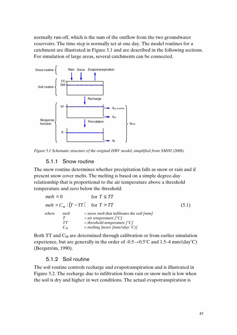
45

normally run-off, which is the sum of the outflow from the two groundwater reservoirs. The time step is normally set at one day. The model routines for a catchment are illustrated in Figure 5.1 and are described in the following sections. For simulation of large areas, several catchments can be connected.

Rain Snow Evapotranspiration

Recharge

Percolation

FC SM

lz

uz quz,overf low

quz

qlz

qtotal

Snow routine

Soil routine

Response function

Figure 5.1 Schematic structure of the original HBV model, simplified from SMHI (2008).

5.1.1 Snow routine The snow routine determines whether precipitation falls as snow or rain and if present snow cover melts. The melting is based on a simple degree-day relationship that is proportional to the air temperature above a threshold temperature and zero below the threshold.

0=melt for TTT ≤

( )TTTCmelt M −⋅= for TTT > (5.1)

where melt = snow melt that infiltrates the soil [mm] T = air temperature [°C] TT = threshold temperature [˚C] CM = melting factor [mm/(day·˚C)]

Both TT and CM are determined through calibration or from earlier simulation experience, but are generally in the order of -0.5–+0.5˚C and 1.5–4 mm/(day˚C) (Bergström, 1990).

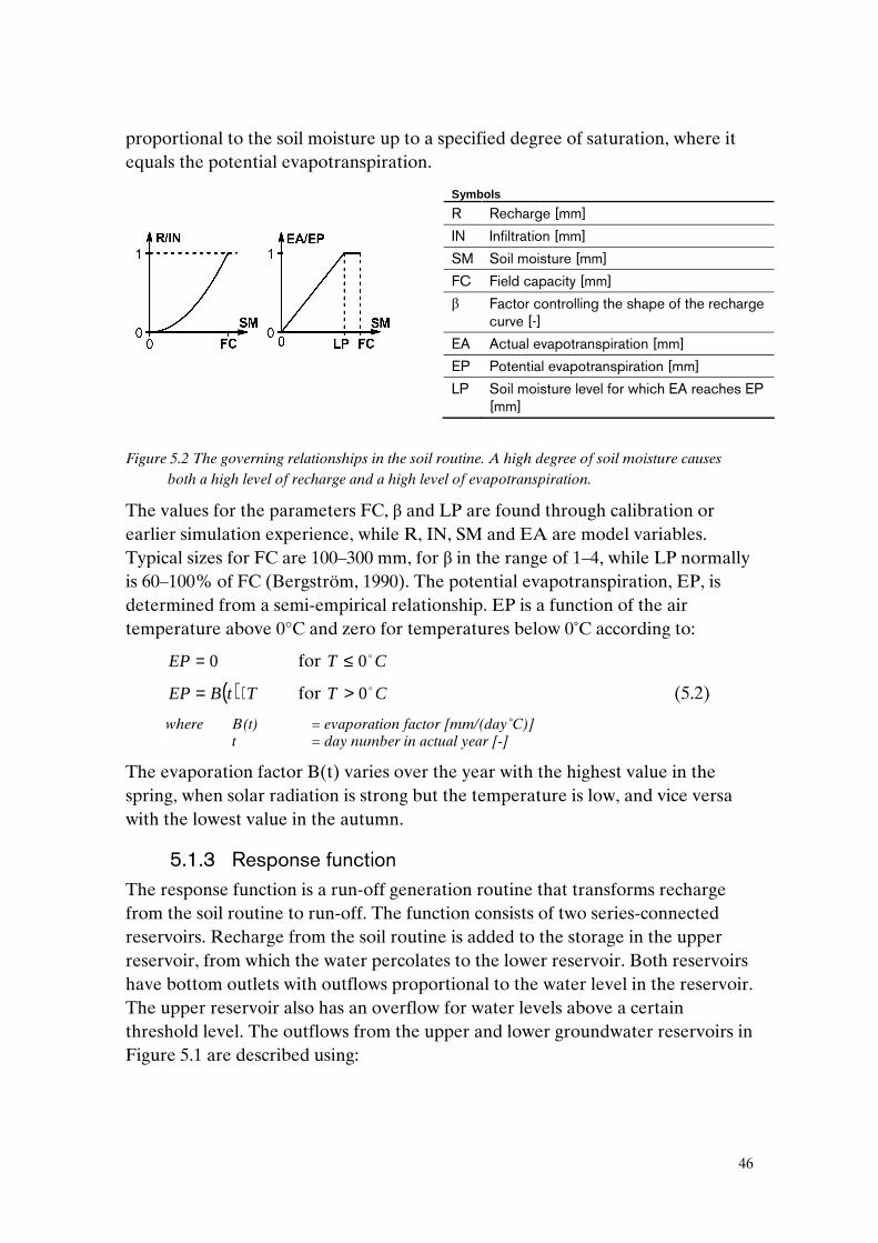
5.1.2 Soil routine The soil routine controls recharge and evapotranspiration and is illustrated in Figure 5.2. The recharge due to infiltration from rain or snow melt is low when the soil is dry and higher in wet conditions. The actual evapotranspiration is

46

proportional to the soil moisture up to a specified degree of saturation, where it equals the potential evapotranspiration.

Figure 5.2 The governing relationships in the soil routine. A high degree of soil moisture causes

both a high level of recharge and a high level of evapotranspiration.

The values for the parameters FC, β and LP are found through calibration or earlier simulation experience, while R, IN, SM and EA are model variables. Typical sizes for FC are 100–300 mm, for β in the range of 1–4, while LP normally is 60–100% of FC (Bergström, 1990). The potential evapotranspiration, EP, is determined from a semi-empirical relationship. EP is a function of the air temperature above 0°C and zero for temperatures below 0˚C according to:

0=EP for CT o0≤

( ) TtBEP ⋅= for CT o0> (5.2)

where B(t) = evaporation factor [mm/(day˚C)] t = day number in actual year [-]

The evaporation factor B(t) varies over the year with the highest value in the spring, when solar radiation is strong but the temperature is low, and vice versa with the lowest value in the autumn.

5.1.3 Response function The response function is a run-off generation routine that transforms recharge from the soil routine to run-off. The function consists of two series-connected reservoirs. Recharge from the soil routine is added to the storage in the upper reservoir, from which the water percolates to the lower reservoir. Both reservoirs have bottom outlets with outflows proportional to the water level in the reservoir. The upper reservoir also has an overflow for water levels above a certain threshold level. The outflows from the upper and lower groundwater reservoirs in Figure 5.1 are described using:

Symbols

R Recharge [mm]

IN Infiltration [mm]

SM Soil moisture [mm]

FC Field capacity [mm]

β Factor controlling the shape of the recharge curve [-]

EA Actual evapotranspiration [mm]

EP Potential evapotranspiration [mm]

LP Soil moisture level for which EA reaches EP [mm]

47

uzkq uzuz ⋅= (5.3)

( )overflowuzoverflowuzoverflowuz luzkq ,,, −⋅= (5.4)

lzkq lzlz ⋅= (5.5)

where quz = bottom outflow from the upper groundwater reservoir [mm/day] quz,overflow = overflow outflow from the upper groundwater reservoir [mm/day] qlz = bottom outflow from the lower groundwater reservoir [mm/day] uz = level in the upper groundwater reservoir [mm]15 lz = level in the lower groundwater reservoir [mm] luz,overflow = overflow level in uz [mm] kuz = proportionally constant for the bottom outflow from uz [1/day]

kuz,overflow = proportionally constant for the overflow from uz [1/day] klz = proportionally constant for the bottom outflow from lz [1/day]

The proportionally constants kuz, kuz,overflow and klz are, together with luz,overflow, determined from calibration, while uz, lz, quz, qlz and qlz,overflow are model variables. For one single recharge occurrence, the percolation from uz to lz is greatest on the first day and then decreases with time. For example, a value of kuz = 0.5 1/day means that 50% of the recharged water will reach the lower groundwater reservoir within one day. The following day 50% of the remaining water will reach it, meaning that 75% of the infiltrated precipitation reaches the lower reservoir within two days. With kuz = 0.1 1/day, it takes 13 days for 75% of the recharged water to reach the lower reservoir. Figure 5.3 illustrates the interaction between the upper and the lower groundwater reservoirs for one single recharge occurrence.

0

0.2

0.4

0.6

0.8

1

1.2

0 10 20 30 40 50

days

leve

l [m

m] uz

lz

Accumulated qlz

Figure 5.3 Response in the upper and lower groundwater reservoirs, uz and lz, to a single 1 mm

recharge to uz. The response routine parameters are: kuz = kuz = 0.1 1/day and no overflow occurs from uz. The accumulated outflow from lz is also shown.

15 uz and lz are also used to denote the upper and lower groundwater reservoirs respectively.

48

5.1.4 The Harestad model An attempt to simulate the groundwater levels in confined aquifers using a modified HBV model was made by Bergström and Sandberg (1983) in the Harestad area north of Gothenburg. A description of the Harestad area is presented in Chapter 7. Bergström and Sandberg used a model set-up almost identical to the original HBV model in Figure 5.1. The authors' idea was to describe the fluctuations in the deep parts of the confined aquifer using the lower reservoir and with the upper reservoir representing the shallow parts. The overflow level in the upper reservoir was meant to represent surface drainage from the bare rock areas, which reduces the amount of water that percolates to the confined aquifer. Bergström and Sandberg stress that the transition from the upper to the lower reservoir is the main problem when simulating confined aquifers. The authors also point out that their initial assumption that groundwater fluctuations in the upper part of the confined aquifer, i.e. close to the infiltration areas, would be best described using the upper reservoir had to be rejected. The fluctuations at all groundwater stations were thus described using the lower reservoir. A model set-up, complemented with an overflow in the lower reservoir, was also tested and it showed promising results. Furthermore, it was pointed out that it is difficult to determine whether the daily variations in the simulations are correct, since the groundwater level measurements available for calibration were registered every 14 days. Bergström and Sandberg (1983) also noted that some of the model parameters did not have an obvious physical interpretation and could not be compared directly with any known quantity.

5.2 SEEP SEEP is a commercial two-dimensional groundwater modelling tool developed by GEO-SLOPE (2008), using FEM (finite element method). Since SEEP is integrated with the slope stability program SLOPE, it is popular among geotechnical engineers. The program is based on the groundwater flow equation, described in equation 3.12. The program is capable of handling both saturated and unsaturated situations as well as steady state and transient conditions. For saturated, steady-state analyses, soil hydraulic conductivity must be specified and for transient analyses soil stiffness is also required. When unsaturated conditions appear in the model a water content curve (for negative water pressures) must also be specified.

49

5.3 The Chalmers model The Chalmers model, developed by Svensson (1984), is a statistical model for calculating the maximum groundwater levels expected at a specific site within a certain design period. The model is recommended in Sweden for predictions of maximum pore pressures in slope stability calculations (CoSS, 1995). However, it is not commonly used and, as mentioned in Chapter 1, other methods dominate. The model is based on correlation of groundwater fluctuations in geologically and climatologically similar aquifers. Groundwater level measurements from a short observation period at a previously unmeasured site are compared with a series of groundwater observations from a nearby reference area where extensive records of groundwater levels are available. Svensson (1984) also found that the topographical position within the aquifer is important since the groundwater level generally fluctuates more in areas close to infiltration areas. The groundwater level with a certain return period in the reference area is calculated by assuming that the maximum groundwater levels from every hydrological year16 are normally distributed. An estimate of the maximum groundwater level, with a 200-year return period, in a prediction area is calculated from equation 5.6 and is illustrated in Figure 5.4 (Svensson, 1984).

R

PR r

rSPP ⋅+= 200

max200

max (5.6)

where 200maxP = maximum level in the prediction station with a return period of

200 years Pmax = maximum level in the prediction station during the observation

period

200RS = | 200

maxy -ymax|

200maxy = maximum level for the reference station with a return period of

200 years ymax = maximum level for the reference station during the observation

period rP = variation in the groundwater level in the prediction station during

the observation period rR = variation in the groundwater level in the reference station during the

observation period

16 Is defined as October 1 – September 30

50

Figure 5.4 Usage of the Chalmers model for estimation of maximum and minimum groundwater

levels with a return period of 200 years, modified from (Svensson and Sällfors, 1985). The calculated maximum and minimum levels have been illustrated as a function varying over the year, even though the model output is normally only one single level. [Grundvattennivå (in Swedish) means groundwater level.]

The model was originally developed for prediction of groundwater levels in confined aquifers. However, Berntsson (1983) showed that the pore pressures in clay have variations proportional to the variations in confined aquifers. Therefore the model is also recommended for use in predicting maximum pore pressures in clay (CoSS, 1995). High correlation of the fluctuations in different aquifers can only be expected in relatively small aquifers, where the variations between different years are smaller than the variations within a particular year. Consequently, the model is only applicable for small aquifers. Svensson (1984) recommends that the correlation coefficient of the fluctuations at the reference and the prediction stations is at least 0.9. Svensson also found that the pressure variation at the reference station within the prediction period should be at least 30% of the total variation at the station. He also recommends that the fluctuation amplitude at the reference station is larger than at the prediction station. In addition, Svensson recommends that the observations at the prediction station should be made for a period of at least three months to obtain good prediction results. The effect of different prediction period lengths is illustrated in Figure 5.5, where predictions of maximum levels have been made using several reference stations.

Reference station Prediction station

51

Bengtsson and Boström (2008) argue that a spread of the predicted maximum levels of less than one metre can be considered a good result. A mean value of the predicted levels is suggested to be a good estimation of the maximum levels, which can be further improved by assigning greater weight to predictions from reference stations located in similar aquifer positions.

Number of observations (with a 14-day interval)6 8 10 12 14 16-100

-80

-60

-40

-20

0

20

40

Level [cm]Successiv förlängning av pro gnostid med flera referensrör.

Prognosrör 52008Startdatum 1992-06-15

52002520045200952011520135201469003'Real max'

Figure 5.5 Prediction, using the Chalmers model, of the maximum level with a 200-year return

period for Station 5208. To improve the prediction, several reference stations have been used. The 'real' level, with a 200-year return period, has been calculated from the data series for 5208. Figure modified from Bengtsson and Boström (2008).

Bengtsson and Boström (2008) made a large number of groundwater level predictions within the Sandsjöbacka area and compared the predicted levels with the 'real' levels. The predictions were carried out for levels with a 200-year return period, and the 'real' levels were determined from statistical analyses of long-term observations from the prediction stations. The prediction results, shown in Figure 5.6, indicate a relatively good level of precision and small errors for most of the predictions.

52

Figure 5.6 Histogram showing the absolute value of groundwater level predictions, using the

Chalmers model, carried out within the Sandsjöbacka area. Figure modified from Bengtsson & Boström (2008).

5.3.1 Model strengths and areas of improvement One of the most obvious strengths of the Chalmers model is that a short groundwater level series in a prediction station is complemented with groundwater fluctuation information from long observation series in similar reference stations. Furthermore, the required knowledge of the local hydrogeology is low, which means that the cost of the predictions is low. When used properly, the model also seems to produce good results. However, the underlying assumptions in the Chalmers model raise several questions. A central issue is the correlation of fluctuation patterns at the reference and prediction stations, which brings to the fore the problem of the relatively sparse Groundwater Network. The Chalmers method cannot be used with good results when the distance between the reference and prediction stations is too large, since the groundwater fluctuation patterns might have unacceptable differences. One way of handling problems arising from the sparsity of available reference stations could be to simulate reference station fluctuations, or possibly to simulate the prediction station fluctuations directly. This type of groundwater level modelling is tested in a few case studies in Chapter 9. The importance of having a reference and prediction station in similar aquifers and positions must therefore be weighed up against the effects of having a more

0 10 20 30 40 50 60 70 100 150 200

0

100

200

300

400

500

600

700

800

900

1000

Prediction error [cm] 0 50 150

53

distant reference area. The effect of aquifer position on fluctuation patterns is discussed briefly in Chapter 4.3, and also in the case study Chapters 8 and 9. Another important issue is the functionality of the reference groundwater stations. Studies of the fluctuation patterns of the Groundwater Network have in several cases indicated malfunctioning of the stations and simple field tests have revealed problems with several reference stations. The functionality of the Groundwater Network is further discussed in Chapter 8. Bengtsson and Boström (2008) recommend that the reference and prediction stations should have time-lags in the same order of magnitude. The effect of overflowing aquifers is included to some extent in the Chalmers model. However, if a reference station with a distinct overflow is used for predicting the levels in an aquifer without an overflow level, the results could be highly misleading. This is also true of the opposite situation, with an overflow in the prediction aquifer but not at the reference station.

5.3.2 Maximum pressure levels Svensson (1984) studied the distribution of the yearly maximum groundwater levels in the Groundwater Network, and suggested that they are normally distributed. This suggestion can be questioned, as shown in the Pearson diagram in Figure 5.7, even though the correspondence between the observations and the suggested normal distribution was improved substantially with the removal of certain erroneous observations. In a Pearson diagram, the skewness for the data series is plotted on the x-axis and the kurtosis on the y-axis. A normally distributed data series, with zero skewness and a kurtosis of three, is thus located at the co-ordinate (0,3).

54

Figure 5.7 Pearson diagrams from Svensson (1984), where the left graph is modified from Pearson

and Hartley (1972) and β1 stands for skewness and β2 for kurtosis. Left: graph indicating where different distributions can be found; Right: analyses of the yearly maximum values, where the arrows and circles indicate where the data series is located when erroneous observations are removed from the data series.

These findings were confirmed by Alén (1998) and Bengtsson and Boström (2008), who point out that the assumption of a normal distribution is only valid for some stations. Furthermore, the yearly maximum levels for most of the analysed groundwater stations have a negatively skewed distribution and are thus restrained upwards. This is suggested as having the physical explanation that there are overflows in the aquifers (Alén, 1998). Bengtsson and Boström also concluded that the stations without negative skewness were malfunctioning. An assumption of normally distributed maximum levels leads to an overestimation of the maximum levels if the true distribution has a negative skewness. For the stations in the Gothenburg area, the largest level difference for a 200-year return period prediction, between an assumed normal distribution and a general extreme value distribution was found to be 16 cm (Bengtsson and Boström, 2008). Alén (1998) found that in certain cases a distinct threshold level was present in the yearly maximum level series. A reasonable approach according to Alén is to describe the levels below and above this threshold with different distributions. The threshold level can be found from a probability plot as in Figure 5.8. To take

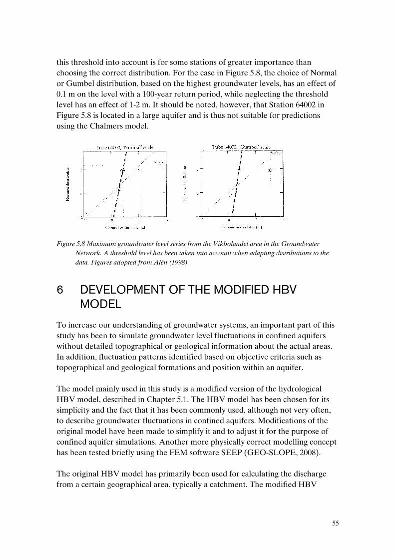
55

this threshold into account is for some stations of greater importance than choosing the correct distribution. For the case in Figure 5.8, the choice of Normal or Gumbel distribution, based on the highest groundwater levels, has an effect of 0.1 m on the level with a 100-year return period, while neglecting the threshold level has an effect of 1-2 m. It should be noted, however, that Station 64002 in Figure 5.8 is located in a large aquifer and is thus not suitable for predictions using the Chalmers model.

Figure 5.8 Maximum groundwater level series from the Vikbolandet area in the Groundwater

Network. A threshold level has been taken into account when adapting distributions to the data. Figures adopted from Alén (1998).

6 DEVELOPMENT OF THE MODIFIED HBV MODEL

To increase our understanding of groundwater systems, an important part of this study has been to simulate groundwater level fluctuations in confined aquifers without detailed topographical or geological information about the actual areas. In addition, fluctuation patterns identified based on objective criteria such as topographical and geological formations and position within an aquifer. The model mainly used in this study is a modified version of the hydrological HBV model, described in Chapter 5.1. The HBV model has been chosen for its simplicity and the fact that it has been commonly used, although not very often, to describe groundwater fluctuations in confined aquifers. Modifications of the original model have been made to simplify it and to adjust it for the purpose of confined aquifer simulations. Another more physically correct modelling concept has been tested briefly using the FEM software SEEP (GEO-SLOPE, 2008). The original HBV model has primarily been used for calculating the discharge from a certain geographical area, typically a catchment. The modified HBV

56

model in this study is used for calculating the groundwater levels in a confined aquifer at a certain geographical point and thus has no areal representation. As described in Chapter 3.1, the infiltration and recharge through clay soils is very low. Accordingly, the recharge into confined aquifers occurs to a large extent along the clay boundaries in more permeable soils or fractured rock. The absence of vertical recharge means that a pressure increase in an aquifer is created by mainly horizontal pressure propagation rather than by vertical groundwater seepage. In the modified HBV model, the groundwater recharge into a confined aquifer is treated in the same way as recharge into an unconfined aquifer, meaning that the model description is highly conceptual. The interpretation of the modified HBV model in a confined aquifer is illustrated in Figure 6.1.

Rain Snow Evapotranspiration

FC SM

lz qlz,overf low

qlz

Clay

Groundwater station

uz

quz

’Percolation’

Recharge

Figure 6.1 Schematic structure of the modified HBV model and the interpretation of its use in a

confined aquifer. The overflow level in the lower groundwater reservoir is llz,overflow.

6.1 Model structure The model structure is a stripped and modified one catchment version of the original HBV model. The main difference compared to the original model is that there are no water outlets from the upper groundwater reservoir other than the percolation. On the other hand, there is an overflow in the lower groundwater reservoir as indicated in Figure 6.1. Moreover, the original soil routine has been replaced with a soil routine, as shown in Figure 6.2, according to Rodhe et al.(2006). In the snow routine, the threshold temperature, described in equation 5.1, is set at 0°C.

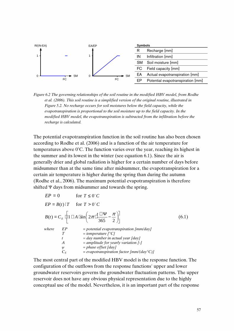
57

Figure 6.2 The governing relationships of the soil routine in the modified HBV model, from Rodhe

et al. (2006). This soil routine is a simplified version of the original routine, illustrated in Figure 5.2. No recharge occurs for soil moistures below the field capacity, while the evapotranspiration is proportional to the soil moisture up to the field capacity. In the modified HBV model, the evapotranspiration is subtracted from the infiltration before the recharge is calculated.

The potential evapotranspiration function in the soil routine has also been chosen according to Rodhe et al. (2006) and is a function of the air temperature for temperatures above 0˚C. The function varies over the year, reaching its highest in the summer and its lowest in the winter (see equation 6.1). Since the air is generally drier and global radiation is higher for a certain number of days before midsummer than at the same time after midsummer, the evapotranspiration for a certain air temperature is higher during the spring than during the autumn (Rodhe et al., 2006). The maximum potential evapotranspiration is therefore shifted Ψ days from midsummer and towards the spring.

0=EP for CT o0≤

TtBEP ⋅= )( for CT o0>

−Ψ+⋅⋅+⋅=2365

2sin1)(ππ t

ACtB E (6.1)

where EP = potential evapotranspiration [mm/day] T = temperature [°C] t = day number in actual year [day] A = amplitude for yearly variation [-] ψ = phase offset [day] CE = evapotranspiration factor [mm/(day°C)]

The most central part of the modified HBV model is the response function. The configuration of the outflows from the response functions' upper and lower groundwater reservoirs governs the groundwater fluctuation patterns. The upper reservoir does not have any obvious physical representation due to the highly conceptual use of the model. Nevertheless, it is an important part of the response

R/(IN-EA)

1

0 SM FC

EA/EP

1

0 SM FC

Symbols

R Recharge [mm]

IN Infiltration [mm]

SM Soil moisture [mm]

FC Field capacity [mm]

EA Actual evapotranspiration [mm]

EP Potential evapotranspiration [mm]

58

function and can be comprehended as a smoothening delay for the groundwater level response to precipitation. The delay in the upper reservoir is related to the position within the aquifer and to the aquifer diffusivity. The lower groundwater reservoir represents the groundwater storage above the lowest possible groundwater level and the overflow in the lower reservoir represents the over-all aquifer overflow. In the Harestad model, presented in Chapter 5.1.4, the overflow in the upper reservoir is intended to represent overflow through surface drainage, causing reduced infiltration. In the modified HBV model this phenomenon is included in the calibration parameters. The overflow in the lower reservoir, however, would appear to be crucial in describing the restrained maximum levels of the groundwater level fluctuations. The overflowing water is described using equation 6.2. The choice of quadratic dependence on the groundwater level is quite arbitrary17. A different choice of overflow function would mainly affect the value of the overflow constant.

( )2,,, overflowlzoverflowlzoverflowlz llzkq −⋅= (6.2)

where qlz,overflow = overflowing water [mm/day] klz,overflow = proportional constant [1/(mm·day)]18 lz = water level in the lower groundwater reservoir [mm] llz,overflow = threshold level for overflow [mm]

To describe groundwater levels, the level in the lower groundwater reservoir is transformed to a groundwater level by considering 'effective porosity'19 in the aquifer:

( )ep

lzzlzzgw ⋅⋅+=10

1min (6.3)

where zgw = groundwater level [cm rel. to g.l.] zmin = reference level (lowest possible/measured g.w. level) [cm rel. to g.l.] lz = groundwater storage in lower reservoir [mm] ep = 'effective porosity' [-]

6.2 Model parameters To keep the modified HBV model as simple as possible, and to be able to identify the parameters governing the groundwater fluctuation characteristics, the number of model parameters has been reduced in comparison to the original 17 Flow over a rectangular overflow is proportional to (the water level)3/2 and for a triangular

overflow to (the water level)5/2, meaning that the assumed overflow has a trapezoidal geometry. 18 Since the overflow has been assumed to be proportional to the square of the water level, the unit of the coefficient differs from the other flow coefficients in the model. 19 The term 'effective porosity' is used, although the effective porosity affects the fluctuations in the infiltration area rather than at the groundwater station.

59

HBV model. Furthermore, as many parameters as possible have been assigned fixed values for all simulations and these parameters are presented in Table 6-1. The total number of model parameters is 11, of which six have fixed values for all simulations and one is assigned a specific value for each station, meaning that four parameters are calibrated for each groundwater station. Rodhe et al. (2006) found that the field capacity for the soil types coarse, till and fine, in Sweden, is 70, 244 and 366 mm respectively. This indicates that fine soils have a high field capacity and clay should therefore have a field capacity of at least 366 mm. However, these values are based primarily on simulations of open aquifers and vertical infiltration through the soils. Since infiltration into confined aquifers only occurs along the clay edges, where the bedrock is bare or covered with thin soil layers, the water-holding capacity, and thus the field capacity in the infiltration area, is small. Consequently, the field capacity in the modified model should be relatively small. The size FC = 100 mm was chosen, rather arbitrarily. A different choice of field capacity would affect the size of the calibrated parameters. Since the clay along the Swedish west coast generally covers layers of till soils, effective porosity corresponding to till soil has been chosen for the transformation from a water level in the lower reservoir to a groundwater level in the aquifer. Furthermore, the lowest registered groundwater level was assumed to be the lowest possible level.

Table 6-1 The modified HBV model parameters with fixed values for all simulations. Parameter values from Rodhe et al. (2006).

Parameter Value Description

CM 2.5 Snow melting factor

CE 0.19 Evapotranspiration factor

A 0.5 Amplitude for yearly variation of potential evaporation

Ψ 45 Shift in maximal potential evaporation from mid-summer (i.e. to mid-May)

FC 100 Field capacity for the aquifer infiltration zone

ep 0.05 Effective porosity in the aquifer underlying the clay

Four parameters have been calibrated for each groundwater station and are shown in Table 6-2. These are the proportional constants for the bottom outflows from the upper and lower groundwater reservoirs and for the overflow in the lower reservoir, together with the level for the overflow. Furthermore, the lowest

60

possible groundwater level is included in the table even though no real calibration has been made for this parameter.

Table 6-2 The modified HBV model parameters calibrated for each station.

Parameter Description

kuz Proportionally constant for bottom outflow from the upper reservoir

klz Proportionally constant for bottom outflow from the lower reservoir

klz,overflow Proportionally constant for overflow from the lower reservoir

llz,overflow Overflow level for the lower groundwater reservoir

zmin1 Lowest registered groundwater level

1 The parameter zmin has not been calibrated but has a specific value for each groundwater station.

6.3 Physical interpretation of the model The modified HBV model describes recharge into a confined aquifer in the same way as into an unconfined aquifer. However, physical understanding of the model parameters is not easily comparable for simulations in confined and unconfined aquifers. Attempts at physical interpretation of the modified HBV model are discussed below and are illustrated in Figure 6.1. There is further discussion of the model interpretation in the case studies in Chapter 9.5 The soil routine for the modified HBV model describes the infiltration areas for a certain groundwater station. These infiltration areas can be considered as unconfined aquifers and the water recharge thus has a direct effect on the groundwater level fluctuations. In a confined aquifer, the fluctuations in the infiltration area cause pressure propagations spreading throughout the aquifer. However, in the modified HBV model this pressure propagation is described by percolation from the upper groundwater reservoir. Since each modified HBV model is set up to describe one single groundwater station, the delay in the upper reservoir corresponds to the real pressure propagation delay for that specific station. From the upper groundwater reservoir, the water percolates to the lower reservoir. In the modified HBV model, the soil porosity is taken into account at the lower groundwater reservoir when calculating the groundwater levels, while in reality the porosity affects the fluctuations in the infiltration area. This is also the case for the groundwater overflow. In reality, overflow occurs in the infiltration areas while in the modified HBV model it occurs at a certain level in the lower groundwater reservoir.

61

The response function in the modified HBV model is thus a highly conceptual representation of the real pressure propagation in a confined aquifer. A more physical description of the pressure propagation, using the groundwater flow equation (equation 3.12), could simplify identification of the fluctuation-governing model parameters. The infiltration area can be regarded as an unconfined aquifer with low porosity, causing large groundwater level fluctuations. From the bottom of the infiltration area, a thin confined aquifer spreads out into the valley. At some spots the confining layer is broken by bedrock 'islands' reaching up through the clay. These places thus function as overflows but are too small for the precipitation to make any substantial contribution to the inflow. This more physical correct, but still conceptual, model for a confined aquifer could be illustrated as in Figure 6.3.

Infiltration area (unconfined aquifer)

Confined aquifer

Rain Snow Evapotranspiration

Clay

Possible overflow

Fixed groundwater level

Ground-water level fluctuation

Outflow

Possible overflow

Figure 6.3 A conceptual model of a typical confined aquifer with a more physical correct

description than in the modified HBV model.

A simple parameter study has been done for the confined aquifer part of Figure 6.3, but without overflows. A principal fluctuation pattern for the groundwater levels close to infiltration areas, with a distinct overflow level at the 11m level, has been set as a boundary condition on the model upstream side. The boundary on the downstream side is a variable water flow. The pressure propagation throughout the aquifer depends on the aquifers' diffusivity, while the pressure levels on the other hand depend on the aquifer transmissivity and the water flow through the aquifer. The pressure propagation through the aquifer, for three different sets of parameters, is presented in Figure 6.4. The fluctuation patterns differ significantly in the three cases, due to a wide span of parameter values. The knowledge of these parameter values is, however, limited, as well as the means for testing them, resulting in a high degree of uncertainty regarding the parameter values. For that reason, a parameter value uncertainty of a factor of 102, as in Figure 6.4, is quite realistic. More in-depth studies using the model in

62

Figure 6.3 could improve our knowledge of the size of these parameter values, but has not been done in this study.

Figure 6.4 Propagation of pressure level fluctuations at the distances 0, 77, 205, 289, 391 and 500 m

(measured from the upstream boundary) in a confined aquifer with a thickness, linearly increasing

from 0.1 m to 1 m over the length of 500 m. The three figures show results from different

parameter set-ups, with variations in hydraulic conductivity and outflow at the downstream

boundary. The oedometer modulus is equal to M=100MPa in all simulations.

Top left: k=10-6m/s, qout=0.000185m3/(day·m)

Top right: k=10-4m/s, qout=0.000185m3/(day·m)

Bottom left: k=10-4m/s, qout=0.0185m3/(day·m)

7 STUDY AREAS AND AVAILABLE DATA

Case studies have been carried out in Sandsjöbacka, Harestad and Brastad, located along the Swedish west coast. All three areas are dominated by confined aquifers in which groundwater levels have been measured for several decades.

Head2

Node 2 (0, 0.1)Node 156 (77,0.2386)Node 412 (205,0.469)Node 580 (289,0.6202)Node 784 (391,0.8038)Node 1002 (500,1)

Tot

al H

ead

(m)

Time (days)

7

8

9

10

11

0 100 200 300 400 500 600 700 800

Head2

Node 2 (0, 0.1)Node 156 (77,0.2386)Node 412 (205,0.469)Node 580 (289,0.6202)Node 784 (391,0.8038)Node 1002 (500,1)

Tota

l Hea

d (m

)

Time (days)

7

8

9

10

11

0 100 200 300 400 500 600 700 800

Head2

Node 2 (0, 0.1)Node 156 (77,0.2386)Node 412 (205,0.469)Node 580 (289,0.6202)Node 784 (391,0.8038)Node 1002 (500,1)

Tot

al H

ead

(m)

Time (days)

7

8

9

10

11

0 100 200 300 400 500 600 700 800

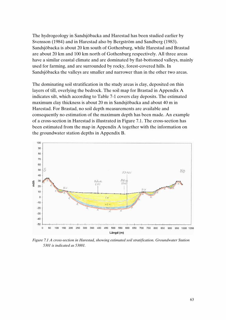
63

The hydrogeology in Sandsjöbacka and Harestad has been studied earlier by Svensson (1984) and in Harestad also by Bergström and Sandberg (1983). Sandsjöbacka is about 20 km south of Gothenburg, while Harestad and Brastad are about 20 km and 100 km north of Gothenburg respectively. All three areas have a similar coastal climate and are dominated by flat-bottomed valleys, mainly used for farming, and are surrounded by rocky, forest-covered hills. In Sandsjöbacka the valleys are smaller and narrower than in the other two areas. The dominating soil stratification in the study areas is clay, deposited on thin layers of till, overlying the bedrock. The soil map for Brastad in Appendix A indicates silt, which according to Table 7-1 covers clay deposits. The estimated maximum clay thickness is about 20 m in Sandsjöbacka and about 40 m in Harestad. For Brastad, no soil depth measurements are available and consequently no estimation of the maximum depth has been made. An example of a cross-section in Harestad is illustrated in Figure 7.1. The cross-section has been estimated from the map in Appendix A together with the information on the groundwater station depths in Appendix B.

Figure 7.1 A cross-section in Harestad, showing estimated soil stratification. Groundwater Station

5301 is indicated as 53001.

64

7.1 Maps, precipitation and temperature For the studies, topographical maps from Lantmäteriverket20 have been used together with soil type maps from SGU21 (see Appendix A). When these maps are superimposed it is clear that they have a minor co-ordinate displacement. The co-ordinates for the groundwater stations have also been found to deviate slightly from the actual positions. Precipitation and temperature data have been taken from the PTHBV22 database at SMHI23. The database contains daily mean values from 1961, interpolated to a 4x4 km grid for the whole of Sweden. The interpolation method, developed by Johansson (2002), considers topography, wind situation and corrections for precipitation measurement errors. In addition to interpolated observations, the database contains climate simulations, carried out at Rossby Centre at SMHI.

7.2 Groundwater levels and pore pressures Groundwater level observations have mainly been taken from the database at SGU, known as the Groundwater Network (SGU, 1985). The Groundwater Network was started in the late 1960s and groundwater levels have since then been measured in open standpipes about twice a month in around 100 areas in Sweden. The case study areas in the Groundwater Network are numbered as: Sandsjöbacka (52), Harestad (53) and Brastad (69). Each area contains several groundwater stations, most of which are placed in unconfined aquifers. In contrast, most of the groundwater stations in the three study areas are located in confined aquifers (see Table 7-1). The stations in Brastad, however, seem to be located with the filters in clay and not in the underlying till. In Sandsjöbacka 14 groundwater stations have been installed, of which six are currently active; in Harestad, seven of the 14 stations are still active and in Brastad all three stations are active. The groundwater levels are measured approximately twice a month although for most of the active stations the observation interval has recently been reduced to once a month. Pictures of groundwater stations in Sandsjöbacka and Harestad are presented in Appendix C. Within this study, pore pressure sensors have also been installed at the groundwater Stations 5301, 5305 and 5310 in Harestad.

20 The Swedish Land Survey Institute 21 The Geological Survey of Sweden 22 Precipitation and Temperature for the HBV model 23 Swedish Meteorological and Hydrological Institute

65

Table 7-1 Stratification and aquifer type for all groundwater stations in Sandsjöbacka, Harestad and Brastad. Active stations, located in confined aquifers, are shown in bold. The stratification is indicated, from the ground level and downwards, with the notations: ‘-‘ (unknown material), S (sand), C (clay), T (till), P (peat). The aquifer type is indicated by: C (confined) or U (unconfined). The stations in Brastad are classified as located in confined aquifers but also as located within the clay layer.

Sandsjöbacka Harestad Brastad

Station Stratification Aquifer type

Station Stratification Aquifer type

Station Stratification Aquifer type

5201 -/S U 5301 C/T C 6902 -/C C

5202 C/T C1 5302 C/T C 6903 -/C C

5203 C/T C 5303 C/T C 6904 -/C C

5204 C/T C 5304 C/T C

5205 S/T U 5305 C/T C

5206 -/S U 5306 C/T C

5207 P/C/T C 5307 C/T C

5208 C/T C 5308 C/T C

5209 P/C/T C 5309 C/T C

5210 C/T C 5310 C/T C

5211 C/T C 5311 C/T C

5212 C/T C 5312 C/T C

5213 C/T C 5313 C/T C

5214 C/T C 5314 C/S C

1 Station 5202 is classified as being located in an unconfined aquifer, which was later found to be

incorrect.

8 ANALYSES OF GROUNDWATER LEVEL OBSERVATIONS

The groundwater level observations from the areas Sandsjöbacka, Harestad and Brastad, introduced in Chapter 7, are analysed in this chapter. The analyses are focused on fluctuation patterns and classification of these. There is also a discussion of the measurement accuracy and the quality of the Groundwater Network data. As mentioned in Chapter 4.1, and illustrated in Figure 8.1, the groundwater levels follow generally the ground level. However, a tendency towards more artesian groundwater levels can be seen for the lower ground levels in each area.

66

Figure 8.1 Maximum and minimum groundwater levels in relation to the ground level for the

groundwater stations in Sandsjöbacka (left) and Harestad (right). The maximum and minimum levels are determined from data series going back more than 10 years.

8.1 Fluctuation patterns Analyses of the groundwater level observation series indicate different fluctuation patterns at different groundwater stations. At some stations the groundwater level fluctuation is large and fast, while in other stations it is small and slow. The groundwater level response to precipitation thus varies considerably between different stations. Classification systems for groundwater stations have been presented in the Groundwater Network (SGU, 1985), by Svensson (1984), and by Bengtsson and Boström (2008). In the Groundwater Network, the hydrogeological position of a station is classified in terms of inflow, intermediate and outflow position (SGU, 1985). According to Svensson (1984), the topographical position of the groundwater stations can be categorised as high or low. Svensson also uses the subcategory side position. The slope can be classified as small, medium and large. However, Svensson does not present any definition of these parameters. Accordance of these two systems could be expected for inflow and high side position, in which the stations with large fluctuation amplitudes should be classified. In addition, accordance could be expected for outflow and low position, for stations with small fluctuations. However, the correlation between the two classification systems is not very strong, as can be seen in Table 8-1, although there is some accordance. The classification system used by Bengtsson and Boström is a simpler form of the classification system presented in this chapter.

35 40 45 50 55 60 6535

40

45

50

55

60

65

Ground level at station [m a.s.l.]

Gro

undw

ater

leve

l [m

a.s

.l.]

Max level

Min level

Groundwater level equals ground level

0 5 10 15 20 25 300

5

10

15

20

25

30

Ground level at station [m a.s.l.]

Gro

undw

ater

leve

l [m

a.s

.l.]

Max level

Min level

Groundwater level equals ground level

67

Table 8-1 Groundwater station classification systems for Sandsjöbacka, Harestad and Brastad. Active stations are displayed in bold. The hydrogeological position is classified as I (inflow), M (intermediate) and O (outflow). The topographical position is classified as L (low) and H (high), with the subcategory S (side) position. The slope is classified as s (small), m (medium) and l (large).

Sandsjöbacka Harestad Brastad

Station Hydro-geological position1

Topo-graphical position2

Slope2 Station Hydro-geological position1

Topo-graphical position2

Slope2 Station Hydro-geological position1

5201 I 5301 O L s 6902 I

5202 I LS M 5302 M LS s-m 6903 I

5203 M 5303 M 6904 I

5204 M HS S 5304 O

5205 I H M 5305 M

5206 I 5306 M

5207 O L S 5307 O L s

5208 O LS M 5308 O

5209 O H M 5309 M L s

5210 O L S 5310 M HS s

5211 O L S 5311 M HS s

5212 O HS S 5312 M

5213 M L S 5313 M HS m

5214 M HS s-m 5314 M

1 From SGU (1985) 2 From Svensson (1984)

Three main fluctuation groups have been identified: one group with quick fluctuations and without a distinct maximum level, one group with rather pronounced maximum levels during wintertime and slower responses, and one group with even slower responses and no distinct maximum levels. The fluctuation patterns are presented in Figure 8.2. In the first group no artesian pressures are present while in the second group all stations except for 6902 and 6903 have artesian pressures. In the last group a few of the stations show pressure levels a little above ground level. The fluctuation patterns for Stations 6902 and 6903 fit best into the second group due to slow responses. The reason for these slow responses is that the station filters are located in clay. Since the stations are located close to infiltration areas the levels are not artesian. There is no obvious agreement between the classifications in Table 8-1 and the fluctuation patterns in Figure 8.2, even though the side position index seems to correlate slightly to the quick fluctuation patterns and all outflow positions are in the slow responding

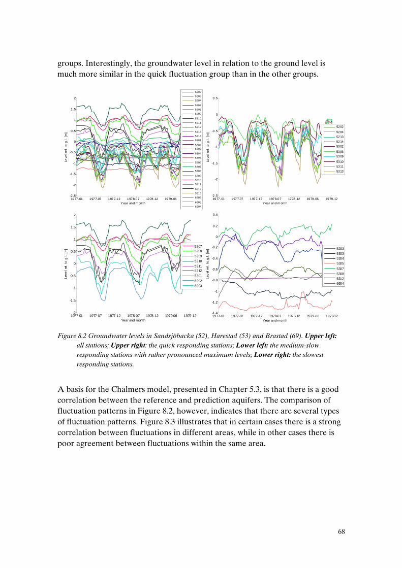
68

groups. Interestingly, the groundwater level in relation to the ground level is much more similar in the quick fluctuation group than in the other groups.

Figure 8.2 Groundwater levels in Sandsjöbacka (52), Harestad (53) and Brastad (69). Upper left:

all stations; Upper right: the quick responding stations; Lower left: the medium-slow responding stations with rather pronounced maximum levels; Lower right: the slowest responding stations.

A basis for the Chalmers model, presented in Chapter 5.3, is that there is a good correlation between the reference and prediction aquifers. The comparison of fluctuation patterns in Figure 8.2, however, indicates that there are several types of fluctuation patterns. Figure 8.3 illustrates that in certain cases there is a strong correlation between fluctuations in different areas, while in other cases there is poor agreement between fluctuations within the same area.

1977-01 1977-07 1977-12 1978-07 1978-12 1979-06 1979-12-2 .5

-2

-1 .5

-1

-0 .5

0

0.5

1

1.5

2

Leve

l re

l. to

g.l

. [m

]

Y ear and m onth

5202

5203

5204

5207

5208

5209

5210

5211

5212

5213

5214

5301

53025303

5304

5305

5306

5307

5308

5309

5310

5311

5312

5313

6902

6903

6904

1977-01 1977-07 1977-12 1978-07 1978-12 1979-06 1979-12-2 .5

-2

-1 .5

-1

-0 .5

0

0.5

Leve

l re

l. to

g.l

. [m

]Y ear and m onth

5202

5204

5213

5214

5302

5306

5309

5310

5311

5313

1977-01 1977-07 1977-12 1978-07 1978-12 1979-06 1979-12-1.4

-1.2

-1

-0.8

-0.6

-0.4

-0.2

0

0.2

0.4

Leve

l rel

. to

g.l.

[m]

Year and month

5203530353045305

5307530853126904

1977-01 1977-07 1977-12 1978-07 1978-12 1979-06 1979-12-2

-1.5

-1

-0.5

0

0.5

1

1.5

2

Leve

l rel

. to

g.l.

[m]

Year and month

520752085209521052115212530169026903

69

Figure 8.3 Groundwater level observations from Sandsjöbacka (52) and Harestad (53). Left: good

agreement between certain stations in the two areas; Right: poor agreement within the Harestad area; note the phase offset.

8.2 Accuracy of the open standpipe measurements There are several measurement techniques for observation of groundwater levels, of which open standpipes and closed pore pressure gauging systems are the two main types. Open standpipes, with a filter at the lower end, are common for measuring groundwater levels in materials with relatively high permeability. For measurements in materials with low permeability, such as clay, the response in open standpipes is too slow to pick up quick pressure changes. This is due to the fact that the water volume entering (or exiting) the pipe, required to indicate a pressure change correctly is larger than the low permeable soil can transport within the time of the pressure change. A low-volume system is therefore needed for measurements in low permeable soils. In this study the BAT system has been used, which is a closed system where only a very small volume change in the gauge is needed to give a correct pressure indication (BAT, 2008). Open and closed systems have been compared in several studies. Bergdahl and Tremblay (1987) conclude that the seasonal groundwater variations can also be measured using open systems in a clay deposit (see Figure 8.4). Tremblay (1990), however, stresses that open standpipes cannot be used for short-term effects in low permeability material. In contrast, a study by Larsson and Åhnberg (2003) found that open systems in clay also gave an averaged response, without maximum and minimum levels, for long-term measurements (see Figure 8.4).

1977-01 1977-07 1977-12 1978-07 1978-12 1979-06 1979-12-2.5

-2

-1.5

-1

-0.5

0

0.5

Leve

l rel

. to

g.l.

[m]

Year and month

53115312

1977-01 1977-07 1977-12 1978-07 1978-12 1979-06 1979-12-2.5

-2

-1.5

-1

-0.5

0

0.5

1

1.5

Leve

l re

l. to

g.l

. [m

]

Year and m onth

5207

5214

5301

5311

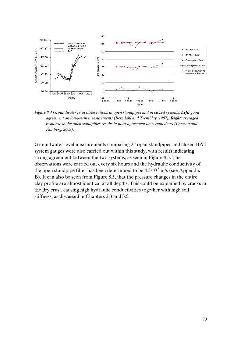
70

Figure 8.4 Groundwater level observations in open standpipes and in closed systems. Left: good

agreement on long-term measurements (Bergdahl and Tremblay, 1987); Right: averaged response in the open standpipes results in poor agreement on certain dates (Larsson and Åhnberg, 2003).

Groundwater level measurements comparing 2” open standpipes and closed BAT system gauges were also carried out within this study, with results indicating strong agreement between the two systems, as seen in Figure 8.5. The observations were carried out every six hours and the hydraulic conductivity of the open standpipe filter has been determined to be 4.5·10-8 m/s (see Appendix B). It can also be seen from Figure 8.5, that the pressure changes in the entire clay profile are almost identical at all depths. This could be explained by cracks in the dry crust, causing high hydraulic conductivities together with high soil stiffness, as discussed in Chapters 2.3 and 3.5.

71

2007-07-01 2007-07-19 2007-08-06 2007-08-24 2007-09-11 2007-09-29-70

-60

-50

-40

-30

-20

-10Le

vel [

cm r

el.

to g

.l.]

6m

9m3m

5310

Figure 8.5 Measurements from closed pore pressure gauges and an open standpipe at Station 5310

in Harestad. Pore pressure observations are made at 3, 6 and 9 m depth below ground level. The open standpipe filter is also located at a depth of 9 m.

A hypothetical explanation for the high level of agreement between the open and closed systems in this study, as well as in the study by Bergdahl and Tremblay (1987), could be that the closed gauges were installed too close to the open standpipe, which governs the groundwater level in the vicinity of the open standpipe through the water level in the pipe. This hypothesis has, however, not been tested and evaluated. Another important aspect of the recorded groundwater fluctuations is the observation frequency. When observations are made too infrequently, the maximum and minimum levels could be missed, as illustrated in Figure 8.6.

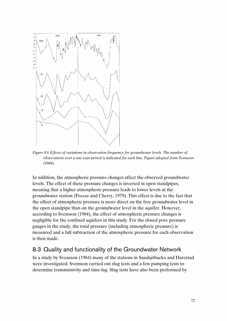
72

Figure 8.6 Effects of variations in observation frequency for groundwater levels. The number of

observations over a one-year period is indicated for each line. Figure adopted from Svensson (1984).

In addition, the atmospheric pressure changes affect the observed groundwater levels. The effect of these pressure changes is inverted in open standpipes, meaning that a higher atmospheric pressure leads to lower levels at the groundwater station (Freeze and Cherry, 1979). This effect is due to the fact that the effect of atmospheric pressure is more direct on the free groundwater level in the open standpipe than on the groundwater level in the aquifer. However, according to Svensson (1984), the effect of atmospheric pressure changes is negligible for the confined aquifers in this study. For the closed pore pressure gauges in the study, the total pressure (including atmospheric pressure) is measured and a full subtraction of the atmospheric pressure for each observation is then made.

8.3 Quality and functionality of the Groundwater Network In a study by Svensson (1984) many of the stations in Sandsjöbacka and Harestad were investigated. Svensson carried out slug tests and a few pumping tests to determine transmissivity and time-lag. Slug tests have also been performed by

73

SGU (in 2002 and 2005), by SGI (in 2008) and by Bengtsson and Boström (2008). Svensson as well as Bengtsson and Boström also measured the station depths. Many of the depth measurements indicated reduced depths in relation to the installation depths (see Appendix B). The reasons for this could be silted-up filters, shortened pipes and in some exceptional cases possible broken pipes. The slug tests have been evaluated using the Hvorslev method, see e.g. Fetter (1994). The test results generally indicated reduced hydraulic conductivities in the open standpipe filter and its surroundings in relation to earlier investigations (see Appendix B). The determined hydraulic conductivities fall into the range 10-5–10-

9 m/s. The hydraulic conductivity decrease could also have been caused by silted-up filters. A comparison of the groundwater Stations 5214 and 5211, with the filter hydraulic conductivities 1.8·10-6 m/s and 1.8·10-8 m/s respectively (see Appendix B) indicates large difference in response time. An instantaneous groundwater level rise in the soil caused, within 10 minutes, a level change in Station 5214 corresponding to 95% of the total change. At Station 5211, on the other hand, the response within 10 minutes was only 3% of the total change (Bengtsson and Boström, 2008). Consequently, the hydraulic conductivity affects the response time and thus also the fluctuation pattern. Stations with low hydraulic conductivity have slow fluctuation patterns in comparison with stations with high conductivity. This effect might contribute to the difference in fluctuation patterns seen in Figure 8.2, which mainly is caused by differences in station locations. At three of the stations in Harestad: 5301, 5305 and 5310, geotechnical soundings and installation of pore pressure gauges have also been carried out. The soundings at 5301 and 5310 confirmed the soil profile given in Table 7-1 and the depths given in Appendix B, while at 5305 the sounding indicated clay layers reaching 10 m below the filter level for the station. The groundwater station filter at 5305 is thus located in clay and not in the underlying aquifer, as indicated in Table 7-1. This result was not entirely surprising, since the fluctuation pattern at this station is very slow and the slug tests indicated very low hydraulic conductivity. The pore pressure observations from Stations 5301, 5305 and 5310 indicated pressure levels in agreement with the groundwater level observations in the open standpipes. Unfortunately, many other factors also affect the Groundwater Network data and the data quality is sometimes low. Data series do not appear to have been checked for measurement errors, e.g. where presumably two stations have been

74

mixed up. In some cases the reference level has been changed due to frost heave, settlement or changed pipe length. Occasionally, standpipes that were too short were installed, causing a flowing pipe and thus obviously a maximum level that was too low. Many of the groundwater level series also show heterogeneity over time, the reason for which in most cases is unknown. Examples of these data errors are shown in Figure 8.7.

Figure 8.7 Examples of data observation series from the Groundwater Network containing incorrect

measurements. Top left: the observations from Stations 5306 and 5307 appear to be mixed up; Top right: the observations from Station 5305 show strong heterogeneity in amplitude over time; Bottom left: the reference level appears to have been changed in Station 5208; Bottom right: a distinct maximum level due to overflow at Station 5211.

Bengtsson and Boström (2008) recommend that only Stations 5202, 5208, 5209, 5213, 5214, 5310 and 5311 be used for predictions using the Chalmers model. This recommendation was based on requirements for homogeneity of the data series and reasonably high hydraulic conductivities of the station filters.

1971-06 1977-07 1983-08 1989-08 1995-09 2001-10 2007-11-2

-1.8

-1.6

-1.4

-1.2

-1

-0.8

-0.6

-0.4

-0.2

0

Leve

l rel

. to

g.l.

[m]

Year and month

5305

1971-06 1977-07 1983-08-0.4

-0.2

0

0.2

0.4

0.6

0.8

1

1.2

1.4

1.6

Leve

l rel

. to

g.l.

[m]

Year and mont h

5208

1989-08 1995-09

-0.4

-0.2

0

0.2

0.4

0.6

Leve

l rel

. to

g.l.

[m

]

Year and month

5211

1971-06 1977-07 1983-08 1989-08 1995-09 2001-10 2007-11-2

-1.5

-1

-0.5

0

0.5

1

1.5

Lev

el r

el.

to g

.l. [

m]

Y ear and m onth

5306

5307

75

9 RESULTS FROM SIMULATIONS USING THE MODIFIED HBV MODEL

Groundwater levels have been simulated for confined aquifers in the study areas Sandsjöbacka, Harestad and Brastad, with the aim of improving the classification systems for groundwater stations discussed in Chapter 8.1. The simulations have been carried out using the modified HBV model, presented in Chapter 6. An example of input and output data for the model is presented in Appendix D. Calibration of the modified HBV model has been done for all active groundwater stations in the Groundwater Network in the case study areas. The main focus in the calibrations has been on capturing the high groundwater levels, which sometimes results in a less accurate description of the lower levels. It should also be noted that the model is calibrated for the observed groundwater fluctuations at the stations, which can differ from the real fluctuations in the open standpipes. These differences are caused partly by the fact that the two-week observation interval does not always describe the real fluctuations, as shown in Figure 8.6. Moreover – also discussed in Chapters 8.2 and 8.3 – the fluctuations in the groundwater stations do not necessarily correspond to the real groundwater level fluctuations. The geological information available for the Groundwater Network stations is quite limited, meaning that the new classification system must be simple and be based on generally available information. Consequently, simple criteria are suggested that can be identified easily from, for example, topographical and soil type maps. A new classification system and application of the system to the groundwater stations in Sandsjöbacka, Harestad and Brastad are presented in the following chapters. In addition, the model parameter values from the calibrations have been compared with the classification of the groundwater stations. A correlation between classification and model parameters was found and was used for validation of the model at the Groundwater Network's non-active stations. The reason for the termination of the non-active stations is not known and only data that is considered to be correct has been used. In the validation process, the aim has been to adopt an objective approach and not make use of prior knowledge of the fluctuation patterns, from Chapter 8.1 for example. A general discussion of the calibration and validation results is presented in Chapter 9.5.

76

9.1 A revised classification system for groundwater level fluctuations

A revised system is suggested for classification of groundwater fluctuation patterns in categories similar to the fluctuation patterns in Figure 8.2. The new system is based on the classification systems discussed in Chapter 8.1, although developed further. The main parts of the system are distance to the infiltration areas, size and steepness of these areas, distance to the downstream groundwater level boundary and the estimated stability, or lack of variation, of this boundary. As discussed in Chapter 4.3, the aquifer size also affects the fluctuation patterns. The aquifers in the study areas are relatively small and the size of the aquifer has therefore not been included directly in the classification system. However, the stability of the downstream pressure boundary is affected by the aquifer size, meaning that the size is considered indirectly. The classification of the stations was done from map and field analyses. Maps are found in Appendix A. The classification of the groundwater stations was done individually for each area, meaning that the classification values (1–3) are related to each specific area, and thus that the same classification value not necessarily represent entirely the same situation in different areas. In Table 9-1, properties affecting the fluctuation patterns are presented together with the classification criteria. The table also contains the links between the classification parameters and the modified HBV model parameters.

Table 9-1 Properties affecting the groundwater fluctuation patterns and suggested criteria for classification, together with the related parameters in the modified HBV model.

Position1 Property affecting the

fluctuation pattern

Suggested

criteria

Classification

value (1-3)

Related

parameter in

the modified

HBV model

Amount of precipitation that reaches the infiltration zone

Time delay of infiltrated water

Distance and elevation difference to infiltration areas and their size and steepness

3 for stations close to large and steep infiltration areas, and 1 for stations with opposite conditions

kuz

Overflow level in infiltration zone

Lowest level in the infiltration zone

- llz,overflow

Infiltration areas

Overflow capacity in the infiltration zone

Size and permeability of the infiltration

- klz,overflow

77

zone at overflow level

Downstream flow capacity from the groundwater station

Aquifer

Stability of the downstream groundwater level boundary

Distance and elevation difference to the valley bottom and the stability of the downstream groundwater level boundary

1 for stations close to a large and stable downstream groundwater level boundary, and 3 for stations with the opposite conditions

klz

1 The position for the physical processes and the position in the modified HBV model are not always corresponding, as discussed in Chapter 6.3.

The classification leaves scope for a considerable degree of subjectivity and each criterion contains several parameters. For the kuz criterion, the distance to the infiltration area is considered most important. For the klz criterion the distance to the valley bottom is considered most important. Exemplifying the classification usage can be done using the fluctuations in Figure 8.2. The rapidly responding fluctuation patterns are examples of stations with high classification values for kuz and klz. For the slowest responding stations the opposite is true, and the classification values are typically low for both kuz and klz.

9.2 Sandsjöbacka In this chapter a classification of the groundwater stations in Sandsjöbacka is presented, together with calibration simulations and validation simulations using the modified HBV model.

9.2.1 Model calibration The stations were calibrated for the period 1975–1980, except for station 5213, which was calibrated for the period 1973–1978. The reason for the varying calibration periods is heterogeneity in the groundwater level observation series. The periods estimated as being most correct were chosen as calibration periods. The model was found to describe the fluctuation patterns quite satisfactorily, as can be seen in Figure 9.1. For an illustration of all calibrated stations, see Appendix E.

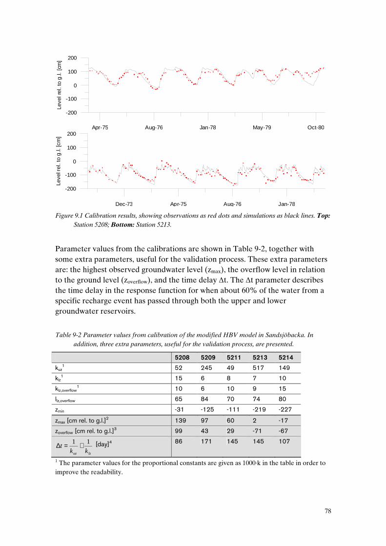
78

Figure 9.1 Calibration results, showing observations as red dots and simulations as black lines. Top:

Station 5208; Bottom: Station 5213.

Parameter values from the calibrations are shown in Table 9-2, together with some extra parameters, useful for the validation process. These extra parameters are: the highest observed groundwater level (zmax), the overflow level in relation to the ground level (zoverflow), and the time delay ∆t. The ∆t parameter describes the time delay in the response function for when about 60% of the water from a specific recharge event has passed through both the upper and lower groundwater reservoirs.

Table 9-2 Parameter values from calibration of the modified HBV model in Sandsjöbacka. In addition, three extra parameters, useful for the validation process, are presented.

5208 5209 5211 5213 5214

kuz1 52 245 49 517 149

klz1 15 6 8 7 10

klz,overflow1 10 6 10 9 15

llz,overflow 65 84 70 74 80

zmin -31 -125 -111 -219 -227

zmax [cm rel. to g.l.]2 139 97 60 2 -17

zoverflow [cm rel. to g.l.]3 99 43 29 -71 -67

lzuz kkt

11 +=∆ [day]4 86 171 145 145 107

1 The parameter values for the proportional constants are given as 1000·k in the table in order to improve the readability.

Dec-73 Apr-75 Aug-76 Jan-78

-200

-100

0

100

200

Leve

l rel

. to

g.l.

[cm

]

Apr-75 Aug-76 Jan-78 May-79 Oct-80

-200

-100

0

100

200Le

vel r

el. t

o g

.l. [

cm]

79

2 Maximum observed groundwater level. 3 Overflow level related to the ground level, calculated from equation 6.3 as zoverflow=zgw(llz,overflow). 4 Time delay, indicating the delay through the response routine when ~60% of the water has passed.

The outflow coefficient from the upper groundwater reservoir, kuz, varies by more than a factor of 10 between the stations, while the corresponding coefficient for the lower reservoir, klz, varies by a factor of 2.5. Large values of kuz mean a rapid groundwater level response to recharge. As seen from Table 9-2 and maps in Appendix A, the stations with the highest kuz values are located close to infiltration areas and are thus also expected to show rapid fluctuation patterns. Moreover, the coefficients kuz and klz seem to have a negative correlation, i.e. meaning that klz is small when kuz is large. This means that the time ∆t, presented in Table 9-2, does not vary by more than a factor of two between all stations. The zmin parameter varies between the stations depending on the local geology, with the largest negative values for the stations close to infiltration areas, i.e. where large fluctuations can be expected. The llz,overflow parameter varies by a factor of 1.3, but with a tendency towards higher values for the stations close to infiltration areas. The zoverflow parameter is also related to the maximum groundwater level, zmax, at each station, as seen in Table 9-2, and can naturally not exceed the maximum groundwater level. Moreover, the overflow parameter klz,overflow varies by a factor of 2.5, without any clear pattern.

9.2.2 Classification and model parameter evaluation The active stations in Sandsjöbacka have been classified according to the system presented in Chapter 9.1. The classification values are presented in Table 9-3 together with the calibration results for the parameters kuz and klz.

Table 9-3 Classification values for active stations in Sandsjöbacka, together with calibration results for kuz and klz.

5208 5209 5211 5213 5214

Distance and elevation difference to infiltration areas and their size and steepness

1 3 1 3 2

kuz1 52 245 59 517 149

Distance and elevation difference to the valley bottom and the stability of the downstream groundwater level boundary

1 2 1 3 2

klz1 15 6 8 7 10

1 The parameter values for the proportional constants are given as 1000·k in the table in order to improve the readability.

80

Based on the relationship between the calibration values and the classification values, a parameter set-up has been identified, with specific values for kuz and klz, representing each classification value. When identifying the specific values for kuz and klz, the aim has also been to keep the parameter ∆t within the range 100-130 days, which is in the middle of the calibration range for ∆t (see Table 9-2). The identified standard parameter set-up is presented in Table 9-4, and has later been used for the validation. The choice of parameter value for zmin must be based on general hydrogeological experience of the lowest levels in the area but can be improved substantially using one or a few groundwater level observations. Equally, the llz,overflow (or zoverflow) must be based on general hydrogeological experience of the overflow levels in the area (i.e. information from the other groundwater stations). However, zoverflow can also be related to the estimated maximum groundwater level, which in turn must be based on hydrogeological experience from the area. For klz,overflow, the parameter value has been estimated as being equal to 10. This choice also reflects the difficulty of identifying a physical explanation for klz,overflow, which led to the choice of a fixed parameter value.

Table 9-4 Estimated parameter values for validation of the modified HBV model in Sandsjöbacka. Each classification value has a corresponding parameter value.

Classification value Identified parameter value

1 50

2 150

kuz1

3 300

1 12

2 10

klz1

3 8

klz,overflow1 - 10

llz,overflow - From hydrogeological experience, although zoverflow can also be related to the estimated maximum groundwater level.

zmin - From hydrogeological experience and/or one or a few groundwater observations.

1 The parameter values for the proportional constants are given as 1000·k in the table in order to improve the readability.

9.2.3 Model validation The non-active groundwater stations in Sandsjöbacka were assigned classification values according to Chapter 9.1, based on map analyses, and are shown in Table 9-5.

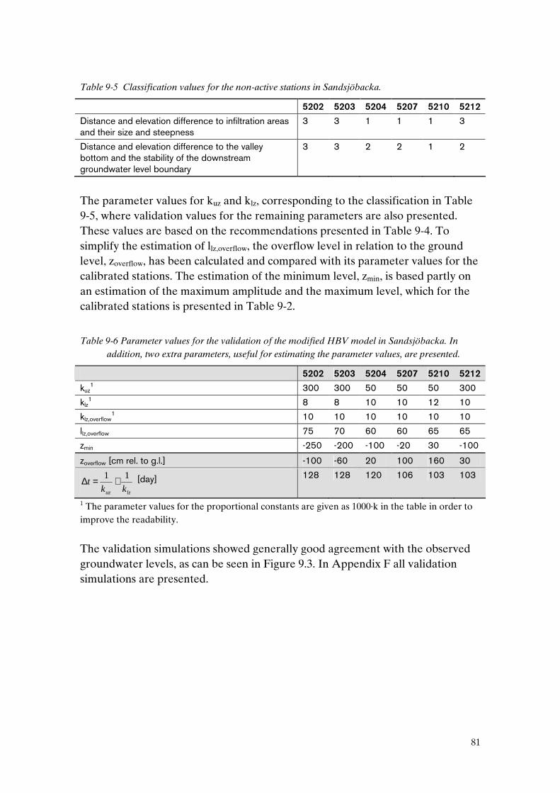
81

Table 9-5 Classification values for the non-active stations in Sandsjöbacka.

5202 5203 5204 5207 5210 5212

Distance and elevation difference to infiltration areas and their size and steepness

3 3 1 1 1 3

Distance and elevation difference to the valley bottom and the stability of the downstream groundwater level boundary

3 3 2 2 1 2

The parameter values for kuz and klz, corresponding to the classification in Table 9-5, where validation values for the remaining parameters are also presented. These values are based on the recommendations presented in Table 9-4. To simplify the estimation of llz,overflow, the overflow level in relation to the ground level, zoverflow, has been calculated and compared with its parameter values for the calibrated stations. The estimation of the minimum level, zmin, is based partly on an estimation of the maximum amplitude and the maximum level, which for the calibrated stations is presented in Table 9-2.

Table 9-6 Parameter values for the validation of the modified HBV model in Sandsjöbacka. In addition, two extra parameters, useful for estimating the parameter values, are presented.

5202 5203 5204 5207 5210 5212

kuz1 300 300 50 50 50 300

klz1 8 8 10 10 12 10

klz,overflow1 10 10 10 10 10 10

llz,overflow 75 70 60 60 65 65

zmin -250 -200 -100 -20 30 -100

zoverflow [cm rel. to g.l.] -100 -60 20 100 160 30

lzuz kkt

11 +=∆ [day] 128 128 120 106 103 103

1 The parameter values for the proportional constants are given as 1000·k in the table in order to improve the readability.

The validation simulations showed generally good agreement with the observed groundwater levels, as can be seen in Figure 9.3. In Appendix F all validation simulations are presented.

82

Apr-75 Aug-76 Jan-78 May-79 Oct-80

-200

-100

0

100

200Le

vel r

el. t

o g

.l. [c

m]

Figure 9.2 Validation results for Station 5212, showing observations as red dots and simulations as a

black line.

For Station 5204 the estimated classification was found to be highly incorrect and needed to be modified to describe the observations satisfactorily. The main reason for this was an assumption of the lake west of Station 5204 as a much stronger governing boundary condition than it appeared to be. Consequently, the fluctuation pattern was more rapid and had a larger amplitude than expected. In addition, the pressure levels were also much lower than expected. In Figure 9.3 the original simulation is shown together with one modified simulation where zmin has been changed according to one fictive groundwater observation, and with one simulation where other parameters are also modified. The original and the modified parameters are presented in Table 9-7. It is also clear from Figure 9.3 that to estimate the maximum levels the description of the lower levels is not essential.

83

Figure 9.3 Validation results for Station 5204. Upper: with original parameter estimations; Middle:

with level correction from a fictive groundwater level observation on January 17, 1974; Lower: with the best fit parameter values.

Table 9-7 Modified parameter values for Station 5204.

5204 (original) 5204 (one level

observed)

5204 (best fit)

kuz1 50 50 150

zoverflow [cm rel. to g.l.] 20 20 -50

llz,overflow [mm] 60 60 75

zmin [cm rel. to g.l.] -100 -166 -200 1 The parameter values for the proportional constants are given as 1000·k in the table in order to improve the readability.

9.3 Harestad In this chapter a classification of the groundwater stations in Harestad is presented, together with calibration simulations and validation simulations using the modified HBV model.

Mar-71 Jul-72 Dec-73 Apr-75 Aug-76

-200

-100

0

100

200Lev

el rel.

to g

.l. [

cm

]

Mar-71 Jul-72 Dec-73 Apr-75 Aug-76

-200

-100

0

100

200

Lev

el rel.

to g

.l. [

cm

]

Mar-71 Jul-72 Dec-73 Apr-75 Aug-76

-200

-100

0

100

200

Leve

l rel

. to

g.l.

[cm

]

84

9.3.1 Model calibration The Stations 5301, 5310 and 5311 were calibrated for the period 1974–1978, Station 5303 for 1980–1984, Station 5305 for 1977–1979, Station 5306 for 1971–1975 and Station 5307 for 1972–1976. The reason for the varying calibration periods is heterogeneity in the groundwater level observation series. The periods estimated as being most correct were chosen as calibration periods. The model was found to describe the fluctuation patterns quite satisfactorily, as can be seen in Figure 9.4. For an illustration of all calibrated stations, see Appendix E.

Figure 9.4 Calibration results, showing observations as red dots and simulations as black lines. Top:

Station 5301; Bottom: Station 5311.

Parameter values from the calibrations are shown in Table 9-8, together with some extra parameters, useful for the validation process. These extra parameters are: the highest observed groundwater level (zmax), the overflow level in relation to the ground level (zoverflow), and the time delay ∆t. The ∆t parameter describes the time delay in the response function for when about 60% of the water from a specific recharge event has passed through both the upper and lower groundwater reservoirs.

Table 9-8 Parameter values from calibration of the modified HBV model in Harestad. In addition three extra parameters, useful for the validation process are presented.

5301 5303 5305 5306 5307 5310 5311

kuz1 9 5 5 90 10 95 150

Jun-74 Jul-75 Aug-76 Oct-77 Nov-78

-200

-100

0

100

200

Leve

l rel

. to

g.l.

[cm

]

Jun-74 Jul-75 Aug-76 Oct-77 Nov-78

-200

-100

0

100

200

Leve

l rel

. to

g.l.

[cm

]

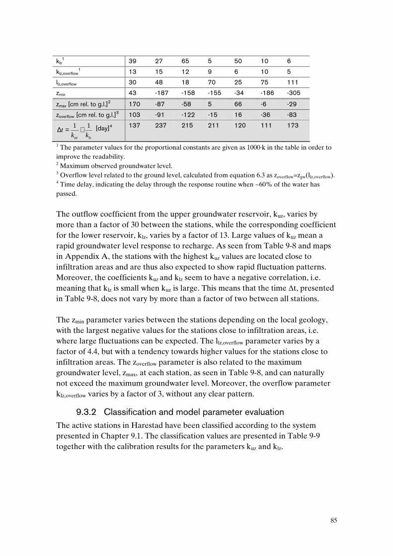
85

klz1 39 27 65 5 50 10 6

klz,overflow1 13 15 12 9 6 10 5

llz,overflow 30 48 18 70 25 75 111

zmin 43 -187 -158 -155 -34 -186 -305

zmax [cm rel. to g.l.]2 170 -87 -58 5 66 -6 -29

zoverflow [cm rel. to g.l.]3 103 -91 -122 -15 16 -36 -83

lzuz kkt

11 +=∆ [day]4 137 237 215 211 120 111 173

1 The parameter values for the proportional constants are given as 1000·k in the table in order to improve the readability. 2 Maximum observed groundwater level. 3 Overflow level related to the ground level, calculated from equation 6.3 as zoverflow=zgw(llz,overflow). 4 Time delay, indicating the delay through the response routine when ~60% of the water has passed.

The outflow coefficient from the upper groundwater reservoir, kuz, varies by more than a factor of 30 between the stations, while the corresponding coefficient for the lower reservoir, klz, varies by a factor of 13. Large values of kuz mean a rapid groundwater level response to recharge. As seen from Table 9-8 and maps in Appendix A, the stations with the highest kuz values are located close to infiltration areas and are thus also expected to show rapid fluctuation patterns. Moreover, the coefficients kuz and klz seem to have a negative correlation, i.e. meaning that klz is small when kuz is large. This means that the time ∆t, presented in Table 9-8, does not vary by more than a factor of two between all stations. The zmin parameter varies between the stations depending on the local geology, with the largest negative values for the stations close to infiltration areas, i.e. where large fluctuations can be expected. The llz,overflow parameter varies by a factor of 4.4, but with a tendency towards higher values for the stations close to infiltration areas. The zoverflow parameter is also related to the maximum groundwater level, zmax, at each station, as seen in Table 9-8, and can naturally not exceed the maximum groundwater level. Moreover, the overflow parameter klz,overflow varies by a factor of 3, without any clear pattern.

9.3.2 Classification and model parameter evaluation The active stations in Harestad have been classified according to the system presented in Chapter 9.1. The classification values are presented in Table 9-9 together with the calibration results for the parameters kuz and klz.

86

Table 9-9 Classification values for active stations in Harestad, together with calibration results for kuz and klz.

5301 5303 5305 5306 5307 5310 5311

Distance and elevation difference to infiltration areas and their size and steepness

1 1 1 2 2 3 3

kuz1 9 5 5 90 10 95 150

Distance and elevation difference to the valley bottom and the stability of the downstream groundwater level boundary

1 3 2 2 1 3 3

klz1 39 27 65 5 50 10 6

1 The parameter values for the proportional constants are given as 1000·k in the table in order to improve the readability.

Based on the relationship between the calibration values and the classification values, a parameter set-up has been identified, with specific values for kuz and klz, representing each classification value. When identifying the specific values for kuz and klz, the aim has also been to keep the parameter ∆t within the range 110–150 days, which is in the middle of the calibration range for ∆t for the stations estimated to have the best functionality (see Table 9-8). The identified standard parameter set-up is presented in Table 9-10, and has later been used for the validation. The choice of parameter value for zmin must be based on general hydrogeological experience of the lowest levels in the area but can be improved substantially using one or a few groundwater level observations. Equally, the llz,overflow (or zoverflow) must be based on general hydrogeological experience of the overflow levels in the area (i.e. information from the other groundwater stations). However, zoverflow can also be related to the estimated maximum groundwater level, which in turn must be based on hydrogeological experience from the area. For klz,overflow, the parameter value has been estimated as being equal to 10. This choice also reflects the difficulty of identifying a physical explanation for klz,overflow, which led to the choice of a fixed parameter value.

Table 9-10 Estimated parameter values for validation of the modified HBV model in Harestad. Each classification value has a corresponding parameter value.

Classification value Identified parameter value

1 10

2 50

kuz1

3 120

1 40

2 10

klz1

3 8

klz,overflow1 - 10

87

llz,overflow - From hydrogeological experience, although zoverflow can also be related to the estimated maximum groundwater level.

zmin - From hydrogeological experience and/or one or a few groundwater observations.

1 The parameter values for the proportional constants are given as 1000·k in the table in order to improve the readability.

9.3.3 Model validation The non-active groundwater stations in Harestad were assigned classification values according to Chapter 9.1, based on map analyses, and are shown in Table 9-11.

Table 9-11 Classification values for the non-active stations in Harestad.

5302 5304 5308 5309 5312 5313

Distance and elevation difference to infiltration areas and their size and steepness

3 1 1 2 3 3

Distance and elevation difference to the valley bottom and the stability of the downstream groundwater level boundary

3 1 1 3 2 3

The parameter values for kuz and klz, corresponding to the classification in Table 9-11, where validation values for the remaining parameters are also presented. These values are based on the recommendations presented in Table 9-10. To simplify the estimation of llz,overflow, the overflow level in relation to the ground level, zoverflow, has been calculated and compared with its parameter values for the calibrated stations. The estimation of the minimum level, zmin, is based partly on an estimation of the maximum amplitude and the maximum level, which for the calibrated stations is presented in Table 9-8.

Table 9-12 Parameter values for the validation of the modified HBV model in Harestad. In addition, two extra parameters, helpful for estimation of the parameter values are presented.

5302 5304 5308 5309 5312 5313

kuz1 120 10 10 50 120 120

klz1 8 40 40 8 10 8

klz,overflow1 10 10 10 10 10 10

llz,overflow 85 40 35 75 75 85

zmin -250 -20 30 -200 -200 -250

zoverflow [cm rel. to g.l.] -80 60 100 -50 -50 -80

lzuz kkt

11 +=∆ [day] 133 125 125 145 108 133

88

1 The parameter values for the proportional constants are given as 1000·k in the table in order to improve the readability.

The validation simulations showed good agreement with the observed groundwater levels for three out of six simulations. In Figure 9.5 one of the better validations is illustrated, and in Appendix F all validation simulations are presented.

Jul-75 Aug-76 Oct-77 Nov-78 Dec-79

-200

-100

0

100

200

Lev

el r

el.

to g

.l. [c

m]

Figure 9.5 Validation results for Station 5302, showing observations as red dots and simulations as a

black line.

For the Stations 5304, 5308 and 5312 the estimated classification was found to be highly incorrect and needed to be modified to describe the observations satisfactorily. For the Stations 5304 and 5308 the fluctuation amplitudes were smaller than expected and the pressure levels, especially for 5308, were overestimated. This means that the governing downstream boundary conditions were stronger than expected. Further, Station 5312 had unexpectedly small variation and an odd phase-shift, leading to suspicions of the station as malfunctioning. In Figure 9.6 the original simulation for Station 5308 is shown together with one modified simulation where zmin has been changed according to one fictive groundwater observation, and with one simulation where other parameters are also modified. In addition, the original and the modified parameters for the Stations 5304, 5308 and 5312 are presented in Table 9-13. It is also clear from Figure 9.6 that to estimate the maximum levels, the description of the lower levels is not essential.

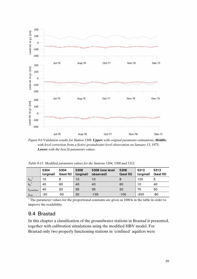
89

Figure 9.6 Validation results for Station 5308. Upper: with original parameter estimations; Middle:

with level correction from a fictive groundwater level observation on January 13, 1975; Lower: with the best fit parameter values.

Table 9-13 Modified parameter values for the Stations 5304, 5308 and 5312.

5304

(orginal)

5304

(best fit)

5308

(orginal)

5308 (one level

observed)

5308

(best fit)

5312

(orginal)

5312

(best fit)

kuz1 10 8 10 10 8 120 5

klz1 40 60 40 40 60 10 40

llz,overflow 40 20 35 35 20 75 50

zmin -20 -50 30 -135 -100 -200 -80 1 The parameter values for the proportional constants are given as 1000·k in the table in order to improve the readability

9.4 Brastad In this chapter a classification of the groundwater stations in Brastad is presented, together with calibration simulations using the modified HBV model. For Brastad only two properly functioning stations in 'confined' aquifers were

Jul-75 Aug-76 Oct-77 Nov-78 Dec-79

-200

-100

0

100

200L

eve

l re

l. to

g.l.

[cm

]

Jul-75 Aug-76 Oct-77 Nov-78 Dec-79

-200

-100

0

100

200

Lev

el r

el.

to g

.l. [c

m]

Jul-75 Aug-76 Oct-77 Nov-78 Dec-79

-200

-100

0

100

200

Leve

l rel

. to

g.l.

[cm

]

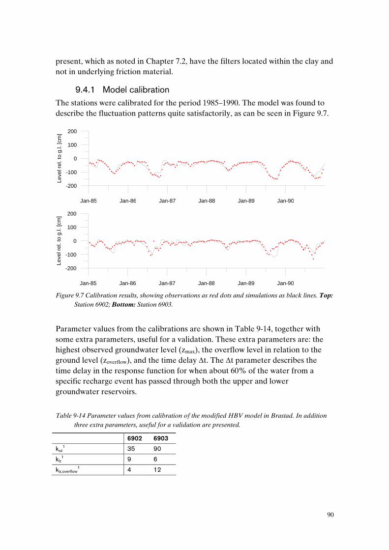
90

present, which as noted in Chapter 7.2, have the filters located within the clay and not in underlying friction material.

9.4.1 Model calibration The stations were calibrated for the period 1985–1990. The model was found to describe the fluctuation patterns quite satisfactorily, as can be seen in Figure 9.7.

Figure 9.7 Calibration results, showing observations as red dots and simulations as black lines. Top:

Station 6902; Bottom: Station 6903.

Parameter values from the calibrations are shown in Table 9-14, together with some extra parameters, useful for a validation. These extra parameters are: the highest observed groundwater level (zmax), the overflow level in relation to the ground level (zoverflow), and the time delay ∆t. The ∆t parameter describes the time delay in the response function for when about 60% of the water from a specific recharge event has passed through both the upper and lower groundwater reservoirs.

Table 9-14 Parameter values from calibration of the modified HBV model in Brastad. In addition three extra parameters, useful for a validation are presented.

6902 6903

kuz1 35 90

klz1 9 6

klz,overflow1 4 12

Jan-85 Jan-86 Jan-87 Jan-88 Jan-89 Jan-90

-200

-100

0

100

200

Leve

l rel

. to

g.l.

[cm

]

Jan-85 Jan-86 Jan-87 Jan-88 Jan-89 Jan-90

-200

-100

0

100

200

Leve

l rel

. to

g.l.

[cm

]

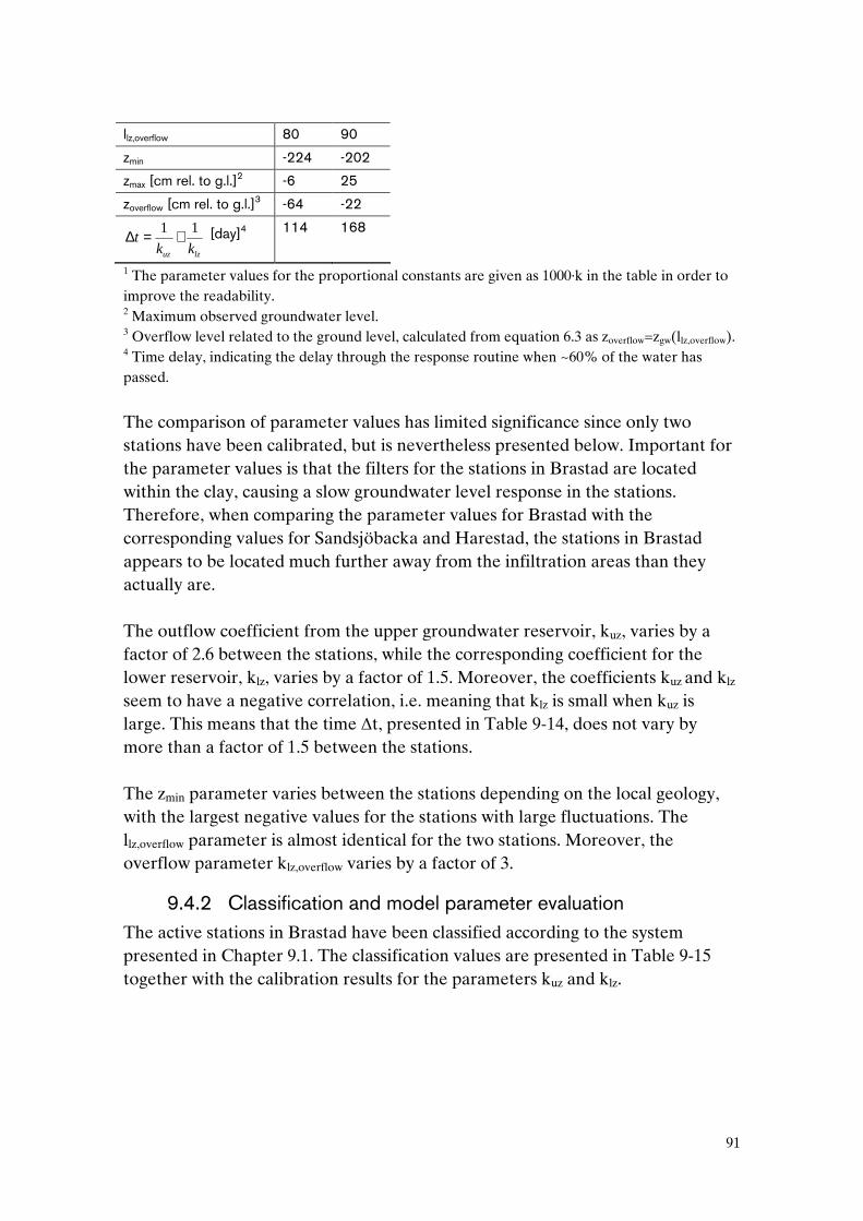
91

llz,overflow 80 90

zmin -224 -202

zmax [cm rel. to g.l.]2 -6 25

zoverflow [cm rel. to g.l.]3 -64 -22

lzuz kkt

11 +=∆ [day]4 114 168

1 The parameter values for the proportional constants are given as 1000·k in the table in order to improve the readability. 2 Maximum observed groundwater level. 3 Overflow level related to the ground level, calculated from equation 6.3 as zoverflow=zgw(llz,overflow). 4 Time delay, indicating the delay through the response routine when ~60% of the water has passed.

The comparison of parameter values has limited significance since only two stations have been calibrated, but is nevertheless presented below. Important for the parameter values is that the filters for the stations in Brastad are located within the clay, causing a slow groundwater level response in the stations. Therefore, when comparing the parameter values for Brastad with the corresponding values for Sandsjöbacka and Harestad, the stations in Brastad appears to be located much further away from the infiltration areas than they actually are. The outflow coefficient from the upper groundwater reservoir, kuz, varies by a factor of 2.6 between the stations, while the corresponding coefficient for the lower reservoir, klz, varies by a factor of 1.5. Moreover, the coefficients kuz and klz seem to have a negative correlation, i.e. meaning that klz is small when kuz is large. This means that the time ∆t, presented in Table 9-14, does not vary by more than a factor of 1.5 between the stations. The zmin parameter varies between the stations depending on the local geology, with the largest negative values for the stations with large fluctuations. The llz,overflow parameter is almost identical for the two stations. Moreover, the overflow parameter klz,overflow varies by a factor of 3.

9.4.2 Classification and model parameter evaluation The active stations in Brastad have been classified according to the system presented in Chapter 9.1. The classification values are presented in Table 9-15 together with the calibration results for the parameters kuz and klz.

92

Table 9-15 Classification values for active stations in Brastad, together with calibration results for kuz and klz.

6902 6903

Distance and elevation difference to infiltration areas and their size and steepness

3 3

kuz1 35 90

Distance and elevation difference to the valley bottom and the stability of the downstream groundwater level boundary

2 3

klz1 9 6

1 The parameter values for the proportional constants are given as 1000·k in the table in order to improve the readability.

Since only two stations were available for classification, the knowledge of the relationship between classification and parameter values is limited. Therefore, no attempt has been done to identify parameter values corresponding to the classification values. Moreover, no validation of the model has been done, since no non-active stations are present.

9.5 Experiences from the calibration and validation of the modified HBV model

The calibration simulations showed that the observed groundwater level variations in the confined aquifers could be described satisfactorily using the modified HBV model. Furthermore, the validation simulations showed that even with little hydrogeological information of an area, the groundwater levels can be simulated reasonably correctly. The dynamics of the different model parts can be illustrated with a typical plot from a simulation showing soil moisture, total run-off, overflow run-off, water levels in the upper and lower groundwater reservoirs and observed groundwater levels (see Appendix D). A general discussion of the calibration parameters can be found below. The absolute values of the calibration parameters are related to the 'effective porosity' ep, which determines the 'amplification' of the levels in the lower groundwater reservoir. The values presented below must thus be related to the choice of ep = 0.05 in this study. The lowest observed groundwater level, zmin, in the simulated stations varied from -305 to +43 cm in relation to the ground level, with the large negative levels close to infiltration areas and positive levels in the bottom of large valleys. The estimation of zmin for the validation simulations was thus related to the stations' positions within the aquifers, in addition to general knowledge of the

93

hydrogeology in the area. However, this estimation could be improved substantially from one or a few groundwater level observations. Due to the models' description of the groundwater fluctuations, these observations can be made during any season but should preferably be done during winter-time since that is when the modelling errors are smallest. The rapidness of the groundwater level response to precipitation (or recharge) is described by kuz, which varied from 0.005 to 0.517 1/day for the simulated stations. High values were presented for stations close to large and steep infiltration areas and low values at the bottom of large valleys. The estimation of kuz for the validation simulations was thus related to the distance to the infiltration areas as well as their size and steepness. The interpretation of klz is not as clear as kuz. However, it is related to the downstream flow resistance and the stability of the downstream boundary groundwater level. Among the simulated stations klz varied from 0.005 to 0.065 1/day, with the lowest values close to infiltration areas and the highest in the bottom of valleys. An indirect interpretation of klz is that in areas with a large fluctuation amplitude, the level in the lower groundwater reservoir must also have a large variation. Consequently, there must be a possibility of large water accumulation in the lower reservoir, and klz must therefore be small. The opposite is true for areas with a small fluctuation. The size of klz in the validation simulations was estimated from the distance to the downstream boundary condition together with the expected stability of the downstream groundwater level. A negative correlation was found between the parameters kuz and klz, meaning that one is large when the other is small. To find a reasonable relationship between these parameters for the validation simulations, the time delay ∆t was used. This parameter was found to vary in the range 86–237 days for the simulations in this study but with a smaller variation within each study area. Moreover, the largest values originate from the less well-functioning stations. The proportional constant for the overflow klz,overflow varied from 4 to 15 mm/day for the simulated stations. Theoretically, klz,overflow should be large for areas with infiltration/overflow areas with high transmissivity, which is a parameter difficult to estimate. Consequently, lack of physical understanding of the variations in parameter value has led to a choice of klz,overflow as being equal to 10 for all validation simulations. For future model development, the understanding of this

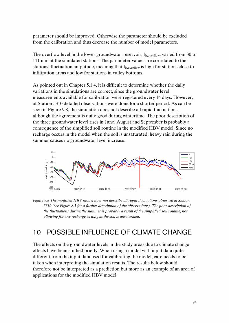
94

parameter should be improved. Otherwise the parameter should be excluded from the calibration and thus decrease the number of model parameters. The overflow level in the lower groundwater reservoir, llz,overflow, varied from 30 to 111 mm at the simulated stations. The parameter values are correlated to the stations' fluctuation amplitude, meaning that llz,overflow is high for stations close to infiltration areas and low for stations in valley bottoms. As pointed out in Chapter 5.1.4, it is difficult to determine whether the daily variations in the simulations are correct, since the groundwater level measurements available for calibration were registered every 14 days. However, at Station 5310 detailed observations were done for a shorter period. As can be seen in Figure 9.8, the simulation does not describe all rapid fluctuations, although the agreement is quite good during wintertime. The poor description of the three groundwater level rises in June, August and September is probably a consequence of the simplified soil routine in the modified HBV model. Since no recharge occurs in the model when the soil is unsaturated, heavy rain during the summer causes no groundwater level increase.

2007-04-26 2007-07-15 2007-10-03 2007-12-22 2008-03-11 2008-05-30-120

-100

-80

-60

-40

-20

0

20

Leve

l [cm

rel

. to

g.l.

]

H1

H2

H35310

HBV

Figure 9.8 The modified HBV model does not describe all rapid fluctuations observed at Station

5310 (see Figure 8.5 for a further description of the observations). The poor description of the fluctuations during the summer is probably a result of the simplified soil routine, not allowing for any recharge as long as the soil is unsaturated.

10 POSSIBLE INFLUENCE OF CLIMATE CHANGE

The effects on the groundwater levels in the study areas due to climate change effects have been studied briefly. When using a model with input data quite different from the input data used for calibrating the model, care needs to be taken when interpreting the simulation results. The results below should therefore not be interpreted as a prediction but more as an example of an area of applications for the modified HBV model.

95

The input data used is precipitation and temperature from climate simulations carried out at Rossby Centre, SMHI (see Figure 10.1). These series are output data from simulations using the regional model RCA3, which in turn uses data from the global model Echam5A, where A stands for a certain set of starting conditions. The emission scenario used is SRES A1b.

1982 2009 2036 2064 2091Year

0

4

8

12

16

Yea

rly m

ean

tem

pera

ture

[o C]

Temperature [oC]Precipitation [mm/day]

0

1

2

3

4

Yea

rly m

ean

prec

ipita

tion

[mm

/day

]

Figure 10.1 Climate simulations of precipitation and temperature, used as input in the modified

HBV model.

Simulations were made for Stations 5208 and 5213 in Sandsjöbacka. Groundwater levels were simulated from 1961 to 2100 and the simulated levels for the period 2075-208024 were compared with groundwater level observations from the period 1975-1980. As seen from Figure 10.2, the simulations indicate groundwater level fluctuations in the same order of magnitude as the observed levels.

24 For Station 5313 the period 2073-2078 was used.

96

Figure 10.2 Groundwater level simulations with input data from Figure 10.1. Upper: simulation of

Station 5208 for the period 2075-2080 is compared with observations for the period 1975-1980; Lower: simulation of Station 5213 for the period 2073-2078 is compared with observations for the period 1973-1978.

The reason for the simulated groundwater levels to be as similar to the observed levels as seen in Figure 10.2 can be found by analysing the water balance in the model. Since the input data changes over time, as shown in Figure 10.1, a corresponding change must be seen somewhere inside the model. In Figure 10.3, the recharge into the upper groundwater reservoir is illustrated. However, this appears to be generally unchanged over time.

1965 1975 1985 1995 2065 2075 2085 2095Year

0

10

20

30

40

Rec

harg

e [m

m/d

ay]

Figure 10.3 Simulation of recharge for Station 5208 in the modified HBV model, together with a

running 31-day average. The recharge is indicated with cyan and red for the two periods in the 20th and the 21st century respectively, and the running average is shown in black.

2073 2075 2076 2077

-200

-100

0

100

200

Leve

l rel

. to

g.l.

[cm

]

2075 2076 2077 2079 2080

-200

-100

0

100

200Le

vel r

el. t

o g.

l. [c

m]

97

Consequently, the increased precipitation has disappeared before it reaches the groundwater reservoirs. The explanation for this is increased evapotranspiration due to the increase in temperature, as seen in Figure 10.4.

1965 1975 1985 1995 2065 2075 2085 2095Year

0

2

4

6

Eva

potr

ansp

iratio

n [m

m/d

ay]

Figure 10.4 Simulation of evapotranspiration for Station 5208 with the modified HBV model,

together with a running yearly average. The evapotranspiration is indicated with cyan and red for the two periods in the 20th and the 21st century respectively, and the running average is shown in black.

Whether this high increase in evapotranspiration is correct has not been investigated further. However, it can be noted that the soil routine in the modified HBV model requires the soil moisture to be equal to the field capacity for recharge to occur. Consequently, precipitation during the summer to a large extent causes evapotranspiration rather than recharge. To illustrate the effect of decreased evapotranspiration, test simulations with a 50% decrease in the potential evapotranspiration were made. During certain summers there is a substantial increase in the groundwater levels due to decreased actual evapotranspiration, although during the winters the difference in evapotranspiration is smaller and the change in groundwater level is low (see Figure 10.5).

98

Figure 10.5 Simulations of Station 5208 with potential evapotranspiration, EP, decreased by 50%.

The original simulations are indicated with cyan and red for the two periods in the 20th and the 21st century respectively, while the simulations with reduced evapotranspiration are shown in black. Upper: the groundwater levels are raised substantially in relation to the original simulation during certain summers; Lower: the actual evapotranspiration is lowered substantially during certain summer periods in relation to the original simulations.

The small difference in groundwater levels during winter, due to the decreased evapotranspiration, suggests that the model overflows limit the maximum levels. To test this, a highly fictive simulation with a 50% increase in the precipitation, but with the original potential evapotranspiration, was carried out. As seen from Figure 10.6, this simulation indicates slightly higher groundwater level increases during the winter than in Figure 10.5. However, the increase in the level is still small due to a large increase in overflow from the lower groundwater reservoir.

1975 1977 1979 2075 2077 2079Year

-40

0

40

80

120

160

Leve

l [cm

rel

. to

g.l.]

1975 1977 1979 2075 2077 2079Year

0

1

2

3

4

5

Eva

potr

ansp

iratio

n [m

m/d

ay]

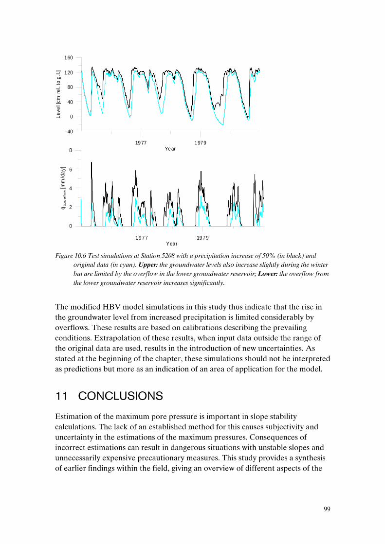
99

Figure 10.6 Test simulations at Station 5208 with a precipitation increase of 50% (in black) and

original data (in cyan). Upper: the groundwater levels also increase slightly during the winter but are limited by the overflow in the lower groundwater reservoir; Lower: the overflow from the lower groundwater reservoir increases significantly.

The modified HBV model simulations in this study thus indicate that the rise in the groundwater level from increased precipitation is limited considerably by overflows. These results are based on calibrations describing the prevailing conditions. Extrapolation of these results, when input data outside the range of the original data are used, results in the introduction of new uncertainties. As stated at the beginning of the chapter, these simulations should not be interpreted as predictions but more as an indication of an area of application for the model.

11 CONCLUSIONS

Estimation of the maximum pore pressure is important in slope stability calculations. The lack of an established method for this causes subjectivity and uncertainty in the estimations of the maximum pressures. Consequences of incorrect estimations can result in dangerous situations with unstable slopes and unnecessarily expensive precautionary measures. This study provides a synthesis of earlier findings within the field, giving an overview of different aspects of the

1977 1979Year

-40

0

40

80

120

160L

eve

l [cm

rel

. to

g.l.

]

1977 1979Year

0

2

4

6

8

qlz

,ov

erflo

w [

mm

/da

y]

100

problem. The groundwater levels in confined aquifers in three study areas along the Swedish west coast have been analysed with regard to pressure levels and fluctuations. The main aim of this study was to increase the understanding of distribution and fluctuation patterns in groundwater levels in confined aquifers and also to find objective physical and geological criteria governing the observed fluctuation patterns. Even though the research revealed weaknesses in the investigation method many new problems have been brought to light and the main objectives were accomplished. Studies of water level fluctuations in the Swedish Groundwater Network have indicated different fluctuation patterns, which have also been confirmed by simulations. These patterns are related to infiltration areas, downstream conditions and position within an aquifer. The simulations were mainly carried out using a slightly modified version of the hydrological HBV model. The model description in the modified HBV model is highly conceptual and can be criticised for oversimplifying the actual processes. Nevertheless, the model can simulate the observed groundwater level fluctuations satisfactorily. In addition, validation simulations showed that even with little hydrogeological information of an area, the groundwater levels can be simulated reasonably correctly. When applying a model in an area quite different from what the model was designed for, care must be taken when interpreting the results. The initial aim was to validate the results, using the FEM software SEEP, by comparing the modified HBV modelling results with results from a more detailed model. However, this aim was not achieved entirely and only simple parameter studies using SEEP were carried out. In addition to simulations of the prevailing climate situation, test simulations with input data series considering climate change were also made. These simulations indicate that the overflows in the confined aquifers have a strong limiting effect on the maximum groundwater levels. However, in these simulations the model is applied to input data outside the range of the input data used in the calibrations, which introduces new uncertainties. These simulations have not been analysed thoroughly and no definite conclusions should be drawn from the presented results. Brief analyses of the Chalmers model have also revealed the importance of the Swedish Groundwater Network. Particularly important properties are the

101

distances between observation areas, measurement frequency and data quality. Quality problems encountered included obviously erroneous observations and silted-up filters with decreased permeability. The correctness of the predictions, using the Chalmers model, was found to be highly dependent on the quality of the Groundwater network observations.

11.1 Practical implications Using the modified HBV model, groundwater level fluctuations, and maximum groundwater levels, can be simulated in areas, also where the hydrogeological knowledge is little. Since the knowledge of hydrogeological parameters almost always is rather limited, the usage of the modified HBV model can be a useful tool. An advantage with the model is that the relatively well known input data of precipitation and temperature is used. In addition to applications regarding prediction of future groundwater situations, the model can be used to simulate historical fluctuations, e.g. for the purpose of calculating groundwater level return-periods. Based on results and conclusions presented in the study, some simple recommendations for handling of pore pressure estimation in slope stability calculations can be given. The recommendations, aimed at not requiring advanced modelling, can also be seen as a result of the experience from the working process.

- Prioritise. Find out whether the stability of the specific slope is sensitive to changes in pore pressure before detailed measurements and investigations are carried out. If the stability is unaffected by pore pressure levels higher than what can be reasonably expected, i.e. the undrained shear strength governs the strength of the soil, no further pore pressure investigations are necessary. On the contrary, if the pore pressures affect the slope stability then extended investigations are necessary.

- Try to acquire a general understanding of the groundwater situation in an area slightly larger than the one where the specific stability problem is located. This analysis could, for example, result in a simple model for how water flow occurs in the confined aquifer as well as in the clay, together with estimations of the highest possible pressure level for the area, determined from overflow levels.

- Bear in mind that possible friction material layers within the clay can be connected to a deeper confined aquifer and thus have the same pressure level as in the confined aquifer. A high pressure level in the confined aquifer has a greater effect on the pore pressure in clay when the clay

102

thickness is small. This means that an area where the clay thickness is for some reason thinner than is generally the case, the risk of high pore pressures is increased.

- Relate observed groundwater and pore pressure levels to the seasonal groundwater levels by considering the time of the year for the observations together with the general yearly fluctuations for the specific climate region. Even better is to relate the observations to the present groundwater situation for the region, which can be received e.g. from SGU. The position within the present aquifer should also be considered and it should be taken into account that the pressure variations are larger close to infiltration areas than in valley bottoms.

- Consider that for shallow slip surfaces the groundwater level in the upper aquifer can be of greater importance than the pressure level in the confined aquifer.

- When applying the Chalmers model, use several reference stations and put highest weight to the prediction results from reference stations in similar aquifer positions as the prediction station. Moreover, be observant of the data quality in the Groundwater Network.

11.2 Future work Several areas for future work related to estimation of maximum pore pressures have been identified. One obviously important part is to identify better under what conditions the estimation of maximum pore pressure is important, i.e. when the drained shear strength governs the soil strength. Presumably, research in this area will need to focus more on the upper aquifer than has been done in this study. More research on the effect from friction material layers inside the clay is also needed. To increase the knowledge of groundwater level fluctuations with regard to local geological conditions, extended synthesis and classification of groundwater level and pore pressure data could be made in a manner similar to what has been done in this study. Groundwater level and pore pressure measurements are carried out within numerous projects, primarily construction work but also in slope stability investigations. However, a synthesis of this large number of measurements has never been made. The modified HBV model can be developed further, e.g. by improving the soil routine and the overflow in the lower groundwater reservoir. A more physically correct model description than in the modified HBV model's response function

103

could probably improve the identification of significant physical parameters governing the groundwater fluctuation patterns. Moreover, the climate change simulations could be improved through more detailed analyses and tests. The Chalmers model has considerable potential but also considerable scope for improvement, indicating that continued testing and development is necessary. Improvements can be based on the findings in this study of fundamental differences in fluctuation pattern. The possibility of using the Chalmers model together with the HBV model would also be interesting to investigate. Extended studies of the effects of climate change could be done also with the Chalmers model.

104

12 REFERENCES

Alén, C. (1998). On probability in geotechnics. Gothenburg, Chalmers Technical

University. PhD. Andréasson, J., S. Bergström, et al. (2004). "Hydrological Change –

Climate Change Impact Simulations for Sweden." AMBIO: A Journal of the Human Environment 33(4): 228-234.

BAT. (2008). "BAT - Groundwater Monitoring System." Retrieved 2008-11-17, from http://www.bat-gms.com/.

Bengtsson, J. and J. Boström (2008). Prognostisering av höga grundvattennivåer med Chalmersmodellen. Civil and environmental engineering. Göteborg, Chalmers Technical University. Master.

Bergdahl, U. and M. Tremblay (1987). Pore pressure measurements as a means of slope stability monitoring. Dublin.

Bergström, S. (1976). Development and application of a conceptual runoff model for Scandinavian catchments. SMHI Reports RHO, No. 7. Norrköping, Sweden.

Bergström, S. (1990). Parametervärden för HBV-modellen i Sverige. SMHI Hydrologi. Nr. 28. Norrköping, Sveriges Metereologiska och Hydrologiska Institut.

Bergström, S. and G. Sandberg (1983). "Simulations of Groundwater Response by Conceptual Models – Tree Case Studies." Nordic Hydrology 14(2): 71-84.

Berntsson, J. A. (1983). Portrycksvariationer i leror i Göteborgsregionen. Institutionen för Geoteknik med grundläggning. Göteborg, Chalmers Tekniska Högskola. PhD.

Bockgård, N. (2004). Groundwater Recharge in Chystalline Bedrock. Processes, Estimation and Modelling. Department of Earth sciences. Uppsala, Uppsala University. PhD.

Buma, J. (2000). "Finding the most suitable slope stability model for the assessment of the impact of climate change on a landslide in southeast France." Earth Surface Processes and Landforms 25(6): 565-82.

Cato, J. and M. Engdahl (1982). Inventering av lutande lermark. SGU Meddelande nr 20. Uppsala.

Chow, V. T., D. R. Maidment, et al. (1988). Applied Hydrology, McGraw-Hill. Colleuille, H., S. Beldring, et al. (2006). Groundwater and Soil Water System for

Norway based on daily simulations and real-time observations. International Symposium Dijon. IAH France.

CoSS (1995). Commission on Slope Stability. K. Axelsson, P.-E. Bengtsson, P. Engströmet al. Sweden, Royal Swedish Academy of Engineering Science.

Crosta, G. B. (2004). "Introduction to the special issue on rainfall-triggered landslides and debris flows." Engineering Geology 73(3-4): 191-192.

105

Crosta, G. B. and P. Frattini (2008). Rainfall-induced landslides and debris flows. Hydrological processes. 22: 473-477.

Dehn, M., G. Buerger, et al. (2000). "Impact of climate change on slope stability using expanded downscaling." Engineering Geology 55(3): 193-204.

Fetter, C. W. (1994). Applied hydrogeology. New Jersey, Prentice-Hall, Inc. Freeze, A. R. and J. A. Cherry (1979). Groundwater. Englewood Cliffs, Prentice-

Hall. GEO-SLOPE (2008). Seepage Modeling with SEEP/W 2007 - An Engineering

Methodology. Guzzetti, F. (1998). "Hydrological triggers of diffused landsliding."

Environmental Geology 35(2): 79-80. Guzzetti, F., S. Peruccacci, et al. (2005). Definition of critical threshold for

different scenarios. RISK AWARE. RISK-Advanced Weather forecast system to Advise on Risk Events and management. Perugia, Italy.

Hansbo, S. (1960). Consolidation of clay, with special reference to influence of vertical sand drains. A study made in connection with full-scale investigations at Skå-Edeby. Gothenburg, Sweden, Chalmers Technical University.

Hartlén, J., C. Alén, et al. (2007). "Skredet i Småröd december 2006." from www.vv.se.

Huisman, L. (1972). Groundwater Recovery. London and Basingstoke, MACMILLAN.

Hultén, C., M. Olsson, et al. (2005). Släntstabilitet i jord - Underlag för handlingsplan för att förutse och förebygga naturolyckor i Sverige vid förändrat klimat. Linköping.

Häggström, S. (1988). Hydraulik för V-teknologer. Göteborg, Department of Hydraulics, Chalmers University of Technology.

Johansson, B. (2002). Estimation of areal precipitation for hydrological modelling in Sweden. Earth Sciences Centre, Department of Physical Geography. Göteborg, Göteborg University.

Johansson, Å. (2006). Personal communication. Authority examiner of geotechnical investigations in Sweden, Swedish Geotechnical Institute.

Johnson, J. (1993). Utveckling av metodik för simulering och prognos av grundvattennivåer. Uppsala, SGU.

Knutsson, G. and T. Fagerlind (1977). Grundvattentillgångar i Sverige. SGU Rapporter och meddelanden, nr. 9. Uppsala, Sveriges Geologiska Undersökning.

Kruseman, G. P. and N. A. de Riddler (1970). Analysis and evaluation of pumping test data. Wageningen, Netherlands.

Larsson, R. (1986). Consolidation of soft soils. SGI Report No. 29. Linköping. Larsson, R. and H. Åhnberg (2003). Long-term effects of excavations at crests of

slopes. Report. Linköping. Lindström, G., K. Bishop, et al. (2002). "Soil frost and runoff at Svartberget,

northern Sweden – measurement and model analyses. ." Hydrological processes 16: 3379-3393.

106

Lindström, G., J. Rosberg, et al. (2005). "Parameter Precision in the HBV-NP Model and Impacts on Nitrogen Scenario Simulations in the Rönneå River, Southern Sweden." AMBIO: A Journal of the Human Environment 34(7).

Malet, J. P., T. W. J. van Asch, et al. (2005). "Forecasting the behaviour of complex landslides with a spatially distributed hydrological model." Nat. Hazards Earth Syst. Sci. 5(1): 71-85.

McInnes, R., J. Jakeways, et al. (2007). Landslides and Climate Change. Landslides and Climate Change, Isle of Wight, Taylor & Francis.

Pearson, E. S. and H. O. Hartley (1972). Biometric tables for statisticans. Vol II. Cambridge, Cambridge University Press.

Persson, J. (2007). Hydrogeological Methods in Geotechnical Engineering. Civil and Environmental Engineering. Göteborg, Chalmers Technical University. PhD.

Ramli, M., Y. Ohnishi, et al. (2007). "Coupled tank model and flow model for slope seepage flow analyses." Journal of the Southeast Asian geotechnical society August.

Rodhe, A., G. Lindström, et al. (2006). Grundvattenbildning i svenska typjordar - översiktlig beräkning med en vattenbalansmodell. Uppsala, Department of Earth Sciences - Hydrology, Uppsala University.

Rosén, B. (1991). Prognoser av grundvattennivåer/portryck – Etapp 1: Jämförande beräkningsexempel med Lathunden och HBV-modellen. Linköping, Sweden, Swedish Geotechnical Institute.

Rossby Centre, S. (2007). "Sveriges klimat i framtiden." Retrieved September 2nd, 2008, from http://www.smhi.se/sgn0106/leveranser/sverigeanalysen/.

Sandberg, G. (1982). Utvärdering och modellsimulering av grundvattenmätningarna i Ångermanälvens övre tillrinningsområde. Hydrologiska/Oceanografiska avdelningen, SMHI. Norrköping, Sweden.

Seibert, J., K. H. Bishop, et al. (1997). "Test of TOPMODEL's ability to predict spatially distributed groundwater levels." Hydrological Processes 11(9): 1131-1144.

SGU (1985). Svenskt vattenarkiv - Grundvattennätet. SGU Rapporter och meddelanden nr 43. Uppsala.

SMHI. (2008). "The HBV model." Retrieved September 5th, 2008, from http://www.smhi.se/sgn0106/if/hydrologi/hbv.htm.

SRV. (2008). "Var inträffar skred och ras?" Retrieved 2008-12-10, from www.raddningsverket.se.

Svensson, C. (1984). Analys och användning av grundvattennivåobservationer. Geologi. Göteborg, Chalmers tekniska högskola / Göteborgs universitet. PhD.

Svensson, C. and G. Sällfors (1985). Beräkning av dimensionerande grundvattentryck - 1. Göteborgsregionen. Beräkning av dimensionerande grundvattentryck. Göteborg, Geologi / Geoteknik med grundläggning.

Sällfors, G. (1986). Slänters stabilitet. Göteborg, Institutionen för geoteknik med grundläggning, Chalmers Tekniska Högskola.

Sällfors, G. (2001). Geoteknik. Göteborg, Chalmers Technical University.

107

Terlien, M. T. J. (1998). "The determination of statistical and deterministic hydrological landslide-triggering thresholds." Environmental Geology 35(2-3).

Terzaghi, K., R. B. Peck, et al. (1996). Soil Mechancs in Engineering Practice. New York, John Wiley & Sons, Inc.

Thorsbrink, M. and B. Thunholm (2004). Utvärdering och utveckling av Grundvattennätets nivådata. Uppsala.

Thunholm, B. (2008). Personal communication. Groundwater level variations in different regions of Sweden, Sveriges Geologiska Undersökning.

Todd, D. K. (1959). Ground Water Hydrology. New York, John Wiley & Sons, Inc.

Tremblay, M. (1990). Mätning av grundvattennivå och portryck. SGI Information. Linköping.

Wikipedia, t. f. e. (2008). "Debris flow." Retrieved 2 September, 2008, from http://en.wikipedia.org/wiki/Debris_flow.

!!

!!

!!

!!

!!

!!

!!

!

!!

!!

!!

!!

!!

!!!

!!!

!

!!

!

!!!!!!

!!

!!

!!!

!!

!!

!!

!!

!!

!

!

!!

!!

!

!!

!!

!!

!!

!!

!!

!!

! ! ! !!

!! !

! ! !!

!

!!

!!

!!

!!

!!

!!

!!

!! ! ! ! ! ! ! ! ! ! ! ! ! ! ! !

!!

!!

!!

!!

!!

!

!!

!!

!!

!

!!

!!

!!

!!

!!

!!

!

!!

!

!! !

! ! ! ! ! ! !!

!!

!!

!

!!

!!

!!

!!

!

!!

!!

!!

!!!!

!

!!

!!

!!

!!

!!

!!

!!

!!

!!

!!

!!

!!

!!

!!

!!

!!

!!

!!

!!

!!

!!

!!

!!

!!

!!

!!

!!

!!

!!

!!

!!

!!

!!

!!

!!

!!

!!

!

!!

!!

!!

!!

! ! ! ! ! ! ! ! ! ! ! ! ! !!

!

!!

!!

!!

!!

!!

!

!!

!!!!!

!!

!!

!!!!!

!!

!!!

!!

!!!!!!!!!!!!

!!

!!

!!!

!!

!!!

!!

!!

!!!!

!!

!!

!!

!

!!

!!

!!

!

!!

!!

!!

!!

!!

!!!!!!!!

!!

!!

!!

!

!!

!!

!!

!!

!! ! ! ! ! ! ! ! ! !

! ! ! ! ! ! !! !

!!

!!

!!

!!

! ! ! !!

!!

!!!

!!!

!!

!!

!

!!

!

!!

!!

!!

!!

!!

!

!!!

!!

!!

!!

!

!!

!!

!!

!!

!!

!!

!

!!

!!

!!

!!

!!

!!

!!

!!

!!

!!

!!

!!

!!

!!

!!

!!

!!

!!

!!

!!

!!

!!

!!

!

!!

!!!!!!!!!!

!!

!!

!!!!!!!!!!

!!

!!

!!

!!

!!

!!

!!

!!

!!!

!!!!!!!!!!!!

!!!!!!

!!

!!

!!

!!

!!

!!

!!

!!

!!

!!

!!

!!

!!

!!

!!

!!

!!

!!

!!

!!

!!

!!

!!

!!!

!!

!

!!

!!

!!

!!

!

! ! !

!

!!

!!

!!

!!

!!

!!!

!!

!!

!!

!!

!!

!!

!!

!!

!!

!

!!

!!

!!

!!

!!

!!!

!

!!!! !

!

!!

!!

!!

!!

!!

!!

!!

!!

!!

!!!

!!

!!

!!

!!!!

!!

!!

!!

!!

!!

!!

!

!!

!!!!!!!

!!!!!!!

!!!!!!

!!

!!

!!

!!

!!

!!

!!

!!

!!

!!

!!

!!

!!

!!!!!!!

!!!

!!

!!

!!

!!

!!

!!!

!

!

!

!

!

!

!

!

!

!

!

!

!

!

!

!

!

!

!

!

!

!

!

!

!

!

!

!

!

!!

!

!

!

!

!

!

!

!

!!

!

!

!!

!

!

!

!

!

!

!

!

!

!

!

!

!

!

!

!

!

!

!

!

!

!

!

!!

!!

!!

!

!

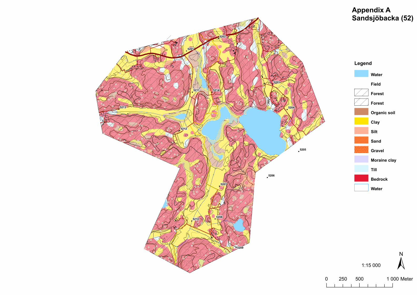
50

75

100

75

75

75

75

75

75

75

50

100

75

50

50

100

50

50

75

100

75

75

50

50

75

75

100

75

75

75

100

50

75

75

75

75

75

50

50

75

50

100

75

75

75

50

75

75

75

75

75

75

75

75

75

50

75

100

4555

60

65

70

80

85

90

95

40

65

65

90

55

85

95

55

70

55

80

65

95

90

55

55

60

80

65

55

80

95

90

65

80 70

65

85

70

80

65

60

90

55

85

5580

95

80

65

85

6590

55

65

85

90

90

55

85

6585

85

80

70

85

70

80

95

65

95

85

60

70

85

90

65

65

95

90

80

60

65

90

80

80

70

9585

80

70

70

45

60

80

85

85

65

55

95

70

45

65

60

45

70

80

60

85

60

80

80

70

60

70

85

55

85

55

90

70

85

90

85

60

60

95

70

7065

85

95

80

95

85

70

90

80

70

80

60

40

80

90

80

80

65

85

60

80

90

55

70

90

60

85

90

80

90

70

55

70

70

55

65

85

70

45

85

60

90

85

60

85

90

90

70

80

80

70

80

60

85

65

60

80

80

70

70

95

95

95

95

95

80

80

90

70

55

85

90

70

4585

60

65

80

85

80

60

60

65

85

60

85

80

80

85

80

65

70

70

90

60

80

85

90

85

80

90

55

65

85

90

80

9070

90

40

70

65

90

65

60

65

45

65

80

65

5214

5213

5212

5211

5210

5209

5208

5207

5206

5205

5204

5203

5202

5201

0 500 1 000250 Meter±1:15 000

Appendix ASandsjöbacka (52)

LegendWaterFieldForestForestOrganic soilClaySiltSandGravelMoraine clayTillBedrockWater

!

!

!

!

!

!

!

!

!

!

!

!

!

!

!

!

!

!

!

!

!

!

!

!

!

!

!

!

!

!

!

!

!

!

!

!

!

!

!

!

!

!

!

!

!

!

!

!

!

!

!

!

!

!

!

!

!

!

!

!

!

!

!

!

!

!

!

!

!

!

!

!

!

!

!

!

!

!

!

!

!

!

!

!! !

!

!

!

!

!

!

!

!

!

!

!

!

!

!

!

!

!

!

!

!

!

!

!

!

!

!

!

!

!

!

!

!

!

!

!

!

!

!

!

!

!

!

!

!

!

!

!

!

!

!

!

!

!

!

!

!

!

!

!

!

!

!!

!

!

!

!

!

!

!

!

!

!

!

!!

!!

!

!

!

!

!

!

!

!

!

!

!

!

!

!

!

!

!

!

!

!

!

!

!

!

!

!

!

!!

!

!

!

!

!

!

!

!

!

!

!

!

!

!

!

!

!

!

!

!

!

!

!

!

!

!

!

!

!

!

!

!

!

!

!

!

!

!

!

!

!

!

!

!

!

!

!

!

!

!

!

!

!

!

!

!

!

!

!

!

!

!

!

!

!

!

!

!

!

!

!

!

!

!

!

!

!

!

!

!

!

!

!

!

!

!

!

!

!

!

!

!

!

!

!

!

!

!

!

!

!

!

!

!

!

!

!

!!

!!

!

!

!

!

!

!

!

!

!

!

!

!

!

!

!!

!

!

!

!

!

!

!

!

!

!

!

!

!

!

!

!

!

!

!

!

!

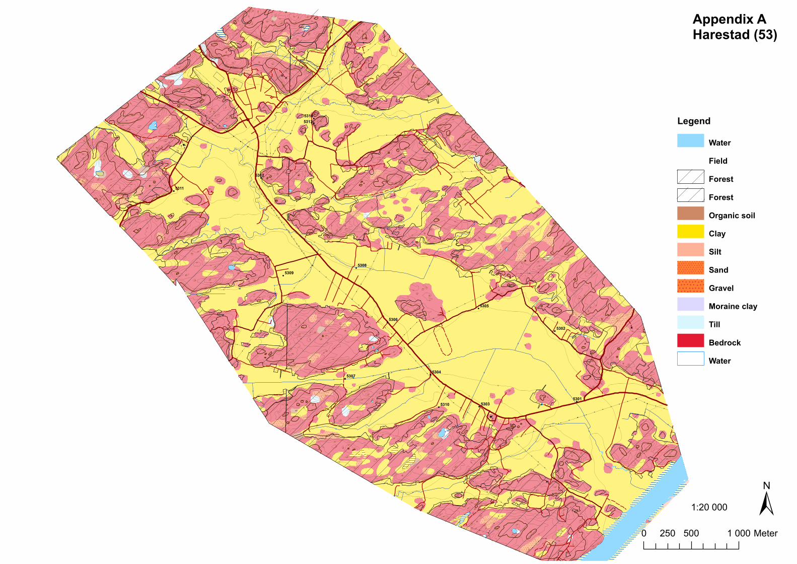
25

50

75

25

25

75

25

50

50

75

50

25

25

25

50

25

50

50

50

75

25

25

25

50

25

25

50

50

25

25

25

25

50

25

25

25

25

50

50

50

25

75

25

50

25

25

25

25

50

50

50

50

25

50 50

50

50

75

25

50

5050

25

50

25

25

25

25

25

50

75

25

75

25

50

50

75

50

25

25

25

50

25

25

25

25

25

25

25

50

25

50

50

50

50

25

25

25

50

50

50

25

25

25

50

25

50

50

25

25

50

25

50

50

50

25

75

50

50

50

25

25

25

25

25

50

25

25

25

25

25

50

50

50

25

50

75

50

50

75

50

50

5025

50

50

25

25

25

50

50

25

50

50

25

25

50

25

25

25

50

25

25

50

25

25

25

25

50

5025

25

50

25

25

50

25

50

50

15

10

20

30

5

45

35

55

40

60 65

70

80

85

25

50

90

35

45

55

35

55

40

30

20

40

45

40

30

40

4040

80

20

40

45

70

60

20

45

60

10

35

60

45

40

60

35

45

40

40

60

40

35

70

60

60

40

45

30

45

30

45

45

35

45

35

40

40

35

40

15

20

30

20

30

45

55

20

40

45

20

30

35

70

40

40

45

45

50

20

15

45

30

35

40

45

65

30

70

35

60

40

40

35

30

55

30

40

40

45

30

65

35

30

20

40

15

45

15

35

60

15

20

45

15

30

35

55

40

35

45

15

30

35

35

30

35

20

45

15

80

35

35

55

65

40

35

40

35

55

45

40

20

45

80

40

35

30

45

45

40

15

40

35

35

30

35

45

30

45

30

20

30

40

30

55

45

45

30

45

4055

35

40

30

35

40

45

35

35

45

40

40

60

55

45

45

55

40

40

40

45

55

35

30

45

45

85

30

35

60

35

45

55

45

20

35

35

30

40

65

35

35

20

40

40

15

45

15

25

35

20

50

65

35

80

30

20

70

45

45

40

40

55

55

70

45

45

55

20

20

35

70

45

55

40

35

20

45

30

85

55

40

35

35

35

35

35

40

35

35

70

80

4065

60

35

30

20

35

20

55

40

35

45

45

35

60

40

10

45

55

20

40

45

80

45

40

40

30

70

30

35

35

35

55

45

20

45

35

80

35

20

30

15

40

45

40

45

35

10

65

15

45

45

30

15

40

45

35

60

20

40

30

40

45

70

45

30

55

40

50

15

45

30

45

40

20

30

10

40

40

10

40

40

40 35

40

40

35

45

55

35

3035

15

45

35

60

45

3535

5

40

60

40

10

30

35

45

15

60

50

30

35

35

45

65

20

45

65

30

45

55

35

30

55

65

30

5545

30

30

40

30

35

15

30

65

45

80

20

40

20

40

45

50

30

35

30

35

40

30

50

55

50

15

35

60

15

40

30

20

15

55

35

30

35

45

35

40

80

85

40

70

40

30

40

40

40

30

70

40

30

45

45

55

70

55

45

20

45

65

40

40

70

20

20

30

35

30

35

70

30

35

40

80

55

45

20

35

60

65

35

30

40

30

45

60

40

30

35

35

45

70

90

65

35

35

45

55

20

45

30

40

65

40

60

65

40

70

35

15

30

20

40

5

20

35

40

30

40

45

40

55

35

4520

60

30

4530

20

15

15

45

35

65

45

40

55

15

20

30

70

40

35

35

15

30

30

40

20

45

45

65

30

35

30

45

45

40

30

35

45

40

20

40

35

10

55

40

30

30

45

20

35

85

20

45

30

45

80

40

45

40

20

55

55

30

40

40

60

40

30

15

20

35

55

35

45

40

20

45

85

30

35

30

40

45

45

10

40

60

45

30

35

30

45

30

5

40

35

45

20

65

35

45

15

35

40

45

30

40

45

55

53145313

5312

5311

5310

53095308

5307

5306

5305

5304

5303

5302

5301

0 500 1 000250 Meter±1:20 000

Appendix AHarestad (53)

LegendWaterFieldForestForestOrganic soilClaySiltSandGravelMoraine clayTillBedrockWater

!!

!!

!!

!!

!!

!!

!

!!

!!

!!

!!

!!

!!

!!

!!

!!!!!!

!!

!

!!

!!

!

!!

!!

!!

!!!!!!

!!

!

!!

!

!!

!!

!!

!!

!!

!!

!!

!!

!!

!!

!!

!!

!

!!

!!!

!!!!

!!!!!!

!!

!!

!!

!!

!!

!!

!!

!!

!!!

!!

!!

!!

!!

!!

!!

!!

!!

!!

!!

!!

!!

!!

! ! !!

!

!!

!!

!

!!!!!!!!!!!!!!

!!

!!

!!

!!!

!!

!!

!!

!

!!

!!

!!

!!

!!

!!

!!!!!

!

!!

!

!!

!!

!!!

!!

!!

!!

!!

!

!!!

!!!

!!

!!

!!

!!!

!!

!!

!!!

!!

!!

!

!!

!

!!

!!

!!

!

!!

!!!

!! ! !

!!

!!

!!

!!

!!!!

!!

!!!

!!

!!

!!

!!

!!

!!!

!!

!!

!!

!!!

!!

!!

!

!!

!! ! !

!!

!!

!!

!!

!!

!!

!!

!

!!

!!

!!

!!

!!

!!

!!

!!

!!

!!

!!

!!

! !

!!

!!!

!!

!!

!

! ! ! ! ! ! ! ! !!

!!

!!

!!

!!

!!

!!

!!

!!

!!

!!

!!

!

!!

!

!!!

!!

!!

!!!

!!

!!

!!

!!

!!

!

!!

!!

!! ! ! ! ! ! ! ! !

!!

!!

!!

!!

!! ! ! ! ! ! ! ! !

!! ! !

!!

!!

!!

!!

!!

!!

!!

!!

!!

!!

!

!!

!!

!!

!!

!

!!

!!

!!

!!

!!!

!!

!!

!!

!!!

!!

!!

!!

!!

!

!!

!!

!!

!!

!!

!

!!!

!!

!!

!!

!!

!!!!!!!!!!

!!

!!!

!

!!

!!

!

!!

! ! ! !

!!

!!

!!!!

!!

!!!!!!

!!

!!

!!

!!

!!

!!

!!

!!

!

!!

!!

!!

!

!!

!!

!!

!

!!

!!

!!

!!

!!

!!

!!

!!

!

!!

!!!

!!

!!

!!

!!

!!

!!

!!

!

!!

!!

!

!!

!!

!!

!!

!!

!!!

!!!!

!

!!

! ! !!

!!

!! ! ! ! ! ! ! ! ! ! ! ! ! ! ! ! ! ! ! ! !

!!

!

! ! ! !

!!

!!

!

! ! ! !!

!!

!

!

!

!

!

!

!

!

!

!

!

!

!

!

!

!

!

!

!

!

!

!

!

!

!

!

!

!

!

!

!

!

!

!

!

!

!

!

!

!

!

!!

!

!!!

!

!

!

!

!!!!

!

!

!

!

!

!

!

!!

!!

!!

!

!

!

!

!

!

!

!

!

!

!

!

!

!

!

!

!

!

!

!

!

!

!

!

!

!

!

!

!

!

!

!

!

!

!

!

!

!

!

!

!

!

!!

!!

!

!

!

!

!

!

!

!

!

!

!

!

!

!

!

!

!

!

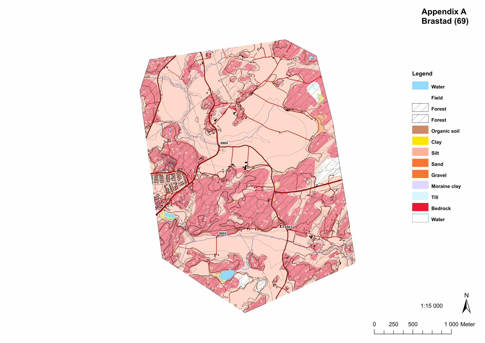
50

25

75

45

50

50

75

50

50

75

50

50

75

50

50

50

75

50

50

50

75

50

50

50

50

50 5050

25

50

5075

50

50

50

50

50

50

25

50

50

50

50

50

50

50

50

75

45

40

55

3560

30

65

70

50

80

55

60

55

60

30

60

60

65

45

70

45

70

55

70

55

55

55

60

70

60

55

65

60

65

65

65

65

60

70

55

65

55

70

55

60

70

60

55

55

45 70

55

60

65

60

55

60

40

70

60

55

70

65

55

65

70

70

55

70

40

70

40

60

80

55

45

55

60

60

60

65

40

45

40

55

55

60

60

55

65 55

40

6065

65

60

65

45

40

60

55

60

40

60

45

65

55

65

40

60

55

45

60

70

45

70

55

65

65

65

60

60

40

4045

55

60

45

55

65

80

60

60

60

70

65

55

45

60

55

65

60

60

55

60

60

60

65

60

45

55

65

65

65

60

40

70

70

60

60

65

60

60

45

65

55

65

45

65

60

55

45

70

70

60

60

70

4540

65

70

55

30

65

65

55

55

65

65

35

45

55

65

45

65

60

65

60

35

60

60

55

65

65

60

70

40

60

65

65

60

70

60

65

80

60

55

70

55

55

55

45

55

55

55

55

60

55

65

60

60

45

60

70

70

60

6904

69036902

0 500 1 000250 Meter±1:15 000

Appendix ABrastad (69)

LegendWaterFieldForestForestOrganic soilClaySiltSandGravelMoraine clayTillBedrockWater

Appendix B

Observations from field studies

Depth measurements from SGU (1985), Svensson (1984) and Bengtsson & Boström (2008). Active stations are displayed in bold.

Sandsjöbacka Harestad Brastad

Station Depth [m] (SGU)

Depth [m] (Svensson)

Depth [m] (Bengtsson & Boström)

Station Depth [m] (SGU)

Depth [m] (Svensson)

Depth [m] (Bengtsson & Boström)

Station Depth [m] (SGU)

Depth [m] (Svensson)

Depth [m] (Bengtsson & Boström)

5201 2 5301 23.3 24.2 6.87 6902 5.55 5.55

5202 5.8 6.1 5.74 5302 5.5 5.9 6903 5.5 5.45

5203 2.82 5303 13.75 4.75 6904 8.35 7.6

5204 2.1 2 5304 35.95

5205 9 3.4 5305 29.7 3.06

5206 1.9 5306 13.73

5207 13.4 14.4 5307 13.8 14.2 13.88

5208 13 13.7 9.77 5308 19.95

5209 7 7 6.08 5309 4.05 4.5

5210 18 18 5310 9.1 9.5 9.44

5211 15.8 15.5 5311 4.4 4.4 4.16

5212 4.1 4 5312 12.05

5213 7.55 7.5 7.17 5313 8.95 9.2

5214 7.45 8 5314 6.45

Transmissivity and time-lag measurements from SGU (2002 and 2005), Svensson (1984), SGI(2008) and Bengtsson & Boström (2008).

Active stations are displayed in bold.

Station Transmiss-

ivity [m2/s]

(Svensson)

Transmiss-

ivity [m2/s]

(Bengtsson

& Boström)

Transmiss-

ivity [m2/s]

(SGU)

Transmiss-

ivity [m2/s]

(SGI)

Time-lag

[min]

(Svensson)

Time-lag

[min]

(Bengtsson

& Boström)

Time-

lag

[min]

(SGU)

Time-

lag

[min]

(SGI)

5201

5202 2.00E-05 2.6·10-6 6.3 7.4

5203

5204

5205

5206

5207

5208 4.00E-06 9.0·10-8 2.3·10-8 9 216 855

5209 4.00E-06 5.3·10-6 5.4·10-6 10 3.6 3.6

5210

5211 5.8·10-8 332.2

5212

5213 8.00E-05 2.0·10-5 0.9 1

5214 1.00E-05 5.6·10-6 4 3.5

5301 4.7·10-7 3.9·10-7 41.1 50

5302

5303 2.2·10-9 7.1·10-9 ~0 8635 2716 infinite

5304

5305 1.8·10-9 ~0 ~0 10795 infinite infinite

5306 2.9·10-7 4.0·10-7 7.0·10-7 67.5 47.6 28

5307 4.5·10-9 4318

5308

5309

5310 4.5·10-8 6.4·10-8 3.1·10-8 431.8 300 617

5311 2.2·10-8 1.2·10-7 3.2·10-7 4.5 863.6 156 59

5312

5313 4

5314

6902 ~0 ~0 infinite infinite

6903 ~0 3·10-9 infinite 6378

6904 ~0 ~0 infinite infinite

Appendix C Pictures of groundwater stations

Station 5214

Station 5301

Groundwater station

Appendix D Typical screen dump from a calibration of the modified HBV model

Appendix E Calibration simulations

Sandsjöbacka

Apr-75 Aug-76 Jan-78 May-79 Oct-80

-200

-100

0

100

200

Leve

l rel

. to

g.l.

[cm

]

5208-cal

Apr-75 Aug-76 Jan-78 May-79 Oct-80

-200

-100

0

100

200

Leve

l rel

. to

g.l.

[cm

]

5209-cal

Apr-75 Aug-76 Jan-78 May-79 Oct-80

-200

-100

0

100

200

Leve

l rel

. to

g.l.

[cm

]

5211-cal

Dec-73 Apr-75 Aug-76 Jan-78

-200

-100

0

100

200

Leve

l rel

. to

g.l.

[cm

]

5213-cal

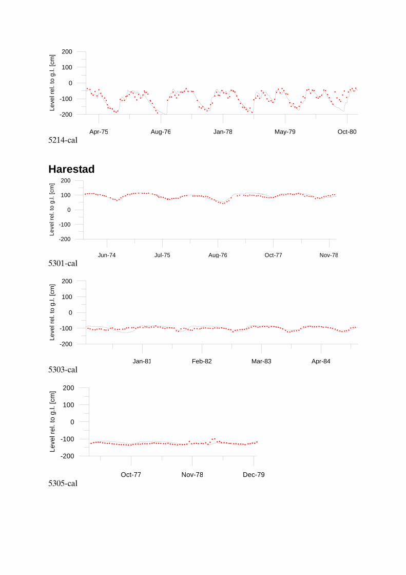
Apr-75 Aug-76 Jan-78 May-79 Oct-80

-200

-100

0

100

200Le

vel r

el. t

o g.

l. [c

m]

5214-cal

Harestad

Jun-74 Jul-75 Aug-76 Oct-77 Nov-78

-200

-100

0

100

200

Leve

l rel

. to

g.l.

[cm

]

5301-cal

Jan-81 Feb-82 Mar-83 Apr-84

-200

-100

0

100

200

Leve

l rel

. to

g.l.

[cm

]

5303-cal

Oct-77 Nov-78 Dec-79

-200

-100

0

100

200

Leve

l rel

. to

g.l.

[cm

]

5305-cal

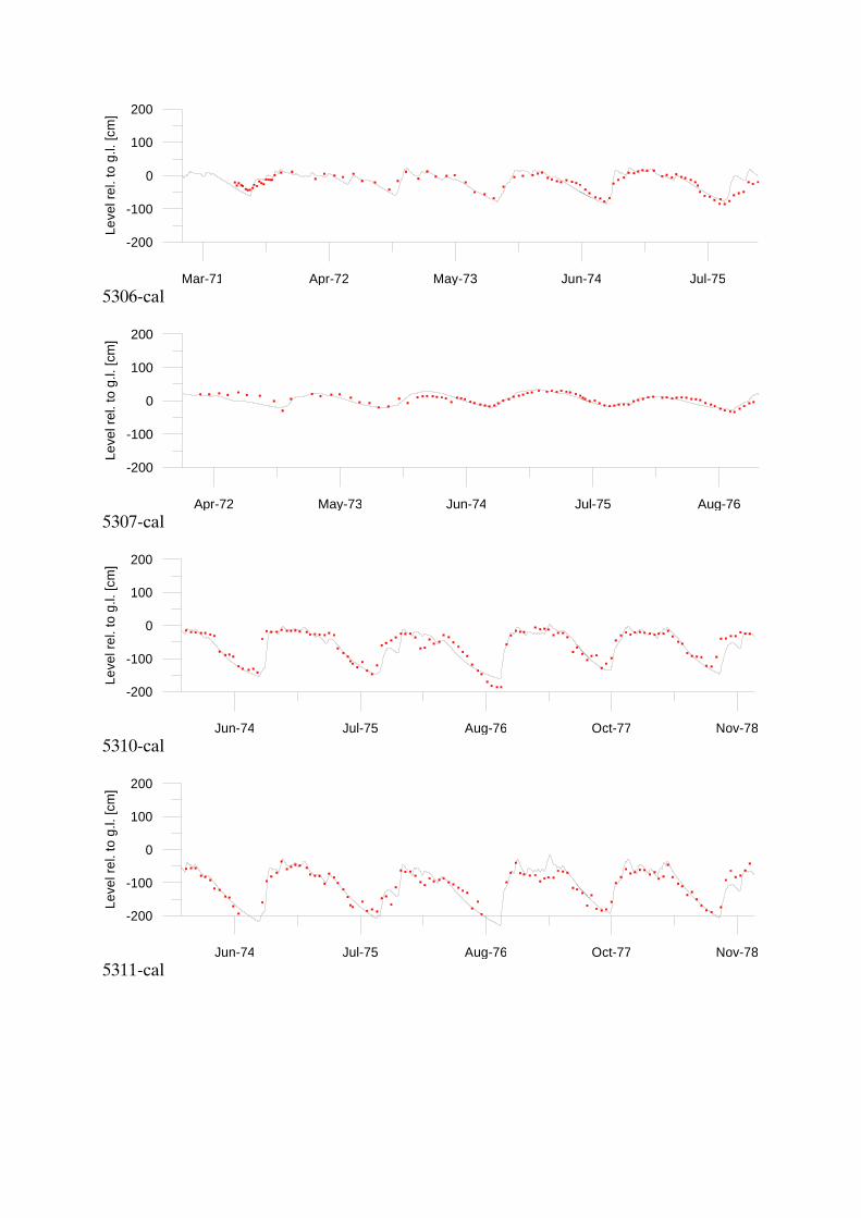
Mar-71 Apr-72 May-73 Jun-74 Jul-75

-200

-100

0

100

200Le

vel r

el. t

o g.

l. [c

m]

5306-cal

Apr-72 May-73 Jun-74 Jul-75 Aug-76

-200

-100

0

100

200

Leve

l rel

. to

g.l.

[cm

]

5307-cal

Jun-74 Jul-75 Aug-76 Oct-77 Nov-78

-200

-100

0

100

200

Leve

l rel

. to

g.l.

[cm

]

5310-cal

Jun-74 Jul-75 Aug-76 Oct-77 Nov-78

-200

-100

0

100

200

Leve

l rel

. to

g.l.

[cm

]

5311-cal

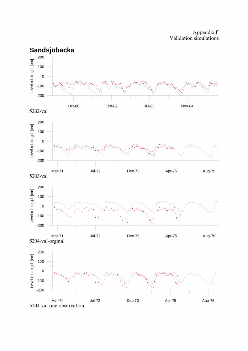
Appendix F Validation simulations

Sandsjöbacka

Oct-80 Feb-82 Jul-83 Nov-84

-200

-100

0

100

200

Leve

l rel

. to

g.l.

[cm

]

5202-val

Mar-71 Jul-72 Dec-73 Apr-75 Aug-76

-200

-100

0

100

200

Leve

l rel

. to

g.l.

[cm

]

5203-val

Mar-71 Jul-72 Dec-73 Apr-75 Aug-76

-200

-100

0

100

200

Leve

l rel

. to

g.l.

[cm

]

5204-val-orginal

Mar-71 Jul-72 Dec-73 Apr-75 Aug-76

-200

-100

0

100

200

Leve

l rel

. to

g.l.

[cm

]

5204-val-one observation

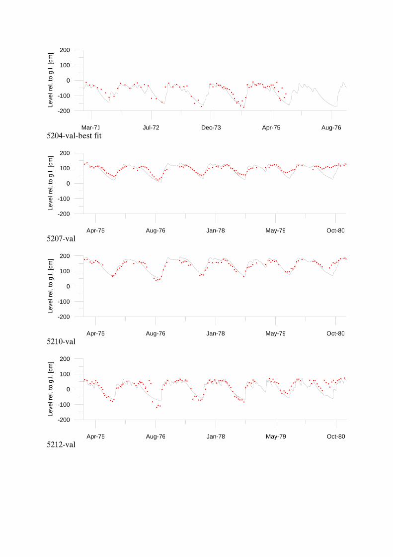
Mar-71 Jul-72 Dec-73 Apr-75 Aug-76

-200

-100

0

100

200Le

vel r

el. t

o g.

l. [c

m]

5204-val-best fit

Apr-75 Aug-76 Jan-78 May-79 Oct-80

-200

-100

0

100

200

Leve

l rel

. to

g.l.

[cm

]

5207-val

Apr-75 Aug-76 Jan-78 May-79 Oct-80

-200

-100

0

100

200

Leve

l rel

. to

g.l.

[cm

]

5210-val

Apr-75 Aug-76 Jan-78 May-79 Oct-80

-200

-100

0

100

200

Leve

l rel

. to

g.l.

[cm

]

5212-val

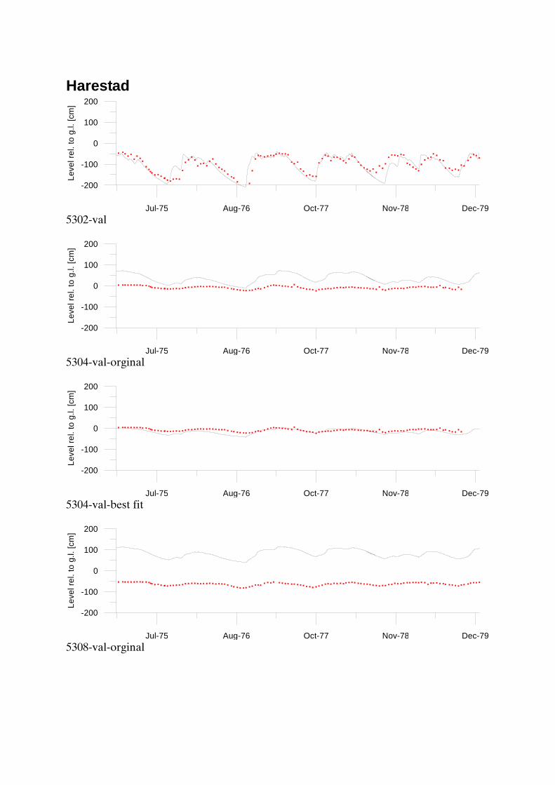
Harestad

Jul-75 Aug-76 Oct-77 Nov-78 Dec-79

-200

-100

0

100

200

Leve

l rel

. to

g.l.

[cm

]

5302-val

Jul-75 Aug-76 Oct-77 Nov-78 Dec-79

-200

-100

0

100

200

Leve

l rel

. to

g.l.

[cm

]

5304-val-orginal

Jul-75 Aug-76 Oct-77 Nov-78 Dec-79

-200

-100

0

100

200

Leve

l rel

. to

g.l.

[cm

]

5304-val-best fit

Jul-75 Aug-76 Oct-77 Nov-78 Dec-79

-200

-100

0

100

200

Leve

l rel

. to

g.l.

[cm

]

5308-val-orginal

Jul-75 Aug-76 Oct-77 Nov-78 Dec-79

-200

-100

0

100

200Le

vel r

el.

to g

.l. [c

m]

5304-val-one observation

Jul-75 Aug-76 Oct-77 Nov-78 Dec-79

-200

-100

0

100

200

Leve

l rel

. to

g.l.

[cm

]

5308-val-best fit

Jul-75 Aug-76 Oct-77 Nov-78 Dec-79

-200

-100

0

100

200

Leve

l rel

. to

g.l.

[cm

]

5309-val

Jul-75 Aug-76 Oct-77 Nov-78 Dec-79

-200

-100

0

100

200

Leve

l rel

. to

g.l.

[cm

]

5312-val-orginal

Jul-75 Aug-76 Oct-77 Nov-78 Dec-79

-200

-100

0

100

200Le

vel r

el. t

o g.

l. [c

m]

5312-val-best fit

Jul-75 Aug-76 Oct-77 Nov-78 Dec-79

-200

-100

0

100

200

Leve

l rel

. to

g.l.

[cm

]

5313-val

Statens geotekniska institutSwedish Geotechnical Institute

SE-581 93 Linköping, SwedenTel: 013-20 18 00, Int + 46 13 201800Fax: 013-20 19 14, Int + 46 13 201914

E-mail: sgi@swedgeo.se Internet: www.swedgeo.se