Estimation of environmental contours using a block

OMAE®39th International Conference on Ocean, Offshore & Arctic Engineering

Estimation of environmental

contours using a block

resampling method

OMAE2020-18308OMAE Virtual Conference: 3 – 7 August 2020

Ed MackayUniversity of Exeter, UK

Philip JonathanLancaster University, UKShell Research Ltd, UK


Overview

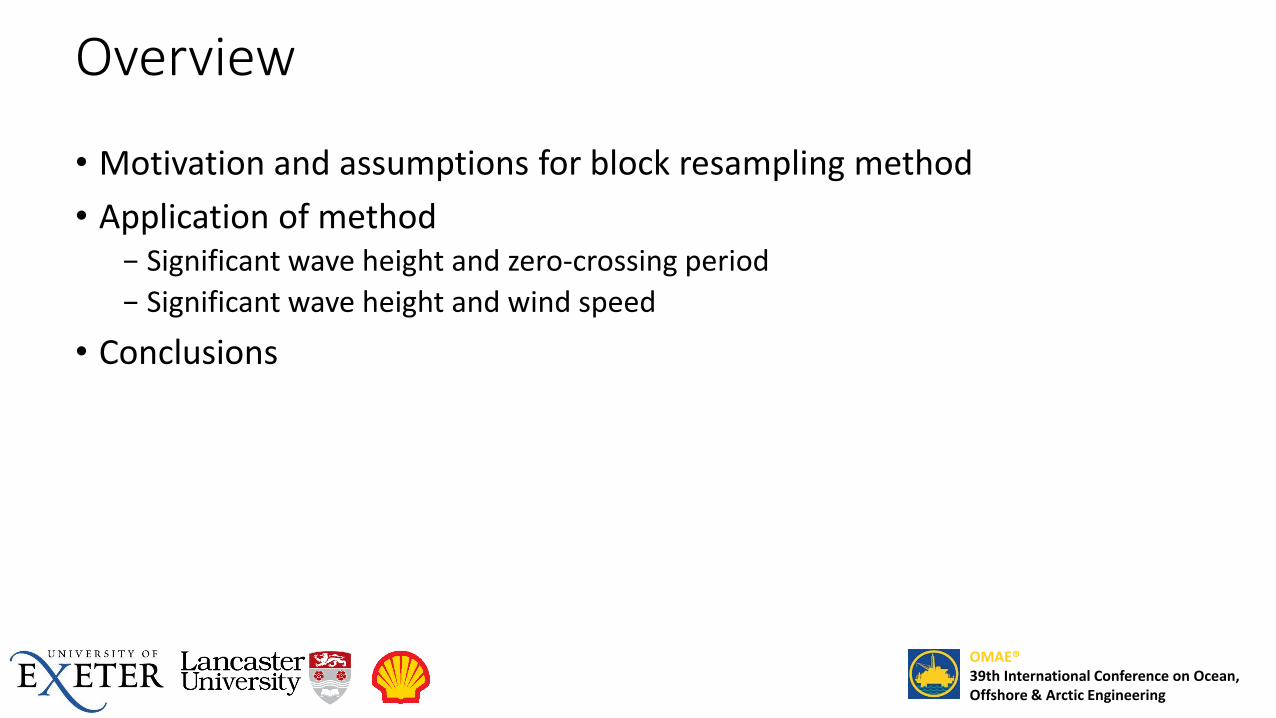
• Motivation and assumptions for block resampling method

• Application of method− Significant wave height and zero-crossing period

− Significant wave height and wind speed

• Conclusions


Motivation

• Common approach for deriving environmental contours is to fit a global model to all observations

• Several disadvantages to this approach− Fit to all observations doesn’t guarantee good fit to tail

▪ This is the region we are most interested in

Exce

ed

ance

pro

bab

ility


Motivation




− Does not account for serial correlation in data▪ Leads to positive bias in estimates of occurrence of extreme conditions


Motivation




− Does not account for serial correlation in data▪ Leads to positive bias in estimates of occurrence of extreme conditions

− Often require prior assumptions about dependence structure between variables▪ Many datasets exhibit complex dependence structures


1. Time series divided into non-overlapping blocks

2. Models fit to block-peak variables

3. Joint distribution of all data recovered by:a) Simulation of peak variables under fitted model

b) Resampling measured blocks with “similar” peak values

c) Rescaling measured blocks to match simulated peak values

Block resampling method

Advantages• Better justification for

asymptotic models• Creates time series

outputs for analysis of long term extreme response

• Short-term dependence structure resampled rather than modelled explicitly


Blocking method


Blocking method1. Identify peaks in one variable

▪ Defined as local maxima separated by min 5 days




2. Define dividing points of blocks as times of min Hs between adjacent peaks




2. Define dividing points of blocks as times of min Hs between adjacent peaks

3. Find peaks of other variables within each block▪ Peaks within blocks need not be

concurrent


3) Transform to standardLaplace margins

1) Find block-peak values2) Fit marginal models to peaks

4) Fit joint model5) Simulate from joint model6) Identify 𝑛 blocks with closest peaks

(Euclidean distance on Laplace margins)7) Select one of 𝑛 closest blocks at random8) Scale block so that peak values match

Resampling of measured blocks


• Blocks rescaled by ratio of simulated to measured peaks:

𝐻𝑠,𝑟𝑒𝑠𝑐𝑎𝑙𝑒𝑑 =𝐻𝑠,𝑠𝑖𝑚𝑝𝑒𝑎𝑘

𝐻𝑠,𝑚𝑒𝑎𝑠𝑝𝑒𝑎𝑘 𝐻𝑠,𝑚𝑒𝑎𝑠

𝑈10,𝑟𝑒𝑠𝑐𝑎𝑙𝑒𝑑 =𝑈10,𝑠𝑖𝑚𝑝𝑒𝑎𝑘

𝑈10,𝑚𝑒𝑎𝑠𝑝𝑒𝑎𝑘

𝑈10,𝑚𝑒𝑎𝑠

Rescaling of measured blocks


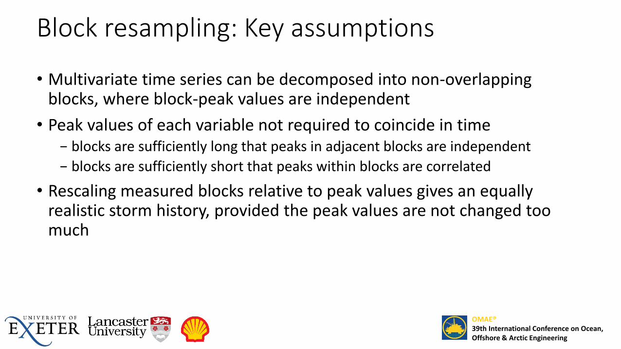
• Multivariate time series can be decomposed into non-overlapping blocks, where block-peak values are independent

• Peak values of each variable not required to coincide in time− blocks are sufficiently long that peaks in adjacent blocks are independent

− blocks are sufficiently short that peaks within blocks are correlated

• Rescaling measured blocks relative to peak values gives an equally realistic storm history, provided the peak values are not changed too much

Block resampling: Key assumptions


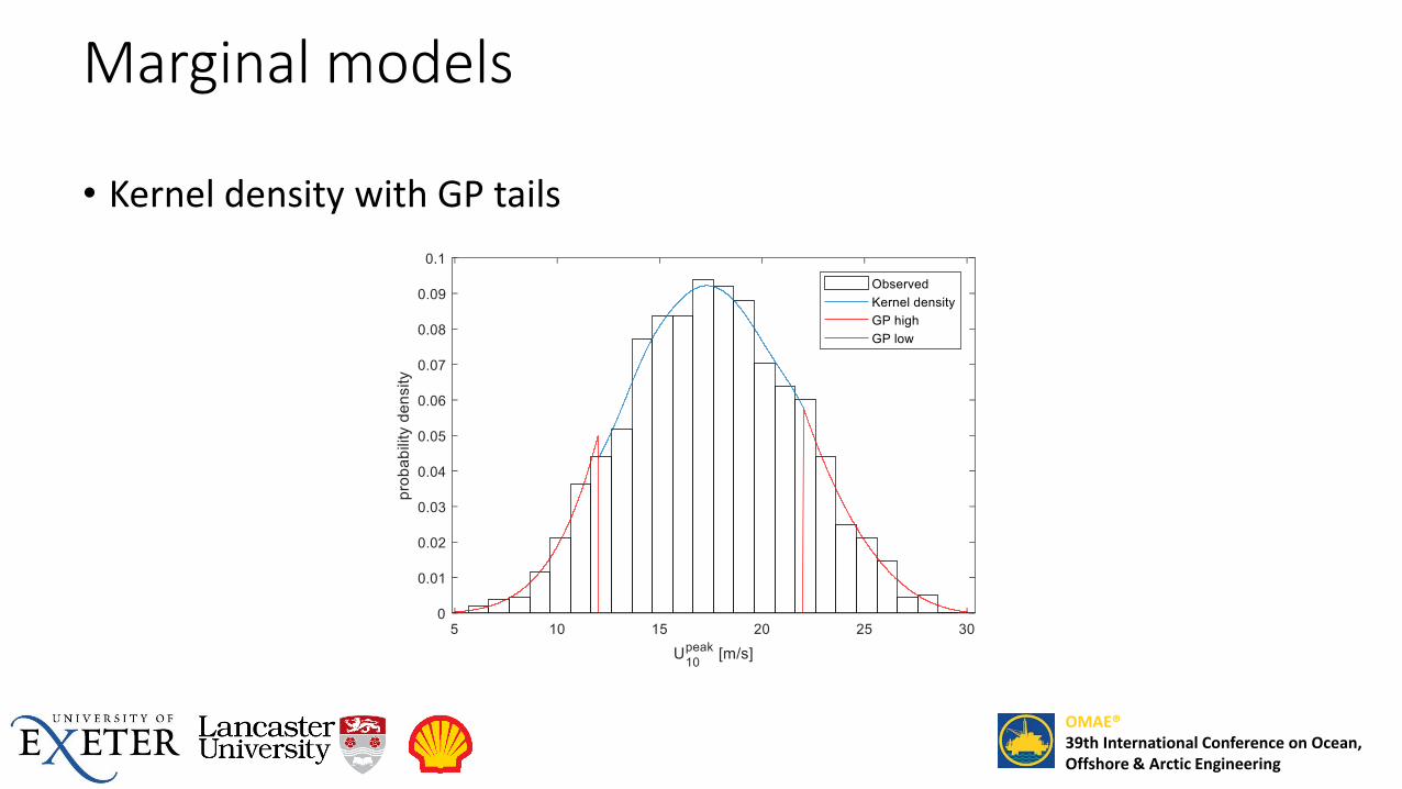
• Kernel density with GP tails

Marginal models


Joint models – example for Hs and Tz

𝑠 =2𝜋𝐻𝑠𝑔𝑇𝑧

2 𝑑2 = 𝐻𝑠2 +

1

2𝑇𝑧2

Frontiers of interest for extreme responses

Dataset A from [1]

[1] Haselsteiner et al. “A benchmarking exercise on estimating extreme environmental conditions”. OMAE2019–96523.


HT model 𝑝1 𝑥, 𝑦= 𝑝 𝑥 𝑝 𝑦 𝑥

𝑥

𝑦

Joint modelling approach

• Heffernan & Tawn (2004) model used to describe distribution of y conditional on extreme value of x



𝑥

𝑦

HT model 𝑝2 𝑥, 𝑦= 𝑝 𝑦 𝑝 𝑥 𝑦

Heffernan-Tawn model


• HT model also used for x given y



𝑥

𝑦


𝜃


Blended HT model



• HT models blended in overlapping region:

𝑝 𝑥, 𝑦 = 1 −2𝜃

𝜋𝑝1 𝑥, 𝑦 +

2𝜃

𝜋𝑝2 𝑥, 𝑦



𝑥

𝑦


𝜃


Blended HT model

Kernel density



• HT models blended in overlapping region:

𝑝 𝑥, 𝑦 = 1 −2𝜃

𝜋𝑝1 𝑥, 𝑦 +

2𝜃

𝜋𝑝2 𝑥, 𝑦

• Kernel density model used for non-extreme regions


• Blocks resampled from 10 closest blocks

• 1000 years of simulated data

• IFORM contours for 1, 5 and 50 years

• Note: IFORM not uniquely defined

− Rosenblatt transformation for 𝑇𝑧|𝐻𝑠 gives different contours to transformation of 𝐻𝑠|𝑇𝑧

− See [2] for details

Example contours

[2] Mackay & Haselsteiner, 2020. “Marginal and total exceedance probabilities for environmental contours”. Marine Structures (under review)


Example contours


Other results for contour benchmarking exercise


• Block resampling approach is capable of accurately reproducing both marginal and joint extremal characteristics of observed data

• Time series outputs – preserves ‘clustering’ properties of extremes

• Future work:− Resampling method without the need for pre-defining blocks

− Modelling of joint distribution without the need for multiple blended models

Conclusions


This work was funded under was funded under the UK Engineering and Physical Sciences Research Council (EPSRC) grant EP/R007519/1 and as part of the Tidal Stream Industry Energiser Project (TIGER), which has

received funding from the European Union’s INTERREG V A France (Channel) England Research and Innovation Programme, which is co-financed by the European Regional Development Fund (ERDF).

Acknowledgement

Documents

Estimation of environmental contours using a block