Estimation and Testing the Effect of Covariates in Accelerated Life Time Models under Censoring

Hannelore L i его

Mathematische Statistik und Wahrscheinlichkeitstheorie

UNIVERSITÄT P O T S D A M Institut für Mathematik

Universität Potsdam - Institut für Mathematik

Mathematische Statistik und Wahrscheinlichkeitstheorie

Estimation and Testing the Effect of Covariates in Accelerated Life Time Models under Censoring

Hannelore Liero

Institute of Mathematics, University of Potsdam

e-mail: liero@uni-potsdam.de

Preprint 2010/02

January 2010

Impressum

© Institut für Mathematik Potsdam, Januar 2010

Herausgeber: Mathematische Statistik und Wahrscheinlichkeitstheorie am Institut für Mathematik

Adresse:

Telefon: Fax: E-mail:

Universität Potsdam Am Neuen Palais 10 14469 Potsdam

+49-331-977 1500 +49-331-977 1578 neisse@math.uni-potsdam.de

ISSN 1613-3307

Estimation and Testing the Effect of Covariates in Accelerated Life Time Models under Censoring

Preliminary Version

Hannelore Liero Institute of Mathematics, University of Potsdam

e-mail: liero@uni-potsdam.de

Abstract The accelerated lifetime model is considered. To test the influence

of the covariate we transform the model in a regression model. Since censoring is allowed this approach leads to a goodness-of-fit problem for regression functions under censoring. So nonparametric estimation of regression functions under censoring is investigated, a limit theorem for a Z/2-distance is stated and a test procedure is formulated. Finally a Monte Carlo procedure is proposed.

Key words: Accelerated life time model; censoring; goodness-of-fit testing; nonparametric regression estimation; Monte Carlo testing AMS subject classification: Primary 62G10; Secondary 62N05

1 I n t r o d u c t i o n

We consider a life time model which describes the following situation: By some covariate X the time to failure may be accelerated or retarded relative to some baseline. The speeding up or slowing down is accomplished by some positive function ip, and we may write

T = T °

where To is the so-called baseline life time and T is the observable life time. We will assume that T is an absolute continuous random variable (r.v.) and that the covariate X does not depend on the time. For simplicity of presentation let X be one-dimensional.

1

For statistical application a suitable choice of the function tp is important and the problem of testing tp arises. A survey of test procedures for testing ip under different model assumptions is given in Liero H. and Liero M. (2008). The aim of the present paper is to propose a test procedures for testing whether the function rfi belongs to a pre-specified parametric class of functions

T = ty^(-) = / ? e R d } . (l)

For data without censoring this problem was already considered in Liero (2008). In this paper we assume that the independent and identically distributed life times Tj are subject to random right censoring, i.e. the observations are

Vi = min(Tj, d), Ai = l(Tj <Ct) and I j , i = 1 , . . . , n

where the C,'s are independent and identically distributed censoring times with distribution function G. Furthermore we assume that the T,'s and the Cj's are conditionally independent given the X,'s.

The inference is based on the log transformation of the lifetime model to a regression model: The conditional expectation of Y = logT given the covariate X has the form

E(Y\X = x) = fj. - logi(j(x) with ^ = - J logzdS0{z) = E(logT0),

where So is the survival function of the baseline life time To, and we can translate the considered problem into a problem of testing the regression function in a nonparametric regression model

Y = logT = m{X) + e,

where m(x) = /j, — log^(a;), and with e — log(To) — E(log(Tb))

£{e\X = x) = 0, and E(s2\X = x) = a2

for some a2 > 0. For identifiability we assume ^(0) = 1. Test problem (1) is translated into the following problem

H : m £ M. versus K : m$. M.

where

M = {m\m(-,(3,(j,) = -logV(s/3) + A», /? G Md,M e M},

2

that is we have to check whether the regression function has a parametric form or alternatively that this regression is nonparametric. As test statistic a weighted L2-distance between a parametric and the non-parametric regression estimator is proposed. To formulate the corresponding test procedure one has to investigate the properties of nonparametric esti­mators for regression functions under censoring. Therefore in Section 2 the nonparametric estimation of the regression function under censoring is considered. In Section 3 asymptotic properties of the nonparametric regres­sion estimator are presented; the main result is the asymptotic normality of the weighted ^-distance of the estimator. This limit theorem is based on a so-called asymptotic (conditional) i.i.d. representation of the difference between the estimator and the regression function. The test procedure is given in Section 4.

2 Nonparametric estimation of the regression function under censoring

We start with the a nonparametric estimator for the conditional distribution function of the transformed r.v. Y = log T. Such an estimator was intro­duced by Beran (1981). On one hand the Beran estimator can be regarded as an extension of the well-known Kaplan-Meier estimator proposed for models with censored data without covariates, on the other hand it is an extension of nonparametric estimators for conditional distributions functions studied for data sets without censoring. To define the Beran estimator it is useful to introduce the following functions and their estimators: The conditional distribution function of the r.v. Z = log V with V = min(T, C) is given by H(z\x) = P(Z < z\X = x) and estimated by the kernel estimator

Here K : K —> R is a kernel function, and bn is a sequence of bandwidths tending to zero as n —>• oo. The symbol " 1 " denotes the indicator function.

(2)

where Wbni are the kernel weights denned by

3

The estimator of the conditional subdistribution function Hu(z\x) — P(Z < z, A = 1\X = x) is given by

H%{z\x) = J2Wbni(^X1,...,Xn)l(Zi<z,Ai^l). (3)

For the conditional cumulative hazard function A we have for y < r

dF(s\x) fv dHu(s\x) . . . . p> dF{s\x) n> dl

H(s-\x)

where F denotes the conditional cdf of the transformed Y = l o g T and H(s^\x) = l im t | s H(t\x) , t x — iai{y\H{y\x) = 1} is the upper bound of the support of H(-\x). Replacing Hu and H by their estimators (2) and (3) leads to the weighted Nelson-Aalen type estimator for the conditional cumulative hazard function:

J-oo 1 - j H n ( s _ | a ; ) (4)

Now from the well-known relation between the cumulative hazard function and the survival function we obtain as estimator for Sy{y\x) = 1 — F(y\x) = P{Y > y\X = x)

SYn(y\x) = Yl(l- AAn(t|x)) (5) t<y

where AAn(t\x) — An(t\x) — An(t — \x) is the j u m p of A„(-|a;) at t. A n equivalent form of (5) is

Fn(y\x) = 1 - J] { Zi<V A,-=l

1 -Wbni(x,X)

ZHZj > Zi)wbnj(x,: 3

(6)

Note that for weights Wbni — ^ the estimator Fyn is the classical K a p l a n -Meier estimator; for Aj = 1 for all i the estimator Fn is the estimator of the conditional distribution function, and for Wj j = ^ and Aj = 1 for all i the estimator Fn is simply the empirical distribution function. Several authors considered the asymptotic behavior of Fn. Consistency of Fn(y\x) is proven for y < t x .

For simplicity we write X = (Xi,..,, X„).

4

The regression function m(x) = E(Y\X = x) is defined by JydF(y\x). However, for the estimation of m and the investigation of the properties of the resulting estimator the following identities are useful:

m(x) = E{Y\X = x)

ydF{y\x) (7)

and

= I F~l(u\x) Jo

m{x) = / F^iu^du (9)

where i 7 ' _ 1 (u|a;) — ini{y\F(y\x) > u}. To estimate m we replace F(y\x) in (7) by the Beran estimator and obtain as nonparametric estimator for m

= J ydFn(y\x). (10)

One can show that for this estimator the empirical versions of (8) and (9) hold, i.e.:

rhn{x) = W M ( x , X ) 1 ~ ZAi (11) rr{ 1 - Hn(Zi-\x)

and

mn(x) = f F^iu^du (12) Jo

where F~ x(tt|a;) = ini{y\Fn(y\x) > u}. W e see that as in the case without censoring the regression estimator is a weighted average; now, in the case with censoring an average of the uncensored observations. The weights depend on the kernel and on the ratio of the Kaplan- Meier estimator and the empirical df of the observations.

5

3 Properties of the nonparametric regression esti­mator

Gyorfi et al (2002) showed that an estimator of this type 2 is i n c o n s i s t e n t if the right endpoint of the support of F is smaller than that o f G. W e follow another approach than those authors. W e will use a conditional i.i.d. presentation of the difference between estimator and regression function; such a presentation is based on the corresponding result for the estimator Fn which is derived by Akritas and D u (2002). Since this presentation holds only for y < y*, where y* < svcpx TX we will truncate the estimator (due to the right censoring): Instead of m{x) = y dF(y\x) we estimate the function

m*(x ) = f ydF(y\x). (13) J—oo

The function m* is estimated by

(*) = rv*

J — CO ydFn(y\x) (14)

Before we state the results let us formulate the assumptions

A l The marginal density g of X is bounded on M. and twice continuously differentiable in a neighborhood of a set J and g{x) > c > 0 for some c and all i € l

A 2 The kernel i f is a symmetric density with compact support; further­more, it is twice continuously differentiable.

A 3 W e will need typical smoothness conditions on the functions H(-\-) and Hu (•{•). W e formulate here for a general (sub)distribution function L:

The derivatives

exist and are continuous for all y, and all x in a neighborhood of M..

Instead of kernel weights considered here they used nearest neighbor weights.

6

Lemma 3.1 Suppose that Al and A2 hold and that A3 is satisfied by H and Hu. then

n

m*n(x) - m*(x) = Yl Wbni(x,X) n^A^x) + Rn{x) (15) i=l

with

V(Zi, Ai\x) =y*(l - F(y*\x))Z(Zi, Auy*\x)

- fV {l-F(a\x))t{Zi,Ai,s\x)ds J—oo

where

l(Zi<s,Ai = l) _ fs l(Zj>w)dHu(w\x)

s v u ^ a w - { 1 _ H { Z i ] x ) ) y_oo ( 1 _ H H x ) ) 2 >

and where

supRn(x) = Op ((nbn)~% (log ) as n —» oo. x€l ^ '

Based on the presentation given in Lemma 3.1 we will prove the asymptotic normality of rhn(x) at an arbitrary fixed point x and a limit theorem for a weighted integrated squared error. Let us consider the conditional i.i.d. presentation as process and set

n

Mx) = ^Wb^XjviZuAilx). (16) i = l

In a first step we will split An in a stochastic and in a systematic part:

n

An{x) = ^TWbnifaX) M Z i . A i l x J - E M Z i . A i l a O l X i ] ) i = l n

+ ^2wbni(x,X)E[V(Zi,Ai\x)\Xi}. (17) *=i

Note that

Wbni(x,X) = 9n(x)

7

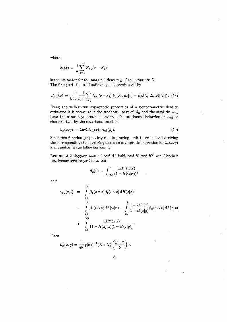
where

9n{x) = -Y^Kbn(X~Xj) 3=1

is the estimator for the marginal density g of the covariate X. The first part, the stochastic one, is approximated by

Am(x) = — L - i ^ K ^ i x - X i ) ( ^ ( Z i . A i l x J - E ^ Z i . A i l x J I X i ] ) . (18)

Using the well-known asymptotic properties of a nonparametric density estimator it is shown that the stochastic part of An and the statistic Ani have the same asymptotic behavior. The stochastic behavior of An\ is characterized by the covariance function

Since this function plays a key role in proving limit theorems and deriving the corresponding standardizing terms an asymptotic expression for Cn(x, y) is presented in the following lemma:

L e m m a 3.2 Suppose that Al and AS hold, and H and Hu are Lipschitz continuous with respect to x. Set

Cn(x,y) = Co\z(Ani(x),Ani{y)). (19)

and oo

—oo

s

—oo —oo

+ —oo

Then

8

y*2(l - F(y*\x))(l - F(y*\y))lxy{y\y*)

- y*(l-F(y*\x)) f (l-F(t\y))lxy(y*,t)dt

- y*(l-F(y*\y)) [ V (1-F(s\x))lxy(s,y*)ds (20) J—oo

+ F F (1-F(s\x))(l-F(t\y))lxy(s,t)dsdt) + o(n-1) J—ooJ —oo '

where K * K denotes the convolution.

The approximating statistic An\{x) is a sum of i.i.d. r.v. 's. Applying the central limit theorem we obtain immediately the asymptotic normality at a fixed point x:

^ W ^ N ( 0 , 1 ) . L,n(x, x)

After some transformations we obtain from Lemma 3.2 for x = y

Cn(x,x) =-b{g{x))-l(K *K)(0)

x £ y ( 1 _ W ) ) _ ^ ) . _ ^ +

=—K2p\x) + o{n-1). (21) no

with Ax(s; 1,*) = j f ( l - F(t\x)) dt and K2 = (K * K)(0). Hence

VnbAni(x) N(0,P2(X)K2). (22)

Since gn(x) is consistent,

Anl(x) = 0P{{nb)-1'2)

and

gn(x) - Egn(x) = 0P{{nb)-ll2)

9

we obtain n

(An(x) - ^ [ V w f o X j E ^ Z i , AOIJCi)) - Ani(x) i=l

= Aii(i) - i \ = Op{(nb) l).

Hence

/ n \

^& \ An(x) - ^W 6 i (a ; ,X ) E ( 7 7 x (Z i ,A i )|X i ) J N ( 0 , p 2 ( x ) « 2 ) . (23)

Now, to characterize the systematic part of the deviation define

B f , > fs dHu(t\x) fs H(t\x)dHu(t\x) / _ « , 1 - ff^x) . / _ « , ( l - # ( i | o : ) ) 2

and

dHu(t\x) , / * g ( t | g ) d g y ( t | g ) ( 1 - t f ( i | c c ) ) 2 '

„ , , fs dHu(t\x) fs

Using standard techniques for the investigation o f a bias we obtain the fol­lowing asymptotic expansion for the term YH=i Wbi{x,X)E(r]x(Zi, A , )|X j ) :

n

J^WwfoXJEMZi.AOIXi) = b2nB(x)Li2(K) + oP(b2

n), (24)

where

B(x) = ^ ^ ( l - F i y ^ B . i y ^ x ) - J " (l-F(s))B1(s,x)ds^ +

\ ^ ( 1 - F(y*))B2(y*, x) - j f J l - F ( s ) ) B 2 ( S , x ) d s j

and H2{K) = J u2K(u)du. If -> 0

n

V ^ ^ W ^ ^ ^ E ^ , ^ ) ^ ) = oP({nbl)ll2) = o P ( l ) , i=l

in other words, the systematic part is asymptotically negligible.

10

If nb^, —> c > 0 we have

and

nbAn(x) -^N(^B(X)(I2(K),P2{X)K2 (25)

B y Lemma 3.1 we conclude from the asymptotic behavior of An(x) to that of — m*(x) and formulate the following theorem:

Theorem 1 (Asymptotic normality at a fixed point) Under the as­sumptions given above and bn —> 0 and nbn —> o o

(i) Ifnbn -> 0 then

/nbn (K(x) ~ m*(x)) N ( 0 , K2 p\x)) with

p\x) = (g(x))-1 £jy*(l-F(y*\x))-Ax(S;y*))2^

(26)

dHu{s\x) -H(s\x))2'

(ii) / / nb^ —> c > 0 then

nbn « ( z ) - m*(x ) ) N ( v/ 5 J B ( x ) / x 2 ( i ; ! : ) , / 5 2 ( a ; ) K 2 ) . (27)

Remark: Consider the case without censoring. Using integration by parts we obtain for y* = o o , H = Hu = F

Thus, in this case Theorem 1 coincides with the well-known limit theorem stating asymptotic normality of nonparametric kernel regression estimators.

The asymptotic normality at a fixed point characterizes the local behavior. For testing the formulated hypothesis it seems to b e better to use a global

11

deviation measure. So, let us consider the integrated squared difference, weighted by a known function a with a(x) = 0 for x I:

Qn = J(K(x) ~ m*(x))2a(x)dx.

Heuristically speaking this is an infinite sum of squares of asymptotically normally distributed r.v. 's. which are asymptotically independent as bn

tends to zero. Thus Q n , properly standardized, converges in distribution to the standard normal distribution. Using the method proposed by Hall (1981) for proving the asymptotic normality of the integrated squared error of kernel density estimators one can show the following limit theorem

Theorem 2 (Asymptotic normality of the ISE) Under the assump-

Hons formulated above and nbn —> oo and n$bn —> 0

Qn = JK(^) - m*(x))2a(x)dx

n&y2(Q„ - e n ) ^ N ( 0 , ^ 2 )

= en{g,H,Hu;K,a,bn) = ( n 6 „ ) _ 1 K 2 Jp2(x)a(x)dx

with

v2

v2(g,H,Hu-K,a) = 2 k x Jp4(x) a2(x) àx

with KI = J(K * K)2(x) Ax.

4 Formulation of the test procedure

Let us apply the limit theorem for the I /2 -type distance of the truncated es­timator from the truncated regression function to formulate a test procedure for testing the hypothesis m £ A4. The alternative is characterized by the nonparametric estimator m*. Sup­pose the null hypothesis is true. The hypothetical function m*(-;,î9) is unknown. Firstly, one has to estimate the unknown parameter There

12

are several proposals in the literature to do this; we refer to Tsiatis (1990), Ritov (1990) or Bagdonavicius/Nikulin (2001). T h e basic idea is to replace the unknown cumulative hazard function by an efficient estimator depend­ing on $ and to estimate this unknown parameter then by the maximum likelihood method. The authors show that under suitable assumptions the resulting estimator is i /n-consistent, i.e.

y/n (FN ~ -&) = Op(1) as n ^ oo. (28)

The next step is to determine m* (•;$)• Wi th the estimator B the Breslow estimator for the cumulative hazard function of the unobservable r.v. To is constructed as follows:

ANO(T-J) = f -JO 1

dff&( 8 ; /3 )

-H„o(8-J) where

1 n

HN0(T-J) = - J2l(V0I<T) I=L

is the empirical distribution function of the estimated hypothetical baseline observations Vqj = VIIP(XI, 0), and

n ¿=1

is the corresponding estimator of the subdistribution of the uncensored observations. Then the baseline survival function is estimated by

Sofop) = - A A 0 ( s ; / 3 ) )

s<t and the hypothetical truncated regression function by

m * M ) = - fV ydSo(4>il>(x-J)) J—oo

•I o ip(x;3)

13

W e see, for y* —» oo the function m*(x;i9) converges to oo

logzd§o{z) — log ip(x; ¡3) = ¡1 — log tp (x; ¡3) = m{x\'d).

The test procedure has the following form: The hypothesis m £ M, that is I/J & T is rejected if the estimated Z/2-distance

Qn = Ji-K{x) - m*{x;$))2a(x)dx satisfies the inequality

where is the (1 — a)-quantile of the limiting distribution and en = en{9n,Hn,Hu,K,a,bn) and v2 = v2(gn,Hn,Hu ,K,a) are the estimated standardizing terms.

4.1 A proposal for a Monte Carlo procedure

Finally a Monte Carlo method for determining empirical p-values of the test procedure is proposed. The aim of this method is to generate data

(V*,X*r,A*ir), r = l,...,R, i = l,...,n

according to the hypothetical model . Based on these data the test statistics Q n i i • • • > Q n r > • • • i QnR 8 X 6 computed and from their empirical distribution the p-value is determined. The data can be constructed as follows:

1. Let (5 the estimator for (3 based on the original data. Construct the Breslow estimator Ao(-; ¡3) for the cumulative baseline hazard function. Then

S0(T-J) = - AA0(S-J)).

8<t 2. Generate data T$IR from the estimated survival function SO(T;/3) and

set

rp* _ Oir

14

3. Estimate the distribution function of the Cj by the weighted Kaplan-Meier estimator Gn and generate censoring variables C*r from the estimated survival function Gn.

4. Finally set

V*r = min(T i *, C*r), A*r = l(T*r < C*r), X*r = Xi.

As of yet this M C procedure is only a proposal and further investigations should be pursued.

References

[1] M. G. Akritas and Y . Du. IID representation of the conditional Kaplan-Meier process for arbitrary distributions. Mathematical Methods in Statistics, 11:152-182, 2002.

[2] V . Bagdonavicius and M. Nikulin. Accelerated Life Models. Springer Series in Statistics. Chapman and Hall, 2001.

[3] R. Beran. Nonparametric regression with randomly censored survival data. Technical report, Univ. California, Berkeley, 1981.

[4] L. Gyorfi, M . Kohler, A. Krzyzak, and H. Walk. A Distribution-Free Theory of Nonparametric Regression. Springer Series in Statistics. Springer, 2002.

[5] P. Hall. Central limit theorem for integrated square error of multivariate nonparametric density estimators. J. Multivariate Analysis, 14:1-16, 1984.

[6] H. Liero. Testing in nonparametric accelerated life time models. Austrian Journal of Statistics, 37(1), 2008.

[7] H. Liero and M . Liero. Testing the influence function in accelerated life time models. In F. Vonta, M. Nikulin, N. Limnios, and C. Huber, editors, Statistical models and methods for biomedical and technical systems. Birkhauser, 2008.

15

[8] Y . Ritov. Estimation in a linear regression model with censored data. Ann. Statist, 18:303-328, 1990.

[9] A . A . Tsiatis. Estimating regression parameters using linear rank tests for censored data. Ann. Statist, 18:354-372, 1990.

16