1

Estimating Total System Damping for Soil-Structure Interaction Systems

Farhang Ostadan,a) Nan Deng,b) and Jose M. Roessetc)

For a realistic soil-structure interaction (SSI) analysis, material damping in the

soils and structural materials as well as the foundation radiation damping should

be considered. Estimating total system damping is often difficult due to complex

interplay of material damping and radiation damping in the dynamic solution. In

practice, however, an estimate of total system damping is frequently needed for

evaluation of SSI effects and for detailed linear or nonlinear structural analysis in

order to develop realistic results. The simple methods typically used to estimate

structural damping from the dynamic response of the structure often fail to yield

realistic system damping mainly due to frequency dependency of the foundation

stiffness and dashpot parameters. In this paper a summary of series of parametric

studies is discussed and an effective approach to estimate system damping for SSI

systems is presented. The accuracy of the method is verified using a model of a

large concrete structure on a layered soil site.

INTRODUCTION

Regulations for the seismic design of Nuclear Power Plants permit soil-structure

interaction (SSI) analyses in the frequency domain, with the full effects of radiation damping,

without any limitations. The frequency domain solutions are generally more suitable for

incorporation the damping effects since these solutions incorporate the frequency dependency

of the foundation stiffness and damping rigorously and can handle the far field boundary

conditions more accurately. There are numerous publications reporting the foundation

stiffness and damping for surface or embedded foundation on uniform halfspace or layered

sites using the frequency domain approach.

a) Bechtel, 50 Beale St., San Francisco, CA 94119 b) Bechtel, 50 Beale St., San Francisco, CA 94119 c)Texas A&M University, College Station, Texas 77843

Proceedings Third UJNR Workshop on Soil-Structure Interaction, March 29-30, 2004, Menlo Park, California, USA.

2

On the other hand analyses in the time domain, and particularly modal analysis that

requires specification of damping for each mode, had limits of 15 % or even 10 % imposed

on the damping. Because radiation damping could be significant in some cases, leading at

times to effective values of damping in the first mode of 20 % or 25 % under horizontal

excitation and up to 50 % or more in vertical vibration, the results of both types of analyses

could be very different, with the time domain solution overly conservative. There was little

interest or incentive in finding what the effective values of damping implicit in the frequency

domain approach were or what should be the values of modal damping to be used in the time

domain models to yield similar results. Analyses in time and frequency domain cannot

produce identical results because each one involves different approximations. One can

obtain, however, very similar and reasonable results if consistent assumptions are made and

the values of the different model parameters (frequency independent foundation stiffness,

damping, etc.) are wisely selected. To do this it is necessary to look in more detail at the

effective damping implicit in frequency domain SSI analyses.

Currently dynamic non-destructive testing is increasingly used to assess the condition of

existing structures for health monitoring and damage assessment. The structure may be

excited by very small amplitude dynamic loads, by ambient vibrations or by actual

earthquakes. Its characteristics are to be determined from the recorded motions at various

points where sensors are installed. These characteristics are often expressed in terms of the

natural frequencies, mode shapes and modal damping values, which may vary in time

depending on the level of excitation. The experimental determination of damping values for

multi-degree of freedom systems without a unique, clearly defined, source of energy

dissipation represents a problem similar to that encountered when attempting to specify

modal damping for SSI analyses in the time domain.

The objectives of this work are to explore the effective values of system damping implicit

in SSI systems in the frequency domain, to compare the results of different procedures to

estimate damping from response records, and to compare the results of SSI analyses in the

frequency domain with those of time domain solutions using realistic parameters. The

emphasis is placed on estimating the total system damping for the key dynamic structural

responses that inherently include the effects of material damping in the system, the radiation

damping due to the SSI effects recognizing complex contribution of the SSI modes and the

structural deformation modes in the response. In this paper first the types of damping and

3

modeling of damping for dynamic analysis are discussed. Next the simple methods typically

used to estimate damping from structural responses are discussed. A series of parametric

studies are performed and the results are discussed to evaluate the merit of each method to

estimate total system damping. From the parametric study, the most effective method is

identified. The accuracy of the method is tested by applying it to a lumped parameter SSI

model to estimate system damping using the time integration method and comparing a key

response to the complete SSI solution of the problem. Unless otherwise noted, all computer

analyses in this paper are using SASSI2000 (Lysmer et. al, 1999) computer program.

DAMPING AS A MEASURE OF ENEGY DISSIPATION

Treatment of damping as a means to model energy dissipation starts in structural

dynamics texts by considering a single degree of freedom system with a viscous dashpot. The

dashpot has a constant 'c' and a resisting force directly proportional to the rate of deformation

(the relative velocity of the mass with respect to the base). This is often referred to as linear

viscous damping. One can define a fraction of critical damping β as

kc

mc

kmc

2220

0

ωω

β === (1)

where k is the stiffness of the system, m the mass and ω0 the undamped natural frequency of

the system. When dealing with this damping the physical constant is the dashpot value 'c'.

The value of β is not only a property of the dashpot but also depends on the rest of the

system. It can be easily seen that for a fixed c, defining a dashpot, if both k and m vary

proportionally, maintaining the natural frequency constant, the fraction of critical damping

will decrease with increasing k and m; if m is maintained constant and k is varied, changing

the natural frequency, the value of β will decrease with increasing natural frequency (mass

proportional damping); if k is kept constant and m varies, changing again the natural

frequency, β will increase with frequency (stiffness proportional damping).

It should be noticed that in reality viscous forces (such as drag forces induced by motions

in a fluid) are often proportional to the velocity raised to a certain power and are therefore

nonlinear. More importantly unless one attaches actual viscous dampers at different points of

the structure, most of the energy dissipation in structures does not occur in the form of linear

viscous damping. This model is used primarily because it leads to a linear differential

equation that can be easily solved analytically. It is, however, commonly accepted and most

4

engineers tend to think of damping in terms of the fraction of critical damping. Alternative

forms are frictional (Coulomb) damping, hysteretic damping associated with nonlinear

behavior and hysteresis loops in the force displacement relation of the stiffness, and radiation

damping due to radiation of waves in a continuous medium away from the area of the

excitation. A mathematical idealization, without a clear physical model, is the linear

hysteretic damping D (sometimes referred to as structural or material damping). It tries to

simulate the behavior of a hysteretic nonlinear system under steady state vibrations with

fixed amplitude (the value of the damping would be a function of the amplitude). The linear

hysteretic damping is defined as

D= Ed/ (4πEs) (2) where Ed is the energy dissipated per cycle (area of the hysteresis loop) and Es is the

maximum strain energy (assuming an equivalent linear system with the secant stiffness and

the same amplitude of vibration). This damping is then included in dynamic analyses (or

wave propagation studies) in the frequency domain using complex moduli of the form

E(1+2iD) or G(1+2iD) where E and G are the Young’s and shear modulus of the material.

This is what is commonly done to model the soil in soil amplification or soil structure

interaction analyses with most of the available software in the public domain. The damping

D is independent of frequency. Considering instead the cyclic behavior of a system with

linear viscous damping and the same amplitude of vibration, and applying the above formula

one would find that in that case

D=β ω /ω0 (3)

where ω is the frequency of the steady state vibration and ω0 is the natural frequency of the

single degree of freedom viscous system. This implies that to simulate the effect of viscous

damping with a linear hysteretic model D would have to increase proportionally with

frequency and to simulate hysteretic (frequency independent) damping with a linear viscous

system β would have to decrease with increasing frequency. Linear hysteretic damping is

only properly defined in the frequency domain and under steady state vibrations although it is

used for transient dynamic analyses with the Fourier transform. Since damping is

particularly important at or near resonance it is common to make simply D=β. This would

result in two systems with the same amplitude of response at resonance but different behavior

at other frequencies.

5

In SSI problems energy is dissipated in the structure through friction and nonlinear

behavior and in the soil through nonlinear behavior and radiation. To arrive at an effective

value of damping for the complete system it is necessary to combine these different

contributions. The internal damping in the structure is often assumed to be viscous although

a hysteretic model would be more realistic. With viscous damping its contribution to the

damping of the complete system is multiplied by the ratio of the combined natural frequency

to that of the structure by itself on a rigid base raised to the cube. For the hysteretic case the

factor would be only squared. The internal soil damping is normally considered using linear

hysteretic damping (complex moduli) with analyses in the frequency domain. For time

domain analyses it is common to use Rayleigh damping attempting to maintain it nearly

constant and close to the desired value over the range of frequencies of interest. When a

steady state harmonic load P is applied on top of a rigid mat the resulting displacement will

reach after a short while a steady state condition. In this range the displacement will have an

amplitude U and will be out of phase with the applied force by an angle φ (or a time lag τ =

φ/ω if ω is the frequency of vibration). It is common to express the foundation stiffness in

the form

k= kreal+ i kimag = P/U cosφ + i P/U sinφ (4)

where the ratio P/U and the angle φ are in general functions of the frequency. By analogy the

dynamic stiffness of a single degree of freedom system with linear viscous damping would be

kdyn= k - m ω2 + i ω c (5)

and for a system with hysteretic damping

kdyn= k - m ω2 + 2i D k (6)

It should be noticed that for the system with linear viscous damping the imaginary part of

the dynamic stiffness increases proportionally with the frequency of vibration. The plot of

imaginary stiffness versus frequency would be a sloping straight line. Dividing it by ω one

obtains a horizontal line (independent of frequency) with the value of the dashpot constant c.

For the linear hysteretic system on the other hand the imaginary part is constant and dividing

it by the frequency one gets a hyperbola with very large values for low frequencies and

tending to 0 as the frequency increases. A system with both viscous and hysteretic damping

would have an imaginary stiffness consisting of the sum of a constant and a sloping line with

slope c. Dividing it by ω would yield a hyperbola tending to a constant value c.

6

When applying horizontal harmonic forces to a rigid mat foundation on the surface of an

elastic half space the real part of the stiffness is essentially constant (it actually has a small

variation with frequency) and the imaginary part is essentially a straight line. This implies

that the foundation can be modeled as a spring and a viscous dashpot. If the soil had some

internal damping, of a hysteretic nature, the imaginary part of the stiffness would be again the

sum of a constant and a term linearly proportional to ω and dividing it by ω would result in a

hyperbola. The limiting value of the hyperbola as the frequency increases represents the

radiation damping. When applying on the other hand a vertical force to the foundation if the

soil has a Poisson’s ratio of the order of 0.4 or higher the real part of the stiffness looks like a

second degree parabola with negative curvature suggesting a model with a spring and a mass

(added mass of soil). In this case the dynamic stiffness can become negative for high

frequencies much as the value of k-mω2 would become negative for a single degree of

freedom system. In attempting to define the effective damping for a rigid block placed on top

of the foundation one should add the mass of soil to that of the block and consider the static

stiffness instead of using a zero or negative stiffness. For a foundation on the surface of a

soil layer of finite depth (resting on much stiffer, nearly rigid rock) the real and imaginary

parts of the stiffness will exhibit fluctuations associated with the natural frequencies of the

layer. For a soil without any internal damping the stiffness would become 0 at the soil

natural frequency. Below a threshold frequency (the fundamental frequency of the soil layer

in shear for the horizontal case, the corresponding frequency in compression-dilatation for

the vertical and rocking cases if Poisson’s ratio is 0.3 or less, and an intermediate frequency

for higher Poisson’s ratios) there will be no radiation and the damping will be associated only

with the internal, hysteretic, dissipation of energy in the soil. Above the threshold frequency

there will be radiation and the results will be similar to those of the half space except for their

fluctuations. The interpretation of what is the effective damping is more difficult for these

cases.

MEASUREMENT OF DAMPING

Measurement of damping is carried out either through free vibration or forced vibration

steady state tests. Under free vibrations a system with linear viscous damping experiences an

exponential decay in amplitude. The natural logarithm of the ratio of the amplitude of a peak

to that of the next one of the same sign would be then 2πβ/(1-β2)0.5 or approximately 2πβ for

low values of damping. The logarithm of the ratio of the amplitude of one positive peak to

7

that of the next negative one (or valley) would be half. The logarithm of the ratio of the

amplitude of a peak to that of the peak n cycles later would be n times this quantity. If the

damping is not of a linear viscous nature the ratio of the amplitudes of two consecutive peaks

would not be constant. In laboratory free decay tests it is common to observe a variation in

this ratio and to take an average over various cycles. Because these free vibrations take place

at the natural frequency of the sample one could assume that the measured β can also be D.

In laboratory steady state cyclic tests at a given frequency one can obtain the force

deformation diagrams for each cycle and compute the energy dissipated (area of the

hysteresis loop) and the equivalent secant stiffness (to compute the maximum strain energy).

The damping ratio D can then be directly calculated. This is what is normally done to

determine for different soils the variation of the effective shear modulus and damping with

the level of shear strains (and frequency in some cases). An alternative is to determine

experimentally the response of the sample to harmonic excitation with different frequencies,

plotting the displacement amplitude (divided by the amplitude of the applied force) versus

frequency. This is the traditional amplification function for the response of a single degree of

freedom system to a harmonic steady state excitation. The peak in the response occurs at a

frequency ω0 (1-2β2)0.5 or approximately ω0 (undamped natural frequency) for low values of

damping. Its value is 1/2β(1-β2)0.5. The value of the amplification at the frequency ω0 would

be exactly 1/2β. It is common as a result to measure the amplitude of the peak U and to

calculate the damping as 1/2U. Because the exact peak may be difficult to obtain an

alternative is to use the half power bandwidth method (Clough and Penzien, 1993, Chopra,

1995). In this case calling ω2 and ω1 the frequencies at which the amplitude would be 2

1 U

the damping can be obtained approximately (again for low values of damping) as β= (ω2-

ω1)/(ω2+ ω1). These expressions assume again linear viscous damping and a single degree of

freedom system. When dealing with experimental frequency response curves obtained in the

field (either applying very small amplitude harmonic excitations, from records of ambient

vibrations, or from records of response to actual earthquakes) it is common to use this

approach to determine the effective damping in each mode. It is common to assume that the

first peak is only affected by the first mode, the second by the first 2 modes, and so on. The

fact that it is no longer a single degree of freedom system and that the damping is not

primarily of a viscous nature make the reliability of the estimates somewhat questionable.

8

In SSI problems if a rigid mass M resting on a mat foundation on the surface of an elastic

halfspace is subjected to horizontal excitation, calling kreal and kimag the real and imaginary

part of the foundation stiffness and c=kimag/ω based on the previous considerations, the

fraction of critical damping for the system

kMc

2=β (7)

would be approximately constant if M is constant. On the other hand if M changed so as to

change the natural frequency of the system with k=Mω02, β would increase linearly with the

natural frequency and become

β = cω0 /2k (8)

If the soil had some internal damping of a hysteretic nature β so defined would look like a

hyperbola as a function of frequency with very large values at low frequencies. It would be

more logical then to separate first the hysteretic component (corresponding to the value of

kimag at low frequencies divided by 2 k, then apply the above equation to the remaining c and

add both results. When dealing with vertical vibration and a soil with Poisson's ration of 0.4

or more one should use the static value of the real stiffness and add to the rigid mass M the

added mass of soil in order to estimate the damping (rather than dividing by a k that could

become 0 or negative).

When dealing with a soil layer of finite depth the interpretation of the damping becomes

more difficult because of the fluctuations in the real and imaginary parts of the stiffness with

frequency. One could use the value of the variable k at each frequency or consider instead

the static value and consider the difference between the static and the dynamic values an

added mass of soil multiplied by the square of the frequency, adding it to the value of the

rigid mass.

It is noted that other simple relationships have been developed to estimate system

damping for SSI systems on the frequency by frequency basis involving structures with

single degree of freedom such as those developed by Roesset (NUREG/CR 1780, 1980).

However, the purpose of this paper is to develop a simple method to estimate the total system

damping as it relates to the final dynamic structural responses (such as the acceleration

response spectra at selected mass points). Such responses obviously include the effects of

material damping in the soil and structure, radiation damping of the foundation and the

9

combined modal effects of structural deformation as well as rigid body SSI motion. As

shown in this paper, a more reliable way to estimate the system damping would be to subject

the system to an impact load and study its free vibration and assess the damping from decay

of the free vibration response.

PARAMETRIC STUDY

A total of five simple systems shown in Figure 1 have been analyzed. The systems

considered are as follows. A single degree-of-freedom (SDOF) system consisting of a

lumped mass and a spring as depicted by Case 1 in Figure 1 was analyzed. The base of the

model is fixed and has a fixed base natural frequency of 4 Hz. The material damping used is

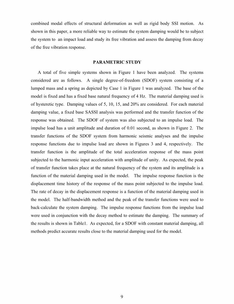
of hysteretic type. Damping values of 5, 10, 15, and 20% are considered. For each material

damping value, a fixed base SASSI analysis was performed and the transfer function of the

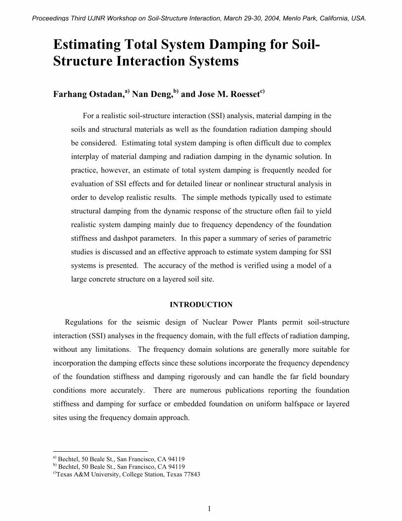
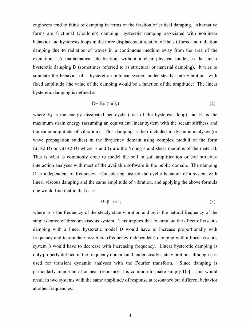
response was obtained. The SDOF of system was also subjected to an impulse load. The

impulse load has a unit amplitude and duration of 0.01 second, as shown in Figure 2. The

transfer functions of the SDOF system from harmonic seismic analyses and the impulse

response functions due to impulse load are shown in Figures 3 and 4, respectively. The

transfer function is the amplitude of the total acceleration response of the mass point

subjected to the harmonic input acceleration with amplitude of unity. As expected, the peak

of transfer function takes place at the natural frequency of the system and its amplitude is a

function of the material damping used in the model. The impulse response function is the

displacement time history of the response of the mass point subjected to the impulse load.

The rate of decay in the displacement response is a function of the material damping used in

the model. The half-bandwidth method and the peak of the transfer functions were used to

back-calculate the system damping. The impulse response functions from the impulse load

were used in conjunction with the decay method to estimate the damping. The summary of

the results is shown in Table1. As expected, for a SDOF with constant material damping, all

methods predict accurate results close to the material damping used for the model.

10

Figure 1. Numerical Models Considered for Parametric Study

Rigid Base

M

K, β

F(t), d(t)

Case 1

Case 2 Case 3

Case 4 Case 5

R = 30 ft.

Homogeneous Halfspace

Vs = 2000 ft/s

ν = 1/3

β = 0.05

γ = 120 pcf

Rigid Massless Foundation

R = 30 ft.

Homogeneous Layer

Vs = 2000 ft/s

ν = 1/3

β = 0.05

γ = 120 pcf

Rigid Massless Foundation

H = 90 ft.

R = 30 ft.

Homogeneous HalfspaceVs = 2000 ft/sν = 1/3β = 0.05γ = 120 pcf

Rigid Massless Foundation

D = 30 ft.

R = 30 ft.

Homogeneous LayerVs = 2000 ft/sν = 1/3β = 0.05γ = 120 pcf

Rigid Massless Foundation

H = 90 ft.

D = 30 ft.

11

Figure 2. Impulse load to compute impulse response function

Figure 3. Transfer function results for fixed base SDOF system

0

0.2

0.4

0.6

0.8

1

1.2

0 0.2 0.4 0.6 0.8 1 1.2 1.4 1.6 1.8 2

Time (second)

Nor

mal

ized

Am

plitu

de

0

2

4

6

8

10

12

0 1 2 3 4 5 6 7 8 9 10

Frequency (Hz)

Tran

sfer

Fun

ctio

n A

mpl

itude

5% Damping

10% Damping

15% Damping

20% Damping

12

Figure 4. Impulse response for SDOF fixed base system

Table 1. Damping computed for fixed base SDOF system using 3 methods

Next a surface rigid circular foundation was analyzed. In Case 2 (see Figure 1), the

foundation is located on the surface of a uniform elastic halfspace with hysteretic material

damping of 5%. In Case 3, the same foundation is placed on the surface of a layered soil

resting on rigid base. The thickness of the soil layer is three times the radius of the

foundation. Equations 4, 5 and 6 with m = 0 are used to obtain the stiffness (kreal) and

dashpot coefficients, c. The material damping for soils is included in the SASSI soil

properties using the complex soil moduli. In SASSI analysis, a unit amplitude horizontal

-1.5

-1.0

-0.5

0.0

0.5

1.0

1.5

0.50 0.75 1.00 1.25 1.50 1.75 2.00

Time (second)

Impu

lse

Res

pons

e, U

5% Damping

10% Damping

15% Damping

20% Damping

Decay Fit

β = 5.0%

Approach 5.0 10.0 15.0 20.0

Half Band 4.8% 9.7% 15.9% 22.3%

1/(2*Umax) 5.0% 9.9% 14.7% 19.5%

Decay of Motion 5.0% 10.0% 14.9% 19.6%

Given Structural Damping(%)

13

harmonic load is applied to the foundation and from the real and imaginary parts of the

displacement results k and c are computed for each frequency. The results are shown in

Figures 5 and 6. For Case 3 the stiffness and dashpot coefficients show a much larger

frequency dependency than in Case 2, the uniform halfspace case. Following the impedance

analysis, each foundation model was modified by adding a single mass point at the center. A

total of 5 mass values were used in separate analyses. The mass values were chosen to have

the foundation undamped natural frequencies of 2, 4, 6, 8, and 10 Hz to cover a wide range of

natural frequencies. Each foundation system with the mass point described above was

analyzed under harmonic seismic loading and was also subjected to the impulse loading

shown in Figure 2. The results of analyses in terms of absolute acceleration transfer

functions for Cases 2 and 3 are shown in Figures 7 and 8, respectively.

14

Figure 5. Horizontal foundation stiffness for Cases 2 and 3

Figure 6. Horizontal foundation dashpot coefficient for Cases 2 and 3

0.0E+00

5.0E+08

1.0E+09

1.5E+09

2.0E+09

2.5E+09

3.0E+09

0 2 4 6 8 10 12 14 16 18 20

Frequency (Hz)

Stiff

ness

(kip

s./ft

.)

Kx - Surface Fdn on Halfspace

Kx - Surface Fdn on H/R=3 Layer

0.0E+00

1.0E+07

2.0E+07

3.0E+07

4.0E+07

5.0E+07

6.0E+07

0 2 4 6 8 10 12 14 16 18 20

Frequency (Hz)

Das

hpot

C (k

ips-

sec.

/ft.)

Cx - Surface Fdn on Halfspace

Cx - Surface Fdn on H/R=3 Layer

15

Figure 7. Transfer function amplitude for Case 2 (surface foundation on halfpace)

Figure 8. Transfer function amplitude for Case 3 (surface foundation on H/R=3)

The results show the effect of changing the mass points from one value to another. The

results in terms of impulse response function are shown in Figures 9 and 10, respectively.

0

1

2

3

4

5

6

0 2 4 6 8 10 12 14 16 18 20

Frequency (Hz)

Tran

sfer

Fun

ctio

n A

mpl

itude

With 2Hz Mass

With 4Hz Mass

With 6Hz Mass

With 8Hz Mass

With 10Hz Mass

0

2

4

6

8

10

12

0 2 4 6 8 10 12 14 16 18 20

Frequency (Hz)

Tran

sfer

Fun

ctio

n A

mpl

itude

With 2Hz Mass

With 4Hz Mass

With 6Hz Mass

With 8Hz Mass

With 10Hz Mass

16

Figure 9. Impulse response functions for Case 2 (surface foundation on halfpace)

Figure 10. Impulse response functions for Case 3 (surface foundation on H/R=3)

-1.5

-1

-0.5

0

0.5

1

1.5

2

2.5

3

0.5 0.6 0.7 0.8 0.9 1 1.1 1.2 1.3 1.4 1.5 1.6 1.7 1.8 1.9 2

Time (second)

Impu

lse

Res

pons

e, U

2Hz Mass

4Hz Mass

6Hz Mass

8Hz Mass

10Hz Mass

-0.6

-0.4

-0.2

0

0.2

0.4

0.6

0.8

1

1.2

0.5 0.6 0.7 0.8 0.9 1 1.1 1.2 1.3 1.4 1.5 1.6 1.7 1.8 1.9 2

Time (second)

Impu

lse

Res

pons

e, U

2Hz Mass

4Hz Mass

6Hz Mass

8Hz Mass

10Hz Mass

17

The impulse load analyses were performed for the same 5 values of mass points

corresponding to the natural frequencies of 2, 4, 6, 8, and 10 Hz. The estimate of the system

damping for the SSI system for both Cases 2 and 3 are shown in Tables 2 and 3, respectively.

As shown, the half-bandwidth method loses accuracy for higher natural frequencies and for

Case 3 where foundation stiffness and damping show more frequency dependency than Case

2. This is to be expected since the half-bandwidth method is formulated for constant

(frequency-independent) stiffness and damping conditions. It also fails to work for the

layered system where the transfer function is wide and the peak amplification is small (see

Case 3 results for 8, and 10 Hz cases). The method using the inverse of the peak also

becomes less accurate for higher damping conditions. However, using the damping ratio

equation (Equation 1), the damping results tend to be closer to the decay method. It should

be noted that the damping ratio method requires the knowledge of the dashpot value at the

natural frequency of the system. This information is readily available for a SDOF system

where only one natural frequency exists. Estimating dashpot coefficients for a response that

involves multi modes with the dashpot highly dependent on frequency of the vibration

becomes much more difficult which reduces the accuracy of this method for real application.

This point is illustrated in the results of the case study below.

Table 2. Damping computed for Case 2 (surface foundation on halfpace)

Assigned Mass Frequency (Hz)Approach 2.0 4.0 6.0 8.0 10.0

Half Band 10.5% 16.0% 23.4% 32.0% 41.4%

1/(2*Umax) 10.1% 14.7% 19.6% 23.9% 27.4%

C/[2*(km)0.5] 10.3% 15.5% 21.6% 27.8% 33.9%

Decay of Motion 10.3% 15.2% 21.3% 27.4% 30.7%

18

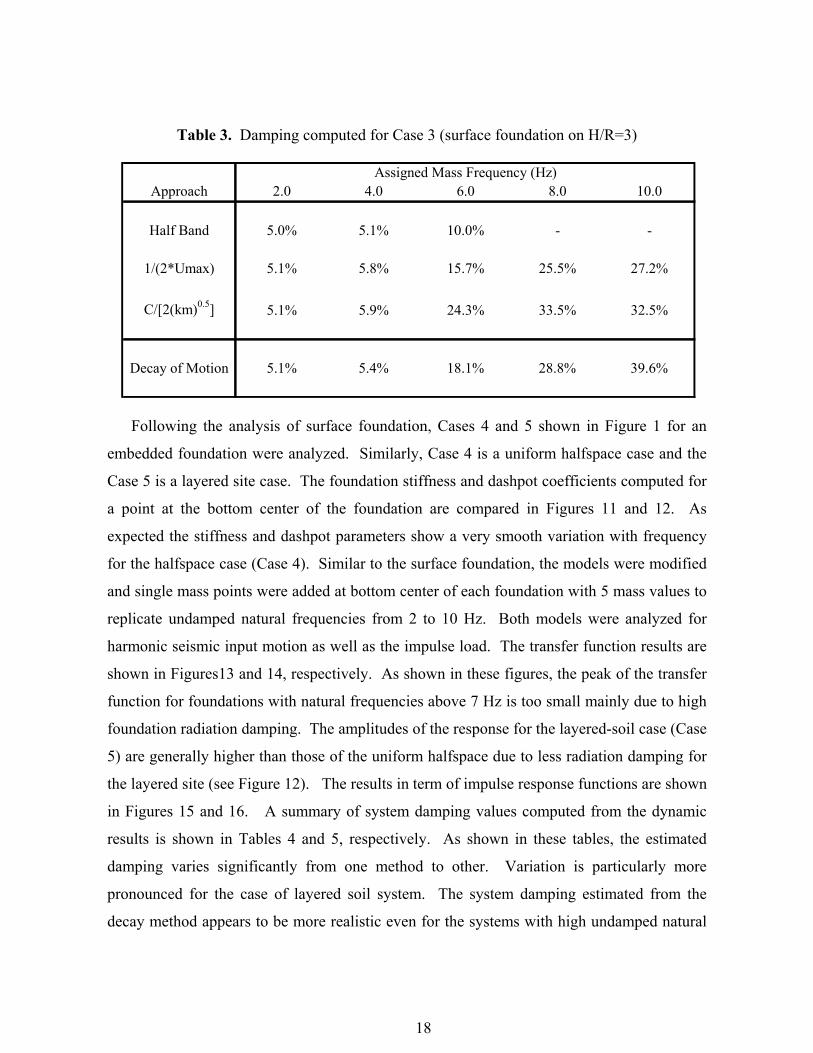
Table 3. Damping computed for Case 3 (surface foundation on H/R=3)

Following the analysis of surface foundation, Cases 4 and 5 shown in Figure 1 for an

embedded foundation were analyzed. Similarly, Case 4 is a uniform halfspace case and the

Case 5 is a layered site case. The foundation stiffness and dashpot coefficients computed for

a point at the bottom center of the foundation are compared in Figures 11 and 12. As

expected the stiffness and dashpot parameters show a very smooth variation with frequency

for the halfspace case (Case 4). Similar to the surface foundation, the models were modified

and single mass points were added at bottom center of each foundation with 5 mass values to

replicate undamped natural frequencies from 2 to 10 Hz. Both models were analyzed for

harmonic seismic input motion as well as the impulse load. The transfer function results are

shown in Figures13 and 14, respectively. As shown in these figures, the peak of the transfer

function for foundations with natural frequencies above 7 Hz is too small mainly due to high

foundation radiation damping. The amplitudes of the response for the layered-soil case (Case

5) are generally higher than those of the uniform halfspace due to less radiation damping for

the layered site (see Figure 12). The results in term of impulse response functions are shown

in Figures 15 and 16. A summary of system damping values computed from the dynamic

results is shown in Tables 4 and 5, respectively. As shown in these tables, the estimated

damping varies significantly from one method to other. Variation is particularly more

pronounced for the case of layered soil system. The system damping estimated from the

decay method appears to be more realistic even for the systems with high undamped natural

Approach 2.0 4.0 6.0 8.0 10.0

Half Band 5.0% 5.1% 10.0% - -

1/(2*Umax) 5.1% 5.8% 15.7% 25.5% 27.2%

C/[2(km)0.5] 5.1% 5.9% 24.3% 33.5% 32.5%

Decay of Motion 5.1% 5.4% 18.1% 28.8% 39.6%

Assigned Mass Frequency (Hz)

19

frequencies. The accuracy of this method is verified for a real size structure on a layered soil

site in the next section.

Figure 11. Horizontal foundation stiffness for Cases 4 and 5

Figure 12. Horizontal foundation dashpot coefficient for Cases 4 and 5

0.0E+00

1.0E+09

2.0E+09

3.0E+09

4.0E+09

5.0E+09

6.0E+09

7.0E+09

0 2 4 6 8 10 12 14 16 18 20

Frequency (Hz)

Stiff

ness

K (k

ips.

/ft.)

Kx - D/R=1 Embedded Fdn in Halfspace

Kx - D/R=1 Embedded Fdn in H/R=3 Layer

0.0E+00

2.0E+07

4.0E+07

6.0E+07

8.0E+07

1.0E+08

1.2E+08

1.4E+08

1.6E+08

0 2 4 6 8 10 12 14 16 18 20

Frequency (Hz)

Das

hpot

C (k

ips-

sec.

/ft.)

Cx - D/R=1 Embedded Fdn in HalfspaceCx - D/R=1 Embedded Fdn in H/R=3 Layer

20

Figure 13. Transfer function amplitude for Case 4 (embedded foundation in halfpace)

Figure 14. Transfer function amplitude for Case 5 (embedded foundation in layered soil)

0

0.5

1

1.5

2

2.5

3

3.5

0 2 4 6 8 10 12 14 16 18 20

Frequency (Hz)

Am

plitu

de o

f Tra

nsfe

r Fun

ctio

n

With 2Hz Mass

With 4Hz Mass

With 6Hz Mass

With 8Hz Mass

With 10Hz Mass

0

1

2

3

4

5

6

7

8

9

10

0 2 4 6 8 10 12 14 16 18 20

Frequency (Hz)

Am

plitu

de o

f Tra

nsfe

r Fun

ctio

n

With 2Hz Mass

With 4Hz Mass

With 6Hz Mass

With 8Hz Mass

With 10Hz mass

21

Figure 15. Impulse response functions for Case 4 (embedded foundation in halfpace)

Figure 16. Impulse response functions for Case 5 (embedded foundation in layered soil)

-0.4

-0.2

0

0.2

0.4

0.6

0.8

1

1.2

0.5 0.6 0.7 0.8 0.9 1 1.1 1.2 1.3 1.4 1.5 1.6 1.7 1.8 1.9 2

Time (second)

Impu

lse

Res

pons

e, U

2Hz Mass

4Hz Mass

6Hz Mass

8Hz Mass

10H

-0.6

-0.4

-0.2

0

0.2

0.4

0.6

0.8

1

1.2

0.5 0.6 0.7 0.8 0.9 1 1.1 1.2 1.3 1.4 1.5 1.6 1.7 1.8 1.9 2

Time (second)

Impu

lse

Res

pons

e, U

2Hz Mass

4Hz Mass

6Hz Mass

8Hz Mass

10H

22

Table 4. Damping computed for Case 4 (embedded foundation in halfpace)

Table 5. Damping computed for Case 5 (embedded foundation in layered soil)

CASE STUDY

In order to evaluate the effectiveness of the system damping obtained from the impulse

load method, a dynamic model of a vitrification structure was analyzed. The structure is a

concrete shear wall building with a foundation dimension of 322 ft by 253 ft. The major

floors in the building are located at Elev. –21 (basetmat), .0, 13, 36, 57 and 86 ft. The SASSI

model of the building is shown in Figure 17. Part of the building from ground surface (Elev.

.0 ft) to the bottom of the foundation (Elev. –21 ft) was modeled by finite elements and the

superstructure was modeled by a beam stick model. This is modeled to include the

foundation Frequency (Hz) Approach 2.0 4.0 6.0 8.0 10.0

Half Band 5.0% 5.1% 11.7% - -

1/(2*Umax) 5.3% 6.8% 23.4% 37.1% 43.9%

C/[2*(km) 0.5 ] 5.2% 6.3% 33.2% 61.5% 78.4%

Decay of Motion 5.1% 4.9% 18.6% 25.7% 28.7%

Foundation Frequency (Hz)

Approach 2.0 4.0 6.0 8.0 10.0

Half Band 16.5% 29.8% 61.8% - -

1/(2*Umax) 15.2% 24.2% 33.3% 41.3% 46.7%

C/[2*(km) 0.5 ] 15.6% 25.6% 37.3% 49.7% 62.3%

Decay of Motion 15.6% 24.8% 35.6% 43.6% 45.2%

23

embedment effect on SSI responses. However to simplify the analysis for this paper, the

ground surface was lowered to Elev. –21 ft thus eliminating the foundation embedment. The

fundamental fixed base structural modal frequency of the building in the East-West direction

is 12 Hz with 70% of the total mass. The stick model is a 3D model and includes eccentricity

of the shear and mass centers. A detailed view of the 3D model is shown in Figure 18.

Figure 17. SASSI Hybrid model of the vitrification building

X

Y

Z

Elev.

0

-21

North5

20

1

24

Figure 18. Stick model of the vitrification building

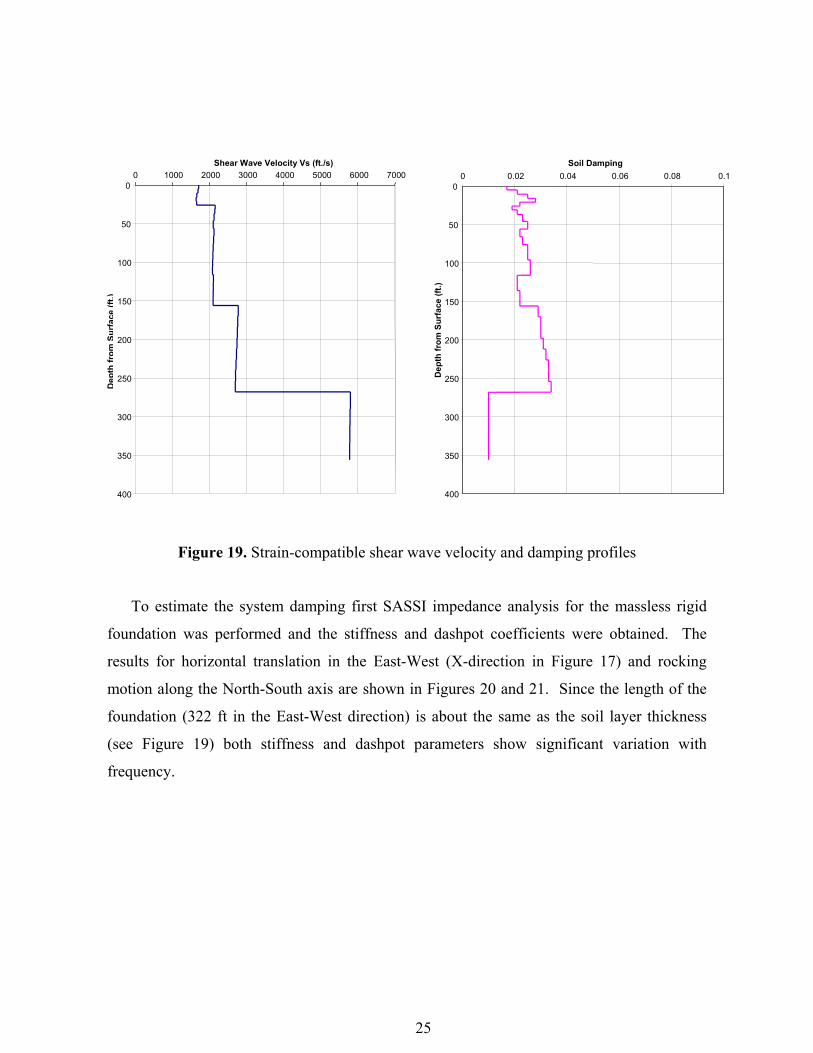
The site consists of very dense layers of sand and gravel with a total thickness of about

300 ft underlain by rigid rock. The strain-compatible shear wave velocity and damping

values obtained from free-field SHAKE (Schnabel et al, 1972) analysis are shown in Figure

19. The soils material damping ranges from 2% to 4% depending on the depth of the soil

layer.

Z

Y North

NORTH-SOUTH (Y)

Z

X EastYX

EAST-WEST (X)

EL. 86'

EL. 57'

EL. 36'

EL. 13'

EL. 0'

EL.-21'

ELEVATION ELEVATION

2.46

1.15

1.12

1.08

1.04

1.00

3.45

1.32

1.23

1.14

1.09

1.00

Dynamic 3D Stick Model

Notes: 1. Foundation Mat at El. -21. 2. Impulse loading time histories are applied on lumped

mass points. Numbers shown next to the arrows are relative magnitudes proportional to max. acceleration

values.

25

Figure 19. Strain-compatible shear wave velocity and damping profiles

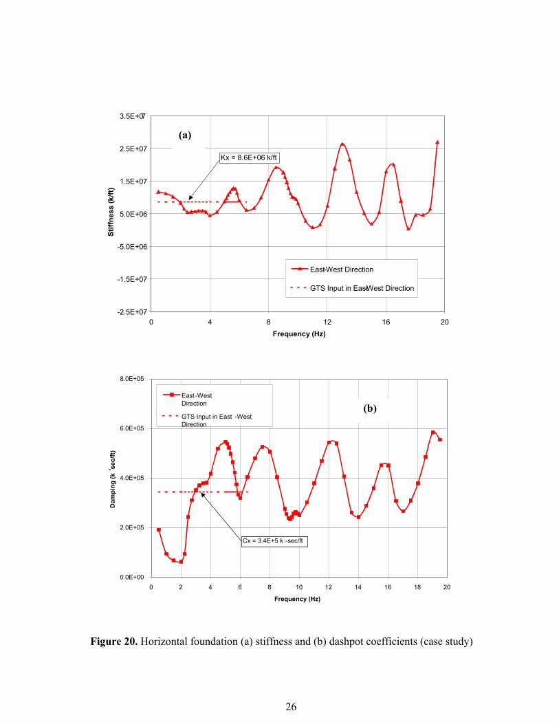
To estimate the system damping first SASSI impedance analysis for the massless rigid

foundation was performed and the stiffness and dashpot coefficients were obtained. The

results for horizontal translation in the East-West (X-direction in Figure 17) and rocking

motion along the North-South axis are shown in Figures 20 and 21. Since the length of the

foundation (322 ft in the East-West direction) is about the same as the soil layer thickness

(see Figure 19) both stiffness and dashpot parameters show significant variation with

frequency.

0

50

100

150

200

250

300

350

400

0 1000 2000 3000 4000 5000 6000 7000Shear Wave Velocity Vs (ft./s)

Dep

thfr

omSu

rfac

e(ft

.)

0

50

100

150

200

250

300

350

400

0 0.02 0.04 0.06 0.08 0.1Soil Damping

Dep

th fr

om S

urfa

ce (f

t.)

26

Figure 20. Horizontal foundation (a) stiffness and (b) dashpot coefficients (case study)

- 2.5E+07

- 1.5E+07

- 5.0E+06

5.0E+06

1.5E+07

2.5E+07

3.5E+0 7

0 4 8 12 16 20 Frequency (Hz)

Stiff

ness

(k/ft

)

East-West Direction

GTS Input in East-West Direction

Kx = 8.6E+06 k/ft

(a)

0.0E+00

2.0E+05

4.0E+05

6.0E+05

8.0E+05

0 2 4 6 8 10 12 14 16 18 20

Frequency (Hz)

Dam

ping

(k - se

c/ft)

East - West Direction GTS Input in East -West Direction

Cx = 3.4E+5 k -sec/ft

(b)

27

Figure 21. Rocking foundation (a) stiffness and (b) dashpot coefficients (case study)

-4.0E+11

-2.0E+11

0.0E+00

2.0E+11

4.0E+11

6.0E+11

0 4 8 12 16 20

Frequency (Hz)

Stiff

ness

(k-ft

/ ra

d)

About N-S Axis

GTS Input About N-S Axis

Kxx = 1.6E+11 k-ft/rad

0.0E+00

3.0E+09

6.0E+09

9.0E+09

1.2E+10

1.5E+10

0 4 8 12 16 20

Frequency (Hz)

Dam

ping

(k-s

ec-ft

/ ra

d)

About N-S Axis

GTS Input About N-S Axis

Cxx = 6.6E+08 k-sec-ft / rad

(a)

(b)

28

Following the impedance analysis, SSI analysis of the building was performed using

SASSI. The result in terms of amplitude of the total acceleration transfer function is shown

in Figure 22. As shown in this figure, the response is controlled by several modes of

vibration as evident by the numerous peaks in the transfer function plot. This is a typical

response of a multi-story structure on a layered soil system. The peak values are each

associated with the foundation stiffness and dashpot that also change with frequency. As

shown in Figure 22, it is very difficult to select a particular peak response to use as a basis for

obtaining the total system damping. A wrong choice for the peak response amounts to an

erroneous system damping.

Figure 22. Transfer function amplitude of the node at Elevation 58 ft (SASSI)

To estimate the system damping, the SASSI model (see Figure 17) was subjected to

impulse load at all mass points in the model. The time history of the impulse load is the same

one shown in Figure 2. However, the amplitude of the impulse load was adjusted depending

on the dynamic response of the mass points in the model. The amplitudes are proportional to

0

0.5

1

1.5

2

2.5

0 2 4 6 8 10 12 14 16 18 20Frequency (Hz)

Am

plitu

de

29

the maximum acceleration responses of the mass points from seismic analysis of the model.

The scale factors for impulse load for each of the mass points are shown in Figure 18. The

scale factors replicate the similar mode of vibration that is consistent with the maximum

response of the mass point at Elev. 57 ft. The impulse response function for the mass point at

Elev. 57 ft is shown in Figure 23. The response decays with a rate showing a system

damping of nearly 20%.

Figure 23. Impulse response function for the node at Elevation 58 ft (SASSI)

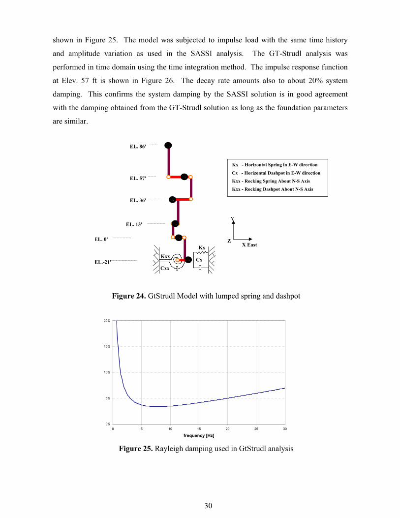
To verify the accuracy of the system damping, the analysis of the structure was repeated

using the GT-Strudl computer program (Georgia Tech. 2000). The GT-Strudl model is a

beam stick model as shown in Figure 24. The SASSI model and the GtStrudl model have the

same dynamic fixed base properties. The GT-Strudl model includes the stiffness and

dashpots constants in the horizontal and rocking directions at the base of the model. The

constants are the average values over a limited frequency range obtained from SASSI

impedance analysis (see Figures 20 and 21). The material damping in the structure was

modeled by Raleigh damping. The Rayleigh damping was constrained to 5% at 3 and 20 Hz

to cover the frequencies of the structure. The Rayleigh damping variation with frequency is

-0.6

-0.4

-0.2

0

0.2

0.4

0.6

0.8

1

0.5 1 1.5 2 2.5 3 3.5

Time (sec)

Impu

lse

Res

pons

e , U

El. 57'

Decay Fitting β = 19.6%

30

shown in Figure 25. The model was subjected to impulse load with the same time history

and amplitude variation as used in the SASSI analysis. The GT-Strudl analysis was

performed in time domain using the time integration method. The impulse response function

at Elev. 57 ft is shown in Figure 26. The decay rate amounts also to about 20% system

damping. This confirms the system damping by the SASSI solution is in good agreement

with the damping obtained from the GT-Strudl solution as long as the foundation parameters

are similar.

Figure 24. GtStrudl Model with lumped spring and dashpot

Figure 25. Rayleigh damping used in GtStrudl analysis

Kx

CxKxx

Cxx

Y

X EastZ

EL. 86'

EL. 57'

EL. 36'

EL. 13'

EL. 0'

EL.-21'

Kx - Horizontal Spring in E-W direction

Cx - Horizontal Dashpot in E-W direction

Kxx - Rocking Spring About N-S Axis

Kxx - Rocking Dashpot About N-S Axis

0%

5%

10%

15%

20%

0 5 10 15 20 25 30

frequency [Hz]

31

Figure 26. Impulse response function for the node at Elevation 58 ft (GtStrudl)

To compare the seismic response of the structure, both models were analyzed using the

acceleration time history of design motion as input. The results in terms of acceleration

response spectra at Elev. 57 ft are compared in Figure 27. As shown in this figure, the input

motion amplifies in the structure significantly yet a reasonably good agreement can be

obtained between the two solutions.

This case study also shows that by applying an impulse load on a SSI system and

developing the impulse response function one can effectively obtain a realistic estimate of the

total system damping.

-0.6

-0.4

-0.2

0

0.2

0.4

0.6

0.8

0.5 1 1.5 2 2.5 3 3.5

Time (sec)

Impu

lse

Res

pons

e, U

El. 57'

Decay Fitting

β = 20.8%

32

Figure 27. Comparison of acceleration response spectra at Elevation 58 ft

SUMMARY

The simple methods currently available to estimate system damping from dynamic

structural responses often fail to predict reasonable results for soil-structure systems due to

frequency dependency of the foundation stiffness and dashpot parameters and the complex

participation of the SSI and structural modes of vibration in the total response. These

methods include the half-bandwidth method, the inverse of the peak and the damping ratio

method. In this paper it has been shown that the response from an impulse load applied to

the SSI model yields an accurate estimate of system damping while including the effects of

material damping, radiation damping as well as composite effects of numerous structural and

SSI modes to the dynamic response of the interest. The damping computed may be used to

evaluate SSI effects and for input for other types of analysis such as nonlinear time history

analysis.

REFERENCES

Clough, R. W., Penzien, J. (1993), “Dynamic of Structures”, 2nd edition, McGraw Hill.

Chopra, A. K. (1995), “Dynamic of Structures”, Prentice Hall.

0.00

0.50

1.00

1.50

2.00

0.1 1 10 100

Frequency (Hz)

Spec

tral

Acc

eler

atio

n (g

) SASSI Hybrid Model, at El. 57'

GTStrudl Stick Model, at El. 57'

Input Motion

33

Lysmer, J., Ostadan, F., Chin, C. (1999), “SASSI2000- System for Analysis of Soil-Structure

Interaction”, University of California, Berkeley, California.

NUREG/CR-1780 (1980), “Soil-Structure Interaction: The Status of Current Analysis Methods and

Research”, Seismic Safety Margins Research Program, UCRL 53011.

Georgia Tech. (2000). “GT-STRUDL - Integrated CAE System for Structural Engineering Analysis

and Design, Version 25.0”, Georgia Tech Research Corporation, Atlanta, Georgia.

Schnabel, P. B.; Lysmer, J.; Seed, H. B. (1972), “SHAKE-A Computer Program for Earthquake

Response Analysis of Horizontally Layered Sites,” Report No. EERC 72-12, Earthquake

Engineering Research Center, UCB, December.