Estimating the Parameter Risk of a Loss Ratio … · 114 CASUALTY ACTUARIAL SOCIETY VOLUME 9/ISSUE 1 Estimating the Parameter Risk of a Loss Ratio Distribution—Revisited by Avraham

114 CASUALTY ACTUARIAL SOCIETY VOLUME 9/ISSUE 1

Estimating the Parameter Risk of a Loss Ratio Distribution—Revisited

by Avraham Adler

ABSTRACT

When building statistical models to help estimate future results,

actuaries need to be aware that not only is there uncertainty

inherent in random events (process risk), there is also uncertainty

inherent in using a finite sample to parameterize the models

(parameter risk). This paper revisits Van Kampen (2003) in rep-

licating its bootstrap method and compares it with measures of

parameter uncertainty developed using maximum likelihood

estimation and Bayesian MCMC analysis.

KEYWORDS

Parameter risk, bootstrap, maximum likelihood, Bayesian MCMC, JAGS, Stan, R, approximate Bayesian computation


VOLUME 9/ISSUE 1 CASUALTY ACTUARIAL SOCIETY 115

1. Introduction

Actuaries constantly build models. One of the beau-ties of mathematics is that it allows us to take ran-dom real-world phenomena, build a representation in the language of mathematics, and apply various tools allowing reasonable, and often surprisingly accu-rate, predictions about future phenomena. Of course, these models are just that—models, estimates of event behavior. If all real phenomena were perfectly pre-dictable the universe would be a rather dull place.

Actuarially speaking, “risk” has a specific defini-tion: it is the potential for future events to deviate from their expectation (Actuarial Standards Board 2012). There are many reasons why this could occur. The most basic reason is simply that such events are random events. The very process which generates the event has inherent uncertainty. Even if the model were perfectly specified, the stochastic nature of the process prevents absolute foreknowledge. In actu-arial terminology this is called process risk. Another reason why events may differ from their expectation is that the expectation itself is somehow imperfect. The error arising from an incorrect framework speci-fication, e.g., a lognormal distribution instead of a gamma, is called model risk. A third reason for devi-ation from expectation is that since the data used to select parameters for the model is inherently finite, the parameter estimators based on this sample may not be the perfect point estimates for the true under-lying parameters. This source of risk is what is usu-ally referred to as parameter risk. Sometimes, the more precise term finite-sample parameter risk is used to distinguish it from a separate cause of param-eter risk: the possibility that parameters may change over time. This paper will focus on finite-sample parameter risk, and, for convenience, will use the term “parameter risk.” An introduction to these and other examples of potential bias and distortion can be found in Venter and Sahasrabuddhe (2012).

In the remainder of this paper, Section 2 will intro-duce Van Kampen’s data and bootstrapping method, Section 3 will discuss parameter risk estimation using maximum likelihood, Section 4 will use Bayesian

Markov Chain Monte Carlo (MCMC) to estimate the parameter risk, and Section 5 will compare the methods and results. The appendix will bring much of the source code used to fit the models and gen-erate this paper, which is predominantly performed using R (R Core Team 2014).1 Bringing actual code, instead of only results, is intended to enhance trans-parency and reproducibility. While basic knowledge of R and MCMC techniques is not required, it would help the reader interested in reproducing or extending the results.

2. Bootstrapping

Van Kampen discusses estimating both a ground up loss ratio and the expected loss for an aggregate stop loss reinsurance contract. Table 1 reproduces the data, a sequence of historical ground-up loss ratios

1The paper, formulæ, R output, and images have been generated using knitr (Xie 2013).

Table 1. Loss ratio distribution

YearLoss Ratio

LN(Loss Ratio)a

Agg Stop LR

1 0.5841 -0.5376 0.0000

2 0.6448 -0.4388 0.0000

3 0.6735 -0.3953 0.0000

4 0.5265 -0.6415 0.0000

5 0.5841 -0.5376 0.0000

6 0.6448 -0.4388 0.0000

7 0.7835 -0.2440 0.0250

8 0.7055 -0.3488 0.0000

9 0.6197 -0.4786 0.0000

10 0.6448 -0.4388 0.0000

Empirical Mean 0.6411 -0.4500 (µ) 0.0025

Empirical StDev 0.0712 0.1100 (s) 0.00791

Empirical Skew 0.5003

Fitted LRb 0.6415 0.00235

Empirical Loss on Line 0.1000

Fitted Loss on Line 0.0939aFor this table, the logged values in Van Kampen’s Exhibit 1 were taken as accurate and the loss ratios displayed in that table are assumed to be rounded.bThe expected loss ratios are based on the empirical µ and s parameters.

Variance Advancing the Science of Risk


In 2003, this procedure took around 8 hours; in 2014, after some optimization described in Section 7.1.2, it took a little under two minutes. Hardware and soft-ware advances in the intervening years have created an over 270 times increase in speed! Taking advantage, a more finely-grained grid was investigated. Using the results of the original bootstrap to focus a new grid, a second procedure was run with µ ranging from -0.8 to -0.2 and s from 0.05 to 0.45, each moving in steps of 0.0025. Bootstrapping these 38,801 pairs took about 17 minutes on the same machine.

Unsurprisingly, the results shown in Table 2 are similar to those in the original paper. While recogniz-ing parameter risk is always important, it is more so when dealing with rare events. Even a small thick-ening of the tail of a distribution may make a sig-nificant difference in the expected results excess of a threshold. When parameter risk is contemplated with this data, there is almost no increase in the ground-up expected loss but a significant increase to the highly tail-sensitive excess layer. Note how the more fine-grained algorithm’s ground-up estimate is only slightly different from that of the original algorithm, but the aggregate stop loss ratio estimate is noticeably larger.

Visual inspection of data is always valuable (Anscombe 1973). When investigating parameter risk for two-parameter distributions, one useful tool is the contour plot—a two-dimensional projection of the three-dimensional surface of the joint distribu-tion of the parameters. Contour images in this paper will reflect the increase in probability of a given set of parameters by a brightening of the color as it shades from red to yellow.

and the corresponding experience to an aggregate stop loss cover of 2.5% excess of 72.5%.

The approach taken by Van Kampen is to make an initial estimate and then create random variates on a grid of parameters near that estimate. All parameters sets which are deemed “close” are marked and used to create a new weighted average expectation. The theory is that the observed data leading to the best estimate of the parameters may have actually come from a different set of parameters. Allowing for the use of many sets of parameters and weighting them by some measure of probability that they were the “true” source will reflect parameter uncertainty. The bootstrap algorithm itself is:

1. Generate a possible µ and s for the lognormal.

2. Generate 10,000 observations of 10-year blocks.

3. Compare the simulated mean, standard deviation, and skew of each of the simulated blocks with those of the original data. If any 10-year block has all three check values sufficiently close to the best estimate, the parameter set is marked as viable.

4. Assign a weight to each viable parameter set based on the number of its blocks found to be close.

5. Calculate a weighted average expected ground up and aggregate stop loss ratio using all the viable parameter sets to arrive at a final point esti-mate which now includes the impact of parameter uncertainty.

Based on Van Kampen’s description, the search grids was set as the intersections of 51 data points for µ in the range -1.549–0.226 (50 equispaced points and the addition of -0.45) and 79 equispaced data points for s in the range 0.0055–0.4345 for a total of 4,029 parameter sets. For each of these sets, 100,000 lognormal variates were generated and placed into a 10,000 by 10 matrix. A viable parameter set was selected based on the same measure of “closeness” used in the original paper (pp. 187–188). For each viable set, the expected ground-up and expected aggregate loss ratios were calculated, and the over-all estimate is a frequency-weighted average of the viable results.

Table 2. Bootstrap parameter risk results

Statistic Original Adjusted Change

Original Algorithm

Ground Up LR 0.6415 0.6436 0.00328

Agg. Stop LR 0.00235 0.00318 0.3554

Fine-grain Algorithm

Ground Up LR 0.6415 0.644 0.00395

Agg. Stop LR 0.00235 0.00336 0.4323



the Hessian matrix at the point of convergence can be calculated and its inverse used to estimate param-eter variances and covariances. An intuitive explana-tion for the relationship between the curvature of the log-likelihood and parameter uncertainty is as fol-lows. The estimation process looks for a minimum for the negative log-likelihood by following the joint log-likelihood’s (hyper)surface. The Hessian matrix describes the curvature of a multivariate function, in this case, the log-likelihood. In a bivariate case, imagine the procedure as a marble rolling around on the log-likelihood surface. Compare the two surfaces in Figure 2. If the gradient at the found minimum is low, that would represent a shallow depression and it would be easy to “jostle” the marble to a different point nearby. This represents significant parameter uncertainty, as the true point could easily have been elsewhere. Conversely, if the gradient is high, the depression is deep and it would be difficult to move the marble. This implies the convergence to the found point is strong, and there is less parameter uncertainty.

Contour plots of the joint empirical distribution of the close pairs of µ and s for the original and fine-grained algorithms are plotted in Figure 1.2 The skew of the distribution is clear.

3. Maximum likelihood

3.1. Introduction

One of the most used tools in the actuarial toolbox is maximum likelihood estimation (MLE). Among the properties of MLE is that the estimated parame-ters have asymptotic normality—under general con-ditions, as the sample size increases, the distribution of the maximum likelihood estimate of the parame-ters tends to the multivariate normal with covariance matrix equal to the inverse of the Fisher information matrix (Klugman, Panjer, and Willmot 1998, §2.5.1). Assuming this normality, when performing MLE,

2Contour plots generated using ggplot2 (Wickham 2009).

Figure 1. Contour plots of bootstrap parameters

Fine-grainOriginal

-0.8

-0.6

-0.4

-0.2

0.05 0.15 0.200.10 0.25σ

µ

30

60

90

120level

-0.8

-0.6

-0.4

-0.2

0.05 0.15 0.25σ

µ

25

50

75

100

125level

0.10 0.20

Contour plots of the empirical distribution of the Van Kampen bootstrap procedure. The skew can be observed by noting that the area of highest probability, the yellow zone, is horizontally offset to the left of the minor axis of the ellipse, thus the right tail is larger than the left tail.



at times, to trim the mean to prevent edge cases from dominating the results. In all the MLE instances below, the mean is trimmed by 0.1%. As 1,000,000 samples are drawn for each of the MLE stochastic simulations, this means that the top and bottom 500 observations are removed and the statistics are calcu-lated on the remaining 999,000 samples.

Continuing with the lognormal assumption, the results of solving for the parameters using MLE on the sample data are shown in Table 3.3 A stochastic simulation was used to estimate the effects of param-eter risk. Pairs of correlated µ and s parameters were generated, each of which was then used for a sto-chastic lognormal draw of the observed ground-up loss ratio.4 Given the drawn ground-up loss ratio, the resulting aggregate stop loss (ASL) ratio was simply the loss in a layer 2.5% excess of 72.5%. All means are trimmed as described above.

The simulated results, shown in Table 4, indicate almost no change from the original. This is more

3.2. Estimation and simulation

Given the assumption of normality, once a set of parameters is estimated by maximum likelihood, the Hessian can be used to generate the parameter variance-covariance matrix. Using these parameter means and covariances, sets of correlated param-eters can be generated using a multivariate normal distribution—the asymptotic limiting distribution of maximum likelihood estimators. These correlated parameter sets are then used to draw one observation each from the distribution of interest. The collected observations now represent a sample with explicit recognition of parameter uncertainty, as the param-eters generating the observations themselves were treated as random variables. Care needs to be taken, however, as the multivariate normal will sometimes generate parameters which themselves are illegal for the distribution in question. For example, the s of a lognormal distribution must be greater than 0, yet a multivariate normal may generate a value less than 0. Similarly, a value very close to 0 may be gener-ated when its reciprocal is needed, resulting in an astronomical value. There are a few ways to address this problem, the simplest being to ignore generated values which cause illegal results. It is also prudent,

Figure 2. Representative likelihood surfaces

x y

Likelihood

x y

LikelihoodSteep CurvatureLow Uncertainty

Shallow CurvatureHigh Uncertainty

3Optimization performed using the nloptr (Ypma 2014) interface to the NLOPT library (Johnson 2010).4Multivariate normal simulation performed using the mvtnorm package for R (Genz et al. 2014).



eter gamma and Weibull distributions and the three parameter Burr and inverse Burr distributions.6 Infor-mation criteria, such as the Akaike Information Crite-ria (AICc)7 are often used to compare models. When using information criteria, two points must be kept in mind. First, the criteria can only be compared between models based on the exact same data. Second, it is not the magnitude of the value, but the difference between the lowest value and all the others, which is important (Burnham and Anderson 2002, chap. 2). When used appropriately, accepted rules of thumb are that a difference of 0–2 implies model similar-ity, a difference of 4–7 shows that the model with the higher value has little support with respect to the model with the lower value, and larger differences imply that the higher-valued model should really not be considered at all (Burnham and Anderson 2002, pp. 70–71; Spiegelhalter et al. 2002).

The best fits, as shown in Table 5, are the log normal and the gamma, with the Weibull being acceptable. The Burr and inverse Burr are each more than 4 away from the minimum, showing little support. Nevertheless, it is instructive to see the difference between using a better model and a worse one. Don’t all the models arise from reasonable analyses and the same processes? The goodness-of-fit measures don’t really look that bad, do they? The AICc difference not even 5, right? What if the AICc’s were 18,204.3 and 18,208.9, wouldn’t that be “close enough”? These are questions the actuary may receive, if not ask of him or herself. Often, actuaries are exposed to “good” results and do not always have a yardstick for “bad” ones. Being able to recognize when processes

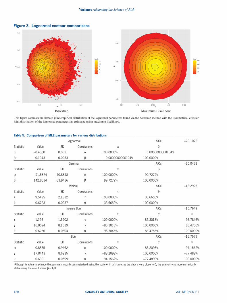
easily understood visually. Figure 3 compares re- scaled bootstrap and MLE-based contour plots, and also has explicitly plotted density isolines. When the plotted ranges are no longer restricted to the ranges in the original paper, the plot clearly contrasts the symmetrical uncorrelated nature of the MLE-based parameters with the skewed bootstrapped parameters. The isolines, along which each parameter set is equi-probable, further demonstrate the circular nature of the MLE-based results. This is predominantly due to the parameters being uncorrelated with each other.5 When pairs of multivariate normal variables are uncor-related (or r = 0 in the bivariate case), that is sufficient to imply their independence (Melnick and Tenenbein 1982). Therefore, under the lognormal assumption, since µ and s are independent and uncorrelated, any pair of parameters which would result in a loss above the overall expectation is balanced by one equally probable which would cause an equally lower loss. When the parameters exhibit correlation, and possi-bly even more strongly in a skewed distribution, it is possible to obtain an observation which cannot be balanced by its equal and opposite “across the circle of probability.”

3.3. Other distributions

To investigate how correlation between the param-eters may affect the results, the MLE fitting was done using other distributional families: the two param-

Table 4. Lognormal MLE stochastic results


Ground Up LR 0.6415 0.6415 -0.0000404

Agg. Stop LR 0.00235 0.0023 -0.0197

Table 3. Lognormal MLE parameters

Statistic Value SD Correlations µ s

µ -0.4500 0.0330 µ 100.0000% 0.0000000000104%

s 0.1043 0.0233 s 0.0000000000104% 100.0000%

AICc -20.1072

5This is actually a consequence of a known property of the normal dis-tribution in that its sample mean and sample variance are independent (Geary 1936).

6Unless otherwise noted, all distributions follow the parameterization in Appendix A of Klugman, Panjer, and Willmot (1998).7The actual criterion being used is the Akaike Information Criteria with small-sample bias correction, thus the second “c” (Burnham and Anderson 2002, p. 66).



-0.55

-0.50

-0.45

-0.40

-0.35

0.10 0.15 0.20σ

µ

25

50

75

100

125level

-0.52

-0.48

-0.44

-0.40

0.050 0.075 0.100 0.125 0.150σ

µ

50

100

150

200level

Bootstrap Maximum Likelihood

This figure contrasts the skewed joint empirical distribution of the lognormal parameters found via the bootstrap method with the symmetrical circular joint distribution of the lognormal parameters as estimated using maximum likelihood.

Figure 3. Lognormal contour comparisons

Table 5. Comparison of MLE parameters for various distributions

Lognormal AICc -20.1072

Statistic Value SD Correlations a b

a -0.4500 0.033 a 100.0000% 0.0000000000104%

ba 0.1043 0.0233 b 0.0000000000104% 100.0000%

Gamma AICc -20.0431

Statistic Value SD Correlations a b

a 91.5874 40.8848 a 100.0000% 99.7272%

ba 142.8514 63.9436 b 99.7272% 100.0000%

Weibull AICc -18.2925

Statistic Value SD Correlations t q

t 9.5425 2.1812 t 100.0000% 33.6650%

q 0.6723 0.0237 q 33.6650% 100.0000%

Inverse Burr AICc -15.7649

Statistic Value SD Correlations t g q

t 1.196 1.5902 t 100.0000% -85.3018% -96.7846%

g 16.0524 8.1019 g -85.3018% 100.0000% 83.4756%

q 0.6266 0.0804 q -96.7846% 83.4756% 100.0000%

Burr AICc -15.7579

Statistic Value SD Correlations a g q

a 0.8835 0.9462 a 100.0000% -83.2098% 94.1562%

g 17.8443 8.6235 g -83.2098% 100.0000% -77.489%

q 0.6301 0.0599 q 94.1562% -77.4890% 100.0000%aAlthough in actuarial science the gamma is usually parameterized using the scale q, in this case, as the data is very close to 0, the analysis was more numerically stable using the rate b where b = 1/q.



est contributions actuaries make is to understand, and provide the context for, the statistics which will be used. Yes, 10196% may be one observation out of one million that can mathematically arise from a ran-dom draw of underlying inverse Burr parameters, but it should it be considered a possible event? Certainly not! Therefore, not only were illegal parameters sets removed, but a judgment-based reasonability cap for the ground-up loss ratios of 300% was implemented as well. For the inverse Burr, there were 234,511 parameter sets which were removed from the analy-sis due to being invalid or in excess of the cap. For the Burr, there were 187,233 such observations.

Table 6 shows the results of the stochastic simula-tions for these distributions, and the inferences made using all, and then the 765,489 and 812,767 remaining reasonable, observations respectively. The “small” difference in the AICc of the parameters manifests as a very significant difference in the modeled results including parameter uncertainty. The results for the

fail and how that can affect analyses is an important part of actuarial analysis. Therefore, the stochastic parameter uncertainty process was applied to each of these models as well to provide a sense of poor performance.

Using the fitted parameter means and covariance matrix for each distribution, one million correlated observations were generated. Since using a multi-variate normal to generate observations makes it possible to obtain negative values, the same filtering and trimming used for the lognormal were used for these distributions as well. Unfortunately, even with the trimming, the multivariate normal generated too many unacceptable parameter sets at times. This was due not only to “illegal” parameter sets but also to parameter sets which generated unreasonable results, such as ground-up loss ratios greater than 10196% for the inverse Burr. This further highlights the need for actuarial judgment, which should always temper raw algorithmic output, in any analysis. One of the larg-

Table 6. Comparison of MLE-based parameter uncertainty for various distribution


Lognormal

Ground Up Loss Ratio 0.6415 0.6415 -0.0000404

Agg. Stop Loss Ratio 0.00235 0.0023 -0.0197

Gamma

Ground Up Loss Ratio 0.6415 0.6430 0.00225

Agg. Stop Loss Ratio 0.00235 0.0027 0.1499

Weibull



Inverse Burr



Inverse Burr—Valid Results



Burr



Burr—Valid Results





three distributions with acceptable goodness-of-fits, the lognormal continues to show little effect from parameter risk, the gamma now shows almost none as well, and the aggregate stop loss under the Weibull also demonstrates a smaller effect.

4. Bayesian analysis

4.1. Introduction

A third way to incorporate parameter risk is through a Bayesian model using Markov Chain Monte Carlo (MCMC) techniques. Roughly speaking, the Bayes-ian approach is that there exists an a priori estimate of the distribution of the parameters, which, when convoluted with the data, allows for the calculation of an a posteriori distribution of those parameters (Gelman et al. 2014, Chap. 1.3). The Bayesian model can be made even more sophisticated through explicit recognition of parameter dependency through hyper-parameters. A model in which there exists a hierar-chical structure of parameter dependency is called, understandably, a hierarchical model (Kruschke 2015, pp. 221–223). Creating a model with such structure allows the joint probability model to reflect potential dependencies between the parameters (Gelman et al. 2014 p. 101). Both simple and hierarchical models explicitly recognize parameter risk by generating a posterior distribution around the parameters. More-over, distributions of the statistics of interest, such as loss rations, can also be easily generated with explicit reflection of parameter risk.

While the Bayesian concept is relatively simple, for almost two centuries its application was difficult, as the convolution often required the calculation of integrals without nice analytic solutions. In the past few decades, advances in both algorithms and com-puter hardware have made these computations much simpler. The method used in this paper, MCMC, takes advantage of certain properties of Markov chains that allow it to converge to the posterior distribution without fully calculating some of the more difficult integrals. For more explanation, the interested reader is directed to Kruschke (2015, chap. 7) and Gelman et al. (2014, chap. 11).

three-parameter distributions, even when trimmed, are just plain ridiculous. Even among the models which only reflect “realistic” observations, the results seem extreme when compared to the distributions with acceptable AICc measures.

3.4. Estimation and simulation on a log scale

Another common way to prevent negative param-eters in a simulation is to reparameterize the distribu-tions so that the optimization solves for an extremum of the log of the parameters, and this value is then exponentiated for use in simulation. This transforma-tion also affects the shape of the joint distribution of the parameters in normal space, as parameters exhib-iting symmetry on a log scale will not be symmetric on a normal scale. Table 7 displays the results of the simulations including the effects of parameter uncer-tainty using parameters fitted on a log scale. For the

Table 7. Comparison of log scale MLE-based parameter uncertainty for various distribution


Lognormal



Gamma



Weibull



Inverse Burr



Inverse Burr—Valid Results



Burr



Burr—Valid Results





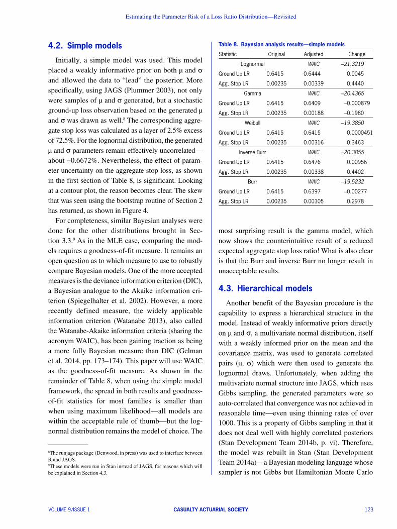
most surprising result is the gamma model, which now shows the counterintuitive result of a reduced expected aggregate stop loss ratio! What is also clear is that the Burr and inverse Burr no longer result in un acceptable results.

4.3. Hierarchical models

Another benefit of the Bayesian procedure is the capability to express a hierarchical structure in the model. Instead of weakly informative priors directly on µ and s, a multivariate normal distribution, itself with a weakly informed prior on the mean and the covariance matrix, was used to generate correlated pairs (µ, s) which were then used to generate the lognormal draws. Unfortunately, when adding the multivariate normal structure into JAGS, which uses Gibbs sampling, the generated parameters were so auto-correlated that convergence was not achieved in reasonable time—even using thinning rates of over 1000. This is a property of Gibbs sampling in that it does not deal well with highly correlated posteriors (Stan Development Team 2014b, p. vi). Therefore, the model was rebuilt in Stan (Stan Development Team 2014a)—a Bayesian modeling language whose sampler is not Gibbs but Hamiltonian Monte Carlo

4.2. Simple models

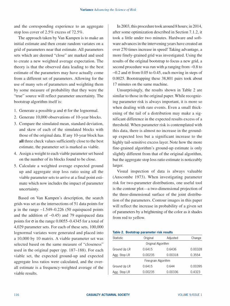
Initially, a simple model was used. This model placed a weakly informative prior on both µ and s and allowed the data to “lead” the posterior. More specifically, using JAGS (Plummer 2003), not only were samples of µ and s generated, but a stochastic ground-up loss observation based on the generated µ and s was drawn as well.8 The corresponding aggre-gate stop loss was calculated as a layer of 2.5% excess of 72.5%. For the lognormal distribution, the generated µ and s parameters remain effectively uncorrelated—about -0.6672%. Nevertheless, the effect of param-eter uncertainty on the aggregate stop loss, as shown in the first section of Table 8, is significant. Looking at a contour plot, the reason becomes clear. The skew that was seen using the bootstrap routine of Section 2 has returned, as shown in Figure 4.

For completeness, similar Bayesian analyses were done for the other distributions brought in Sec-tion 3.3.9 As in the MLE case, comparing the mod-els requires a goodness-of-fit measure. It remains an open question as to which measure to use to robustly compare Bayesian models. One of the more accepted measures is the deviance information criterion (DIC), a Bayesian analogue to the Akaike information cri-terion (Spiegelhalter et al. 2002). However, a more recently defined measure, the widely applicable infor mation criterion (Watanabe 2013), also called the Watanabe-Akaike information criteria (sharing the acronym WAIC), has been gaining traction as being a more fully Bayesian measure than DIC (Gelman et al. 2014, pp. 173–174). This paper will use WAIC as the goodness-of-fit measure. As shown in the remainder of Table 8, when using the simple model framework, the spread in both results and goodness-of-fit statistics for most families is smaller than when using maximum likelihood—all models are within the acceptable rule of thumb—but the log-normal distribution remains the model of choice. The

Table 8. Bayesian analysis results—simple models


Lognormal WAIC -21.3219

Ground Up LR 0.6415 0.6444 0.0045

Agg. Stop LR 0.00235 0.00339 0.4440

Gamma WAIC -20.4365

Ground Up LR 0.6415 0.6409 -0.000879

Agg. Stop LR 0.00235 0.00188 -0.1980

Weibull WAIC -19.3850

Ground Up LR 0.6415 0.6415 0.0000451

Agg. Stop LR 0.00235 0.00316 0.3463

Inverse Burr WAIC -20.3855

Ground Up LR 0.6415 0.6476 0.00956

Agg. Stop LR 0.00235 0.00338 0.4402

Burr WAIC -19.5232

Ground Up LR 0.6415 0.6397 -0.00277

Agg. Stop LR 0.00235 0.00305 0.2978

8The runjags package (Denwood, in press) was used to interface between R and JAGS.9These models were run in Stan instead of JAGS, for reasons which will be explained in Section 4.3.



Now, the effect of parameter risk much more in line with expectations—close to that of the hierarchical lognormal—and the goodness-of-fit measure is greatly improved and much closer to that of the lognormal. A comparison of the contour plots of the joint distribu-tions of the parameter pairs between the simple and hierarchical models is shown in Figure 5.

5. Comparison and conclusions

5.1. Comparisons

One of the first observations that can be made is that the bootstrap results appear very similar to the

(Gelman et al. 2014, 12.4–12.6).10 The No-U-Turn-Sampler used by Stan is much more robust to highly autocorrelated parameters (Hoffman and Gelman 2014). To provide reassurance that the model was built correctly, the non-hierarchical lognormal model was also programmed in Stan to compare the fitted results with those of JAGS.

The ability to expressly consider a hierarchical structure becomes more valuable when contemplat-ing the gamma distribution. The simple Bayesian gamma model showed the counter-intuitive reduced aggregate stop loss ratio. As the gamma parameters are extremely correlated with each other—99.7272% using maximum likelihood and 99.7251% in the sim-ple Bayesian model—it makes sense to consider a hierarchical Bayesian model to directly generate cor-related gamma parameters.

Table 9 shows that adding hierarchical hyperpriors to expressly model correlation between the log normal µ and s reduces the effect of parameter uncertainty in the aggregate stop loss for the lognormal distribution with almost no change to the goodness-of-fit as mea-sured by WAIC. Expressly modeling the correlation in the gamma distribution had a much larger effect.

-0.55

-0.50

-0.45

-0.40

-0.35

0.10 0.15 0.20σ

µ

25

50

75

100

125level

Bootstrap

-0.52

-0.48

-0.44

-0.40

0.050 0.1000.075 0.125 0.150σ

µ

50

100

150

200level

Maximum Likelihood

-0.50

-0.45

-0.40

0.09 0.12 0.15 0.18σ

µ

50

100

level

Bayesian

Three-way comparison of lognormal contours. The bootstrap- and Bayesian-based parameter distributions show very similar behavior and skew, unlike the circular results of the MLE-based process.

Figure 4. Lognormal contour comparisons showing presence or absence of skew

10The hierarchical structure of the lognormal model was investigated prior to the simple models of the other distributions, which explains why the remaining simple models in Section 4.2 were built in Stan instead of JAGS. The original lognormal JAGS model remains to demonstrate that both types of sampling converge to very similar results.

Table 9. Bayesian analysis results—hierarchical models


Lognormal Simple—JAGS WAIC -21.3219

Ground Up LR 0.6415 0.6444 0.0045

Agg. Stop LR 0.00235 0.00339 0.4440

Lognormal Simple—Stan WAIC -21.3237

Ground Up LR 0.6415 0.6443 0.00436

Agg. Stop LR 0.00235 0.00338 0.4379

Lognormal Hierarchical—Stan WAIC -21.4386

Ground Up LR 0.6415 0.6425 0.00156

Agg. Stop LR 0.00235 0.00296 0.2609

Gamma Hierarchical—Stan WAIC -21.3235

Ground Up LR 0.6415 0.6421 0.000882

Agg. Stop LR 0.00235 0.00294 0.2525



constrained to a symmetric ellipse centered on the area of highest density.

This near-identicality is not surprising. Van Kam-pen’s bootstrap is actually an example of Approxi-mate Bayesian Computation (ABC). Described in theory by Rubin (1984), and named by Beaumont, Zhang, and Balding (2002), ABC comprises methods where approximations to Bayesian posteriors are cal-

Bayesian results in both magnitude and distribution— especially with the simple model. Overlaying the contours of the distributed parameters, as shown in Figure 6, highlights the relationship between the methods. The area of highest density is shared by all three methods. However, while the Bayesian con-tours show the same skew and coverage as the boot-strap contours, the maximum likelihood contours are

HierarchicalSimple

Lognormal

-0.50

-0.45

-0.40

0.05 0.10 0.15σ

µ

40

80

120

160level

-0.50

-0.45

-0.40

0.05 0.10 0.15σ

µ

50

100

150

level

Gamma

0

100

200

300

0 100 20050 150β

α

0.00005

0.00010

0.00015

0.00020

0.00025

0.00030level

0

100

200

300

0 100 20050 150β

α

0.0001

0.0002

0.0003

0.0004

level

A comparison of the contour plots for the joint distribution of the parameter sets for the lognormal and gamma distributions under the simple and hierarchical models. The axes across model type for each distribution are the same. The lognormal shows almost no change, but the gamma shows a shift of the entire ellipse, and the areas of highest probability, towards the origin. Generating correlated pairs of α and β parameters, as opposed to each independently, has made a difference.

Figure 5. Simple vs. hierarchical contour plot comparison



(Beaumont, Zhang, and Balding 2002; Bornn et al. 2014); and 2) it allows for easier to expression and investigation of hierarchical relationships (Turner and Van Zandt 2014, pp. 6–7). Therefore, where an analytic expression of the needed likelihood(s) are not that difficult to calculate, it makes sense to use the fully Bayesian technique.

Figure 7 compares the joint distribution of the gen-erated parameter sets under MLE, log-space MLE, and the Bayesian framework for the two-parameter distributions. The joint distribution of the parameters generated by maximum likelihood methods are con-strained to a symmetric elliptical distribution. Even when solving for parameters in log-space, the result-ing normal space parameters are still mainly ellip-tical with some distortion. The Bayesian models, however, are not constrained to symmetric ellipticity.

This is even clearer for the three-parameter distri-butions. Figure 8 compares the parameter clouds of the distributions; each point representing a parameter triplet. The colored version of the clouds have fewer points than the monochrome versions, as they are composed only of the points which led to valid val-ues. For these plots, the brightness and color of the points reflect the magnitude of the resulting value; e.g., bright yellow triplets will have a correspond-ingly larger expected ground-up loss ratio than the dull red triplets.

There are two important takeaways from Figure 8. The first regards the structure of the clouds. The normal space MLE clouds are clearly constrained to be ellipsoids. The log-space MLE clouds break from that constraint but seem to be more “stretched” and “bent” ellipsoids than entirely different shapes. The Bayesian process, however, allows the data to determine the shape of the posterior distribution and results in strangely-shaped surfaces which expand to fill the parameter space. The inverse Burr traces a sheet that inhabits different sections of q and g space than the other two inverse Burr clouds. The Burr cloud is more a sheet with a small tail that extends down g space. The second takeaway is the relation-ship between parameter and value. In the normal ellip-soid it is difficult to see. In the log-space versions

culated by simulating outcomes based on parameters selected from their prior distributions, rejecting param-eter sets whose outcomes lie outside an accepted toler-ance, and estimating the posterior distribution based on the remaining “accepted” samples.11 This method circumvents the need to calculate any likelihood; all that is needed is the prior, summary statistics, and a tolerance. This is precisely what Van Kampen’s bootstrap does: sample from the uniform grid (prior on parameters), reject outcomes whose summary sta-tistics are not close (rejection outside tolerance), and calculate results based on weighted averages of the remaining samples (posterior estimation).

Nevertheless, the truly Bayesian procedure has at least two benefits: 1) studies have shown that given data sets allowing for true MCMC, the MCMC results are more accurate than those of rejection-based methods

-0.50

-0.45

-0.40

-0.35

0.05 0.150.10 0.20σ

µ

Bayes(Simple)

Bootstrap

MLE

This image shows the relationship between the joint distribution of the lognormal parameters estimated using the bootstrap method and the Bayesian method, as opposed to the MLE-based method. All three sets of isolines converge to the same mode. The red (Bayesian) and green (bootstrap) isolines, however, trace out the same area in the same way, although the red isolines are smoother. The blue (MLE) isolines tell a different story. They are constrained to a symmetrical unskewed ellipse, which shows more probability to the left of the mode, and less to the right.

Figure 6. Superimposed lognormal contour plots

11For a very clear, if informal, explanation and description of basic ABC, the interested reader is directed to Bååth (2014).



Looking at a summary of results, shown in Table 10, the Bayesian process allows the fit for each family to affect the ground-up loss ratio minimally yet show similar leveraged effects on the aggregate stop loss. Also, even the families with worse fits were not as unreasonable as they were using maximum likelihood. Another key difference is in identifying the “best”

it is somewhat clearer to see a relationship between the parameter triplet’s position and resulting mean value. However, the relationship between structure and value appear clearest in the Bayesian clouds. The inverse Burr’s expectation’s relationship with q is clearly seen. For the Burr, most of the parameter cloud is a thin sheet, yellow on one side and red on the other.

2.0

Normal Space Log-space Bayesian

Lognormal

-0.52

-0.48

-0.44

-0.40

0.05 0.10 0.15σ

µ

50

100

150

200level

-0.52

-0.48

-0.44

-0.40

0.05 0.10 0.15σ

µ

50

100

150

200level

-0.50

-0.45

-0.40

0.05 0.10 0.15σ

µ

50

100

150

level

Gamma

0

100

200

300

0 100 20015050β

α

0.0001

0.0002

0.0003

0.0004

0.0005level

0

100

200

300

0 15010050 200β

α

0.0001

0.0002

0.0003

0.0004

0.0005

level

0

100

200

300

0 100 20050 150β

α

0.0001

0.0002

0.0003

0.0004

level

Weibull

0.62

0.65

0.68

0.70

0.72

5.0 10.0 12.57.5θ

τ

0.5

1.0

1.5

2.0

2.5

3.0level

0.62

0.65

0.68

0.70

0.72

5.0 10.07.5 12.5θ

τ

0.5

1.0

1.5

2.0

2.5

3.0level

0.62

0.65

0.68

0.70

0.72

5.0 7.5 10.0 12.5θ

τ

0.5

1.0

1.5

2.5

3.0level

This figure compares the distribution of parameter sets based on straight MLE, log-space MLE, and the Bayesian procedure. For ease of comparison, the axes are consistent across each row. Each of the MLE-based distributions is a symmetric ellipse with the area of highest density at the center of the ellipse. Even if the parameters exhibit correlation, they are still constrained to symmetry. The log-space distributions show some distortion, but they are still relatively elliptical and relatively symmetric. The Bayesian versions are much less so. The Bayesian lognormal and gamma parameter distributions exhibit much more skew than their counterparts, and the Bayesian Weibull parameter distribution is all but triangular!

Figure 7. Contour plots comparison



Normal Space Log-space Bayesian

Inverse Burr

Inverse Burr—Color-coded Valid GU

Burr

Burr—Color-coded Valid GU

For ease of comparison, the axes and perspectives are consistent across rows; see the text for more detail.

Figure 8. Parameter cloud comparison



the data and parameters, makes a strong case for actu-aries to increase their use of Bayesian techniques when analyzing risk. In cases where the likelihood is diffi-cult to construct, using an approximate Bayesian com-putation would seem a worthwhile endeavor.

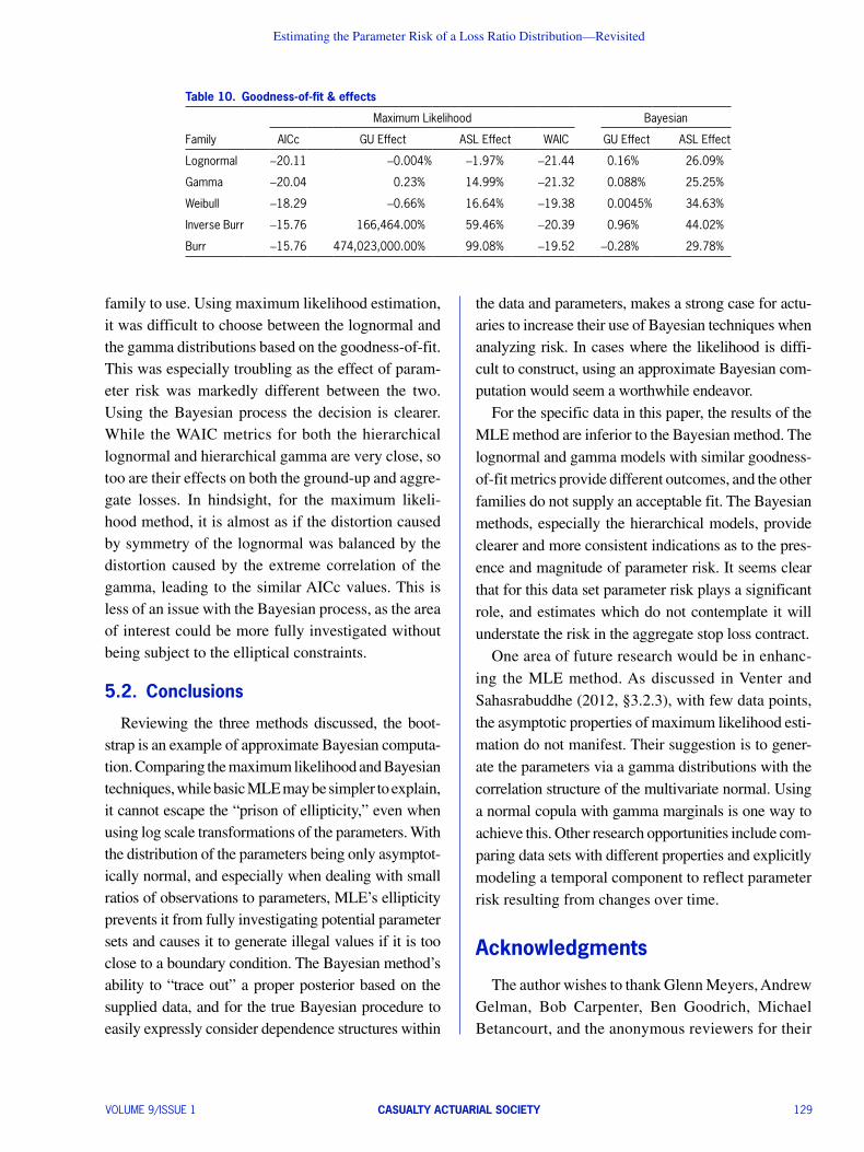
For the specific data in this paper, the results of the MLE method are inferior to the Bayesian method. The lognormal and gamma models with similar goodness-of-fit metrics provide different outcomes, and the other families do not supply an acceptable fit. The Bayesian methods, especially the hierarchical models, provide clearer and more consistent indications as to the pres-ence and magnitude of parameter risk. It seems clear that for this data set parameter risk plays a significant role, and estimates which do not contemplate it will understate the risk in the aggregate stop loss contract.

One area of future research would be in enhanc-ing the MLE method. As discussed in Venter and Sahasrabuddhe (2012, §3.2.3), with few data points, the asymptotic properties of maximum likelihood esti-mation do not manifest. Their suggestion is to gener-ate the parameters via a gamma distributions with the correlation structure of the multivariate normal. Using a normal copula with gamma marginals is one way to achieve this. Other research opportunities include com-paring data sets with different properties and explicitly modeling a temporal component to reflect parameter risk resulting from changes over time.

Acknowledgments

The author wishes to thank Glenn Meyers, Andrew Gelman, Bob Carpenter, Ben Goodrich, Michael Betancourt, and the anonymous reviewers for their

family to use. Using maximum likelihood estimation, it was difficult to choose between the lognormal and the gamma distributions based on the goodness-of-fit. This was especially troubling as the effect of param-eter risk was markedly different between the two. Using the Bayesian process the decision is clearer. While the WAIC metrics for both the hierarchical lognormal and hierarchical gamma are very close, so too are their effects on both the ground-up and aggre-gate losses. In hindsight, for the maximum likeli-hood method, it is almost as if the distortion caused by symmetry of the lognormal was balanced by the distortion caused by the extreme correlation of the gamma, leading to the similar AICc values. This is less of an issue with the Bayesian process, as the area of interest could be more fully investigated without being subject to the elliptical constraints.

5.2. Conclusions

Reviewing the three methods discussed, the boot-strap is an example of approximate Bayesian computa-tion. Comparing the maximum likelihood and Bayesian techniques, while basic MLE may be simpler to explain, it cannot escape the “prison of ellipticity,” even when using log scale transformations of the parameters. With the distribution of the parameters being only asymptot-ically normal, and especially when dealing with small ratios of observations to parameters, MLE’s ellipticity prevents it from fully investigating potential parameter sets and causes it to generate illegal values if it is too close to a boundary condition. The Bayesian method’s ability to “trace out” a proper posterior based on the supplied data, and for the true Bayesian procedure to easily expressly consider dependence structures within

Table 10. Goodness-of-fit & effects

Maximum Likelihood Bayesian

Family AICc GU Effect ASL Effect WAIC GU Effect ASL Effect

Lognormal -20.11 -0.004% -1.97% -21.44 0.16% 26.09%

Gamma -20.04 0.23% 14.99% -21.32 0.088% 25.25%

Weibull -18.29 -0.66% 16.64% -19.38 0.0045% 34.63%

Inverse Burr -15.76 166,464.00% 59.46% -20.39 0.96% 44.02%

Burr -15.76 474,023,000.00% 99.08% -19.52 -0.28% 29.78%



Johnson, S. G., The NLopt Nonlinear-Optimization Package, 2010, http://ab-initio.mit.edu/nlopt.

Klugman, S. A., H. H. Panjer, and G. E. Willmot, Loss Models: From Data to Decisions, New York: Wiley, 1998.

Kruschke, J. K., Doing Bayesian Data Analysis: A Tutorial with R, JAGS, and Stan, 2nd ed., Boston: Academic Press, 2015.

Melnick, E. L., and A. Tenenbein, “Misspecifications of the Normal Distribution,” American Statistician 360 (4), 1982, pp. 372–373, http://amstat.tandfonline.com/doi/abs/10.1080/00031305.1982.10483052.

Plummer, M., “JAGS: A Program forAnalysis of Bayesian Graphical Models Using Gibbs Sampling,” in K. Hornik, F. Leisch, and A. Zeileis, eds., Proceedings of the Third Inter-national Workshop on Distributed Statistical Computing (DSC 2003), 2003, http://www.ci.tuwien.ac.at/Conferences/DSC-2003/Proceedings/Plummer.pdf.

R Core Team. R: A Language and Environment for Statistical Computing, R Foundation for Statistical Computing, Vienna, Austria, 2014, http://www.R-project.org/.

Rubin, D. B., “Bayesianly Justifiable and Relevant Frequency Calculations for the Applies Statistician,” Annals of Statistics 120 (4), 1984, pp. 1151–1172, http://projecteuclid.org/euclid.aos/1176346785.

Spiegelhalter, D. J., N. G. Best, B. P. Carlin, and A. Van Der Linde, “Bayesian Measures of Model Complexity and Fit,” Journal of the Royal Statistical Society: Series B (Statistical Methodology) 640 (4), 2002, pp. 583–639.

Stan Development Team, Stan: A C++ Library for Probability and Sampling, Version 2.5, 2014a, http://mc-stan.org/.

Stan Development Team, Stan Modeling Language Users Guide and Reference Manual, Version 2.5, October 2014b, http://mc-stan.org/.

Turner, B. M., and T. Van Zandt, “Hierarchical Approximate Bayesian Computation,” Psychometrika 790 (2), 2014, pp. 185–209, http://www.ncbi.nlm.nih.gov/pmc/articles/PMC4140414/.

Van Kampen, C. E., “Estimating the Parameter Risk of a Loss Ratio Distribution,” Casualty Actuarial Society Forum, Spring 2003, pp. 177–213 http://www.casact.org/research/dare/index. cfm?fa=view abstrID=5289.

Venter, G. G., and R. V. Sahasrabuddhe, “A Note on Parameter Risk,” Casualty Actuarial Society E-Forum, Summer (2) 2012, pp. 1–16, http://www.casact.org/research/dare/index.cfm?fa= view abstrID=6879.

Watanabe, S., “A Widely Applicable Bayesian Information Criterion,” Journal of Machine Learning Research 140 (1), 2013, pp. 867–897, http://jmlr.org/papers/v14/watanabe13a.html.

Wickham, H., Ggplot2: Elegant Graphics for Data Analysis, New York: Springer, 2009.

Xie, Y., Dynamic Documents with R and knitr, Boca Raton, FL: Chapman and Hall/CRC, 2013.

Ypma, J., Nloptr: R Interface to NLopt, 2014, http://cran.r-project.org/web/packages/nloptr/index.html, R package version 1.0.4.

helpful comments and suggestions. Any errors in the paper are solely the author’s own.

ReferencesActuarial Standards Board. Risk Evaluation in Enterprise Risk

Management. Technical Report 46, Actuarial Standards Board, 2012, http://www.actuarialstandardsboard.org/pdf/asop046_ 165.pdf.

Anscombe, F. J., “Graphs in Statistical Analysis,” The American Statistician 270 (1), 1973, pp. 17–21, http://www.jstor.org/stable/2682899.

Bååth, R., “Tiny Data, Approximate Bayesian Computation and the Socks of Karl Broman,” Publishable Stuff: Rasmus Bååth’s Research Blog, October 2014. http://www.sumsar.net/ blog/2014/10/tiny-data-and-the-socks-of-karl-broman/ [Accessed 2015-01-22].

Beaumont, M. A., W. Zhang, and D. J. Balding, “Approximate Bayesian Computation in Population Genetics,” Genetics 1620 (4), 2002, pp. 2025–2035, http://www.genetics.org/ content/162/4/2025.abstract.

Bornn, L., N. Pillai, A. Smith, and D. Woodard, “One Pseudo- Sample is Enough in Approximate Bayesian Computa-tion MCMC,” ArXiv e-prints, 2014, http://arxiv.org/abs/ 1404.6298v3.

Burnham, K. P., and D. R. Anderson, Model Selection and Multi-model Inference: A Practical Information-Theoretic Approach, 2nd ed., New York: Springer Science+Business Media, 2002.

Denwood, M. J., “Runjags: An R Package Providing Interface Utilities, Model Templates, Parallel Computing Methods and Additional Distributions for MCMC Models in JAGS,” Jour-nal of Statistical Software, in press, http://runjags.sourceforge.net. R package version 1.2.1-0.

Eddelbuettel, D., and R. François, “Rcpp: Seamless R and C++ Integration,” Journal of Statistical Software 400 (8), 2011, pp. 1–18, http://www.jstatsoft.org/v40/i08/.

Geary, R. C., “The Distribution of ‘Student’s’ Ratio for Non-Normal Samples,” Supplement to the Journal of the Royal Statistical Society 30 (2), 1936, pp. 178–184, http://www.jstor.org/stable/2983669.

Gelman, A., J. B. Carlin, H. S. Stern, D. B. Dunson, A. Vehtari, and D. B. Rubin, Bayesian Data Analysis, 3rd ed., Boca Raton, FL: CRC, 2014.

Genz, A., F. Bretz, T. Miwa, X. Mi, F. Leisch, F. Scheipl, and T. Hothorn, Mvtnorm: Multivariate Normal and t Distribu-tions, 2014, http://CRAN.R-project.org/package=mvtnorm. R package version 1.0-2.

Hoffman, M. D., and A. Gelman, “The No-U-Turn Sampler: Adaptively Setting Path Lengths in Hamiltonian Monte Carlo,” Journal of Machine Learning Research 15, 2014, pp. 1593–1623, http://jmlr.org/papers/v15/hoffman14a.html.



there is a fundamental difference, such as a different kind of graph or a different structure for the negative log-likelihood function, the individual code chunks will be shown.

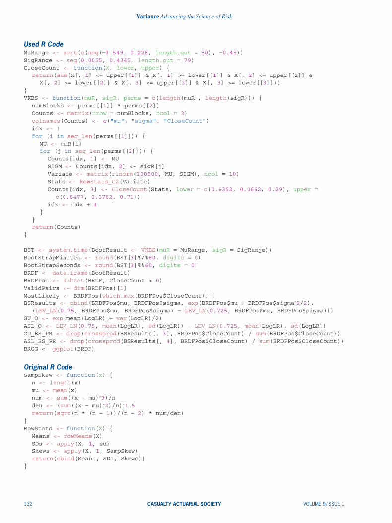
tic calculations. These were rewritten in C++ using the Rcpp package (Eddelbuettel and François 2011), bringing the elapsed time to under two minutes! Rcpp does require that the user is able to compile C++ code; in the Windows environment, this usually requires Rtools. In the following sections, the R code actually used will be brought first, followed by the original ‘R’ code for the two time-consuming functions, followed by the substitute Rcpp-based C++ code used instead.

Appendix A. Code

There are a number of cases where code was reused, differing only in the distribution being analyzed. In these cases, only one example will be brought. Where

A.1.2. Bootstrap algorithm and analysisOriginally, the bootstrap code was written com-

pletely in R and took 36 minutes on an Intel i7-3740QM at 2.7Ghz running Windows 7 64bit with 8GB RAM. This is orders of magnitude faster than the VBA code of the original paper, which took about 8 hours. However, the R implementation itself was sped up by profiling the code and identifying which elements were taking the most time—the sample skew and overall row statis-

A.1. Bootstrap-related code

A.1.1. Set-upset.seed(63854)library(ggplot2)library(reshape2)library(Rcpp)library(nloptr)library(mvtnorm)library(scatterplot3d)

LogLR <- c(-0.5376, -0.4388, -0.3953, -0.6415, -0.5376, -0.4388, -0.244, -0.3488, -0.4786, -0.4388)

LR <- exp(LogLR)ASL <- pmin(pmax(LR - 0.725, 0), 0.025)BayesData <- list(LR = LR, N = length(LR))

sourceCpp("BootC4.cpp")

AICC <- function(NLL, k, n) { k2 <- k * 2 return(2 * NLL + k2 + k2 * (k + 1)/(n - k - 1))}

WAIC <- function(pointMatrix) { colVars <- function(Matrix) { vars <- Matrix[1, ] for (n in seq_along(vars)) vars[n] <- var(Matrix[, n]) return(vars) } lppd <- sum(log(colMeans(pointMatrix))) pWAIC2 <- sum(colVars(log(pointMatrix))) return(-2 * (lppd - pWAIC2))}



Used R CodeMuRange <- sort(c(seq(-1.549, 0.226, length.out = 50), -0.45))SigRange <- seq(0.0055, 0.4345, length.out = 79)CloseCount <- function(X, lower, upper) { return(sum(X[, 1] <= upper[[1]] & X[, 1] >= lower[[1]] & X[, 2] <= upper[[2]] &

X[, 2] >= lower[[2]] & X[, 3] <= upper[[3]] & X[, 3] >= lower[[3]]))}VKBS <- function(muR, sigR, perms = c(length(muR), length(sigR))) { numBlocks <- perms[[1]] * perms[[2]] Counts <- matrix(nrow = numBlocks, ncol = 3) colnames(Counts) <- c("mu", "sigma", "CloseCount") idx <- 1 for (i in seq_len(perms[[1]])) { MU <- muR[i] for (j in seq_len(perms[[2]])) { Counts[idx, 1] <- MU SIGM <- Counts[idx, 2] <- sigR[j] Variate <- matrix(rlnorm(100000, MU, SIGM), ncol = 10) Stats <- RowStats_C2(Variate) Counts[idx, 3] <- CloseCount(Stats, lower = c(0.6352, 0.0662, 0.29), upper =

c(0.6477, 0.0762, 0.71)) idx <- idx + 1 } } return(Counts)}

BST <- system.time(BootResult <- VKBS(muR = MuRange, sigR = SigRange))BootStrapMinutes <- round(BST[3]%/%60, digits = 0)BootStrapSeconds <- round(BST[3]%%60, digits = 0)BRDF <- data.frame(BootResult)BRDFPos <- subset(BRDF, CloseCount > 0)ValidPairs <- dim(BRDFPos)[1]MostLikely <- BRDFPos[which.max(BRDFPos$CloseCount), ]BSResults <- cbind(BRDFPos$mu, BRDFPos$sigma, exp(BRDFPos$mu + BRDFPos$sigma∧2/2),

(LEV_LN(0.75, BRDFPos$mu, BRDFPos$sigma) - LEV_LN(0.725, BRDFPos$mu, BRDFPos$sigma)))GU_O <- exp(mean(LogLR) + var(LogLR)/2)ASL_O <- LEV_LN(0.75, mean(LogLR), sd(LogLR)) - LEV_LN(0.725, mean(LogLR), sd(LogLR))GU_BS_PR <- drop(crossprod(BSResults[, 3], BRDFPos$CloseCount) / sum(BRDFPos$CloseCount))ASL_BS_PR <- drop(crossprod(BSResults[, 4], BRDFPos$CloseCount) / sum(BRDFPos$CloseCount))BRGG <- ggplot(BRDF)

Original R CodeSampSkew <- function(x) { n <- length(x) mu <- mean(x) num <- sum((x - mu)∧3)/n den <- (sum((x - mu)∧2)/n)∧1.5 return(sqrt(n * (n - 1))/(n - 2) * num/den)}RowStats <- function(X) { Means <- rowMeans(X) SDs <- apply(X, 1, sd) Skews <- apply(X, 1, SampSkew) return(cbind(Means, SDs, Skews))}



Replacement C11 Code# include <Rcpp .h># include <math .h>using namespace Rcpp ;

// [[ Rcpp :: export ]]double SampSkew_C ( NumericVector X) { int n = X. size (); double Mu = mean (X); NumericVector XM = X - Mu; NumericVector D1 = XM * XM; NumericVector N1 = D1 * XM; double N2 = sum (N1) / n; double D1a = sum (D1) / n; double D2 = sqrt (D1a * D1a * D1a ); double P = sqrt (n * (n - 1)) / (n - 2); return P * N2 / D2;}

// [[ Rcpp :: export ]]NumericMatrix RowStats_C2 ( NumericMatrix X) { int nrow = X. nrow (); int ncol = X. ncol (); double n1 = ncol - 1.0; double P = ncol * sqrt (n1) / ( ncol - 2.0); NumericMatrix Results (nrow , 3); for (int i = 0; i < nrow ; ++i) { double M1 = 0.0; double M2 = 0.0; double M3 = 0.0; for (int j = 0; j < ncol ; ++j) { double delta = X(i, j) - M1; double delta_j = delta / (j + 1); double T1 = delta * delta_j * j; M1 + = delta_j ; M3 + = (T1 * delta_j * (j - 1) - 3 * delta_j * M2 ); M2 + = T1; } Results (i, 0) = M1; Results (i, 1) = sqrt (M2 / n1 ); Results (i, 2) = P * M3 / sqrt (M2 * M2 * M2 ); } return Results ;}

A.1.3. Bootstrap graphsContour graphBRGG + stat_contour(aes(x = sigma, y = mu, z = CloseCount, fill = . . level. .),

geom = "polygon") + scale_fill_gradient(low = "red", high = "yellow") + coord_cartesian(xlim = c(0.05, 0.25), ylim = c(-0.85, -0.05)) + scale_y_continuous(expression(mu)) + scale_x_continuous(expression(sigma))

A.2. Maximum likelihood related formulæ

A.2.1. First example likelihood surfacex <- y <- seq(1, 2, 0.1)f1 <- function(x, y) { 4 * (x - 1.5)∧2 + 4 * (y - 1.5)∧2}



f2 <- function(x, y) { 0.5 * (x - 1.5)∧2 + 0.5 * (y - 1.5)∧2}zf1 <- outer(x, y, f1)zf2 <- outer(x, y, f2)persp(x, y, zf1, theta = 45, phi = 30, shade = 0.1, col = "orangered", xlim = c(1, 2),

ylim = c(1, 2), zlim = c(0, 1.5), zlab = "Likelihood")

A.2.2. Maximum likelihood functionsLognormal

Two parameter representative example:

NLL_LN <- function(pars, X) { m <- pars[[1]] s <- pars[[2]] return(-sum(-log(X) - log(s) - 0.5 * log(2 * pi) - 0.5 * ((log(X) - m)/s)∧2))}GH_LN <- deriv3(~-(-log(X) - log(s) - 0.5 * log(2 * pi) - 0.5 * ((log(X) - m)/s)∧2),

c("m", "s"), function(m, s, X) NULL)NLLG_LN <- function(pars, X) { m <- pars[[1]] s <- pars[[2]] colSums(attr(GH_LN(m, s, X), "gradient"))}NLLH_LN <- function(pars, X) { m <- pars[[1]] s <- pars[[2]] colSums(attr(GH_LN(m, s, X), "hessian"))}ULEV_LN <- function(mu, sigma) { return(exp(mu + sigma∧2/2))}LEV_LN <- function(x, mu, sigma) { Z1 <- (log(x) - mu - sigma∧2)/sigma Z2 <- (log(x) - mu)/sigma return(ULEV_LN(mu, sigma) * pnorm(Z1) + x * pnorm(Z2, lower.tail = FALSE))}

Inverse Burr Three parameter representative example:

NLL_IB <- function(pars, X) { t <- pars[[1]] g <- pars[[2]] q <- pars[[3]] return(-sum(log(t) + log(g) + g * t * log(X/q) - log(X) - (t + 1) * log1p((X/q)∧g)))}GH_IB <- deriv3(~-(log(t) + log(g) + g * t * log(X/q) - log(X) - (t + 1) *

log((1 + (X/q)∧g))), c("t", "g", "q"), function(t, g, q, X) NULL)NLLG_IB <- function(pars, X) { t <- pars[[1]] g <- pars[[2]] q <- pars[[3]] colSums(attr(GH_IB(t, g, q, X), "gradient"))}NLLH_IB <- function(pars, X) { t <- pars[[1]] g <- pars[[2]] q <- pars[[3]] colSums(attr(GH_IB(t, g, q, X), "hessian"))



}ULEV_IB <- function(t, g, q) { return(exp(log(q) + lgamma(t + 1/g) + lgamma(1 - 1/g) - lgamma(t)))}LEV_IB <- function(X, t, g, q) { u <- ((X/q)∧g)/(1 + ((X/q)∧g)) First <- pbeta(u, t + 1/g, 1 - 1/g) Second <- 1 - u∧t return(ULEV_IB(t, g, q) * First + X * Second)}GenIB <- function(quantile, t, g, q) { P1 <- quantile∧(1/t) return(((P1/(1 - P1))∧(1/g)) * q)}

A.2.3. Maximum likelihood evaluationLognormal

Two parameter representative example:MLEfit_LN <- nloptr(c(1, 1), eval_f = NLL_LN, eval_grad_f = NLLG_LN, X = LR, lb = c(-Inf, 0), ub = c(Inf, Inf), opts = list(algorithm = "NLOPT_LD_LBFGS", maxeval = 10000,

xtol_rel = 1e-12, ftol_rel = 1e-12))VCoV_LN <- chol2inv(chol(NLLH_LN(MLEfit_LN$solution, LR)))SDs_LN <- sqrt(diag(VCoV_LN))ParCor_LN <- cov2cor(VCoV_LN)AICC_LN <- AICC(MLEfit_LN$objective, 2, length(LR))

Inverse Burr Three parameter representative example:

MLEfit_IB <- nloptr(c(1, 5, 2), eval_f = NLL_IB, eval_grad_f = NLLG_IB, X = LR, lb = c(0, 0, 0), ub = c(Inf, Inf, Inf), opts = list(algorithm = "NLOPT_LD_LBFGS", maxeval = 10000, xtol_rel = 1e-12, ftol_rel = 1e-12))

VCoV_IB <- chol2inv(chol(NLLH_IB(MLEfit_IB$solution, LR)))SDs_IB <- sqrt(diag(VCoV_IB))ParCor_IB <- cov2cor(VCoV_IB)AICC_IB <- AICC(MLEfit_IB$objective, 3, length(LR))

A.2.4. Stochastic simulation with MLE-based parameter riskMLE_PR_Simulate <- function(n, pars, sigma) { Simulation <- matrix(nrow = n, ncol = length(pars)) Simulation <- rmvnorm(n, mean = pars, sigma = sigma) return(Simulation)}

Lognormal simulation Two parameter representative example:

MLESimulation_LN <- MLE_PR_Simulate(n = 1000000, pars = MLEfit_LN$solution, sigma = VCoV_LN)LN_GU_Sim <- rlnorm(length(MLESimulation_LN[, 1]), meanlog = MLESimulation_LN[, 1],

sdlog = MLESimulation_LN[, 2])LN_AGG_Sim <- pmin(0.025, pmax(LN_GU_Sim - 0.725, 0))GU_MLE_PR_LN <- mean(LN_GU_Sim, na.rm = TRUE, trim = 0.001)ASL_MLE_PR_LN <- mean(LN_AGG_Sim, na.rm = TRUE, trim = 0.001)MLE_LN_DF <- data.frame(MLESimulation_LN)names(MLE_LN_DF) <- c("mu", "sigma")



Inverse Burr simulation Three parameter representative example:

MLESimulation_IB <- MLE_PR_Simulate(n = 1000000, pars = MLEfit_IB$solution, sigma = VCoV_IB)IB_GU_Sim_Raw <- runif(1000000, 0, 1)IB_GU_Sim <- GenIB(IB_GU_Sim_Raw, MLESimulation_IB[, 1], MLESimulation_IB[, 2],

MLESimulation_IB[, 3])IB_AGG_Sim <- pmin(0.025, pmax(IB_GU_Sim - 0.725, 0))GU_MLE_PR_IB <- mean(IB_GU_Sim, na.rm = TRUE, trim = 0.001)ASL_MLE_PR_IB <- mean(IB_AGG_Sim, na.rm = TRUE, trim = 0.001)

A.2.5. MLE graphsMLE Lognormal ContourMLE_LN_G <- ggplot(MLE_LN_DF)MLE_LN_G + stat_density2d(aes(x = sigma, y = mu, fill = . .level. .), geom = "polygon")

+ scale_fill_gradient(low = "red", high = "yellow") + scale_y_continuous(expression(mu)) + scale_x_continuous(expression(sigma)) + stat_density2d(aes(x = sigma, y = mu), colour = "black")

A.3. Bayesian Analysis

A.3.1. JAGSSimple Lognormal Modelvar N, LR[N], mu.post, sigma.post, tau.post, LR.post, ASL.post, PointPosteriors [N];model { for (year in 1:N) { LR[ year ] ~ dlnorm (mu.post, tau.post) } mu.post ~ dnorm (0, 0.25) sigma.post ~ dunif (0, 1) tau.post <- pow( sigma.post, -2) LR.post ~ dlnorm (mu.post, tau.post) ASL.post <- min (0.025, max(LR. post - .725 , 0)) for (i in 1:N) { PointPosteriors [i] <- dlnorm (LR[i], mu.post, tau.post) }}

Simple Lognormal AnalysisinitsLN <- function(chain) { list(mu.post = rnorm(1, 0, 2), sigma.post = runif(1, 0, 1), .RNG.seed = chain∧2 + 1,

.RNG.name = "base::Mersenne-Twister")}LN_Model <- run.jags(model = "Bayes_LN.bug", monitor = c("mu.post", "sigma.post",

"LR.post", "ASL.post", "PointPosteriors"), data = BayesData, n.chains = 5, plots = TRUE, psrf.target = 1.01, check.stochastic = TRUE, modules = c("bugs", "glm"), method = "interruptible", adapt = 25000, burnin = 25000, sample = 10000, thin = 25, inits = initsLN)

Comb_LN <- combine.mcmc(LN_Model)BayesGU_LN <- LN_Model$summary$statistics[2, 1]BayesASL_LN <- LN_Model$summary$statistics[1, 1]BayesWAIC_LN <- WAIC(Comb_LN[, 4:13])BayesParCor_LN <- LN_Model$crosscorr[3, 14]BayesDF_LN <- data.frame(Comb_LN[, 3], Comb_LN[, 14])names(BayesDF_LN) <- c("mu", "sigma")



A.3.2. StanSimple Lognormal Modeldata { int < lower = 0> N; // number of years vector < lower = 0.0 >[N] LR; // loss ratios}parameters { real mu; // prior for mu real < lower = 0.0 > sigma ; // non - negative prior for sigma}model { mu ~ normal (0.0 , 2.0); sigma ~ uniform (0.0 , 1.0); LR ~ lognormal (mu , sigma );}generated quantities { real LR_post ; // distribution of LR based on posterior parameters real ASL_post ; // corresponding ASL vector [N] PointPosteriors ; // log pointwise predictive density for (i in 1:N) { PointPosteriors [i] <- exp( lognormal_log (LR[i], mu , sigma )); } LR_post <- lognormal_rng (mu , sigma ); // stochastic observation of LR ASL_post <- fmin (0.025 , fmax ( LR_post - 0.725 , 0.0));}

Hierarchical Lognormal Modeldata { int < lower = 0> N; // number of years vector < lower = 0.0 >[N] LR; // loss ratios}parameters { vector [2] mu; // multivariate normal (MVN ) prior mean : implied (0 ,0) corr_matrix [2] Sigma_corr ; // MVN prior correlation ( implied uniform ) vector < lower = 0.0 >[2] Sigma_scale ; // prior scale for cov: implied (0 ,0) vector [2] Pars ; // correlated lognormal parameter vector}transformed parameters { real mu_post ; real < lower = 0.0 > sigma_post ; mu_post <- Pars [1]; sigma_post <- exp( Pars [2]); // ensure non - negativity}model { matrix [2, 2] Sigma ; // will become MVN prior covariance Sigma <- diag_matrix ( Sigma_scale ) * cholesky_decompose ( Sigma_corr ); Pars ~ multi_normal_cholesky (mu , Sigma ); // faster to use cholesky LR ~ lognormal ( mu_post , sigma_post );}generated quantities { real LR_post ; // distribution of LR based on posterior parameters real ASL_post ; // corresponding ASL vector [N] PointPosteriors ; // log pointwise predictive density for (i in 1:N) { PointPosteriors [i] <- exp( lognormal_log (LR[i], mu_post , sigma_post )); } LR_post <- lognormal_rng ( mu_post , sigma_post ); // stochastic observation of LR ASL_post <- fmin (0.025 , fmax ( LR_post - 0.725 , 0.0));}



Lognormal AnalysisLNP_S <- stan(file = "Bayes_LN_Plus2.stan", data = BayesData, pars = c("mu_post",

"sigma_post", "LR_post", "ASL_post", "PointPosteriors"), iter = 20200, warmup = 200, thin = 1, chains = 5, seed = 82, refresh = -1, verbose = FALSE)

LNP_S_E <- extract(LNP_S)StanGU_LNP <- mean(LNP_S_E$LR_post)38StanASL_LNP <- mean(LNP_S_E$ASL_post)StanWAIC_LNP <- WAIC(LNP_S_E$PointPosteriors)StanDF_LNP <- data.frame(LNP_S_E$mu_post, LNP_S_E$sigma_post)names(StanDF_LNP) <- c("mu", "sigma")StanCor_LNP <- cor(StanDF_LNP)["mu", "sigma"]

Inverse Burr Model Example of manually creating distribution functions

data { int < lower = 0> N; // number of years vector < lower = 0.0 >[N] LR; // loss ratio}parameters { real < lower = 0.0 > tau ; real < lower = 0.0 > gamma ; real < lower = 0.0 > theta ;}transformed parameters { vector < lower = 0.0 >[N] U; U <- LR / theta ;}model { tau ~ uniform (0.0 , 100.0); gamma ~ uniform (0.0 , 100.0); theta ~ uniform (0.0 , 1.0); for (i in 1:N) { increment_log_prob (log( gamma * tau) + multiply_log (( gamma * tau), U[i]) - fma

(( tau + 1), log1p (pow (U[i], gamma )), log (LR[i ]))); }}generated quantities { real LR_post ; real ASL_post ; real < lower = 0.0 , upper = 1.0 > Q; // quantile for inversion real < lower = 0.0 > P1; // Reused value vector [N] PointPosteriors ; for (i in 1:N) { PointPosteriors [i] <- exp(log(tau) + log( gamma ) + multiply_log (( gamma * tau ),

U[i]) - fma (( tau + 1), log1p (pow(U[i], gamma )), log(LR[i ]))); } P1 <- pow( uniform_rng (0.0 , 1.0) , inv (tau )); // using inversion LR_post <- pow (( P1 / (1 - P1 )), inv ( gamma )) * theta ; ASL_post <- fmin (0.025 , fmax ( LR_post - 0.725 , 0.0));}

A.4. Conclusion and findings

A.4.1. Superimposed contour plotBRGG + stat_contour(aes(x = sigma, y = mu, z = CloseCount, colour = "Bootstrap"),

alpha = 0.4, size = 1) + scale_y_continuous(expression(mu)) + scale_x_continuous (expression(sigma)) + stat_density2d(aes(x = sigma, y = mu, colour = "MLE"), alpha = 0.4, size = 1, data = MLE_LN_DF) + stat_density2d(aes(x = sigma, y = mu, colour =



"Bayes (Simple)"), alpha = 0.6, size = 1, data = StanDF_LN) + theme(legend.title = element_blank())

A.4.2. Inverse Burr scatter plot (MLE)scatterplot3d(MLESimulation_IB, pch = ".", xlab = expression(tau), ylab = expression(gamma),

zlab = expression(theta), highlight.3d = FALSE, cex.lab = 2, xlim = c(-10, 100), ylim = c(-20, 100), zlim = c(0, 1))

A.4.3. Color-coded inverse Burr scatter plot (Bayesian)scatterplot3d(StanDF_IB, pch = ".", xlab = expression(tau), ylab = expression(gamma),

zlab = expression(theta), highlight.3d = FALSE, cex.lab = 2, xlim = c(-10, 100), ylim = c(-20, 100), zlim = c(0, 1), color = GUColorPalette_S_IB, angle = 5)

A.5. Session info## R version 3.2.3 Patched (2015-12-13 r69768)## Platform: x86_64-w64-mingw32/x64 (64-bit)## Running under: Windows 7 x64 (build 7601) Service Pack 1#### locale:## [1] LC_COLLATE=English_United States.1252## [2] LC_CTYPE=English_United States.1252## [3] LC_MONETARY=English_United States.1252## [4] LC_NUMERIC=C## [5] LC_TIME=English_United States.1252#### attached base packages:## [1] stats graphics grDevices utils datasets methods base40#### other attached packages:## [1] rstan_2.8.2 inline_0.3.14 runjags_2.0.3-1## [4] rjags_4-4 coda_0.18-1 lattice_0.20-33## [7] scatterplot3d_0.3-36 mvtnorm_1.0-3 nloptr_1.0.4## [10] Rcpp_0.12.2 reshape2_1.4.1 ggplot2_2.0.0## [13] knitr_1.11#### loaded via a namespace (and not attached):## [1] magrittr_1.5 munsell_0.4.2 colorspace_1.2-6 highr_0.5.1## [5] stringr_1.0.0 plyr_1.8.3 tools_3.2.3 parallel_3.2.3## [9] grid_3.2.3 gtable_0.1.2 digest_0.6.8 gridExtra_2.0.0## [13] formatR_1.2.1 codetools_0.2-14 evaluate_0.8 stringi_1.0-1## [17] scales_0.3.0 stats4_3.2.3