Embed Size (px)
Citation preview
Estimating the Output Gap:
A Kalman filter approach1
Draft version, please do not quote.
30 June 2004
Özer Karagedikli and L. Christopher Plantier
The output gap plays a crucial role in the thinking of many inflation targeting central banks. At the same time, real time estimates of the output gap undergo substantial revisions as more data become available. In this paper, we employ a state space framework to augment the simple Hodrick-Prescott filter with additional structural equations to i) reduce the size of revisions and ii) reduce the uncertainty around the mean real time output gap estimates. In particular we use the relationship between output and the capacity utilisation and output and unemployment to infer the unobserved potential output. Our technique is demonstrated on data for New Zealand, but is applicable elsewhere as well.
JEL: C32, E32
Key Words: Output Gap, Kalman filter, New Zealand
1 Özer Karagedikli is with the Economics Department, Reserve Bank of New Zealand and Chris Plantier is with the International Affairs of the US Treasury. The views expressed here are the views of the authors and do not necessarily represent the views of their employers. We would like to thank Olivier Basdevant, Nils Björksten, Tim Hampton, Angela Huang, Satish Ranchhod and the seminar participants at the Reserve Bank of New Zealand and the University of Otago. Corresponding author Özer Karagedikli. Email: [email protected]
2
1 Introduction
The output gap is defined as deviations of actual output from potential output, where potential output is the level of output that is consistent with the productive capacity of the economy. Yet this ‘potential output’ concept is not observed. Like many other central banks, the Reserve Bank of New Zealand also relies on this ‘unobserved measure’ in its policy making. Black, Cassino, Drew, Hansen, Hunt, Rose and Scott (1997) show that in the Forecasting and the Policy System (FPS), the Reserve Bank of New Zealand’s main macroeconomic model, domestic inflation is determined within a Phillips curve framework using the output gap.
In this paper, we estimated an augmented Hodrick-Prescott filter, proposed by Laxton and Tetlow (1992) but with the Kalman filter. Because this approach encompasses the Reserve Bank of New Zealand’s multivariate filter, in this way, we are able to test the sensitivities of the estimates to different assumptions. We demonstrate that, there is a considerable uncertainty around the output gap estimates. In addition, we demonstrate that, different models, based on different assumptions, can be presented in a ‘thick modelling’ sense.
The remainder of the paper is structured as follows: Section 2 discusses the related literature. Section 3 discusses the HPMV filter in general ( a la Laxton and Tetlow, LT hereafter) and in state space. Section 4 discusses the advantages of the Kalman filter approach over the iterative LT approach. Section 5 presents the results of our approach under different assumptions and trend specifications. Section 6 briefly talks about the revision properties of the output gap estimates from our models. Section 7 concludes.
2 Literature review
It has been widely discussed that the central banks are not good predictors of the output gap in real time. What seems a perfectly good predictor of inflation ex-post, does not work in real time. Two very recent papers highlighted this: One by the Reserve Bank of Australia found that the real time output gaps, based on the Reserve Bank of Australia (Stone et al 2003) filters, are not good forecaster of inflation. Second is a more substantial piece on the US economy. In this paper Orphanides and van Norden (2003) look at the real time inflation predicting power of about 10 different output gap estimates, from Harvey (1985) to Kuttner (1994). The conclusion is almost identical that the relationship is very good ex-post, but not in real time. On the other hand, Graff (2004) states that the Reserve Bank of New Zealand’s output gap measure does predict the non-tradable inflation well, despite the other problems associated with the methodology.
Because the output gap concept is not observable, economists try to estimate it. As is the case in many other areas of economics, there are more than one ways of estimating the output gap, yet probably no one knows which estimate is the correct one, especially in real time. Hence, a different technique or model that comes with a different output gap profile should not be disregarded; it should be regarded as ‘one estimate’. This approach of considering many specifications, can be regarded as a ‘thick modelling’ exercise proposed by Granger and Jeon (2004).

3
It is quite a standard practice in economic modelling to distinguish the long-run properties of a system from its fluctuations around the long-run trend. There are various approaches to do this, but what is interesting is that most of these can be conveniently represented within a state-space model.
Apart from the mechanical filters such as the HP, ARMA and linear filters, unobserved components models provide an alternative framework for estimating the output gap. Unobserved components models decompose the observed output into its trend and cycle components. Watson (1986), Harvey (1985), Clark (1989) and Harvey and Jeager (1993) are examples of this approach. Kuttner (1994) adds a Phillips curve to the univariate model of Watson and Gerlach and Smets (1997) models modifies Harvey (1985) and Clark (1987) approached by adding a Phillips curve equation. Very recently, Benes, J and P N’Diaye (2004), estimated a so-called multivariate filter for the Chech Republic.
At the Reserve Bank of New Zealand, a lot of research has been undertaken with regard to the output gap. Scott (1997) estimated a common cycles model a la Clark (1989). Claus (2003) estimates a structural vector autoregression to estimate the output gap. The main model the RBNZ uses for the output gap estimation is a modified HP filter, a la Laxton and Tetlow (1992), so-called the multivariate (MV) filter. Conway and Hunt (1997) detail the approach and Hampton (2002) modifies it slightly. This type of modelling of the output gap is often referred as the, Hodrick-Prescott Multivariate, HPMV, filter.
In this paper, we will pursue this HPMV filter approach. HPMV approach in state space has been used in estimating unobserved variables, such as non-accelerating inflation rate of unemployment, NAIRU (OECD 2000) output gap or the neutral real interest rate previously (Basdevant et al 2004). There are two advantages of this approach: One, it is semi-structural, i.e. it includes a mechanical filter, as well as some economic structure. Second, because the HPMV is the way the Reserve Bank of New Zealand estimates the output gap, putting the HPMV in state-space and estimating it with different assumptions, may tell us the advantages and disadvantages of certain assumptions, and guide us towards a better way of estimating the output gap. This also enables us to test the sensitivity of the Bank’s MV filter to different assumptions. As Boone (2002) states two approaches are closely linked, and specifically. Estimating the HPMV filter by using the Kalman filter has at least two advantages. First, while the traditional HPMV filter cannot produce margins of uncertainty for the estimated variables, the Kalman filter can. Secondly, it allows wider evaluation of the impact of the different assumptions underlying each technique on the estimates of the unobserved variables.
3 The HPMV framework and the Kalman filter
LT argue that the simple Hodrick Prescott filter can be augmented with residuals coming from structural relationships. Hence mimimising this new set of problem would be better than a mechanical Hodrick-Prescott (HP hereafter) filter. Because the HPMV is a an augmented HP filter, or its starting point is an HP filter, let us start with the conventional Hodrick-Prescott filter and put it in state-space The HP filter gives an estimate of the unobserved variable as the solution to the following minimisation problem:
{ } ( ) ( )∑ =∆+−T
t ttty
yyyMint
1
*212*121
20* σσ (1)
4
Where y is the observed variable, y* is the unobserved variable being filtered, 20σ is the
variance of the cyclical component y−y* and 21σ is the variance of the growth rate of the
trend component. This problem is of course invariant to a homothetic transformation;
therefore what matters is the ratio 21
20
1 σσλ = . Hodrick and Prescott suggest some
parameterisation of λ1 depending on the frequency of data2. Following Harvey (1985), the HP filter can be written in a state space form as follows. The measurement equation defines the observed variable as the sum of its trend and fluctuations around the trend:
ttt eyy += * (2)
with ),0(~ 20σNet . The state equations define the growth rate of the trend that is
accumulated to compute the trend itself:
tttt ygy ,1*
11* ν++= −− (3)
ttt gg ,21 ν+= − (4)
with 0,1 =tv (no shock to the level of potential output) and tt vN ,2120,2 ),0(~ λσν
is the
change in the growth rate of the filtered series or trend. In other words, the change in the trend follows a random walk. Then to get the HP filter estimate one has to use the whole set of information to derive y* (as done in the minimisation problem (1)), ie to take the smoothed estimate provided by the Kalman filter.
The Hodrick Prescott Multi-Variate (HPMV hereafter) filter is an alternative way of estimating unobserved variables, developed at the Bank of Canada (see Laxton and Tetlow (1992))3. This method stems from use of the standard HP filter (see Hodrick and Prescott (1997)), augmented by relevant economic information. It has been used by the Central Banks of Canada and New Zealand to estimate potential output (see Butler (1996) and Conway and Hunt (1997)) and by OECD (1999) to estimate the NAIRU. Boone (2000) extends on Harvey (1985) and puts the HPMV filter in state space. This is done in two steps. Firstly, the minimisation problem is written as a state space model. Secondly, restrictions are imposed on the variances of the equations of the state space model, to reproduce the balance between the elements of the minimisation programme.
The HPMV filter seeks to estimate the unobserved variable as the solution to the following minimisation problem:
{ } ( ) ( )∑ =+∆+−T
t tttty
yyyMint
1
22
2*21
2*
*ζλλ (5)
With λ1 and λ2 given. This is a basic HP filter, augmented with the residuals ζt taken from an estimated economic relationship:
tttt dXyz ζβ ++= * (6)
2 100 for annual data, 400 for semi-annual data and 1600 for quarterly data. 3 See St Amant and van Norden (1997) for a critique of the iterative Laxton and Tetlow approach.
5
where z is another explanatory variable can be explained by the unobserved variable y*
and X is a matrix of other exogenous variables. The residuals ζ are normal with a covariance matrix H2.
As for the simple HP filter, the smoothing constants λ1 and λ2 reflect the weights attached to different elements of the minimisation problem. The estimated unobserved variable is not only a simple moving average going through the observed series, but is also modelled to give a better fit to the economic relationship. The HPMV filter can also be reproduced by a Kalman filter, following a similar methodology. In essence the problem is simply to add the additional structural equation in the set of measurement equations:
+
+
=
t
ttt
t
t eX
dy
z
y
ζβ01 * (7)
with ( ) ( )HNe tt ,0~′ζ . The covariance matrix H is defined as:
=
220
20
0
0
λσσ
H (8)
The two state-equations are the same as for the standard HP filter (see equations (3) and (4)). The novelty is the term λ2, which gives a balance between the HP filter and the economic information embodied in the additional equation. A high value for λ2
corresponds to a better fit of the economic relationship, and an unobserved variable that can depart significantly from the observed variable.
There are two advantages to be gained from reproducing an HPMV filter with the Kalman filter. Firstly, the method is done of simultaneous nature (while the method proposed by LT is a multi-step procedure4), and also allows estimation of the hyper-parameters. Thus, although it is rarely done in practice, it is possible to freely estimate the parameters λ1 and λ2 instead of giving these essentially arbitrary values.
The type of HPMV filter we have estimates has the following form:5
{ } ( ) ( )∑ =++∆+−T
t ttttty
yyyMint
1
2,23
2,12
2*21
2*
*ζλζλλ (9)
With λ1 to λ3 given, the residuals ζi,t corresponds to two relations: an Okun's law and a link between capacity utilisation survey data and the potential output:
( ) ttttt yyuu ,1*
11 ζβ +−+= −− (10)
( ) ttttt yyuccu ,2*
11 ζγ +−+= −− (11)
4 See Hampton, Twaddle (2002) and so on for this iterative procedure. 5 We should indicate that this is a first cut, a good first cut we believe, which can be improved further
with more conditioning information.

6
where y is the output and y* the potential output, u is the unemployment rate and cu the capacity utilisation rate that are taken as differences from their equilibrium value.6 We do not use the Phillips Curve due to the problem of circularity, suggested in Graff (2004).
4 Problems with the Laxton and Tetlow method and the advantages of the Kalman filter approach
In this section, we will discuss the shortcomings of the LT approach and how Kalman filter is superior to the iterative LT approach and can address some of the shortcomings of the LT approach.
The equations 10 and 11 are added to get more information from the structural economic relationships, which hopefully would help us at the end of the sample. However, these equations have additional problems too. It is obvious that the residuals that come out of these equations would be sensitive i) to the parameters, and ii) to the equilibrium values in these structural equations, i.e. equilibrium capacity utilisation rate and unemployment rate. Furthermore, how those residuals are weighted in the minimisation, namely 2λ
and
3λ would also matter.
The classic argument in favour of these augmenting equations is that these two variables are not revised. This is not completely true. Although their level values are not revised by the statistician, the reason why cu7 is not revised is because we assume we know what the trend or the equilibrium value is. It has been shown that the ex-post errors of a gap concept such as output gap and unemployment gap do not largely come from the revisions to the data; they come from getting the trend wrong in real time. Hence, saying that “we know the trend in cu or u”, does not overcome our problems.
The RBNZ’s MV filter-determined trend unemployment rate was by means of an HP filter up until 2002 (see Hampton 2002). Although the unemployment rate is not revised by the statistician, the gap measured by means of an HP filter still has very large revisions ex-post. Figure 1 below shows the revisions to the HP filtered unemployment gap in New Zealand.8
***Figure 1 about here***
Hampton (2002) attempts to overcome this problem by augmenting the HP filter with data from skill shortage surveys. The skill shortage data is a weighted average of skilled and unskilled labour shortage data by the Quarterly Survey of Business Opinion. 9
ttttt skillskilluu φκ +−+= )( (12)
However, this augmentation does not solve the problem. Again, this equation requires an equilibrium assumption. Equilibrium skill shortage, assumed by the current MV filter is plotted against an HP filtered trend and the actual skill shortage series in figure 2 below:
6 See Appendix B for the state-space model of our approach. 7 Capacity utilisation being a survey measure may further complicate the problems. 8 The same problem of course exists for the capacity utilisation equilibrium value. The Real Business
Cycle school would probably argue that the equilibrium capacity utilisation would be time varying. 9 This is a survey data collected by the New Zealand Institute of Economic Research, NZIER.
7
***Figure 2 about here***
As we can see, the way we filter can make a difference to the “skill shortage gap”. In fact, one can argue that the equilibrium value is a series with regime changes: Early 1990s, where it was easy to find labour, mid to late 1990s, where it was relatively harder to get labour. And finally the last few years, given very low unemployment rate, it may be the case that the pool of applicants for any given job ad is now smaller, hence the survey will have a lower negative mean for a while. Of course the main question is whether employers have to live with this tighter labour market environment and hence adjust or they will reflect this on their prices. The latter would mean a change in the equilibrium skill shortage series.
The shortcoming of the LT approach is that, it tries to solve the end-point problem in one trend, by introducing another variable with an unobserved trend. In addition, the trend unemployment rate is exogenous in the minimisation problem of the HPMV filter. The Kalman filter approach can overcome this problem in the following way: If we allow the unemployment rate to be an unobserved variable within the whole system, where unemployment is an unobserved, but the trend unemployment rate is included in the Okun’s law relationship. This is how we will approach to the modelling.
Another assumption in the RBNZ’ MV filter is that the coefficients are imposed, not estimated. The state space approach also allows us to examine the implications of imposing the coefficients in the structural equations. We start with the capacity utilisation equation. Let us estimate a few capacity utilisation equations:
ttttt yycucu εγ +−+= )( * (13)
First we estimate this with the ordinary least squares. The parameter γ
is estimated. However, we should be aware that the OLS estimator of the parameter γ
would suffer
from the simultaneity bias, since tcu and )( *tt yy − are determined simultaneously in the
economy. In addition, there is a severe serial correlation problem.
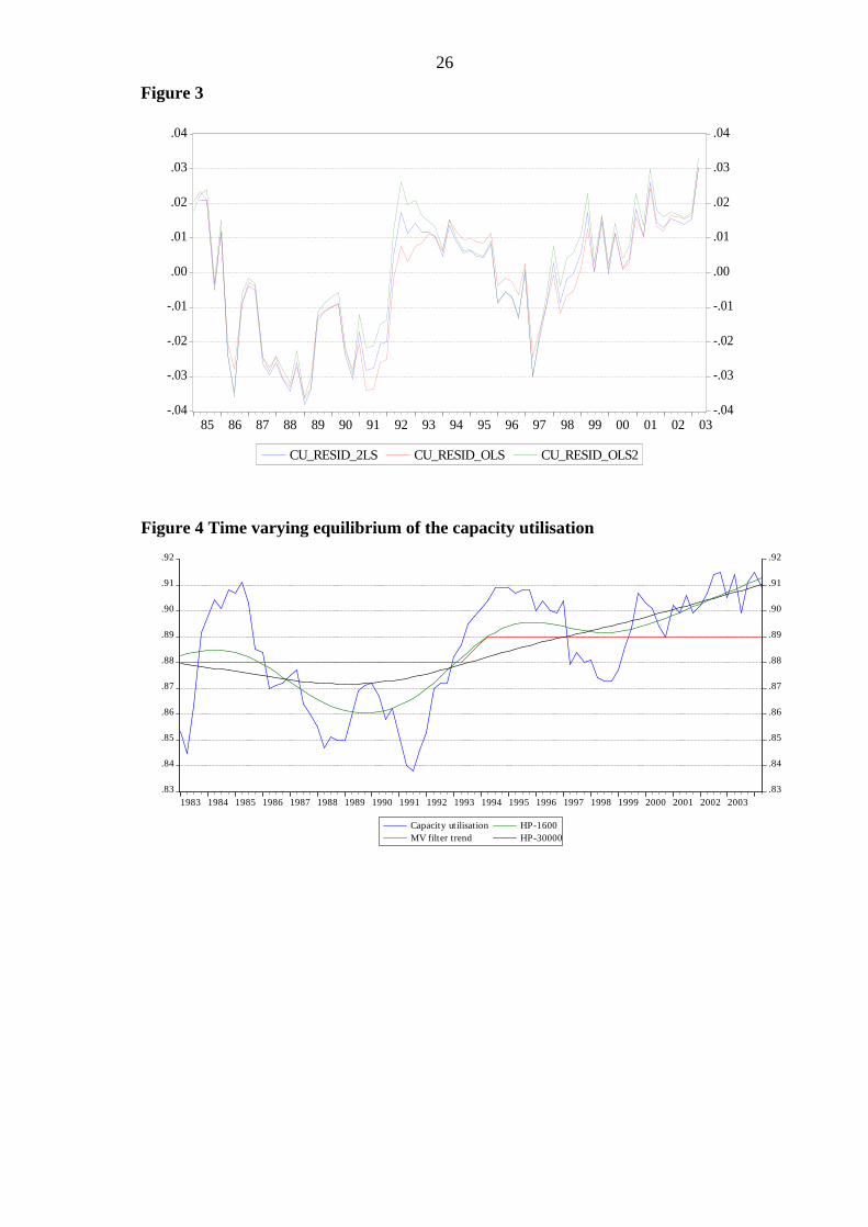
The first column of the Table 1 reports the results of the OLS regressions of the equation 12. The coefficient estimate is 0.629. The second column shows the two stage least square estimate by using the first lags of the capacity utilisation and the output gap. Figure 3 shows the residuals that would go into the minimisation problem of equation 9, under different estimates. It is clear that they are different at times and they may make difference to the final output gap estimates.
***Table 1 about here***
***Figure 3 about here***
Alternatively, one can allow the capacity utilisation equation to have a time varying equilibrium value and estimate it with the Kalman filter. We allowed for this with the following specification:
ttttt yycucu ,1*)( εγ +−+= (14)
cuttt gcucu 11 −− += 15)
8
tcut
cut gg ,21 ε+= − (16)
where, the first equation is the signal and the last two are the state equations. The choice of the signal to noise ratio of course does matter here. We chose a very stiff ratio of 30,000.
The estimated γ
is 0.56. Figure 4 below compares a few different equilibrium capacity utilisation rates: The RBNZ’s MV filter’s assumption, our simple state space model of equations 14-16 and two HP filtered trends with different smoothing parameters. It is clear that the trend can be so different. Hence the minimisation problem would be a different one, under a different trend assumption or estimation.
***Figure 4 about here***
Another major assumption in the original LT approach is that there is an explicit assumption on the trend output growth, called the ‘stiffener’. The stiffener explicitly assumes a trend growth rate for the end of the sample, hence disallows the filter to be very flexible in its view of the trend. This can be a dangerous approach to employ, as at times, the trend growth may be changing too fast before we realise it. This is another advantage of the Kalman filter approach is that there is no need for an explicit ‘stiffener’ in estimation procedure. Since most of the end point problem is more severe when the trend growth rate is changing fast, this assumption may increase the size of real time errors.
It is also important how the filter weights these additional information. If we think in terms of signal to noise ratio, these weights can make significant changes to the final estimates of the output gap. The Bank’s MV filter fixes these weights at some arbitrary numbers. The HPMV approach with the Kalman filter allows us to estimate these weights, given that we already impose one of the hyperparameters.
Original LT work suggests that it is difficult to estimate confidence intervals for their approach. However, despite its difficulties they come up with a confidence interval which is 4 per cent on either side of the mean estimate. This gives a range of 8 per cent. Because the state space approach enables us to estimate the potential output with standard errors, and because we know that the historical revisions to the level of GDP is very minor (which can be ignored), we can create confidence intervals for our output gap estimates. Below, we show the confidence intervals for our preferred model.
5 Estimating HPMV filters with the Kalman filter
Having discussed all the things that may matter for the final output gap estimates, we now present out HPMV filter in state space. We start with the following HPMV filter, which is the simplest form:
Signal equations
ttt yy ε+= * (17)
( ) ttttt yyuu ,1*
11 ζβ +−+= −− (18)

9
( ) tttt yyuccu ,2*
11 ζγ +−+= −− (19)
State equations
1*
1*
−− += ttt gyy (20)
ttt gg ε+= −1 (21)
where equations 17-19 are signal equations, and equations 20 and 21 are state equations.
We start with a baseline model, where our baseline model tries to replicate the Reserve Bank of New Zealand’s internal MV filter, as much as possible. We will then relax the assumptions of the MV filter as we discussed in the previous chapter.
The baseline model, Model 1 assumes an equilibrium capacity utilisation (time invariant) and equilibrium unemployment (time varying). These are determined outside the model we estimate here. Equilibrium capacity utilisation is 88 per cent until 1992 and then 99 per cent after 1992, which is exactly the same as what the Reserve Bank’s MV filter uses. This model also assumes that the equilibrium unemployment is an ex-post HP filtered unemployment rate and the equilibrium capacity utilisation is known with precision. In other words, there is no uncertainty with these two equilibrium values10. The advantage of this base model is that because it is very close to the current filtering approach used by the Reserve Bank, we can then relax some of the assumptions, or change things here and there to see if they make any difference and how much difference they make.
Table 2 below shows the estimation results from the basic HPMV filter. The trend unemployment rate is determined by an HP filter. Unemployment is filtered outside the system and then entered into the system here.
There are three variations of this base model. Model 1 imposes the coefficients on the Okun’s law and the capacity utilisation. The coefficient β
is the so-called Okun’s coefficient, which maps the changes in output gap to the changes in unemployment from its equilibrium. The coefficient suggests that for every 1 per cent deviation of output from its potential, the unemployment deviates from its natural rate by 0.33 per cent, which is a relationship of 1 to 3. This coefficient is very similar to the original estimates of Okun (1962) and slightly different that 1 to 2 relationship found by Scott (1997).
Coefficient γ
is the relationship between the capacity utilisation and the output gap. The calibrated coefficient of 1 means that a 1 per cent deviation of output from its trend leads the capacity utilisation to deviate 1 per cent from its trend.
***Table 2 about here***
The model 1 also imposes the trends in cu and u equations. The signal to noise ratios are also imposed at 1600, 2 and 2 respectively. These are all consistent with the Reserve Bank’s official filter.
10 This is also the case in the original Laxton and Tetlow (1992) approach, where the equilibrium unemployment rate was assumed to be known with no uncertainty around it.

10
Model 2, estimates the coefficients although still imposed the equilibrium values in capacity utilisation and unemployment. Hence the equilibrium unemployment is the same in these models. One major change in this model is the change in the coefficientγ . This implies that the relationship between capacity utilisation gap and the output gap may not be 1 to 1. The Wald test of 1=γ
is rejected at 5 per cent significance level. The
coefficient turns out 0.707. In other words, a 1 per cent output gap is associated with a capacity utilisation deviation of 0.7 per cent from its trend. The estimated Okun’s law coefficient is also different, -0.271. This indicated that a 1 per cent output gap implies unemployment to be differ by -0.271 per cent from its equilibrium.
In Model 3, in addition to estimating the coefficients, we also estimate the equilibrium capacity utilisation as a constant. This model makes further changes in coefficients. Estimated γ
is now closed to 1, 0.927. Furthermore, the Okun’s law coefficient is now much lower, indicating a weaker relation to the unemployment deviations from its trend from the output gap. The equilibrium capacity utilisation turns out to be 0.884 per cent,
which is very close to the Model 1, where cu was calibrated at 0.89.
As we can see the potential output growth can be somehow sensitive the way we use the same information, which are the same capacity utilisation and unemployment rate equations. The final states of the growth rate of the potential output are 0.8792, 0.8614 and 0.878 per quarter in Models 1, 2 and 3 respectively.
Figure 5 below shows the Bank’s output gap estimates versus these three models we presented above. It is clear that they have the identical pattern and they are very similar. The difference comes from the way the coefficients and the trend in the structural equations are treated. 11
***Figure 5 about here***
One crucial thing missing from the Laxton and Tetlow approach, as we discussed, is the uncertainty around the output gap estimates. We can estimate the standard errors with the Kalman filter approach. There are more than one kind of uncertainty with regard to the final output gap estimates: One is the uncertainty around the estimates of the potential output. Second is the uncertainty around the parameters used/estimated. Third is the uncertainty about the additional trend valued in the system. Without going into detail, we would like to show the importance of this: Figure 6 shows the output gap estimated from the model 1, where the coefficients and the equilibrium values are fixed and hence assumed to exhibit no uncertainty. Hence the only uncertainty would come from the potential output gap.
***Figure 6 about here***
As we have shown in the first three models, the way we treat the structural information can make a difference for the final output gap estimates. Moreover, in the first three models, we have not tested the relative sensitivity of the output gap estimated to the trend unemployment assumptions. Trend unemployment has been declining in New Zealand since 1992. Therefore, estimating the trend for this is much harder than estimating a constant trend of the capacity utilisation.
11 As far as the inflation predicting power of the models are concerned, it is obvious from Figure 5 that , thee are as good/bad as the Reserve Bank’s official filter is.

11
We will now try to estimate models, where unemployment trend is also treated as unobserved variable.
One nice and flexible feature of the HPMV approach is that, since it fixes one of the signal to noise ratios, the other variances in the structural equations can be freely estimated. This enables us to see if the assumptions made above are similar to a mode data driven approach.
***Table 3 about here***
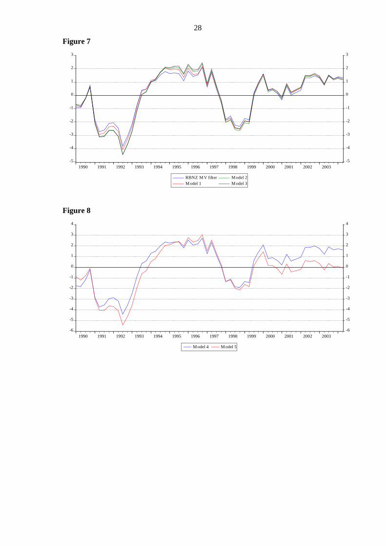
As we stated before, the weights placed to the structural residuals in the minimisation are the hyperparameters in our state-space model. Models 1, 2 and 3 assumed the weights imposed by the RBNZ’s MV filter where 2λ = 3λ = 2 We run the same models by allowing
the Kalman filter to choose the optimal weights. Because, we have 1 signal to noise ratio,
1λ , which is fixed at 1600, the variances of ute and cu
te can be estimated. Table 3 and
Figure 7 shows the results from this.
***Figure 7 about here***
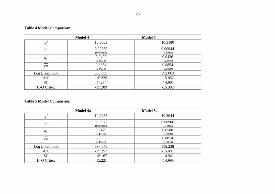
As we have shown above, the way the unobserved equilibrium values are treated can make some important difference to the final estimates. As a result of this conclusion, we now estimate the model in way that all unobserved trends and the coefficients are estimated simultaneously. All trend/equilibrium values are treated as unobserved variables.
Hence, we want to investigate this further. What we would like to do is to allow the unemployment trend and the capacity utilisation equilibrium to be unobserved variables, as well as the potential output. In fact, this is the approach taken in a recent paper by Benes and N’Diaye (2004). They estimate another class of multivariate filter, where both NAIRU and the potential output are treated as unobserved components.
We call these Models 4 and 5 respectively. In these models, we treat the equilibrium rate as unobserved variable in the following way and estimate the equilibrium capacity utilisation as a constant. The only difference between models 4 and 5 is that, in model 4, the coefficients are estimated and in model 5, they are imposed.
uttt guu 11 −− += (22)
tut
ut gg ϕ+= −1 (23)
The reason for treating the capacity utilisation as a constant, comes from the nature of the capacity utilisation survey. is sensible, as we believe the equilibrium capacity utilisation does not move around much. The trend unemployment on the other hand is a random walk with drift. We fix the hpyerparameter of the unemployment rate at 1600 as the output gap one. In other words, ),0(~ 2
,1 ut N σζ and tut N ϕλσϕ ),0(~ 22 .
Table 4 and 5 shows the estimates from these two kind of models. The difference between models 4 and 5 and models 4a and 4b is the imposition and estimation of the

12
hyperparameters. In these two tables, we do only focus on the equilibrium values, rather than the coefficients.
It is clear that the imposition or estimation of parameters make a big difference for the key equilibrium values. Models 4 and 4a, imposes the coefficients β
and γ
In these
models, the current equilibrium unemployment rates are estimated as 4.92 and 4.79 per cent respectively. In models 5 and 5a on the other hand, trend unemployment is much lower, hence the trend growth rate is much higher, above 0.9 per cent per quarter. The estimated equilibrium capacity utilisation is just under 89 per cent, almost identical to the RBNZ’s MV filter assumption.
***Table 4 about here*** ***Table 5 about here***
To highlight this difference, we plot the output gap estimated from models 4 and 5. Because the model 5 believes the fall in unemployment is due to trend, it gives almost no gap at the end of the sample. Model 4 on the other hand gives an output gap of around 1.5 per cent. We have to caution the reader with one thing about the model 5. In capacity utilisation equation, because we try to estimate the constant trend, as well as the coefficient and the variance (hence nothing is imposed), we get an extremely small coefficient. Hence that is also the reason, why output gap turns out to be zero in this model, despite a capacity utilisation, which is well above its estimated equilibrium value at the moment. Figure 8 shows the results from models 4 and 5
***Figure 8 about here***
It is clear that as the way we treat the equilibrium capacity utilisation does not matter, as long as it is treated as a constant.12 The equilibrium capacity utilisation is around 0.885 in most models. However, the trend unemployment rate depends on how we treat it and it also affects the final output gap estimates. In models 1, 2 and 3 we used a trend unemployment rate that was estimated outside the system. In Models 4 and 5, we estimated the trend unemployment rate as an unobserved variable. Figure 9 below compares the four different trend unemployment rates we used/estimated in this paper. An HP filtered trend, the MV filtered trend which uses the shill shortage series to augment an HP filter and two other equilibrium unemployment rate series, we estimated from models 4 and 5. Their evolutions are rather different. 13
***Figure 9 about here***
6 Revisions
In this section, we will look at the revision properties of the models we presented above. We believe this issue deserves more attention. This is as important as the inflation predicting ability of the output gap. Orphanides and van Norden (2003) have shown that no output gap model can escape from substantial revisions in ex-post. Hence, using the
12 If it is allowed to be a time varying equilibrium, then we get a different story. We do not follow that avenue for the reasons we stated above.
13 See Guy and Szeto (2004) for a Phillips curve based NAIRU estimates for New Zealand. They are completely different than the ones we estimated in this paper.
13
output gap in real time, can lead to wrong policy conclusions. (See Orphanides 2001 and Nelson and Nikolov 2003).
Previously, Twaddle (2002) argued that the revisions to the real time output gap estimates of the RBNZ’s MV filter are not as bad as an HP filter, but still very high. Furthermore, Graff (2004) states that the estimates for any given quarter do not converge to any final value, even after about 20 quarters. Those errors are around 2 per cent. However, as we argued above, the MV filter assumed no uncertainty in parameters, equilibrium values in the conditioning information. Therefore, once we allow uncertainty around these, the revisions can be substantially larger.
***Figure 10 about here***
Figure 10 above, shows the ex-post real time difference, in other words, the revisions to the output gap for the five different models, we estimated in this paper. The revisions are much smaller in models, where the potential output is the only unobserved variable. These results are similar to the Twaddle (2002). However, as we treat the other trends as unobserved variables as well, the revisions get much larger.
7 Future Directions and conclusions
The output gap concept plays a crucial role in the thinking and behaviour of many inflation targeting central banks. Yet, this concept is difficult to measure, due to the unobserved nature of the potential output. In addition, the real time estimates of the output gap are subject to massive revisions.
We have shown that the results of the LT approach can be dependent on the assumptions about the structural relations. In particular, the parameters and the equilibrium values assumed in the structural equations can make a significant difference to the output gap estimates. We also showed, though did not discuss in great detail, that the revision properties get worse, as the unobserved equilibrium values are not assumed to be known.
We argued that estimating the HPMV filter with the Kalman filter has many advantages over the iterative procedure proposed by LT. Based on different assumptions on trends and coefficients, the policy makers can see an envelope of output gap in ‘thick modelling’ sense.
References
Basdevant, O (2003), “On the Applications of Kalman Filter in Macroeconomic Time Series”, Reserve Bank of New Zealand Discussion papers Series, 2003/01
Basdevant, O, N Björksten and Ö Karagedikli (2004), “Estimating a time varying neutral-real interest rate for New Zealand, Reserve Bank of New Zealand Discussion papers Series, 2004/01
Benes, J and P N’Diaye (2004), “A Multivariate Filter for Measuring Potential Output and the NAIRU: Application to the Czech Republic”, IMF Working Paper WP/04/45.

14
Billmeier, A (2004), “Measuring a Roller Coaster: Evidence on the Finnish Output Gap”, IMF Working Paper WP/04/57.
Black, R et al (1997), “The Forecasting and Policy System; The core model”, Reserve Bank of New Zealand, Research Paper, 43
Boone, L (2000), "Comparing semi-structural methods to estimate unobserved variables: the HPMV and Kalman filter approaches," OECD Working Paper #240.
Butler, L (1996), “A Semi-Structural Method to Estimate Potential Output: Combining Economic Theory with a Time-Series Filter”, Bank of Canada Technical Report No 77.
Citu, F and J Twaddle (2003), “The output gap and its role in monetary policy decision-making”, Reserve Bank of New Zealand Bulletin, 66 (1), 5–14.
Clark, P K (1987), “The Cyclical Components of US Economic Activity”, Quarterly Journal of Economics 102(4), 797-814
Clark, P K (1989), “Trend reversion in real output and unemployment” Journal of Econometrics 40, 15-32.
Claus, I (2003), “Estimating potential output for New Zealand” Applied Economics, 2003, vol. 35, issue 7, pages 751-60
Claus, I, P Conway and A Scott (2000), “The Output Gap: Measurement, Comparisons and Assessment”, Reserve Bank of New Zealand Research Paper No 44, Wellington, June 2000.
Conway, P and B Hunt (1997), "Estimating potential output: a semi-structural approach," Reserve Bank of New Zealand Discussion Paper D97/9.
De Brouwer, G (1998), “Estimating Output Gaps”, Reserve Bank of Australia Research Discussion Paper 9809.
Elekdag, S (2001), “Kalman filter and its applications” Central Bank of Republic of Turkey, Discussion papers series.
Gerlach, S and F Smets (1997), “Output Gaps and Inflation: Unobserved Components Estimated for the G-7 Countries”, BIS mimeo
Gerlach, S and F Smets (1999), "Output gaps and monetary policy in the EMU area," European Economic Review, 43: 801-812.
Graff, M (2004), “Estimates of the output gap in real time: how well have we been doing?” Reserve Bank of New Zealand Discussion Papers Series, DP 2004/04
Granger, C and Y Jeon (2004), “Thick Modelling”, Economic Modelling, 21, pp 323-343.

15
Gruen, D, Robinson, T and A Stone (2002), “Output Gaps in Real Time: Are They reliable Enough to Use for Monetary Policy, Reserve Bank of Australia Discussion Paper, 2002/06
Hamilton, J (1995), “State-space models” in Engle, R F and D Mc Fadden (eds) Handbook of Econometrics Volume 4, 3041-3077
Hampton, T (2002), “Revisiting MV filter”, Reserve Bank of New Zealand, mimeo
Harvey, A (1989), “Forecasting, Structural Time Series Models and the Kalman Filter,” Cambridge University Press, Cambridge.
Harvey, A C (1985), "Trends and cycles in macroeconomic time series" Journal of Business and Economic Statistics 3: 216-27.
Harvey, A C (1985), “Trends and Cycles in Macroeconomic Time Series”, Journal of Business and Economic Statistics, 3, 216-227
Harvey, A C and A Jaeger (1993), “Detrending, Stylised Facts and the Business Cycle”, Journal of Applied Econometrics, 8, 231-247
Hodrick, R J and E Prescott (1997), “Post-war Business Cycles: An Empirical Investigation”, Journal of Money, Banking and Credit, 29, 1-16
Kalman, R E (1960), "A new approach to linear filtering and prediction problems," Journal of Basic Engineering, Transaction of the SAME, 59: 1551-1580.
Kuttner, K N (1994), “Estimating Potential Output as a Latent variable”, Journal of Business and Economic Statistics, 12(3) 361-368
Lansing, K (2002), “Can the Phillip Curve Help Forecast Inflation?” Federal Reserve Bank of San Francisco Economic Letter No 2002-29
Laxton, D and R Tetlow (1992), “A simple multivariate filter for the measurement of output gap”, Bank of Canada technical report, 59
Nelson, E and K Nikolov (2003), “UK Inflation in the 1970s and 1980s: the Role of Output Gap Mismeasurement”, Journal of Economics and Business, 55 (4), 353–370.
OECD (2000), “The Concept, Policy Use and Measurement of Structural Unemployment: Estimating a Time Varying NAIRU Across 21 OECD Countries,” Economics Department Working Paper 250
Okun, A (1962), “Potential GDP: Its measurement and significance”, Proceedings of the Business and Economics Statistics Section, American Statistical Association.
Orphanides, A and S van Norden (2003) The Reliability of Inflation Forecasts Based on Output Gap Estimates in Real Time, mimeo
Orphanides, A (2001) “Monetary policy rules based on real-time data,” American Economic Review 91, 964-985.
16
Orphanides, A (2003), “Historical Monetary Policy Analysis and the Taylor Rule”, Journal of Monetary Economics, 50 (5), 983–1022.
Orphanides, A, R D Porter, D Reifschneider, R Tetlow and F Finan (1999), "Errors in the measurement of the output gap and the design of monetary policy," Federal Reserve Board, Finance and Economics Discussion Series, 1999-45.
Orphanides, A and S van Norden (2002), “The Unreliability of Output-gap Estimates in Real Time”, Review of Economics and Statistics 84, 569–583.
Razzak, W (1997), “The Hodrick-Prescott technique: A Smoother versus a filter. An Application to New Zealand GDP”, Economics Letters, 75, 163–168.
Razzak, W (2002), “Monetary policy and forecasting inflation with and without the output gap”, Reserve Bank of New Zealand Discussion Paper 2002/03.
Robinson, T, Stone, A and M van Zyl (2003), “The Real-time Forecasting Performance of Phillips Curves”, Reserve Bank of Australia Discussion Paper, 2003/12
Scott, A (1996), “A Multivariate unobserved components model of the cyclical activity” Reserve Bank of Discussion Papers Series, 2000/04
St Amant, P and S van Norden (1998) “Measurement of the output gap: A discussion of recent research at the Bank of Canada”, Bank of Canada Technical Report No 79
Twaddle, J (2002), “The MV Filter and real-time data”, Reserve Bank of New Zealand, internal mimeo
Van Norden, S (2002), “Filtering for Current Analysis”, Bank of Canada Working Paper 2002-28.

17
Appendix A: The Kalman filter and the smoothed estimates14
Many dynamic models can be written and estimated in state-space form. The Kalman filter is the algorithm that generates the minimum mean square error forecasts for a given model in state space. If the errors are assumed to be Gaussian, the filter can then compute the log-likelihood function of the model. This enables the parameters to be estimated by using maximum likelihood methods.
For simplicity let us consider a measurement equation that has no fixed coefficients:
tttt XY ε+Γ=
(A1)
where Yt is a vector of measured variables, Γt is the state vector of unobserved variables, Xt is a matrix of parameters and εt~ ( )HN ,0 . The state equation is given as:
ttt η+Γ=Γ −1 (A2)
where ηt~ ( )QN ,0 .15
Let γt be the optimal estimator of Γt based on the observations up to and including Yt, γt|t−1
the estimator based on the information available in t−1, and γt|T the estimator based on the whole sample. We define the covariance matrix P of the state variable as follows:
( )( )
′−Γ−Γ= −−−−− 11111 ttttt EP γγ (A3)
The predicted estimate of the state variable in period t is defined as the optimal estimator based on information up to the period t−1, which is given by:
14 This section draws heavily on Basdevant (2003).
15 Q and H are referred to as the hyperparameters of the model, to distinguish them from the other parameters.

18
11| −− = ttt γγ
(A4)
while the covariance matrix of the estimator is:
( )( ) QPEP ttttttttt +=
′−Γ−Γ= −−−− 1111 γγ (A5)
The filtered estimate of the state variable in period t is defined as the optimal estimator based on information up to period t and is derived from the updating formulas of the Kalman filter:16
( ) ( )1|1
1|1|1| −−
−−− −+′′+= tttttttttttttt aXYHXPXXPγγ (A6)
and
( ) 1|1
1|1|1| −−
−−− +′′−= ttttttttttttt PXHXPXXPPP (A7)
The smoothed estimate of the state variable in period t is defined as the optimal estimator based on the whole set of information, i.e. on information up to period T (the last point of the sample). It is computed backwards from the last value of the earlier estimate γT|T=γT, PT|T=PT with the following updating relations:
( )tTtttTt P γγγγ ++= + |1*
| (A8)
( ) ′++= ++*
|1|1*
| tttTtttTt PPPPPP (A9)
where 1|1
* −+= tttt PPP .
Depending on the problem studied one can be interested in any one of those three estimates. In our particular case, looking at smoothed values is more appropriate, as the point is not to use the Kalman filter to produce forecasts but to give the most accurate information about the path followed by the time-varying coefficients. Therefore it is more informative to use the full dataset to derive each value of the state variables.
16 This estimator minimises the mean square errors when the expectation is taken over all the variables in the information set rather than being conditional on a particular set of values (see Harvey 1989 for a detailed discussion). Thus the conditional mean estimator, γt, is the minimum mean square estimator of Γt. This estimator is unconditionally unbiased and the unconditional covariance matrix of the estimator is the Pt matrix given by the Kalman filter.

19

Table 1 Estimation results of different capacity utilisation specifications*
OLS 2SLS OLS- Constant NA NA -0.0002
(0.002)
γ
0.629 (0.191)
0.858 (0.210)
1
2R
0.22 0.169 0.160
DW 0.34 0.42 0.47 *All standard errors are Newey-West heteroscedasticity consistent standard errors
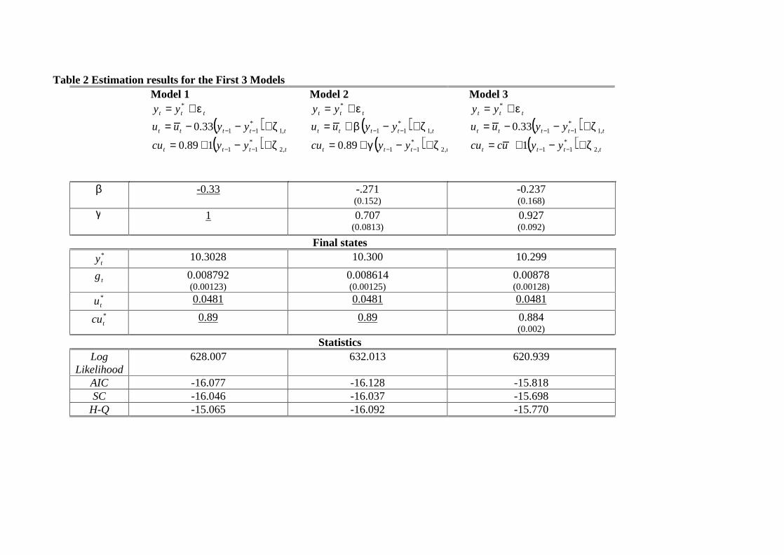
Table 2 Estimation results for the First 3 Models Model 1
ttt yy ε+= *
( ) ttttt yyuu ,1
*1133.0 ζ+−−= −−
( ) tttt yycu ,2*
11189.0 ζ+−+= −−
Model 2
ttt yy ε+= *
( ) ttttt yyuu ,1
*11 ζβ +−+= −−
( ) tttt yycu ,2*
1189.0 ζγ +−+= −−
Model 3
ttt yy ε+= *
( ) ttttt yyuu ,1
*1133.0 ζ+−−= −−
( ) tttt yyuccu ,2
*111 ζ+−+= −−
β
-0.33
-.271 (0.152)
-0.237 (0.168)
γ
1
0.707 (0.0813)
0.927 (0.092)
Final states *ty 10.3028 10.300 10.299
tg 0.008792 (0.00123)
0.008614 (0.00125)
0.00878 (0.00128)
*tu 0.0481
0.0481
0.0481
*tcu 0.89
0.89
0.884 (0.002)
Statistics Log
Likelihood
628.007 632.013 620.939
AIC -16.077 -16.128 -15.818 SC -16.046 -16.037 -15.698
H-Q -15.065 -16.092 -15.770

22
Table 3 Estimation results with different hyper parameters Model 1a Model 2a Model 3a
β
-0.33
-.323 (0.040)
-0.318 (0.046)
γ
1
0.547 (0.124)
0.675 (0.151)
Final states *ty 10.3052 10.3050 10.299
tg 0.009028 (0.00141)
0.008958 (0.00141)
0.00897 (0.00141)
*tu 0.0481
0.0481
0.0481
*tcu 0.89
0.89
0.884 (0.003)
Statistics Log
Likelihood
672.738 632.013 666.517
AIC -17.172 -17.279 -16.936 SC -17.082 -17.128 -16.755
H-Q -17.136 -17.219 -16.863
23
Table 4 Model Comparison
Model 4 Model 5 *ty 10.3003 10.3180
tg 0.00889 (0.00015)
0.00944 (0.0018)
*tu 0.0492
(0.0038) 0.0436 (0.0048)
cu 0.8854 (0.0034)
0.8854 (0.0029)
Log Likelihood 600.689 592.063 AIC -15.325 -15.052 SC -15234 -14.901
H-Q Criter. -15.289 -15.992
Table 5 Model Comparison
Model 4a Model 5a *ty 10.2985 10.3044
tg 0.00873 (0.00016)
0.00906 (0.0015)
*tu 0.0479
(0.0039) 0.0508 (0.0040)
cu 0.8853 (0.0025)
0.8854 (0.0063)
Log Likelihood 598.048 589.238 AIC -15.257 -15.031 SC -15.167 -14.941
H-Q Criter. -15.221 -14.995

24

Figure 1: Revisions to the HP filtered unemployment gap.
-1.2
-0.8
-0.4
0.0
0.4
0.8
1.2
1.6
2.0
2.4
-1.2
-0.8
-0.4
0.0
0.4
0.8
1.2
1.6
2.0
2.4
1990 1991 1992 1993 1994 1995 1996 1997 1998 1999 2000 2001 2002
DIFFERENCE_UGAPNZ
Figure 2 Skill shortage survey series and its assumed equilibrium
-40
-30
-20
-10
0
10
20
30
40
50
60
-40
-30
-20
-10
0
10
20
30
40
50
60
1990 1991 1992 1993 1994 1995 1996 1997 1998 1999 2000 2001 2002 2003
STAFF_HPTREND STAFFSHORT STAFF_MEAN
26
Figure 3
Figure 4 Time varying equilibrium of the capacity utilisation
.83
.84
.85
.86
.87
.88
.89
.90
.91
.92
.83
.84
.85
.86
.87
.88
.89
.90
.91
.92
1983 1984 1985 1986 1987 1988 1989 1990 1991 1992 1993 1994 1995 1996 1997 1998 1999 2000 2001 2002 2003
Capacity utilisationMV filter trend
HP-1600HP-30000
-.04
-.03
-.02
-.01
.00
.01
.02
.03
.04
-.04
-.03
-.02
-.01
.00
.01
.02
.03
.04
85 86 87 88 89 90 91 92 93 94 95 96 97 98 99 00 01 02 03
CU_RESID_2LS CU_RESID_OLS CU_RESID_OLS2

27
Figure 5 HPMV filtered output gaps and the Bank’s MV filter.
-5
-4
-3
-2
-1
0
1
2
3
-5
-4
-3
-2
-1
0
1
2
3
1990 1991 1992 1993 1994 1995 1996 1997 1998 1999 2000 2001 2002 2003
RBNZ M V filterM odel 1
M odel 2M odel 3
Figure 6 Mean out put gap estimate and 1 standard errors
-5
-4
-3
-2
-1
0
1
2
3
-5
-4
-3
-2
-1
0
1
2
3
1990 1991 1992 1993 1994 1995 1996 1997 1998 1999 2000 2001 2002 2003
+ 1 std devmean gap estimate- 1 std dev
28
Figure 7
-5
-4
-3
-2
-1
0
1
2
3
-5
-4
-3
-2
-1
0
1
2
3
1990 1991 1992 1993 1994 1995 1996 1997 1998 1999 2000 2001 2002 2003
RBNZ M V filterM odel 1
M odel 2M odel 3
Figure 8
-6
-5
-4
-3
-2
-1
0
1
2
3
4
-6
-5
-4
-3
-2
-1
0
1
2
3
4
1990 1991 1992 1993 1994 1995 1996 1997 1998 1999 2000 2001 2002 2003
M odel 4 M odel 5

29
Figure 9 Equilibrium Unemployment rates
.04
.05
.06
.07
.08
.09
.10
.04
.05
.06
.07
.08
.09
.10
1990 1991 1992 1993 1994 1995 1996 1997 1998 1999 2000 2001 2002 2003
MV filtred trend unempHP filtered trend unemp
trend unemp from Model 4trend unemp from Model 5
Figure 10 Revisions to 5 models presented
-3
-2
-1
0
1
2
3
4
5
-3
-2
-1
0
1
2
3
4
5
1990 1991 1992 1993 1994 1995 1996 1997 1998 1999 2000 2001 2002 2003
revisions to M odel 1revisions to M odel 2revisions to M odel 3
revisions to M odel 4revisions to M odel 5