Estimating the Manifold Parameters of One Dimensional

Estimating the Manifold Parameters of One-Dimensional Arrays of Sensors page 1 of 17

Estimating the Manifold Parameters ofOne Dimensional Arrays of Sensors.c

byI. DACOS A. MANIKAS PhD, DIC PhD, DICand

Department of Electrical and Electronic Engineering,Imperial College of Science, Technology and Medicine,

University of London.London, SW7 2BT.

Journal of The Franklin Institute,Engineering and Applied Mathematics,

Vol. 332B, No.3, pp.307-332, 1995.

Permission to publish this abstract separately is granted.

Abstract: In the direction finding problem successful application of the signal-subspace type algorithmsrequires the use of the concept of the . However, despite the importance of this concept,array manifoldsignal-subspace algorithms use the in a primitive way, since its andarray manifold propertiesparameters remain unknown.In this paper an attempt is made to identify, estimate and study the most important parameters of themanifold of a general linear array of sensors by using differential geometry. Initially the generalN

theory is developed and expressions are derived for the , and of thecurvatures coordinate vectorscomplex manifold-curve. Then the and of the manifold of linear arrays areshape orientationinvestigated. It is shown that the manifold-curve of a linear array of omnidirectional sensors has theshape of a complex circular on a sphere in the complex space while a measure of itshyperhelix CN

orientation can be provided by introducing the concept of the . Analytical expressionsinclination anglefor the curvatures, manifold radii, number of windings etc. are also provided.Finally, it is shown that, if the array is symmetrical, i.e. all sensors are symmetrically located withrespect to the array centroid, the manifold is equivalent to a on acomplex hyperhelix real hyperhelixsphere in .RN

I. Dacos was formerly with Imperial College of Science, Technology and Medicine and is now with Hellenic Air ForceAcademy, Dekelia, Athens, Greece.

A. Manikas is with the Department of Electrical and Electronic Engineering, Imperial College of Science Technology andMedicine, University of London, London SW7 2BT, United Kingdom.

One of the authors, I. Dacos, is indebted to the Onassis Foundation for the Research Scholarship they have awarded him.


I. INTRODUCTION

In the array processing problem the most important class of techniques currently being examinedare the so called Signal Subspace Techniques. The Signal Subspace class of techniques uses, directly orindirectly, the concept of the . For instance, the MuSIC algorithm [1] can be viewed asarray manifoldan algorithm which finds the intersection of the with the , and ASPECTsignal subspace array manifold[3] can be viewed as an algorithm which starts with an initial guess of the signal subspace and thenmoves towards the true signal subspace by using some function of the and derivatives of the1st 2ndarray manifold. However, in both these algorithms, the concept of the array manifold has been used inan elementary way, since its properties and parameters remain unknown. This concept directly suggeststhe use of differential geometry [4]. However, the application of differential geometry, which is an olddesire of researchers working in this area, although is obviously suggested by the concept of the arraymanifold, has so far been prevented by its difficult and purely mathematical nature.

In this paper an attempt has been made to identify the parameters which demonstrate potentialbenefits for identifying the shape and orientation of the manifold of a general linear array of sensors.The estimation of those parameters is a central task of this paper hoping that they will provide thenecessary basis for future exploitation of the array processing problem.

One of the initial aims of the work reported in this paper was also to extend some concepts ofordinary differential geometry of real space or into the complex space This extension thenR R C� � N.

makes it possible to treat the general case of an arbitrary number of sensors . Thus, given an array of N N

sensors and a planar wave impinging on the array from some direction , there exists a ² Á ³� � N-

dimensional vector representing the array response in that direction. This vector is said to be theaSource-Position-Vector manifold vector (SPV) or and it has the following form:

( ) ( ) ( ) ( )a a~ � � � � � �, g , j k , 1_~ p cexpF r T G

where a 3 matrix with columns the three dimensional sensor-locations measuredr ~ Á Á ² d 5³" #� � �% & 'T

in half-wavelengths, ( ) is the wavenumber vector, andk k _ _~ Á� � ~ Á Á� � � � � �" #cos cos sin cos sin T

g ( ) is the complex vector with elements the gain and phase response of the array elements. It can be� �Á

seen from the above equation that the element of the vector ( ) represents the phase delayi j k_th c Ár T� �

at the sensor of the incident signal from the direction relative to a reference point. It will be shown�!� �

later that it is convenient to choose the reference point at the array centroid.

It is clear from that the source position vector for a particular direction contains all theEquation 1 ainformation about the geometry involved when a wave is incident on the array from that direction.Consider the source position vector (or manifold vector) corresponding to the direction , where isa � �

for instance the azimuth angle. Rewrite as ( ). Next, record the locus of the vector ( ) as a functiona a a� �

of . This locus is a continuum (i.e. a curve) lying in a and is� 1-dimensional dimensional spaceN-

known as the . If the direction is given by two parameters ( ) where is the azimutharray manifold ,� � �

and is the elevation angle, then the continuum becomes , i.e. a surface, etc. The � 2-dimensional arraymanifold can be calculated (and stored) from only the knowledge of the locations and directionalcharacteristics of the sensors. Thus, according to Schmidht [1], the completelyarray manifoldcharacterizes any array and provides a representation of the real array into complexN-dimensionalspace. This is the state of knowledge relating to the concept of the .array manifold

In this paper attention is focused on the of a linear array of sensors, where the onlymanifoldparameter involved is the azimuth angle. In this case the manifold vector is simplified to

a a~ ² ³ ~ ² ³ p c� � � � g j . 2expF �% cos G ( )

where is the real vector with elements the sensor positions in half wavelength. To simplify the�%notation the vector will be denoted as . Furthermore, if the array has omnidirectional sensors,� �%

Equation 2 is simplified to


a a~ ² ³ ~ c� � � j 3expF r cos G ( )

It is clear for that, in an “azimuth only" system, where there is no other parameter apartEquation 2from the azimuth angle, the manifold vector continuum a is a curve in . This curve, according to_²�³ CN

[1], behaves like a in the complex - space.snake dimensional N

The organization of the paper is as follows: In Section II the concepts of differential geometry are extended to the complex space . The setCN

of , the matrix, the matrix [2] and a number of important properties arecurvatures Frame Cartanderived for a general manifold. In Section III the concepts from section II are used and the shape of the manifold of a linear arrayof omnidirectional sensors is shown to be a complex . For this thecircular hyperhelix hyperhelix,curvatures length, windings coordinate vectors, the the number of and the are derived. Special cases ofuniform arrays symmetrical arrays and are also considered. In Section IV the manifold radii vector is introduced and the manifold inclination is proposed as ameasure of the manifold orientation in the complex space.N-dimensional In Section V it is shown that the manifolds of the widely used arrays which are symmetrical withrespect to the array centroid can be defined using a The analysis shows that thisreal representation.class of arrays is important since the dimensionality is reduced from to N- N-dimensional complex space dimensional real space. In Section VI, the main results obtained are summarized.

NotationN Number of sensors . Euclidean norm+ +( ) transpose ( ) determinant. det . T

( ) transpose conjugate ( ) trace. Tr . H

Re .( ) real part Hadamard productp

Im .( ) imaginary part identity matrixc fix .( ) integer part zero matrixi

II. DEVELOPMENT OF THE GENERAL THEORY(Extension of ordinary differential geometry in R or R to C )� � N

In this section a number of important parameters and properties of the are definedarray manifold and analytically estimated. Since only one directional parameter is involved, the azimuth angle , and�

the number of sensors is , the array manifold is a curve imbedded in complex dimensions. If theN N

sensors are omnidirectional, then the manifold curve lies on the complex sphere withN-dimensionalradius i.e.lN

( ) ( )+ +a � ~ lN D� 4

continuously differentiable orthonormal system ofThe first step in the development is to fix a and coordinates orthonormality continuously along a running point of the curve. The of this u�

differentiable frame relies on the fact that a vector continuum with constant magnitude is orthogonalu�

to its tangent. In the case of the unity magnitude complex vector continuums corresponding to arrayu� manifold coordinate vectors the above is true for the broad class of arrays which are symmetrical withrespect to their centroids. shows an example of a symmetrical and a non-symmetrical array.Figure 1However, if the array is not symmetrical, the orthogonality is no longer valid. This situation leads to thedefinition of and of two complex vectors of unity magnitude.wide-sense narrow-sense orthonormality The formal definitions are as follows:

wide sense orthonormality Re 0 5( ( )u u� �H ³ ~ � £ �

narrow sense orthonormality 0 6u u� �H ~ � £ � ( )


Thus, for a general linear array (i.e. an array for which the sensors are non-symmetrical withrespect to the array centroid), the will be used. This will be simplified towide-sense orthogonalitynarrow-sense for symmetrical arrays. Next, the arc length is introduced as a parameter alternative to .s �

System of coordinates and Curvatures As was mentioned above the first objective is to fix a continuously differentiable and orthonormalsystem of coordinates u wide-sense orthogonality_� along a running point of the curve. We will use the since symmetrical arrays may be considered as a special case of non-symmetrical arrays. The arc lengthalong the manifold is defined by

dq 7d q

dq ~( ) ( )

a( )_� � j j

�

�

in which case ( ) a( ) ( )_ s 8dsd

À~ ~� �

�+ +À

where throughout this paper is used to denote differentiation with respect to parameter while is. ! !�

Z

used to denote differentiation with respect to . Notice that the arc length, , is a much more natural way sof parametrizing a curve as compared with since it corresponds to actual physical length in�

multidimensional space. Another advantage of using as a parameter is that the resulting tangentsvector to the curve always has unit length. That is

a ( )_a( )_+ +Z À

~ ~ ~ ~ D 1 9d s

dsj j k k i id_

ddd

s

a( )a( )_( )

�

�

�

�

� À �

In order to fix the continuously differentiable system of coordinates, the unit length tangent vector of a( ) with respect to is taken as . Then_ � s u_�

s 10u�( ) a ( )_~ Z

Later, it will become apparent that by a judicious choice of the origin of the coordinates on thearray line, the vector ( ) can always be made orthogonal to ( ) in the narrow sense.u� s s a Because ( ) the vector+ +u� s const, ~

( ) , ( )u� s 11~uu�Z

�Z

( )( )ss+ +

is of unit length and orthogonal to ( ) in the wide sense i.e.,u� s

( ) ( ) ( )Re s s 0 126 7u u� �H ~

This can be regarded as the unit vector. It is noted that ( ) is collinear withsecond coordinate d su�

u� � �( ) Hence, there exists a scalar ( ) such thats . k k s~

( ) ( ) ( )d s k s ds 13u u� � �~

so that ( ) ( ) k s 14� �Z~ + +u

The scalar is defined as the . The vector can be chosen as the unit-length vector in k first curvature� �uthe direction ( ) ( ) Indeed, s k s .u u�

Z� �b

Re Re k Re k( ) ( ) ( )u u u u u u u� � �Z Z

� � � � �H H H

� ~ b ~ b ~6 7 Re k Re k k 0 15~ c b ~ c b ~( ) ( ) ( )u u u u� � �

Z� � � �

H H6 7


Re Re k Re 0 16and ( ) ( ) ( ) ( )u u u u u u u� � �� Z ZH H H~ ~6 7b ~

In ( ) stems from the fact that is of constant length and hence has no realEquation 16, Re 0u u u u� �Z

� H ~ �

Z

component along . Hence, there exists a scalar ( ) satisfyingu� k k s� �~

( ) ( )d k k ds 17u u u� � � � �~ c b

so that ( )k k 18� � ��

Z~ b+ +u u

The scalar is defined as the sometimes called the . It is possible to proceed k second curvature, torsion�

by fixing ( ) as the unit length vector in the direction of the vector ( ) ( ) :u u u� � ��Zs s k sb

( ) ( ) ( ) ( ) ( )_Re Re u k Re Re 0 19u u u u u u u� � � � �� Z ZH H HH

~ b ~ ~�

Re Re u k Re k( ) ( ( )_u u u u u� � � �� Z ZH HH

~ b ~ c b ~�³

Re k k k 0 20~ c c b b ~6 7( ) ( )� � � � � �u u uH

and Re Re k Re Re Re k 0 21( ( ) ( ) ( ) ( ) ( )u u u u u u u u u u� � � � � ��

Z ZH H H HH³ ~ b ~ c ~ c ~

Hence, there exists a scalar ( ) , called the ( ) satisfyingk k s third curvature k k s� � � �~ ~

d k k ds 22u u u� � � � �~ c b( ) ( )

k k 23¬ ~ b� � ��Z+ +u u ( )

and, in general, ( )u u u�

Z� � � � � �~ c bk k 24- - b�

k k 25� � � �c��Z~ b+ +u u- ( )

, k 0 26u� � �b À

~ £u u�c�Z

�c� �c�

�c�

kk - ( )

If the number of sensors is (i.e. the manifold vector can be described by real components) thenN 2N

at most manifold curvatures can be defined. However, if there exists an index such� � � � �N Nc c�

that the procedure is prematurely terminated which implies that k 0, k k ... .�c� � �b�~ ~ ~ ~ �

Frame and Cartan Matrix Consider next that the point of interest is a point on the array manifold where and at s 0~°

which the ( ) is unknown. Consider, however, that the set of coordinateset of coordinate vectors s o

vectors is known at ( ) ( ) Then ( ) can be found by using a simples i.e. known. s ~ � � ~� ~ � o o

continuous differentiable real transformation matrix function ( )` s , i.e.

s . s 27o o `( ) ( ) ( ) ( )~ �

with ( ) ( ) ( )` � ~ c 28identity matrix

The continuously differentiable transformation matrix ( ) is called , and this is a` s frame matrixnonsingular matrix.

Now the question under consideration is how the is related to the curvatures of theframe matrixmanifold. Firstly, define the skew-symmetric matrix with elements the curvatures of thed d d ]

manifold as :


s 29

0 k s 0 0 0k s 0 k s 0 0

0 k s 0 k s .........0 0 k s 0

..........0 k s 0 k s0 0 k s 0

]( ) ( )

( )( ) ( )

( ) ( )( )

( ) ( )( )

�

c

c

c

c

x {z }z }z }z }z }z }z }z }y |

�

� �

� �

�

� � �

�

- d-

d-

where is the number of manifold coordinate vectors. If there is no sensor located at the arrayd � �N

centroid, the parameter (dimensionality of the above matrix or number of coordinate vectors) is equald to where is the number of sensors in symmetrical pairs. Otherwise, is equal to � � �N Nc cm, m d m .c

For instance, for the symmetrical array shown in while for the non-symmetrical arrayFigure-1a, ,� ~ �

of Figure-1b, The matrix ( ) is defined as the matrix of the manifold By using the� ~ �À ] s Cartan .Cartan Equation 24 matrix, can be written in a compact form as follows

( ) ( ) ( ) ( ) ( ) ( ) ( ) s s . s . s . s 30o o ] o ` ]Z ~ ~ �

where ( ) ( ) ( ) ( ) ( ) o s s , s , ... , s 31~ ¶ ·u u u� � d

i.e. ( ) is a continuously differentiable matrix formed by the manifold ando s d coordinate vectorsN d

oZ Z Z Z

� �( ) ( ) ( ) ( ) ( )s s , s , ... , s 32~ ¶ ·u u ud

The can always be written as a function of the ( ) Indeed, due toCartan matrix frame matrix s . `

Equations 27 30, sand ( ) satisfies the differential equation`

s s . s 33` ` ]Z( ) ( ) ( ) ( )~

From the above equation one can deduce that

( ) ( ) ( ) ( ) ( ) ( )] ` ` ` `s s . s s . s 34~ ~c� Z ZT

The matrix is also related to the matrix of manifold coordinate vectors ( ), as follows:Cartan o

]( ) ( ) ( ) ( ) ( ) ( ) ( ) ( ) ( ) ( ) ( )

( ) ( )

s s . s s .Re . . s Re s . . s

s s

~ ~ � � ~ � �

§ § §

` ` ` o o ` ` o o `

co o

c� Z c� Z c� Z6 7 6 7H H

H

Z

s Re s s 35¬ ~] o o( ) ( ) ( ) ( )6 7 H Z

By using the above concepts, the shape of the manifold of a general linear array of isotropicN

sensors will be investigated in the following section.

III. SHAPE of the ARRAY MANIFOLD for a general LINEAR ARRAY

In this section the shape of the of a linear array of isotropic sensors is investigatedarray manifoldby using the theory developed in the previous section. The theory is valid for any complex manifold

curve which can be described by an expression similar to ( ) The main resultsa � � �~ cexpF j .rcos Gare presented in the following theorem:

Theorem 1.a) The manifold of a linear array with omnidirectional sensors is a circular lying onN hyperhelix

the complex dimensional sphere with radius N- Nl .


b) The curvatures of this hyperhelix depend on the lower order curvatures, the number of sensorsand their relative spacing and can be estimated by the following recursive equation:

k 1 b , k 0 36~� � � �

~�

� � �~ c £1k k . . .k

n

n- - n

,n -� � � �- k k�fix( ) 1i

2 b

b�( ) ( )r

where the coefficients are given by: b b k b i 37� � � � � �

�� ,n - ,n - ,n- -~ b � 2 ( )

with initial conditions k b for i b k 38~

� � ��~ Â ~ � Â+ +r , 1 1 ( )2,2 1

2~

and the vector with elements the normalized sensor positions 39~r ~ ~r

r+ + ( )

c) The number of windings odd or the number of half windings even of the hyperhelix is( ) ( )N N

n 40$ ~2 r

l+ +�$

( )

where l is the positive number which corresponds to the 1 root of the function$ ( )Nc th

F s Tr e 41$ ( ) ( )~ F G]]

with denoting the Cartan matrix of the array manifold.]

Corollary 1: The manifolds of linear arrays are arcs (closed hyperhelices)uniform hypercircular .

Theorem-1 Deductions : The essential feature of the manifold of any linear array of omnidirectional sensors, which isrevealed by Theorem-1, is that its curvatures, and hence its Cartan matrix , are constant, or]

equivalently, independent of directions. Furthermore, the independence of the from the absolute spacings (and hence thecurvaturesindependence of the from the absolute spacings) in conjunction with the dependence ofwinding lengththe on the absolute spacings, reveals that two linear arrays and with sensors atmanifold length ( ) ( ) � �

positions given by the vectors and with r r r r(1) (2) ( ) ( ) � �~ �

Î have manifolds which fit upon each other andÎ the associated number of windings ( or half-windings) satisfy the following relationship

where is a scalar constant ( )nn

42( )

( )

�

$

�

$

, ~ � �

It is worth noting that the definition of is restricted to linear arrays with an half winding evennumber of sensors. Thus, for an array with number of sensors, the function ( ) doesodd F Equation-41$

not generally have a root at the point on the manifold which corresponds to half the length of onemanifold winding.Similarly, the definition of one is restricted to linear arrays with number of sensors. Thus,winding oddfor an array with number of sensors, the function does not generally have a root at the point oneven F $

the manifold which corresponds to the length of a twice half manifold winding.

Finally, a careful examination of the analysis presented in Appendix-1 indicates that at broadsidethe coordinate vectors ( ) ( ) ( ) are real vectors while the coordinate vectors ( ) ( )u u u u u2 4 6 3s , s , s etc s , s ,�

u5( ) are imaginary vectors. Furthermore, the matrices ( ), ( ) and ( ), which are defined ass etc s s so o ore im

followso( ) ( ) ( ) ( ) ( )s = s , s , s ,... (s) 43´ Á µu u u� 2 3 ud

ore( ) ( ) ( ) ( ) ( )s = s , s , s , ... , 44´ ² ³µÂu u u2 4 6 uo

oim( ) ( ) ( ) ( ) ( )s = s , s , s , ... u (s) 45´ Á µÂu u u1 3 5 f

with and � ~ ��% � ~ ��% b �4 5 4 5� �c��


satisfy the following relationships:ore re( ) ( ) ( )s s 46H

o c~ oim im( ) ( ) ( )s s 47H

o c~

o ore im re im( ) ( ) ( ) ( ) ( )s s , Re s s 48H Ho o~° ~i i !

9� 9� ! !a( ) ( ) a( ) ( ) ( )s s = s s 49H Ho oim � Á ~° �T T

��

Evaluating the Curvatures of Uniform Linear Array Manifolds: Having presented Theorem-1, we now can calculate all the curvatures of any linear array. Forinstance, in Table-1, the four first curvatures are tabulated for arrays with 3 to 10 elements chosen fromthe popular class of uniform linear arrays with half-wavelength spacing. Furthermore, in theFigure 2four first curvatures are shown versus the number of elements in the array. It is apparent from Figure 2that the curvatures are monotically decreasing as the number of elements exceeds twice the order of thecurvature.

Table-1: The First Four Curvatures of the Manifold of Uniform Linear Arrays5 ~ � 5 ~ � 5 ~ 5 ~ 5 ~ � 5 ~ � 5 ~ 5 ~ ��

�À�� À�� À� � �� À� À�� À�� À��

�

�

+ +� .�

�

�À�� À�� À�� À� �À� � �À�� À�� À��

� �À�� À�� À�� À� � �À� � �À�� À��

c �À�� À�� À� �À�� À�� À�� À��

c c � �À�� À�� À�� À� � �À��

�

�

�

�

It is important to point out that, because the manifold has constant (first) and lies onprincipal curvaturea sphere with radius , a lower limit for islN k�

( )k 50� � 1lN

The above relation also stems from the following inner product a in conjunction with theHu� expression ( ) ( ) ( )a a a a aH H H H HHu u u u u u u� � � ��

Z ZZ Z Z~ ~b ¬ b 51

That is,

a ( ) ( )H H H Hu u u u u� � �� Z Z~ ~ c ~ � c ~ c ² ³1 1 1 1

k k k k

� � � �a a6 7 1 52

¬ � � k 53+ + + + la . ( )u� �1 1 1k k� �

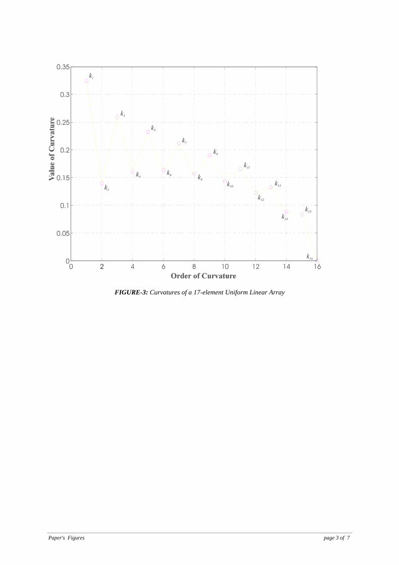
¬ ¬N .1� lN

Figure 3, 17In the curvatures of a element uniform linear array of sensors are shown to followc

a fading oscillating pattern.

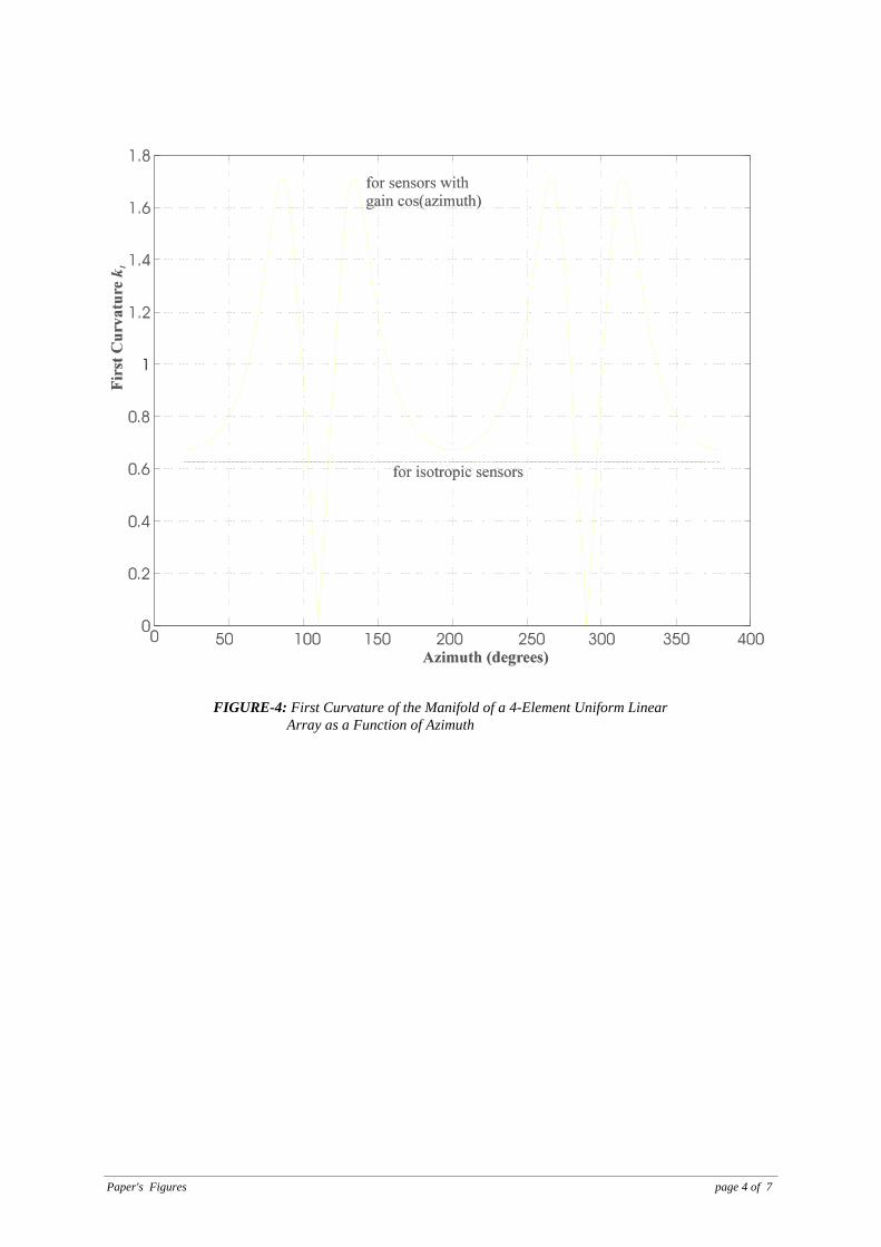
It should be noted that the manifolds of non omnidirectional linear arrays are not hyperhelices.The first curvature of the manifold of such arrays depends both on the relative spacing and the two firstderivatives of each elemental pattern In the case of the manifold of a element uniform linearg . 4� !� c

array with non-isotropic but identical sensors with directional pattern is ( ) the variation withg cos � � �~

the azimuth of the first curvature is shown in . The constant first curvature of the correspondingFigure 4isotropic array is also shown in the same figure. It is seen that there exist two bearings where the firstcurvature vanishes. From the variation of the first curvature it is possible to deduce the geometricalobject to which the manifold best fits. In the case considered, it is apparent that the effect of thesinusoidal elemental pattern is to deform the hyperhelix to a geometrical figure resembling an “ "eightwith a double point at the origin of the coordinates of CN.


IV. ORIENTATION OF THE MANIFOLD of a LINEAR ARRAY

In the previous section it has been shown that the shape of the manifold of a general linear array ofomnidirectional sensors is a complex circular lying on the complex hyperhelix N-dimensional spherewith radius lN. In this section an attempt is made to identify the orientation of the array manifold(hyperhelix) on the complex -dim space. Therefore it is necessary to establish a measure of theNorientation of the manifold curve in the complex observation space .CN

It is proposed to use the new concept of as a measure of the manifoldarray inclination angleorientation, which is intuitively defined as follows:

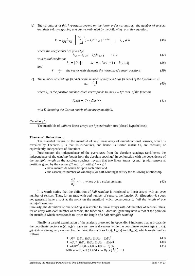
Definition- inclination angle:The inclination angle of the manifold of a linear array is the angle formed between any manifold

vector s and the space i.e. the space spanned by the columns of the matrixa( ) B !osub² ³ , osub² ³ ÀÀÀÁ= ,( ) ( ) ( )" # s , s , s ,u u u2 �

up to the -coordinate vector5

that is, s s 54cos( ) ( ) ( ) ( ) ~ m 1N

a aH josub

where is the projection operator onto josub B !osub² ³

Some insight to the above definition may be gained by the following sequence of arguments whichinvolves the presentation of a Lemma, Lemma-1, as well as the definition of the manifold radii.Having defined the matrix as a submatrix of and because of the orhonormality ofo osub re² ³ ² ³

columns of the matrix it is apparent that can be rewritten asore² ³ ² ³see Equation 46 Equation 54 follows:

( ) ( ) ( ) ( ( ) ( ) ( )cos ~ ~ ³m o �1 1N N a a as s s s 55H HHo osub sub

N

� ~ ��#��

u��

It is clear from the above equation that inclination angle is directly related to the inner products of amanifold vector with the coordinate vectors , , ... etc.u u u2 4 6,

Lemma-1, which is proved in Appendix-2, provides expressions for the above inner products.

Lemma-1 For a linear array of sensors, the interior products of a manifold vector with its d coordinatevectors are constant which depend on the array manifold curvatures and are given by the followingexpressions

aH u� ~ ² ³

c �� ~ �

c �� #��

~��

1k

k

k

�

�

�

n even

n odd

�c

�c

�

�

n

n

56

��

Re 57

( ) ( )if )if

aHu� ~� � ~ �� ~ � ²

� � ~ �� ~° �H i.e. there is a sensor at the array centroid, that is =oddÁ 5

It is obvious from Lemma-1 that curvature of odd order, i.e. , , , ... etc., cannot be zero.k k k1 3 5

Furthermore, the interior products of the manifold vector with the even-indexed coordinate vectorscorrespond to inverse curvatures

s s = , , ,...., , ..., 58a( ) ( ) [ ( )H.ore c c c µ1k k k k k k

k k k k

k � � � � �

� � � ��

��

�

�

even

odd

�c

�c

�

�

or a(s) ( ) [ 0, ( )9� !H.o s = , , , , ,...., , ... 59c � c � c �Á � µ�k k k k k k

k k k k

k � � � � �

� � � ��

��

�

�

even

odd

�c

�c

�

�

This leads to the following definition:


Definition- manifold radii:For a linear array of N sensors, with m sensors in symmetrical pairs, the quantities

R and R , i even, 60� �~ ~1k

k

k �

��

��

�

�

even

-

odd

-

�

�

2

1 ( )

are said to be the manifold radii while the vector R , formed by the manifold radii as follows

R~

~��

" #

" #

�Á c �Á c �Á ÀÀÀÁ �Á c ~ c

�Á c Á �Á c Á �Á ÀÀÀÁ �Á c Á � ~ c c

R , R , R d 2N m,

R R R d 2N m 1,

� � �

� � �c�

T

T

no sensor at array centroid

otherwise

( )61

is said to be the manifold radii vector.

From in conjunction with , the inclination angle can be rewritten as followsEquation-55 Equation-61

cos( ) where is the vector formed by the first elements of vector ~+ +lR "�

"�N

9 5 9

which reveals that the is constant depending only on the norm of a sub-vector of theinclinationmanifold radii vector and the number of sensors, that is,

( )¬ ~ ~arccosJ K const. 62+ +lR

"�

N

V. SYMMETRICAL versus NON-SYMMETRICAL ARRAYS

Initially, it is important to give special attention to the properties of the manifold of linearsymmetrical arrays, of which the popular uniform arrays are members. The manifolds of symmetricalarrays are shown to admit This can be seen intuitively from the fact that thereal representation. components of a manifold vector of symmetrical arrays exist in conjugate pairs. In addition, in theabsence of weighting, such arrays have purely real array patterns. The following theorem is necessary inorder to obtain analytically the real representation.

Theorem 2Consider a linear array of N sensors with m sensors in symmetrical pairs and with representing itsRd-dimensional manifold radii vector

a) ( ) The complex array manifold vector s can be expressed as a function of the curvatures, theaarc length and the coordinate vectors as follows

e 63a( ) ( ) ( )� ~ �o� �+ + !r �ccos ] R

b) ( )If m=N or m=N 1 , that is if the array is a symmetrical linear array, then there is a c real N-

dimensional hyperhelix with differential geometry properties equivalent to those of the complexN-dimensional manifold of the array. The real manifold vector associated with this realhyperhelix is given

e 64 a�( ) ( )� ~ � �+ + !r �ccos ]R

and can be regarded as the real representation of the manifold of a symmetrical array in 9N.

Proof


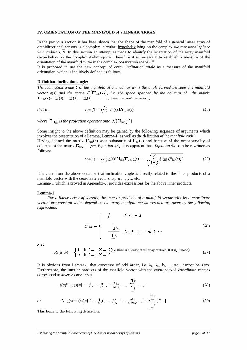
a) The manifold vector of a linear array can be expressed as a function of the , thearc length scurvatures coordinate vectors and the at . By using the first part of the Lemma-1 and because ~ �

the even indexed columns of are orthonormal, it can be found thato narrow sense

( ) ( ) ( ) ( ) ( ) ( )a s s s e 65~ ~ � ~ �o o ` oR R R ]

r 66where ( ) ~ ² ³ ~� � �+ + !� c cos

b) Choosing the columns of ( ) at to be the standard orthonormalN Ncoordinate vectors 6 7o � ~ �

basis in , i.e. setting ( ) and expressing as a function of via where R , s Equation , No � ~ �c � � ~

( ) is taken along the array axis, the of a real having thes Equation-64 dimensional hyperhelix~ � N-

samelength identical and with these of the complex manifold , can becurvatures N-dimensionalobtained.

Example — 3-element linear array: The real curve having the same differential geometry properties as the manifold ofN-dimensionala element uniform linear array is a . In fact, for of Theorem takes a3 circle 3, Equation 64 2c N ~

closed analytical form. The vanishes and the and matrices aresecond curvature k Cartan frame �

, s e k k s k s

k k s k s] `~ ~ ~

� � �

c � � c �

� � � � � �

x { x {y | y |

! ! ! !

� � �

� � �( ) s]cos sin

sin cos

In addition, the vector isR ( )R~ ´� c �µ, , 67�

k�T

By applying of Theorem , the real curve with the same differential geometry propertiesEquation 64 2with the manifold of a element uniform linear array is given by the real vector continuum 3c

s k s , 68k sar1k

1k( ) ( )~ c Á �> ? ! !

� �sin cos� �

T

or, as a function of ,�

ar k k( ) ( )� � � � �~ c � c � c Á �> ? !+ + ! !+ + !��

��

� �sin cos cos cosk r , 69k r

T

while the conventional complex array manifold vector of this array is

a( )� ~ � Á �Á �" #j r j r� � � �+ + + +cos cosc T

It is clear that is the equation of a (assuming half wavelength spacing) withEquation-68 closed circle radius r s r . k for If the two spacings of the above array become unequal, does not1

k�c � �+ + + +� � �

vanish and the manifold becomes a helix.

Example — MuSIC Algorithm:To test the proposed results and expressions as well as to demonstrate their use in a Direction Findingproblem, the MuSIC algorithm is employed, expressed in terms of the and curvatures coordinatevectors. Indeed, the cost function of MuSIC, which is

( ) ( ) ( ) ( )F s s s 70 music ~ a aHNj

where is the projection operator on to the noisejN

subspace spanned by the noise-level eigenvectors of thesensors covariance matrix,

can be expressed as follows:

( ) ( ) ( ) ( )F s e . . e .musics T s~ � �R RT H

N] ]

o j o


Tr . . e . . e~ � �6 7o j oH T

N( ) ( ) ( ) s s T] ]R R

Tr s 71~ 6 7b f ( ) ( )

where is going to be called the and it is the b orientation of the noise subspace d dconstant d

Hermittian matrix ( ) ( ) ( )b o~ H

N� � 72j o

This matrix corresponds to a transformation of the second-order statistics of the data collected by thearray and ( ) is the real symmetric matrix s d d f d

e . . e 73f ~ s s] ]R RT T( ) ( )

The matrix depends exclusively on the and acts as a differential geometry operator on thef curvaturessuitably transformed data. If the array has symmetry it is apparent that the same expression holds butthe vectors involved are real and the matrices real matrices. Hence, there is aN- N Ndimensional d

significant reduction in the dimensionality.

In the differential geometry version of MuSIC is simulated for a six element uniform linearFigure-5array which operates in the presence of signals with directions of arrival 20°, 22° and 100°. This figureillustrates that the proper estimation of the three sources is possible by expressing the MuSIC costfunction in terms of the differential geometry properties of the manifold.

Deductionsa) Setting ( ) and using the wide sense orthonormality of the the+ +a s coordinate vectors, ~ lN

following relation is derived ( )+ +e 74 s]R ~ lN

By setting it is obvious thats , ~ �

( )+ +R ~ lN 75

b) If is the vector formed by the first components of the thenRsub manifold radii vector,N

( )+ +R Rsub � ~+ + lN 76

However, for symmetrical arrays, thereforeR Rsub ~ ,

( )symmetrical arrays 77 + +Rsub ~ lN

From the above it can be deduced that, “for any sequence of real numbers , symmetric r Equation 64N �

gives an expression for a real hyperhelix (on a real N-dimensional sphere with radius ) of latitudelN

latitude 78 odd

even~

c 5

� 5J 6 7�

��arccos lN ( )

and with given by , Theorem-1".curvatures Equation 36Hence the manifold of a symmetrical array of even number of sensors is an . Theequatorial hyperhelixabove expression for the latitude is apparent from ( ) and from the fact that every Equation 78 even N

symmetrical array with odd number of sensors has always a sensor at the array centroid, which results inthat a component of its manifold vectors corresponding to all directions is unity.

c) if are defined as:dual arrays"The dual array of a linear array, non symmetrical with respect to the array centroid, is the array withsensors having positions given by

r r i , . ., 79dualN- � b�~ c ~ ��

N " ( )


then it can be seen that, although the manifolds of two arrays are not identical, they have the dual samecurvatures lengthand . Thus, apart from the fact that they have opposite inclinations, they have the samedifferential geometry properties.d) All 3 element non-symmetrical linear arrays have constant equal to 35.26° Indeed, thec inclination . first curvature of all 3 element linear arrays is 0.707 so that, in the non uniform case, i.e. nonc

symmetrical case, + + lR .sub ~ �

e) It is intuitively expected that the should increase with the degree of non symmetryinclination angle of the array, at least in the neighborhood in which the array is nearly symmetrical. This can in fact beverified from in which the of the manifolds of arrays resulting from uniform linearFigure 6 inclinationarrays with 4 and 6 elements by varying the rightmost (leftmost) spacing from 0.35 half wavelengths to 2.25 half wavelengths is shown. f) The manifolds of arrays with symmetry with respect to their centroid do not exhibit ,inclinationwhich is equivalent to saying that these manifolds or, in other words, to saying that“stand upright" they admit a representation entirely in .RN

VI. CONCLUSIONS

This paper uses differential geometry as a means of providing an analytical study of the manifoldof linear arrays. Firstly, the shape of the manifold is examined and it is shown to be a circularhyperhelix on a sphere. Then a number of important parameters such as the manifold curvatures, length,number of windings and basis vectors are estimated together with the manifold inclination whichprovides a measure of the manifold orientation as well as the degree of deviation from a symmetricalarray. It should be pointed out that the concepts that have been proposed in the paper have been usedfor finding analytical expressions associated with the detection and resolution capabilities [5] of arraysand, in addition, have been used as a means of providing new techniques for handling the ambiguityproblem [6] for estimating all the ambiguous sets of directions. Further consideration is being given toextending the range of applications of the concepts set out in this paper. This work will be presented infuture publications.

VII. REFERENCES

[1] Schmidht R., "Multiple Emitter Location and Signal Parameter Estimation", IEEE Trans. onAntennas and Propagation, 34, 3, 276 280 , 1988. vol. No. pp Marchc

[2] Guggenheimer H. , "Differential Geometry ", ,Mc Graw Hill 1973.[3] Manikas A. and Turner L.F., "ASPECT Adaptive Signal Parameter Estimation andc

Classification Technique" December IEE Proceedings Part F, 1990.c

[4] Su G., "Signal Subspace Algorithms for Emitter Location and Multidimensional SpectralEstimation", , Stanford University, U.S.A., October Phd Thesis 1983.

[5] Manikas A., Karimi H.R., Dacos J. "Study of the Detection-Resolution Capabilities of a One-Dimensional Array of Sensors by Using Differential Geometry", IEE Proceedings on RadarSonar & Navigation, vol. 141, part 2, pp 83-92, April 1994.

[6] Proukakis C., Manikas A., "Study of Ambiguities of Linear Arrays", IEEE Proceedings ofICASSP, vol. IV, pp 549-552, April 1994.


APPENDIX 1: Proof of THEOREM-1.c

Proof of (b). This is proved, by induction.

Consider a linear array of omnidirectional sensors with positions given by the vectorN N 1( )d rmeasured in half wavelengths and the reference point is chosen at the array centroid. The ( )N 1d

manifold vector is given by:

( ) ( )a a~ � ~ e 80cj� �rcos

where is measured from the array axis.�

The magnitude of the manifold tangent vector is

( )i i + + + +dd d

dsa( )��

~ ~ ~� � r x 81.sin r p a

where x ..~ � �sin

Hence the of the manifold islength

s d 82.manif ~ � % ~ � � + + + +

0

�

� � ( )

The is merely the tangent given byfirst coordinate vector

( ) ( ) ( )u r r� s jx . j 83. ~~ ~ ~ ~d d d 1ds d ds r x.a a

�

� p pa a+ +

It can be seen that, since the origin of the coordinates has been chosen at the array centroid,

( )aHu� ~ 0 84

However, if the derivative of ( ) with respect to isa. , s arc length s� dda�

u�

( ) ( ) ( ) ( )u r r r r�Z �s j . j jx . 85~ ~ ~. . .~ ~ ~ ~ c pd

d ds r x r xd 1 1. .

u��

� p p pa a a+ + + +6 7Therefore, by using , is estimated asEquation 14 the first curvature

( ) ( )k s 86~� �

Z �~ ~+ + + +u r

Next, the second coordinate vector is chosen to be:

( ) ( )u r��s 87~~ ~ c

uu�Z

�Z

�

( )( )ss k

1+ + p a

Furthermore,

( ) ( ) ( ) ( ) s . jx . j 88~ ~ ~. .u r r r r�Z � � �~ ~ c ~ c ~ cd

d ds k r x k r x kd 1 1 1 1 1. .

u��

� p p p pa a a+ + + +6 7

s k s j k 89~ ~u u r r�Z

� � ��( ) ( ) ( )b ~ c c6 71

k�p a

Hence, ( ) and the are:the second curvature Equation 18 third coordinate vector

( ) ( ) ( ) k s k s . k 90~ ~� � ��

Z ��~ b ~ c+ + + +u u r r1k�

and

s s k s . j j k j. k 91~ ~ ~ ~u u u r r r r� � � �� Z �� ( ) ( ) ( ) ( )~ b ~ c c ~ c c1 1 1 1

k k k k k� � � � �6 7 6 7 6 7p p pa a a

In order to estimate the it is necessary to estimate ( ) and ( ) Indeed, third curvature s k . s . u uZ� � �

u r r r r r� � �Z � �� ( )s j. k . j. k jx~ ~ ~ ~. .

~ ~ c c ~ c c pdd ds k k r x k k r x

d 1 1 1 1. .u�

� � � ��

� : ; : ;6 7 6 7 7p pa a+ + + +6


k k 92~ ~ ~ ~ ~~ c ~ c1 1k k k k� � � �

6 7 6 7r r r r r� � �� p p pa a ( )

and k s 93~

� ��u r( ) ( )~ c k

k�

�p a

which implies

( ) ( ) ( ) ( )u u r r� � �Z � �

� �� s k s k k 94~ ~b ~ c b1

k k� �6 7 p a

By taking the magnitude of the above equation is estimated asthe third curvature

( ) ( ) ( ) ( )k s k s . k k 95~ ~� � ��

Z � �� ~ b ~ c b+ + h hu u r r1k k� �

and, thus, the isfourth coordinate vector

( ) ( ) ( ) ( ) ( )u u u r r� � �� Z � �� s s k s k k 96~ ~~ b ~ c b1 1

k k k k� � � �6 7 6 7 p a

By continuing in the same way as above it can be shown that:

�) the isfourth curvature

( ) ( ) ( ) ( ) ( )k s k s k k k k k , 97~ ~ ~ � � � � �Z � � � ��

�~ b ~ c b b b+ + + +u u r r r1k k k� � �

>4N

so that the isfifth coordinate vector

( ) ( ) ( ) ( ) ( ) ( )u u u r r r � � � �� Z � � � � �s s k s j k k k k k 98~ ~ ~~ b ~ c b b b1 1

k k k k k� � � � �6 7 6 7 p a

��) the is fifth curvature

( ) ( ) k s k s � �Z~ b+ +u u

k k k k k k k k k k ; 99~ ~ ~~ c b b b b b b1k k k k k� � � �

i i6 7r r r � ��

� � � � � � �( ) ( ) ( ) ( ) ( )N>5

so that the issixth coordinate vector

u u u � �Z( ) ( ) ( )s s k s~ b ~1

k6 7

k k k k k k k k k k 100~ ~ ~~ c c b b b b b b1k k k k k� � � � : ;6 7r r r � �

� � ��

� � � � � � �( ) ( ) ( ) ( ) ( )p a

By generalizing the above equations it will be assumed that, for index the following equations arei- , �

valid:

( ) ( )k k k k . . . 101.a~ ~ ~ -� � � !

� � � � � � �

� !~�

� � �

��~�

-1

k k . . .k- -

- -

~ c b c� �

� � � �-j j� � �r r r

~� b�

�

or, equivalently, ( ) ( )k 1 b 101.b~� � � �

~�

� � �- - ,n

1k k . . .k

n

n- n~� � � �

�

-

-j j�d� c r b�-

and ( ) ( ) ( )u� � �~�

� � �s 1 b 102~~ c( )j

k k . . .kn

n- - n- ,n

�

� � � �-F G�d�-1 r b� p a

where

( )b k k k 103�

� �

~

� � �,n

- n n~ �b�

~�~ b� b�

b � �

m m m m m

-

m m m�

� �

�

. . . . . .� �� 5 -

n- n-n-

� ��

and ( )d fix�~ b( ) 1 i

2 104


From it can be seen that the terms inside the norm operator form a polynomial of theEquation 101asensor locations with coefficients having functions of the . This polynomial is given in morecurvaturescompact form in It is easy to see that the numbers satisfy the recursive equation ofEquation 101.b. b �,n

the theorem. It will now be shown by that the same equations hold in the next step (i.e forinductionindex ). Indeed,�

( ) ( ) ( )u�Z �

~��

� �s 1 b 105~~ c( )j

k k . . .kn

n-- ,n

- n�

� � � �

b��

-F G�d -1

r b� p a

and

( ) ( ) u� � � �~�

� � �- - ,n

j k k . . .k

n

n- - ns 1 b ~~ c ~( ) � �

� � � �

-

-F G�d� �- r b� p a

1 b ~~ c ~( ) ( )j

k k . . .kn

n-- ,n-

- n- � �

� � � �

-

-F G�

~�

��

� � �d�-2b

b�

1

( ) r p a

1 b 106~~ c( )j

k k . . .kn

n-- ,n-

- n �

� � � �

b��

-F G�

~�

��

� �d

( ) ( )r b� p a

Hence,

( ) ( ) ( ) ( ) u u� � �Z � �

� � � � � � � � ��

~�

s k s 1 b k b ~ ~b ~ b c b ~- - - ,n - ,n-j

k k . . .k - n

n

n- -

( ) �

� � � �

b��

-F G�r rb� b�

d

p a

1 b 107~~ c( )j

k k . . .kn

n-,n

n�

� � � �

b��

-F G�

~�

��

� �d

( ) ( )r b�- p a

By taking the magnitude of the above equation (i.e. estimating ) the proof is completed. It is apparentk �

that only the parameter , depends on the absolute spacings. On the other hand, the curvatures, given+ +rby do not depend on the absolute spacings but on the relative spacings. For instance, theEquation 36, manifold of a 3 element linear array with spacings and has the same curvatures with a1.5 13 0.75 0.5c element linear array with spacings and (where the spacings are measured in halfwavelengths) but the length of its manifold is twice as long.Proof of (a). indicates that so that theEquation 36 the curvatures are constant along the manifold Cartan constant. manifold is a complex hyperhelix matrix is Thus, the with curvatures which]

depend on the number of sensors and the relative spacings.Proof of (c). It is noted that the manifolds of uniform linear arrays with an odd number of sensors andhalf wavelength spacing consist of one (round) since the manifold vectors corresponding to thewindingmanifold boundaries coincide. In addition, the manifolds of uniform linear arrays with an even numberof sensors and half wavelength spacing, consist of one (half round) since the manifoldhalf windingvectors corresponding to the manifold boundaries are opposite. This situation has forced the separationof a corresponding to an array with odd number of sensors into consecutive equal hyperhelix arcs ofone winding hyperhelix and an corresponding to an array with even number of sensors into consecutiveequal .arcs of half winding Next, the ( odd) and the ( even) existing in thenumber of windings number of half windings N N

manifold of an arbitrary linear array are estimated. Consider the first order differential equation of the matrix ( ) given by withframe s Equation 33 `

the initial condition given by This has the solutionEquation 28.

( ) ( )` s e 108~ s]

and hence ( ) ( ) ( )o s 0 e 109~ o

s]

Points on the separated by one ( odd) have equal or similar sets of vectorshyperhelix winding Nu� $, half winding l and points separated by one ( even) have opposite or nearly opposite, sets. If is theN

length of one winding ( odd) or the length of one ( even), is such that the sum of theN Nhalf winding l$squared distances of the elements of the corresponding from , the identity matrix, has aframe matrix c

local extremum (minimum if is odd and maximum if is even).N N

( ) ( )+ + e diag e d diag es s s] ] ]c ~ c b cc c � � �+ + + +


diag e d 2 Tr e d diag e~ b c b c+ + + +F G( ) ( )s s s] ] ]� �

2d 2 Tr e 110~ c F Gs] ( )

where is the dimensionality of .d `

This is equivalent to estimating the extrema of the function

( ) ( )F s Tr e 111ws

� ~ F G]

This function displays many local maxima and minima, but naturally, only one of themcorresponds to the length of the or . Thus, it is necessary to determine how manywinding half windingsecondary maxima are associated with this function in the case of a corresponding to anhyperhelix array with odd, and how many secondary minima are involved in the case of a N hyperhelixcorresponding to an array with even. This problem is dealt with first by noting that all helicesN

resulting from arrays with given number of sensors, correspond to the same number of secondarymaxima (minima) of the function For example, it is well known that, independently of the values ofF . w�

the two curvatures of a helix, the length of the winding is given by the first positive3-dimensionalmaximum of i.e. no secondary maximum is involved. It is simple to see that for a given number ofF w�

sensors (dimensions) the number of secondary extrema of does not depend on the geometry of theF w�

array, and hence on the . In order to determine a general rule for the number of the secondarycurvaturesextrema involved, it is noted that, as mentioned before, the manifolds of uniform linear arrays withodd/even number of sensors and half wavelength spacing consist of one /half winding

( )e odd/even, half wavelength spacing 1122Cunif�] ~ f c N

Plots of the function for such uniform arrays reveal that secondary maxima are involvedF /w��

�N Nc

if is odd and such minima are involved if is even ( ) This means, as it has beenN N Nc�� Figure 7 .

explained previously, that for an arbitrary corresponding to an arrayN-dimensional manifold-hyperhelix

with sensors, the positive maximum ( odd), or the positive minimum ( even)N N N6 N Nc��

!� !�7 6 7

correspond to the parameter By differentiating it can be seen that the parameterl . Equation 111 l$ $

corresponds to the ) root of the cost function of the Theorem. As the cost function ² c �N !�� F Fw w

exhibits maxima and minima alternately, it can easily be seen that the ( ) root of correspondsN c � !� Fw

to minimum of for even, and to maximum of for odd.F F w w� �N N

Because the length of the manifold is , the total number of ( odd) and the total�+ +r windings � N

number of ( even) is Hence the number of windings or half windings half windings r /l . nN �+ +� $ $

existing in the manifold of an arbitrary linear array is as given in the Theorem.

APPENDIX-2: Proof of LEMMA-1. for has already been shown in Section III (see ). It remains toEquation 56 Equation 52� ~ �

show that, for greater than two and even,i ( )a aH H

1u u� � � �~ , k 0 113kk - -�

�

-

-

2

1 £

From Equation 24, 114a a aH H Hu u u� � �

Z� �~ b1

k k-k

-� �

�

- -

-

1 1

2 ( )

but 115( ) ( )a aH H Hu u u u� � � �

Z Z� � �- - -~ b

The product is independent of and if is even, then Hence, from the previousaH Hu u u� � � ��- - s 0. � ~

equation it is concluded that and the validity of is obvious. If is odd, thenaHuZ� �- ~ 0 Equation 113 �

Re 0 Equation 115, Re 0 ( ) and, hence, from it is found that ( ) and, since only the realu u u� � �� ZH H

- -~ ~aparts of are equal, the manifold vector is orthogonal to the of oddEquation 114 coordinate vectorsorder only in the wide sense.

Paper's Figures page 1 of 7

FIGURE-1.a: Four-Element Symmetrical Linear Array with � ~ °�c �ÀÁ c �ÀÁ �ÀÁ �À" #T�

FIGURE-1.b: Four-Element Non-Symmetrical Linear Array with � ~ °�c �Á c �À�Á �À�Á �À" #T�


FIGURE-2: Curvatures of Uniform Linear Arrays as Functions of the Number of Sensors N


FIGURE-3: Curvatures of a 17-element Uniform Linear Array


FIGURE-4: First Curvature of the Manifold of a 4-Element Uniform LinearArray as a Function of Azimuth


FIGURE-5: Differential Geometry version of MuSIC Algorithm


Figure-6: Inclination Angle of the Manifolds of a number of Arrays Resulting from two Uniform Linear Arrayswith 4 and 6 Elements by Varying the Rightmost Spacing from 0.35 to 2.25 half-wavelengths.


Figure-7: Plots of the normalized cost function F (s) (Equation-111)w1

for a 5-element and a 6-element Uniform Linear Array

Documents

Estimating the Manifold Parameters of One Dimensional