Estimating the COVID-19 Cash Crunch: Global Evidence and

Estimating the COVID-19 Cash Crunch: Global Evidence and

Policy

Antonio De Vito

Juan-Pedro Gómez*

This version: April 2020

ABSTRACT

In this paper, we investigate how the COVID-19 health crisis could affect the liquidity of

listed firms across 26 countries. We stress-test three liquidity ratios for each firm with full

and partial operating flexibility in two simulated distress scenarios corresponding to drops

in sales of 50% and 75%, respectively. In the most adverse scenario, the average firm with

partial operating flexibility would exhaust its cash holdings in about two years. At that

point, its current liabilities would increase, on average, by eight times, suggesting that the

average firm would have to resort to the debt market to prevent a liquidity crunch.

Moreover, about 1/10th of all sample firms would become illiquid within six months.

Finally, we study two different fiscal policies, tax deferrals and bridge loans, that

governments could implement to mitigate the liquidity risk. Our analysis suggests bridge

loans are more cost-effective to prevent a massive cash crunch.

Keywords: COVID-19, cash crunch, liquidity risk, business taxes, fiscal policies, bridge

loans

JEL classification: G32; G33; H25; H32; M41

* Corresponding author: Department of Accounting and Management Control, IE University, Madrid 28006,

Spain. Tel. +34 915 689 600 40641, [email protected].

Antonio De Vito ([email protected]) and Juan-Pedro Gómez ([email protected]) are at IE Business

School, IE University. We are especially grateful to Marco Trombetta (the editor), an anonymous reviewer,

Pedro Gete Sánchez, and Marc Goergen for helpful comments on an early version of this paper. De Vito and

Gómez acknowledges that the research reported in this paper was partially funded by the Spanish Ministry of

Economy and Competitiveness (MCIU), State Research Agency (AEI) and European Regional Development

Fund (ERDF) Grant No. PGC2018-101745-A-I00.

Electronic copy available at: https://ssrn.com/abstract=3560612

1

1. Introduction

The outbreak of COVID-19, which likely originated in China in January 2020, has infected

over a million of people all over the world. The global spread of this virus led the World Health

Organization to characterize this infectious disease as a pandemic on March 11, 2020.1 In

addition to the individual tragedies and casualties caused by the disease, the economic risks of

the pandemic are not trivial (Bloom et al., 2018). With entire countries locked down, demand has

plummeted. Disruptions in the supply of intermediate and final goods is also having an impact on

the global value chain, increasing the prospects of a global economic recession (Organisation for

Economic Co-operation and Development, or OECD, 2020a). Consequently, investors have

started to discount the liquidity risk in stock prices (Ramelli and Wagner, 2020). In total, about

USD 23 trillion in global market value has been destroyed since the outbreak.2

A plausible explanation for the market reaction is that prolonged depression of market

demand will likely make solvent but cash-constrained firms become illiquid. Indeed, although

banks should theoretically be willing to lend to profitable firms, past experience, including that

of the 2007–2009 Great Recession (e.g., De Haas and Van Horen, 2013; Becker and Ivashina,

2014), shows that firms and investors are correct to feel, at best, skeptical about this assumption.

If policymakers do not intervene swiftly, even temporary shocks could lead to a liquidity crisis

with long-lasting damage that the market will rightly discount.

In this paper, we test this assumption by performing several stress tests on the short- and

long-term liquidity of 14,245 listed firms across 26 countries. To assess the liquidity risk, we

compute three financial ratios: the cash burn rate and the cash flow from operations to current

1 See also the WHO Director-General’s opening remarks at the media briefing on COVID-19 on March 11, 2020

(available at https://www.who.int/dg/speeches/detail/who-director-general-s-opening-remarks-at-the-media-briefing-

on-covid-19---11-march-2020, last accessed March 23, 2020). 2 The Economist, “Covid carnage,” March 21, 2020.


2

liabilities measure the short-term liquidity risk, whereas the cash flow from operations to total

debt measures the long-term liquidity risk. We then stress-test the three ratios by simulating two

alternative distress scenarios, which correspond to drops in sales of 50% and 75%, respectively.

In doing so, we also assume firms to either have full or partial operating flexibility to adjust to an

adverse shock.3 Our base case scenario is the fiscal year 2018, which is also the last reporting

period currently available. In the base case scenario, we find that the average firm has cash

holdings for about four years and eight months of annual operating cash flow. However, our

results indicate that the average firm with partial operating flexibility would exhaust its cash

holdings in about three years if sales were to drop by 50%. This cash burn period would further

shrink as demand contracts, and it would last about two years in the high-risk scenario (i.e., a

drop in sales of 75%).

Motivated by this evidence, in the next set of analyses, we examine the implications for the

financing of short-term liabilities. In the base case scenario, the average firm is able to cover

about 66% of its current liabilities using its cash flow from operations. However, if sales were to

drop by 50% and 75%, our results indicate that the short-term liabilities of the average firm with

partial flexibility would increase substantially, with the increases ranging from 172.76% in the

moderate-risk scenario to 779.26% in the high-risk scenario. These results suggest that the

contraction in demand due to COVID-19 would also spill over negatively to suppliers. Hence, to

prevent a cash crunch at the end of the burn period, firms with partial operating flexibility would

3 The assumption of partial operating flexibility also seems to be consistent with anecdotal evidence. The Financial

Times finds that, although “companies are facing a revenue cliff and they are facing unique challenges”, […], “they

are [trying] to keep the workforce paid, keep the firm open, and have the financial resources to weather the storm so

they can start growing as quickly as possible afterwards.” Financial Times (2020): “US companies seek clarity on

$454bn lending fund,” March 29.


3

have to resort to the debt market. Our findings indicate that the debt issuances would range from

5.63% to 53% relative to the level of noncurrent liabilities in 2018.4

Finally, we evaluate which fiscal measures could be more effective in ameliorating the risk

of a COVID-19 cash crunch and preventing a massive number of corporate insolvencies (e.g.,

Baldwin and Weder di Mauro, 2020; Bénassy-Quéré et al., 2020). To help firms meet liquidity

needs in the short term, some European countries, such as Italy and Sweden, have granted tax

deferrals, while other countries have provided firms with loans and loan guarantees.5 Our

analyses suggest that tax deferrals appear only marginally effective in helping firms avoid

becoming illiquid, whereas bridge loans and loan guarantees seem to be more cost-effective in

avoiding a cash crunch.

Our paper connects to two strands of research. First, we draw heavily on the literature that

studies the economic effects of pandemics. Most of these studies use simulation techniques to

estimate the impacts of pandemics on macroeconomic outcomes (Fan et al., 2018; Fornaro and

Wolf, 2020; McKibbin and Fernando, 2020) and to evaluate the effects of policy interventions to

curb pandemics (Adda, 2016). To the best of our knowledge, our work is the first to provide a

microanalysis of one specific economic risk arising from pandemics, namely, the liquidity risk,

and how fiscal policies could mitigate it. Second, our paper relates to the finance and accounting

studies that examine the effects of stress tests within banks. These prior works primarily use

stress tests to investigate the consequences of banks’ sovereign risk exposures (Bischof and

Daske, 2013), bank opaqueness (Petrella and Resti, 2013), and banks’ accounting discretion

4 This result is consistent with anecdotal evidence, suggesting that “the coronavirus outbreak has prompted a general

dash for cash, [which] companies around the globe [have tried to anticipate] by issuing about USD 244 billion

investment-grade corporate bonds in March 2020.” Financial Times (2020): “Big companies raise record sums from

bond market in dash for cash,” March 29. 5 Financial Times (2020), “How major economies are trying to mitigate the coronavirus shock,” March 30.


4

during financial crises (Huizinga and Laeven, 2012). We provide a novel perspective on stress

tests and emphasize their importance in assessing the liquidity risk of nonfinancial firms.

2. Theoretical framework and empirical strategy

To examine the liquidity of firms during the COVID-19 outbreak of January 2020, we

proceed in three steps. In Section 2.1, we use a simple theoretical framework to describe how a

contraction in demand affects a firm’s cash flow from operations and its current liabilities. In

Section 2.2, we introduce three financial ratios used in the accounting literature to measure the

liquidity risk (e.g., Bowen et al., 2002) and we link them to our theoretical framework. In Section

2.3, we describe the empirical strategy that will form the basis for the stress tests on the three

financial ratios under different distress scenarios.

2.1 Theoretical framework

To illustrate how a contraction in demand (i.e., drop in sales) affects cash flow from

operations, we use a hypothetical firm and denote its sales as 𝑆𝑎𝑙𝑒𝑠 and its cash flow from

operations as 𝐶𝐹𝑂. Let 𝜕𝑆𝑎𝑙𝑒𝑠 be a marginal variation in sales, such that 𝜕𝑆𝑎𝑙𝑒𝑠𝑆𝑎𝑙𝑒𝑠⁄

corresponds to the percentage change in sales. Appendix A shows that, when sales decrease by a

percentage equal to 𝜕𝑆𝑎𝑙𝑒𝑠𝑆𝑎𝑙𝑒𝑠⁄ , the dollar change in 𝐶𝐹𝑂 is equal to

𝜕𝐶𝐹𝑂 =𝜕𝑆𝑎𝑙𝑒𝑠

𝑆𝑎𝑙𝑒𝑠× ((𝑆𝑎𝑙𝑒𝑠 − 𝑂𝑝. 𝐶𝑜𝑠𝑡𝑠 × 𝐸𝑂𝑝. 𝐶𝑜𝑠𝑡𝑠) × (1 − 𝑇𝑅) − ∆𝐶𝐴 × 𝐸∆𝐶𝐴 + ∆𝐶𝐿 × 𝐸∆𝐶𝐿) (1)

where 𝑂𝑝. 𝐶𝑜𝑠𝑡𝑠 denotes the firm’s operating costs,6 𝑇𝑅 denotes the statutory corporate tax rate,

and ∆𝐶𝐴 and ∆𝐶𝐿 denote the annual variation in current assets (excluding cash holdings) and

current liabilities, respectively. Furthermore, 𝐸𝑂𝑝.𝐶𝑜𝑠𝑡𝑠, 𝐸∆𝐶𝐴, and 𝐸∆𝐶𝐿, denote the elasticities of

the operating costs, change in current assets, and change in current liabilities, respectively, with

6 We focus on the combined operating costs rather than on single cost items (e.g., cost of goods sold, labor costs,

etc.) due to the data limitations of Compustat. For example, the data on labor costs have a high proportion of missing

observations (about 60% is missing in our sample). For a similar approach, see Banker et al. (2013).


5

respect to sales. To be precise, each elasticity term measures the percentage change in the

corresponding variable for every percentage change in sales. To clarify, let us assume that

𝐸𝑂𝑝.𝐶𝑜𝑠𝑡𝑠, 𝐸∆𝐶𝐴, and 𝐸∆𝐶𝐿 are all equal to zero. In such a case, Eq. (1) would become

𝜕𝐶𝐹𝑂 =𝜕𝑆𝑎𝑙𝑒𝑠

𝑆𝑎𝑙𝑒𝑠× 𝑆𝑎𝑙𝑒𝑠 × (1 − 𝑇𝑅) = 𝜕𝑆𝑎𝑙𝑒𝑠 × (1 − 𝑇𝑅)

That is, if all the firm’s operating costs were fixed and the net working capital were fully

independent of sales, for every percentage point decrease in sales, the cash flow from operations

would decrease by the same dollar amount as the decrease in sales after taxes. However, as the

elasticities grow, the firm is able to scale down production, reduce its operating costs and

decrease net working capital if sales decrease, thereby partially offsetting the decrease in cash

flow from operations. Hence, the elasticities measure the degree of a firm’s operating flexibility

to adjust to an adverse shock.

Within this framework, we also estimate the dollar change in current liabilities for a

percentage change in sales, 𝜕𝑆𝑎𝑙𝑒𝑠𝑆𝑎𝑙𝑒𝑠⁄ , as follows:

𝜕𝐶𝐿 =𝜕𝑆𝑎𝑙𝑒𝑠

𝑆𝑎𝑙𝑒𝑠× 𝐶𝐿 × 𝐸𝐶𝐿 (2)

where 𝐸𝐶𝐿 denotes the elasticity of current liabilities with respect to sales. Note that, for 𝐸𝐶𝐿

equal to zero, current liabilities do not change if sales decrease.

2.2 Three financial ratios to measure liquidity risk

In this section, we introduce three financial ratios to assess the short-term and long-term

liquidity risk of listed firms. We then analyze how each financial ratio changes for every

percentage change in sales within our theoretical framework. The first ratio is Cash burn rate,

which measures how long a firm is able to finance its operating costs without further cash

contributions from creditors or shareholders. In our context, this ratio indicates how many years

it would take for the firm’s current cash flow from operations to build up (if positive) or burn


6

through (if negative) its cash holdings. The second financial ratio is Cash flow from operations to

current liabilities ratio, which estimates the percentage of current liabilities, including short-term

debt, covered by annual cash flows from operations, if these are positive, or the expected net

growth in current liabilities, if the cash flows are negative. The third ratio is Cash flow from

operations to total debt ratio, which measures the extent to which the cash flow from operations

is sufficient to repay all liabilities, including noncurrent liabilities, if positive, or the percentage

increase in noncurrent liabilities that the firm requires to cover its cash needs, if negative. Unlike

the previous ratios, Cash flow from operations to total debt ratio measures a firm’s long-term

liquidity risk.

Following our theoretical framework, we define the cash burn rate as 𝐶𝑎𝑠ℎ𝐶𝐹𝑂⁄ , where

𝐶𝑎𝑠ℎ includes the firm’s cash holdings and its accounts receivable. The ratio of cash flow from

operations to current liabilities is 𝐶𝐹𝑂𝐶𝐿⁄ . Finally, the ratio of cash flow from operations to total

debt is 𝐶𝐹𝑂𝑇𝐷⁄ , where TD is equal to the sum of short-term and long-term debt.7 Consistent

with our discussion, when sales drop by a percentage equal to 𝜕𝑆𝑎𝑙𝑒𝑠𝑆𝑎𝑙𝑒𝑠⁄ , the three ratios will

become

𝐶𝑎𝑠ℎ 𝑏𝑢𝑟𝑛 𝑟𝑎𝑡𝑒 =𝐶𝑎𝑠ℎ

𝐶𝐹𝑂 + 𝜕𝐶𝐹𝑂

𝐶𝐹𝑂 𝑡𝑜 𝑐𝑢𝑟𝑟𝑒𝑛𝑡 𝑙𝑖𝑎𝑏𝑖𝑙𝑖𝑡𝑖𝑒𝑠 𝑟𝑎𝑡𝑖𝑜 =𝐶𝐹𝑂 + 𝜕𝐶𝐹𝑂

𝐶𝐿 + 𝜕𝐶𝐿

𝐶𝐹𝑂 𝑡𝑜 𝑡𝑜𝑡𝑎𝑙 𝑑𝑒𝑏𝑡 𝑟𝑎𝑡𝑖𝑜 =𝐶𝐹𝑂 + 𝜕𝐶𝐹𝑂

𝑇𝐷

where 𝜕𝐶𝐹𝑂 is obtained from Eq. (1) and 𝜕𝐶𝐿 is obtained from Eq. (2). All the other variables

are defined as above.

7 Appendix C provides the detailed definitions.


7

To clarify the interpretation of these three ratios, we use the following example. Let us

assume a hypothetical firm for which 𝐶𝑎𝑠ℎ equals about USD 40 million, 𝐶𝐹𝑂 about

USD 25 million, 𝐶𝐿 about USD 15 million, and 𝑇𝐷 about 50 million, all values as of 2018. The

elasticities are such that, if sales decreased by 50%, Eq. (1) predicts that 𝜕𝐶𝐹𝑂 would be equal to

USD −40 million, whereas Eq. (2) predicts that 𝜕𝐶𝐿 would be equal to USD −10 million. Hence,

after the drop in sales, the cash burn rate would amount to −2.7, the cash flow from operations to

current liabilities would be equal to −300%, and the cash flow-to-debt ratio would be about

−30%. Thus, the cash flow from operations would become USD −15 million and current

liabilities would amount to USD 5 million. The cash burn rate implies that the firm would have

about three years before the accumulated cash holdings are exhausted, assuming that no further

debt or equity is issued in the meantime. The cash flow from operations to current liabilities

implies that, in the fourth year, current liabilities would increase by three times relative to their

level in the third year, to a total of USD 20 million (= USD 5 million × (1 + 300%)) if no

additional capital were raised. This would pose a liquidity threat to the firm. Alternatively, to

avoid a cash crunch, noncurrent liabilities would have to increase by 30% relative to their level

in 2018.

2.3 Empirical strategy

To empirically analyze the liquidity risk of listed firms, we stress-test the three financial

ratios by simulating two alternative outcomes, corresponding to drops in sales of 50% and 75%,

for firms with and without full operating flexibility. We label the two distress scenarios as

moderate risk and high risk, respectively. Our empirical examination proceeds as follows. First,

we estimate the cash flow from operations (𝐶𝐹𝑂) for the fiscal year 2018.8 Second, we compute

8 In our analyses, we implicitly assume that the financial statement remains that of 2018 for each firm.


8

the dollar amount of the change in cash flow from operations (𝜕𝐶𝐹𝑂) in Eq. (1) and current

liabilities (𝜕𝐶𝐿) in Eq. (2) for each distress scenario. To compute the elasticities, we estimate the

following regression9 for each country k in our sample from 2013 to 2018:10

ln (𝑦𝑖,𝑗,𝑡𝑘 ) = 𝛼𝑦

𝑘 + 𝛽𝑦𝑘 ln(𝑆𝑎𝑙𝑒𝑠𝑖,𝑗,𝑡

𝑘 ) + 𝜇𝑗 + 𝜇𝑡 + 𝜀𝑖,𝑗,𝑡𝑘 (3)

where 𝑦𝑖,𝑗,𝑡𝑘 is, alternatively, operating costs (𝑦 = 𝑂𝑝. 𝐶𝑜𝑠𝑡𝑠), the change in current assets net of

cash holdings (𝑦 = ∆𝐶𝐴), the change in current liabilities (𝑦 = ∆𝐶𝐿), or current liabilities (𝑦 =

𝐶𝐿) for firm i in industry j and year t. To control for inflation, before estimating the regression

model, we deflate each variable using the country’s yearly deflator from the World Bank. We

include industry fixed effects (𝜇𝑗) defined at the one-digit Standard Industrial Classification

(SIC) code level and year fixed effects (𝜇𝑡). For each country k and variable y, 𝛽𝑦𝑘 represents,

respectively, 𝐸𝑂𝑝.𝐶𝑜𝑠𝑡𝑠, 𝐸∆𝐶𝐴, and 𝐸∆𝐶𝐿 in Eq. (1) and 𝐸𝐶𝐿 in Eq. (2).11

In the last step, we compute the three financial ratios following the theoretical framework in

Section 2.2 for the two distress scenarios and for firms with full and partial operating flexibility.

Firms are said to have full operating flexibility if they can quickly adjust to an adverse shock by

scaling down production, whereas firms exhibit partial operating flexibility if they face frictions

in the ability to adjust. We operationalize this using the estimated elasticities per country 𝛽𝑦𝑘 to

9 Banker et al. (2013) employ a similar approach, although their regression model differs slightly from ours, since

they focus on cost stickiness. 10 For each country-level regression, we use all firms available from Compustat’s Global and North America

databases from 2013 to 2018. However, when the variables are defined in terms of change, such as change in current

assets and change in current liabilities, we use accounting data for the fiscal years 2012 to 2018. Moreover, before

estimating the regression model, we require each country to have at least 50 observations. 11 The average 𝛽1 across countries ranges from 0.80 for the elasticity of the change in current liabilities to 0.89 for

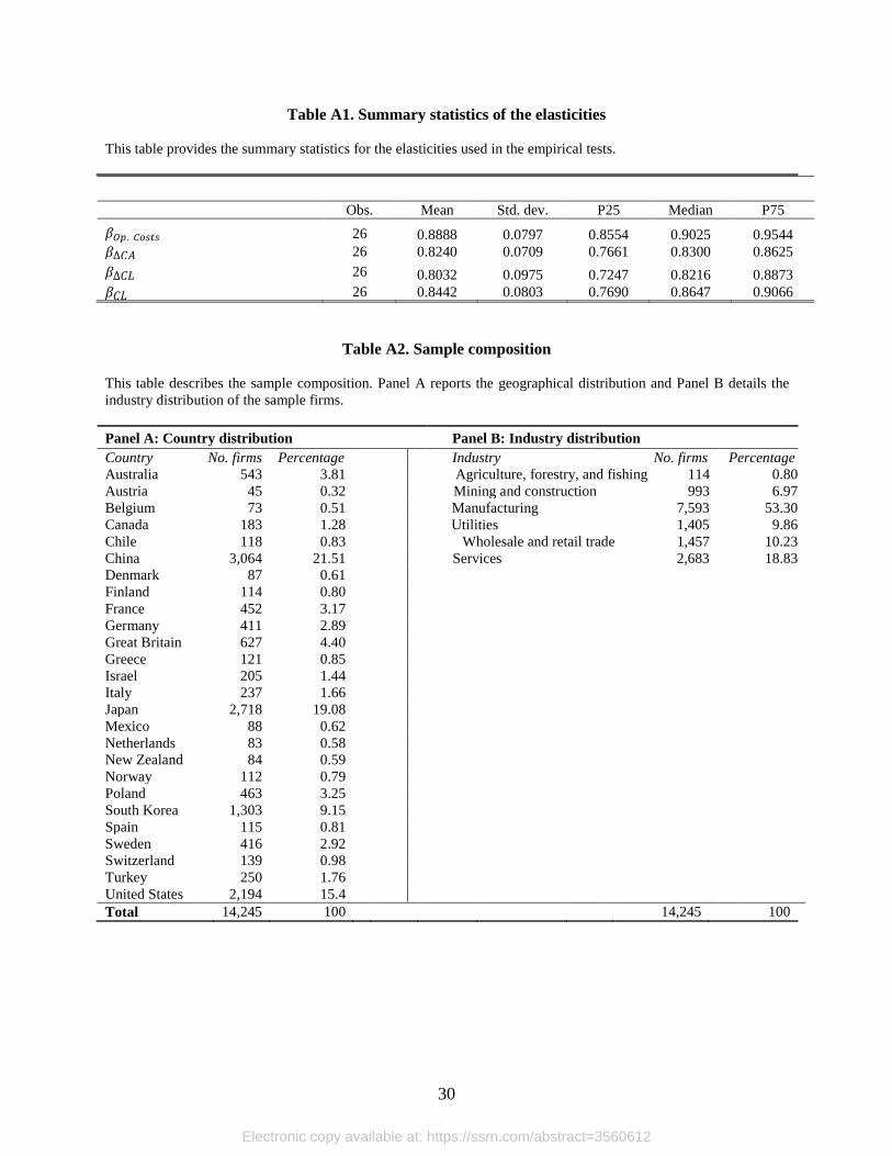
the elasticity of operating costs. The summary statistics of the elasticities are presented in Table A1 of the Internet

Appendix.


9

compute 𝜕𝐶𝐹𝑂 and 𝜕𝐶𝐿 when we assume full operating flexibility, and 𝛽𝑦𝑘 divided by two when

we assume partial operating flexibility.12

3. Data

To examine the liquidity risk of listed firms, we use consolidated firm-level data obtained

from the Compustat Global and North America databases for the fiscal year 2018. We start by

downloading the accounting data for all firms incorporated and headquartered in one of the 35

OECD countries, plus China. To draw meaningful inferences from our analyses, we require each

country to have at least 50 listed firms. This sample requirement excludes 10 of the 35 OECD

member countries. We rely on the International Monetary Fund’s website to retrieve exchange

rates and to convert each variable into US dollars. Furthermore, we collect the corporate tax rates

from the KPMG’s Corporate Tax Guide 2018. We exclude financial firms (SIC codes 6000–

6999) and firms with negative equity, cash holdings, sales, or total assets. These restrictions

result in a sample size of 14,245 unique firms across 26 countries in 2018. Note that all the

analyses focus only on the fiscal year 2018, which is also the last reporting period currently

available. However, for the variables defined in terms of change, such as change in current assets

and change in current liabilities, we also use financial information from the fiscal year 2017.13

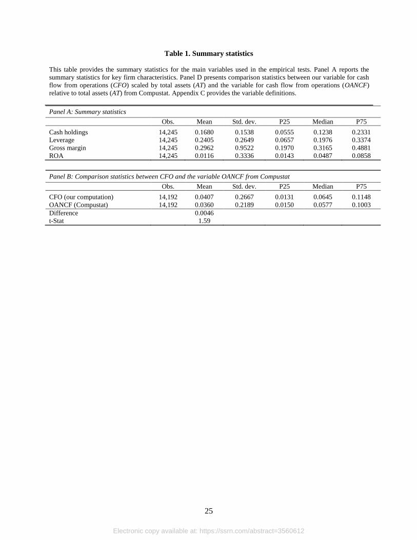
Descriptive statistics for key firm characteristics are presented in Panel A of Table 1. On

average, the sample firms have cash holdings equivalent to 16.8% of their total assets. Further,

the mean value of the gross margin (return on assets, ROA) is 29.62% (1.16%). The average

leverage ratio is about 24.05%.

12 Our methodology is consistent with recent anecdotal evidence, which suggests that several countries have enacted

laws that constrain firms from scaling back production during the outbreak of COVID-19 (e.g., by preventing firms

from laying off employees). For an overview of policy responses to the COVID-19 crisis, see also OECD (2020b).

Moreover, for a similar approach, see Schivardi (2020). 13 Table A2 of the Internet Appendix presents the sample distributions by country (Panel A) and by industry (Panel

B), the latter defined at the one-digit SIC code level.


10

Finally, since we reconstruct the cash flow from operations for each firm in our empirical

analyses, we compare 𝐶𝐹𝑂 to the corresponding cash flow from operations from Compustat

(𝑂𝐴𝑁𝐶𝐹).14 We scale both variables by the total assets in 2018. Panel B of Table 1 presents the

summary statistics and the results of the test for the difference in means of the two variables. As

expected, the variables are not statistically different from each other, suggesting that our variable

closely mirrors that from Compustat.

4. Results

Table 2 presents the base case scenario and the results of the stress tests for the two

simulated distress scenarios. We start by analyzing the cash burn rate. In the base case scenario,

for the average firm in the sample, we find that cash holdings account for about four years and

eight months of annual operating cash flow (column (1) of Panel A).

Next, in Table 2, we focus on the two simulated distress scenarios and allow firms to be

either fully flexible (Panels B to C) or partially flexible (Panels D to E) in their response to the

shock. Starting with firms with full operating flexibility, in column (1) of Panel B we find that

the average firm in the sample would have cash holdings for about two and a half years of annual

operating cash flow in its balance sheet if faced with a moderate-risk scenario (i.e., a drop in

sales of 50%). On the other hand, in the high-risk scenario (column (1) of Panel C), the cash burn

period would last, on average, only two months. However, it is worth pointing out that, in both

scenarios, the distribution of the cash burn rate is negatively skewed. Hence, evaluating the cash

14 Note also that 𝑂𝐴𝑁𝐶𝐹 is missing 53 observations. Since different sample sizes could bias our comparison

analysis, we require both cash flow variables to be nonmissing. This leaves us with 14,192 unique observations.


11

burn rate at the sample median would result in a burn period of about 2-1/2 (1-1/2) years in the

moderate-risk (high-risk) scenario.

With respect to firms with partial operating flexibility, we find that the average cash burn

rate becomes negative in both distress scenarios. In particular, in column (1) of Panel D of Table

2, we find that the average firm in the sample would burn through its cash holdings in about

three years if sales were to drop by 50%. This burn period would further shrink as demand

plummeted, and it would last about two years in the high-risk scenario (column (1) of Panel E).

Figure 1 presents a direct visualization of these tests. We plot the distribution of the cash

burn rate for the base case scenario and the distributions of the cash burn rate for the two

simulated distress scenarios, both under the assumption of full and partial operating flexibility.

Consistent with the previous analyses, we find the distributions of the cash burn rate to be wider

for firms with full operating flexibility, with observations in both the negative and positive tails.

On the other hand, for firms with partial operating flexibility, we observe that the majority of the

observations are concentrated in the negative tail. This finding further suggests that, under partial

operating flexibility, the cash burn rate would become negative for most firms if the demand

were to contract significantly.

What are the implications for the financing of current liabilities? In the base case scenario,

we find that the average firm would be able to cover about 66% of its current liabilities using

cash flow from operations (column (3) of Panel A of Table 2). In the moderate-risk scenario,

when firms are assumed to have operating flexibility, they would still be able to cover a portion,

albeit smaller, of their current liabilities using cash flow from operations. As shown in column

(3) of Panel B in Table 2, the average cash flow from operations would be positive and would


12

amount to about 4 percentage points of current liabilities. On the other hand, in the high-risk

scenario, this ratio would decrease and would become negative (column (3) of Panel C).

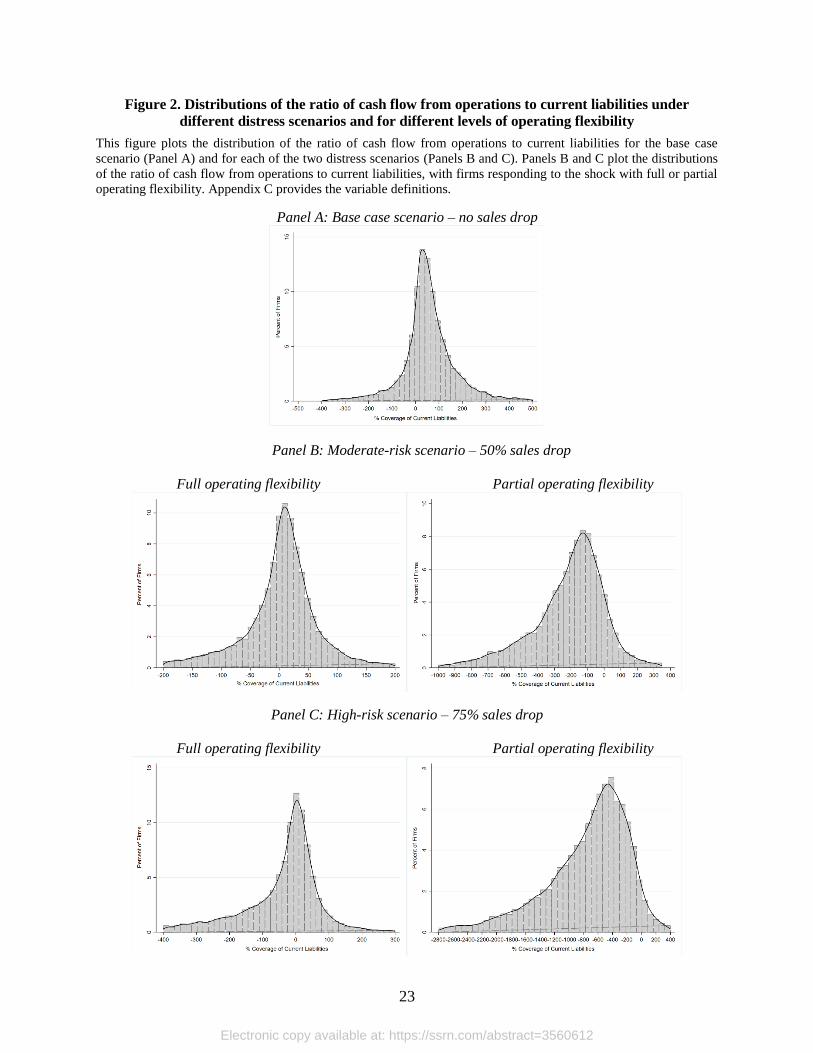
The ratio of cash flow from operations to current liabilities appears to be more problematic

when firms are assumed to have partial flexibility. In both distress scenarios, we find the ratio to

be negative, averaging from −172.76% for the moderate-risk scenario to −779.26% for the high-

risk scenario. This result implies a potential spillover effect that would further magnify the

impact of a sales drop on the cash burn rate of suppliers. Furthermore, in Figure 2, we plot the

distributions of cash flow from operations to current liabilities. Although firms in the base case

scenario and those that are assumed to have full operating flexibility are distributed on both sides

of the density function, we observe that, under the assumption of partial operating flexibility,

firms are mostly concentrated on the negative side of the density function, lending further

support to our previous analyses.

As argued in Section 2.2, to prevent a cash crunch at the end of the burn period, firms with a

negative ratio of cash flow to current liabilities would have to increase the noncurrent liabilities

relative to their level in 2018. As shown in Table 2, firms in the base case scenarios as well as

those in the moderate-risk scenario with full flexibility would not need to issue additional debt,

since their ratio of cash flow from operations to total debt is positive. However, we find that, in

other scenarios, firms would have to increase noncurrent liabilities by about 5.63 (moderate0risk

and fully flexibility scenario) to 53% (high-risk and partial flexibility scenario) in order to avoid

insolvency. These results are also consistent with the distributions of cash flow from operations

to total debt in Figure 3, which are negatively skewed in the high-risk scenario, when firms are

assumed to have full operating flexibility, and in both distress scenarios, when firms are assumed

to have partial operating flexibility.


13

Next, we focus on the most illiquid firms under the assumption of partial operating

flexibility and estimate how many would burn through all their cash holdings in just half a year

in each of the two possible distress scenarios. We operationalize this by computing the number

of firms whose cash burn rate lies between −0.5 and zero. We label these firms as illiquid (i.e.,

firms with high short-term liquidity risk). In column (7) of Table 2, we find that, on average, 717

and 1,367 firms would deplete their cash reserves in half a year in the moderate-risk and high-

risk scenarios, respectively.15

To further analyze the characteristics of these illiquid firms, we conduct two tests, whose

results are shown in Table 3. In Panel A, we present the results of the univariate analysis of key

firm characteristics by differentiating between illiquid and liquid firms. The 1,367 illiquid firms

in the most adverse scenario have a leverage ratio that is, on average, 45% higher than that of the

liquid firms. Further, these illiquid firms have, on average, a negative return on assets, in stark

contrast with the return on assets of the average liquid firm (i.e., about 3.50%). In sum, these

illiquid firms are less profitable, more levered, and hold a lower percentage of cash relative to

total assets compared to their liquid counterparts.16

In Panel B of Table 3, we confirm these results by performing a logistic model whose

dependent variable (Illiquid) is an indicator variable that takes the value of one if the firm is

illiquid, and zero otherwise. We use the firm characteristics from the univariate analysis as

determinants of short-term liquidity risk. Furthermore, we include industry fixed effects to

absorb industry shocks that could affect the probability of a firm becoming illiquid. We include

15 Table A3 of the Internet Appendix presents the distribution of illiquid firms with partial operating flexibility by

country for the base case scenario and for each of the two distress scenarios. 16 In untabulated results of univariate analyses, we continue to find that, in the moderate-risk scenario, the most

illiquid firms are, on average, less profitable and more levered than their liquid counterparts are. The results are

available upon request.


14

country fixed effects to ensure that unobservable political and economic conditions do not

spuriously drive the results.

In line with the univariate analysis, in column (1) of Panel B of Table 3, we find that the

likelihood of becoming illiquid within six months is significantly higher when a firm has a

higher leverage ratio, whereas it is significantly lower when a firm has more cash holdings

relative to total assets, a higher gross margin, and a higher return on assets. In terms of economic

significance, a one-standard-deviation increase in the leverage ratio is associated with a 0.57% (=

2.16% × 0.2649) increase in the probability of becoming illiquid within six months. Relatedly, a

one-standard-deviation increase in the cash holdings, gross margin, and return on assets is

associated with a 7.11%, 0.31%, and 2.79% decrease, respectively, in the probability of

becoming illiquid. Importantly, in column (2) of Panel B, we find that the results hold when

country–industry fixed effects are included to account for any country–industry-specific factor

that could affect the probability of becoming illiquid (e.g., different exposures and durations of

exposure of countries and industries to COVID-19).

5. Policy implications

In the last set of analyses, we examine the policy implications of our results. Specifically,

we investigate which fiscal measures could be more effective in ameliorating the risk of a

COVID-19 cash crunch. Focusing on firms assumed to have partial operating flexibility in the

moderate- and high-risk scenarios, we analyze two policies: a six-month tax deferral and a direct

provision of cash to firms as a lump sum akin to a bridge loan granted by the government.

Although both measures mitigate short-term liquidity risk, they work in different directions. In

particular, the tax deferral decreases a firm’s current taxes, whereas the bridge loan increases a


15

firm’s cash holdings.17 To operationalize this, for each illiquid firm in both distress scenarios, we

increase either the denominator of the cash burn rate for the amount of a six-month tax deferral

or the numerator for the amount of a bridge loan that would adjust the cash burn rate to −0.5.

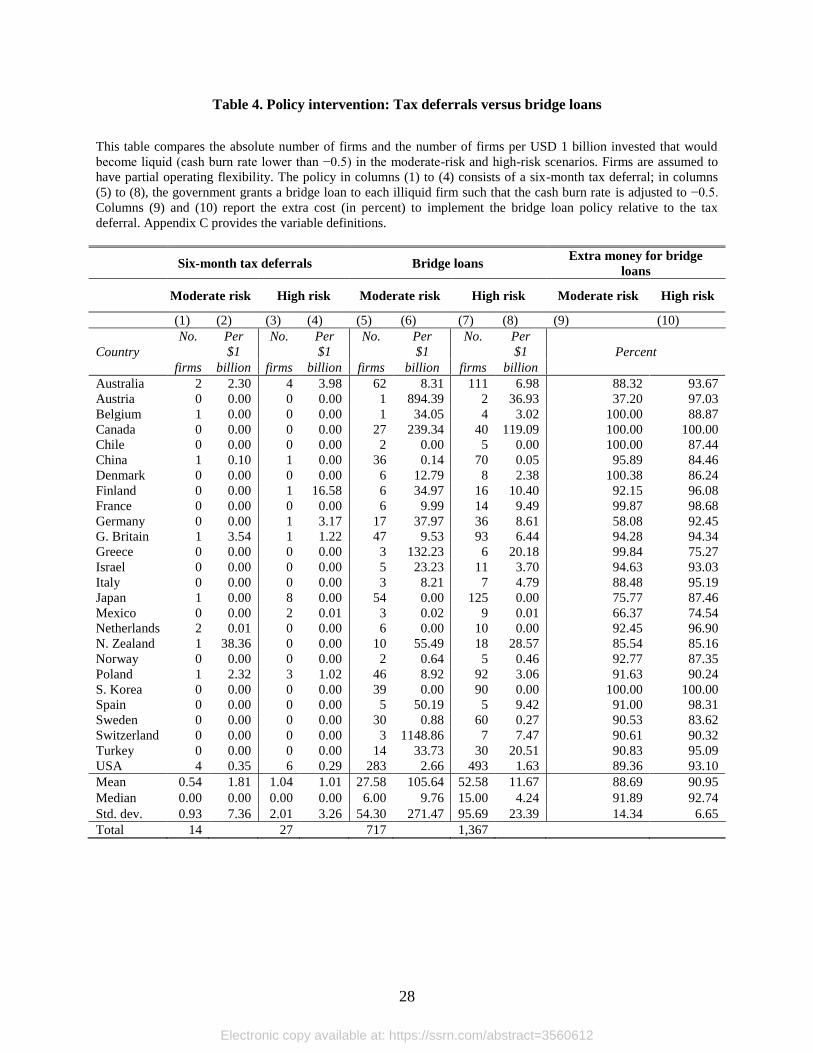
Table 4 presents the results. Columns (1) and (3) show the number of firms that a two-

quarter tax deferral would prevent from becoming illiquid within six months. In total, a half-a-

year tax deferral would prevent only 14 (27) firms from becoming illiquid within six months in

the moderate-risk (high-risk) scenario. On the other hand, columns (5) and (7) assume that the

government facilitates a bridge loan to the 717 (1,367) illiquid firms in the moderate-risk (high-

risk) scenario to shore up all their cash burn rates to −0.5. With respect to the costs of each

measure, columns (9) and (10) show that the bridge loan is, on average, twice as costly as a six-

month tax deferral. Nevertheless, the bridge loan appears to be more cost-effective than a tax

deferral. As shown in columns (2) and (4), on average, 1.8 (one) firms would avoid a cash

crunch within six months per USD 1 billion of deferred taxes in the moderate-risk (high-risk)

scenario. On the other hand, columns (6) and (8) show that a bridge loan to each firm for the

amount necessary to prevent a cash crunch within six months would, on average, save 105.64

(11.67) firms per USD 1 billion loan from becoming illiquid within six months in the moderate-

risk (high-risk) scenario.

6. Conclusion

In this paper, we examine how the COVID-19 health crisis could affect the liquidity risk of

listed firms. To this end, we first collect detailed data on 14,245 listed firms across 26 countries

and compute three financial ratios that are widely used in the accounting literature to assess

short-term and long-term liquidity risk. Subsequently, we stress-test the three liquidity ratios in

17 Appendix B shows analytically that, when a firm has a cash burn rate between zero and -1 year, a dollar invested

in a cash transfer decreases the cash burn rate (i.e., increases the firm’s liquidity) more than a dollar invested in

increasing the operating cash flow via tax deferrals.


16

two simulated distress scenarios, corresponding to drops in sales of 50% and 75%, respectively.

We assume that firms either have full or partial operating flexibility. In the most adverse

scenario, and under the assumption of partial operating flexibility, we find that the average firm

would exhaust its cash holdings in about two years. At that point, its current liabilities would

increase beyond a sustainable level, such that an injection of about 53% of noncurrent debt

(relative to the 2018 level) would be needed to prevent a liquidity crunch. Moreover, about

1/10th of all firms would become illiquid within six months.

Finally, we study two different fiscal policies, namely, tax deferrals and bridge loans, that

governments could implement to mitigate the risk of a COVID-19 cash crunch. Our analyses

suggest that bridge loans are more cost-effective in preventing a massive cash crunch within six

months after the shock. Whether the COVID-19 cash crunch is larger and more pressing for

unlisted firms is a question we leave for future research.


17

References

Adda, J., 2016. Economic activity and the spread of viral diseases: Evidence from high frequency

data. Quarterly Journal of Economics, 131, 891-941.

Baldwin, R., Weder di Mauro, B., 2020. Mitigating the COVID Economic Crisis: Act Fast and

Do Whatever It Takes. CEPR Press.

Banker, R. D., Byzalov, D., Chen, L. T., 2013. Employment protection legislation, adjustment

costs, and cross-country differences in cost behavior. Journal of Accounting and

Economics, 55, 111-127.

Becker, B., Ivashina, V., 2014. Cyclicality of credit supply: Firm level evidence, Journal of

Monetary Economics, 62, 76-93.

Bénassy-Quéré, A., Marimon, R., Pisani-Ferry, J., Reichlin, L., Schoenmaker, D., Weder di

Mauro B., 2020. Europe Needs a Catastrophe Relief Plan. CEPR Press, London.

Bischof, J., Daske, H., 2013. Mandatory disclosure, voluntary disclosure, and stock market

liquidity: Evidence from the EU bank stress tests. Journal of Accounting Research, 51(5),

997-1029.

Bloom, D. E., Cadarette, D., Sevilla J. P., 2018. Epidemics and economics. Finance &

Development, 55, 46-49.

Bowen, R. M., Davis, A. K., Rajgopal, S., 2002. Determinants of revenue-reporting practices for

internet firms. Contemporary Accounting Research, 19(4), 523-562.

De Haas, R., Van Horen, N., 2013. Running for the exit? International bank lending during a

financial crisis. Review of Financial Studies, 26, 244–285.

Fan, V., Jamison, D. T., Summers, L. H., 2018. Pandemic risk: How large are the expected

losses? Bulletin World Health Organization, 96(2), 129-134.

Fornaro, L., Wolf, M., 2020. COVID-19 coronavirus and macroeconomic policy: Some

analytical notes. SSRN working paper.

Huizinga, H., Laeven, L., 2012. Bank valuation and accounting discretion during a financial

crisis. Journal of Financial Economics, 106(3), 614-634.

McKibbin, W., Fernando, R., 2020. The global macroeconomic impacts of COVID-19: Seven

scenarios. Centre for Applied Macroeconomic Analysis working paper No. 19/2020.

OECD, 2020a. OECD Economic Outlook - Interim Report March 2020. OECD Publishing, Paris.

OECD, 2020b. Supporting People and Companies to Deal with the COVID-19 Virus: Options for

an Immediate Employment and Social-Policy Response. OECD Publishing Paris.


18

Petrella, G., Resti, A., 2013. Supervisors as information producers: Do stress tests reduce bank

opaqueness? Journal of Banking and Finance, 37(12), 5406-5420.

Ramelli, S., Wagner, A., 2020. Feverish stock price reactions to COVID-19. SSRN working

paper.

Schivardi, F., 2020. Come evitare il contagio finanziario alle imprese. Lavoce.info, March 24,

2020.


19

Appendix A. Theoretical derivation of Eq. (1)

In this appendix, we model how a given percentage drop in sales affects a firm’s cash flow from

operations. Let us define net income 𝑁𝐼 as

𝑁𝐼 = 𝑆𝑎𝑙𝑒𝑠 − 𝑂𝑝. 𝐶𝑜𝑠𝑡𝑠 − 𝐷𝑒𝑝𝑟 − 𝐼𝑛𝑡𝑒𝑟𝑒𝑠𝑡𝑠 − 𝐶𝑢𝑟𝑟𝑒𝑛𝑡 𝑇𝑎𝑥𝑒𝑠 (A.1)

where 𝑆𝑎𝑙𝑒𝑠 denotes sales, 𝑂𝑝. 𝐶𝑜𝑠𝑡𝑠 denotes operating expenses, 𝐷𝑒𝑝𝑟 stands for depreciation and

amortization, 𝐼𝑛𝑡𝑒𝑟𝑒𝑠𝑡𝑠 denotes interest payments on debt, and 𝐶𝑢𝑟𝑟𝑒𝑛𝑡 𝑇𝑎𝑥𝑒𝑠 denotes current taxes. To

estimate funds from operations (𝐹𝐹𝑂), 𝐷𝑒𝑝𝑟 and 𝐷𝑒𝑓𝑒𝑟𝑟𝑒𝑑 𝑇𝑎𝑥𝑒𝑠 to 𝑁𝐼 are added back, as follows:

𝐹𝐹𝑂 = 𝑁𝐼 + 𝐷𝑒𝑝𝑟 + 𝐷𝑒𝑓𝑒𝑟𝑟𝑒𝑑 𝑇𝑎𝑥𝑒𝑠 (A.2)

To arrive at cash flow from operations (𝐶𝐹𝑂), we subtract the change in current assets (𝛥𝐶𝐴), net of cash

holdings, and add change in current liabilities (𝛥𝐶𝐿), as follows:

𝐶𝐹𝑂 = 𝐹𝐹𝑂 − 𝛥𝐶𝐴 + 𝛥𝐶𝐿 (A.3)

Given Eqs. (A.1) to (A.3), the change in cash flow from operations with respect to sales is

𝜕𝐶𝐹𝑂

𝜕𝑆𝑎𝑙𝑒𝑠= 1 −

𝜕𝑂𝑝.𝐶𝑜𝑠𝑡𝑠

𝜕𝑆𝑎𝑙𝑒𝑠−

𝜕𝐶𝑢𝑟𝑟𝑒𝑛𝑡 𝑇𝑎𝑥𝑒𝑠

𝜕𝑆𝑎𝑙𝑒𝑠−

𝜕∆𝐶𝐴

𝜕𝑆𝑎𝑙𝑒𝑠+

𝜕∆𝐶𝐿

𝜕𝑆𝑎𝑙𝑒𝑠 (A.4)

where we assume that, in the short run, interest payments and deferred taxes are invariant with respect to

sales; that is, a firm neither changes its capital structure nor renegotiates its debt. By multiplying both

sides of (A.4) by 𝑆𝑎𝑙𝑒𝑠, we can express (A.4) as

𝜕𝐶𝐹𝑂𝜕𝑆𝑎𝑙𝑒𝑠

𝑆𝑎𝑙𝑒𝑠

= 𝑆𝑎𝑙𝑒𝑠 − 𝑂𝑝. 𝐶𝑜𝑠𝑡𝑠 × 𝐸𝑂𝑝. 𝐶𝑜𝑠𝑡𝑠 − 𝐶𝑢𝑟𝑟𝑒𝑛𝑡 𝑇𝑎𝑥𝑒𝑠 × 𝐸𝐶𝑢𝑟𝑟𝑒𝑛𝑡 𝑇𝑎𝑥𝑒𝑠 − ∆𝐶𝐴 × 𝐸∆𝐶𝐴 + ∆𝐶𝐿 × 𝐸∆𝐶𝐿 (A.5)

where 𝐸𝑋 =𝜕𝑋/𝑋

𝜕𝑆𝑎𝑙𝑒𝑠/𝑆𝑎𝑙𝑒𝑠 denotes the elasticity of X with respect to sales, with 𝑋 =

{𝑂𝑝. 𝐶𝑜𝑠𝑡𝑠, 𝐶𝑢𝑟𝑟𝑒𝑛𝑡 𝑇𝑎𝑥𝑒𝑠, ∆𝐶𝐴, ∆𝐶𝐿}. In other words, 𝐸𝑋 corresponds to the percentage change in each

of these variables with respect to a 1% change in sales. The right-hand side of (A.5) can be interpreted as

the dollar change in cash flows from operations for a 1% change in sales.

We define current taxes as

𝐶𝑢𝑟𝑟𝑒𝑛𝑡 𝑇𝑎𝑥𝑒𝑠 = (𝑆𝑎𝑙𝑒𝑠 − 𝑂𝑝. 𝐶𝑜𝑠𝑡𝑠 − 𝐷𝑒𝑝𝑟 − 𝐼𝑛𝑡𝑒𝑟𝑒𝑠𝑡𝑠) × 𝑇𝑅 (A.6)

where 𝑇𝑅 is the statutory corporate tax rate. We assume that 𝐷𝑒𝑝𝑟 and 𝐼𝑛𝑡𝑒𝑟𝑒𝑠𝑡𝑠 are invariant with

respect to sales in the short run. By taking the derivative of (A.6) with respect to sales and multiplying it

by 𝑆𝑎𝑙𝑒𝑠 over 𝐶𝑢𝑟𝑟𝑒𝑛𝑡 𝑇𝑎𝑥𝑒𝑠, we obtain the elasticity of current taxes with respect to sales as follows:

𝐸𝐶𝑢𝑟𝑟𝑒𝑛𝑡 𝑇𝑎𝑥𝑒𝑠 =𝜕𝐶𝑢𝑟𝑟𝑒𝑛𝑡 𝑇𝑎𝑥𝑒𝑠/𝐶𝑢𝑟𝑟𝑒𝑛𝑡 𝑇𝑎𝑥𝑒𝑠

𝜕𝑆𝑎𝑙𝑒𝑠

𝑆𝑎𝑙𝑒𝑠

= (𝑆𝑎𝑙𝑒𝑠 − 𝑂𝑝. 𝐶𝑜𝑠𝑡𝑠 × 𝐸𝑂𝑝. 𝐶𝑜𝑠𝑡𝑠) ×𝑇𝑅

𝐶𝑢𝑟𝑟𝑒𝑛𝑡 𝑇𝑎𝑥𝑒𝑠 (A.7)

By replacing (A.7) into (A.5), we obtain Eq. (1) of the paper, which corresponds to the change in the

dollar amount of cash flow from operations with respect to a 𝜕𝑆𝐴𝐿𝐸

𝑆𝐴𝐿𝐸 percent change in sales.


20

Appendix B. Theoretical discussion of the benefit of bridge loans versus tax deferrals

In line with our theoretical framework, after a drop in sales, the cash burn rate is defined as follows:

𝐶𝑎𝑠ℎ 𝑏𝑢𝑟𝑛 𝑟𝑎𝑡𝑒 =𝐶𝑎𝑠ℎ


where 𝐶𝑎𝑠ℎ and 𝐶𝐹𝑂 denote cash holdings plus accounts receivable and annual cash flow from

operations, respectively, and 𝜕𝐶𝐹𝑂 denotes the change in 𝐶𝐹𝑂, as in Eq. (1). Let us now assume that,

after a decrease in sales, 𝐶𝐹𝑂 + 𝜕𝐶𝐹𝑂 < 0, such that the cash burn rate corresponds to the number of

years before the firm becomes illiquid. Marginally, for every dollar increase in the value of 𝐶𝑎𝑠ℎ for the

firm, the cash burn ratio decreases by

𝜕

𝜕 𝐶𝑎𝑠ℎ𝐶𝐵 =

1


Similarly, for every dollar increase in the firm’s cash flow from operations (𝐶𝐹𝑂), the cash burn rate

decreases by

𝜕

𝜕 𝐶𝐹𝑂𝐶𝐵 = −

𝐶𝑎𝑠ℎ

(𝐶𝐹𝑂 + 𝜕𝐶𝐹𝑂)2

Then, it follows immediately that

𝜕

𝜕 𝐶𝑎𝑠ℎ𝐶𝐵 <

𝜕

𝜕 𝐶𝐹𝑂𝐶𝐵 𝑖𝑓 𝑎𝑛𝑑 𝑜𝑛𝑙𝑦 𝑖𝑓 − 1 < 𝐶𝐵 < 0

Hence, at the margin, one extra dollar in cash extends the time to illiquidity more than one dollar in tax

deferrals (or any other cost reduction measure) if and only if the firm currently has less than one year

before it becomes illiquid.


21

Appendix C. Variable definitions

Variable Definition

CFO Sales (𝑆𝐴𝐿𝐸) minus operating costs (𝑋𝑂𝑃𝑅), current taxes (𝑇𝑋𝐶), interest

payments (𝑋𝐼𝑁𝑇), and change in current assets net of cash holdings

(∆𝐴𝐶𝑇 − 𝐶𝐻𝐸), plus deferred taxes (𝑇𝑋𝐷𝐼) and change in current liabilities

(∆𝐿𝐶𝑇). (Source: Compustat)

∂CFO ((𝑆𝐴𝐿𝐸 − (𝑋𝑂𝑃𝑅 × 1

2𝐸𝑋𝑂𝑃𝑅)) × (1× 𝑇𝑎𝑥 𝑅𝑎𝑡𝑒)) – (∆(𝐴𝐶𝑇 − 𝐶𝐻𝐸) ×

1

2𝐸∆(𝐴𝐶𝑇−𝐶𝐻𝐸)) + (∆𝐿𝐶𝑇 ×

1

2𝐸∆𝐿𝐶𝑇). We compute each elasticity 𝐸𝑋 by

estimating country-level regressions with industry (one-digit SIC code) and

year fixed effects of the natural logarithm of a firm’s sales (𝑆𝐴𝐿𝐸) on each

of the following variables: the natural logarithm of a firm’s operating costs

(𝑋𝑂𝑃𝑅), the natural logarithm of change in current assets net of cash

holdings (∆𝐴𝐶𝑇 − 𝐶𝐻𝐸), and the natural logarithm of change in current

liabilities (∆𝐿𝐶𝑇). (Source: Compustat and KPMG Corporate Tax Guide

2018)

Cash burn rate Cash and short-term investments (CHE) plus accounts receivable (RECT)

relative to the sum of the cash flow from operations and the change in cash

flow from operations (𝐶𝐹𝑂 + 𝜕𝐶𝐹𝑂). (Source: Compustat)

Cash flow from operations (CFO) to current liabilities

The sum of cash flow from operations and the change in cash flow from

operations (𝐶𝐹𝑂 + 𝜕𝐶𝐹𝑂) relative to the sum of current liabilities and the

change in current liabilities ((𝐿𝐶𝑇 ×1

2𝐸𝐿𝐶𝑇) + ((𝐿𝐶𝑇 ×

1

2𝐸𝐶𝐿) ×

% 𝑑𝑟𝑜𝑝 𝑖𝑛 𝑠𝑎𝑙𝑒𝑠). We compute 𝐸𝐶𝐿 by estimating country-level regressions

with industry (one-digit SIC code) and year fixed effects of the natural

logarithm of a firm’s sales (𝑆𝐴𝐿𝐸) on the natural logarithm of current

liabilities (LCT). The drop in sales takes on the value of 50 (75) in the

moderate-risk (high-risk) scenario. (Source: Compustat)

Cash flow from operations

(CFO) to total debt

The sum of cash flow from operations and the change in cash flow from

operations (𝐶𝐹𝑂 + 𝜕𝐶𝐹𝑂) relative to total liabilities (𝐿𝑇). (Source:

Compustat)

Illiquid Indicator variable that takes the value of 1 if the firm’s cash burn rate lies

between −0.5 and 0, and zero otherwise. (Source: Compustat)

Cash holdings Cash and short-term investments (CHE) scaled by total assets (AT).

(Source: Compustat)

Leverage Total debt (DLC + DLTT) relative to total assets (AT). (Source: Compustat)

Gross margin Sales (SALE) minus the cost of goods sold (COGS) relative to sales (SALE).

(Source: Compustat)

ROA Earnings before interests and taxes (EBIT) scaled by total assets (AT).

(Source: Compustat)

Tax deferral Current taxes (TXC) times 0.50. The cash burn rate with a six-month tax

deferral is defined as cash and short-term investments (CHE) plus accounts

receivable (RECT) relative to the sum of the cash flow from operations, the

change in cash flow from operations, and the tax deferral (𝐶𝐹𝑂 + 𝜕𝐶𝐹𝑂 +(𝑇𝑋𝐶 × 0.50)). (Source: Compustat)

Bridge loans −1 times the sum of the cash flow from operations and the change in cash

flow from operations (𝐶𝐹𝑂 + 𝜕𝐶𝐹𝑂) times the sum of the cash burn rate of

the distress scenario considered and 0.5. (Source: Compustat)

Extra money for bridge loan The total amount of the country’s bridge loans minus the total amount of

the country’s tax deferral relative to the total amount of its bridge loans,

times 100. (Source: Compustat)


22

Figure 1. Distributions of the cash burn rate under different distress scenarios and for different

levels of operating flexibility

This figure plots the distribution of the cash burn rate for the base case scenario (Panel A) and for each of the two

distress scenarios (Panels B and C). Panels B and C plot the distributions of the cash burn rate allowing firms to

respond to the shock with full or partial operating flexibility. Appendix C provides the variable definitions.

Panel A: Base case scenario – no sales drop

Panel B: Moderate-risk scenario – 50% sales drop

Full operating flexibility Partial operating flexibility

Panel C: High-risk scenario – 75% sales drop



23

Figure 2. Distributions of the ratio of cash flow from operations to current liabilities under

different distress scenarios and for different levels of operating flexibility

This figure plots the distribution of the ratio of cash flow from operations to current liabilities for the base case

scenario (Panel A) and for each of the two distress scenarios (Panels B and C). Panels B and C plot the distributions

of the ratio of cash flow from operations to current liabilities, with firms responding to the shock with full or partial

operating flexibility. Appendix C provides the variable definitions.







24

Figure 3. Distributions of the ratio of cash flow from operations to total debt under different

distress scenarios and for different levels of operating flexibility

This figure plots the distributions of the ratio of cash flow from operations to total debt (for 2018) for the base case

scenario (Panel A) and for each of the two distress scenarios (Panels B and C). Panels B and C plot the distributions

of the ratio of cash flow from operations to total debt, with firms responding to the shock with full or partial

operating flexibility. Appendix C provides the variable definitions.







25

Table 1. Summary statistics

This table provides the summary statistics for the main variables used in the empirical tests. Panel A reports the

summary statistics for key firm characteristics. Panel D presents comparison statistics between our variable for cash

flow from operations (CFO) scaled by total assets (AT) and the variable for cash flow from operations (OANCF)

relative to total assets (AT) from Compustat. Appendix C provides the variable definitions.

Panel A: Summary statistics

Obs. Mean Std. dev. P25 Median P75

Cash holdings 14,245 0.1680 0.1538 0.0555 0.1238 0.2331

Leverage 14,245 0.2405 0.2649 0.0657 0.1976 0.3374

Gross margin 14,245 0.2962 0.9522 0.1970 0.3165 0.4881

ROA 14,245 0.0116 0.3336 0.0143 0.0487 0.0858

Panel B: Comparison statistics between CFO and the variable OANCF from Compustat


CFO (our computation) 14,192 0.0407 0.2667 0.0131 0.0645 0.1148

OANCF (Compustat) 14,192 0.0360 0.2189 0.0150 0.0577 0.1003

Difference 0.0046

t-Stat 1.59


26

Table 2. Stress tests of the cash burn rate, the ratio of cash flow from operations to current

liabilities, and the ratio of cash flow from operations to total debt under different distress scenarios

and for different levels of operating flexibility

This table presents the base case scenario (Panel A) and the results of the stress tests for the moderate-risk scenario

(Panels B and D) and the high-risk scenario (Panels C and E) for different levels of operating flexibility. Appendix C

provides the variable definitions.


Cash burn rate (years) CFO to current liab. (%) CFO to total debt (%) Illiquid firms

(1) (2) (3) (4) (5) (6) (7) (8)

Mean Median Mean Median Mean Median Number Percentage

4.71 2.68 66.00 49.00 15.41 12.94 226 1.59

Full operating flexibility



(1) (2) (3) (4) (5) (6) (7) (8)


2.41 2.66 4.65 8.79 1.32 2.37 228 1.60



(1) (2) (3) (4) (5) (6) (7) (8)


−0.19 −1.61 −52.20 −12.79 −5.63 −1.85 287 2.01

Partial operating flexibility

Panel D: Moderate-risk scenario – 50% sales drop


(1) (2) (3) (4) (5) (6) (7) (8)


−2.98 −2.10 −216.01 −172.76 −30.27 −24.18 717 5.03

Panel E: High-risk scenario – 75% sales drop


(1) (2) (3) (4) (5) (6) (7) (8)


−2.15 −1.48 −779.26 −620.40 −53.05 −42.94 1,367 9.60


27

Table 3. Differences between illiquid and liquid firms with partial operating flexibility in the high-

risk scenario

This table examines the difference between illiquid and liquid firms with partial operating flexibility in the high-risk

scenario. Panel A provides the results of univariate analysis, whereas Panel B provides the results of logistic

regression examining the determinants of a firm’s illiquidity. In Panel B, columns (1) and (3) present the coefficient

estimates, whereas columns (2) and (4) present the marginal effects at the means. The model specifications

presented in columns (1) and (3) include industry, country, and country–industry fixed effects where indicated. The

industry is defined at the one-digit SIC code level. The table reports (in parentheses) heteroskedasticity-robust

standard errors. ***, **, and * denote statistical significance at the 1%, 5%, and 10% levels (two tailed),

respectively. Appendix C provides the variable definitions.

Panel A: Difference in means

Illiquid firms Liquid firms Difference t-Stat

(1) (2) (3) (4)

Cash holdings 0.0725 0.1781 −0.1056*** −33.2849

Leverage 0.4134 0.2221 0.1913*** 14.5758

Gross margin 0.0479 0.3226 −0.2747*** −5.2879

ROA −0.2075 0.0350 −0.1725*** −10.2996

Panel B: Determinants of illiquidity

Illiquid

(1) (2) (3) (4)

Coefficient Marginal effect Coefficient Marginal effect

Cash holdings −10.2752*** −46.23% −10.0394*** −46.13%

(0.6323) (0.6301)

Leverage 0.4790*** 2.16% 0.4874*** 2.24%

(0.1449) (0.1449)

Gross margin −0.0727** −0.33% −0.0577 −0.27%

(0.0361) (0.0363)

ROA −1.8600*** −8.37% −1.8598*** −8.55%

(0.2372) (0.2332)

Constant −2.4898*** −2.0416***

(0.1319) (0.1209)

Industry fixed effects Yes No

Country fixed effects Yes No

Country−Industry fixed effects No Yes

Obs. 14,245 14,245

Pseudo-R2 0.189 0.182


28

Table 4. Policy intervention: Tax deferrals versus bridge loans

This table compares the absolute number of firms and the number of firms per USD 1 billion invested that would

become liquid (cash burn rate lower than −0.5) in the moderate-risk and high-risk scenarios. Firms are assumed to

have partial operating flexibility. The policy in columns (1) to (4) consists of a six-month tax deferral; in columns

(5) to (8), the government grants a bridge loan to each illiquid firm such that the cash burn rate is adjusted to −0.5.

Columns (9) and (10) report the extra cost (in percent) to implement the bridge loan policy relative to the tax

deferral. Appendix C provides the variable definitions.

Six-month tax deferrals Bridge loans Extra money for bridge

loans

Moderate risk High risk Moderate risk High risk Moderate risk High risk

(1) (2) (3) (4) (5) (6) (7) (8) (9) (10)

Country

No. Per

$1

No. Per

$1

No. Per

$1

No. Per

$1 Percent

firms billion firms billion firms billion firms billion

Australia 2 2.30 4 3.98 62 8.31 111 6.98 88.32 93.67

Austria 0 0.00 0 0.00 1 894.39 2 36.93 37.20 97.03

Belgium 1 0.00 0 0.00 1 34.05 4 3.02 100.00 88.87

Canada 0 0.00 0 0.00 27 239.34 40 119.09 100.00 100.00

Chile 0 0.00 0 0.00 2 0.00 5 0.00 100.00 87.44

China 1 0.10 1 0.00 36 0.14 70 0.05 95.89 84.46

Denmark 0 0.00 0 0.00 6 12.79 8 2.38 100.38 86.24

Finland 0 0.00 1 16.58 6 34.97 16 10.40 92.15 96.08

France 0 0.00 0 0.00 6 9.99 14 9.49 99.87 98.68

Germany 0 0.00 1 3.17 17 37.97 36 8.61 58.08 92.45

G. Britain 1 3.54 1 1.22 47 9.53 93 6.44 94.28 94.34

Greece 0 0.00 0 0.00 3 132.23 6 20.18 99.84 75.27

Israel 0 0.00 0 0.00 5 23.23 11 3.70 94.63 93.03

Italy 0 0.00 0 0.00 3 8.21 7 4.79 88.48 95.19

Japan 1 0.00 8 0.00 54 0.00 125 0.00 75.77 87.46

Mexico 0 0.00 2 0.01 3 0.02 9 0.01 66.37 74.54

Netherlands 2 0.01 0 0.00 6 0.00 10 0.00 92.45 96.90

N. Zealand 1 38.36 0 0.00 10 55.49 18 28.57 85.54 85.16

Norway 0 0.00 0 0.00 2 0.64 5 0.46 92.77 87.35

Poland 1 2.32 3 1.02 46 8.92 92 3.06 91.63 90.24

S. Korea 0 0.00 0 0.00 39 0.00 90 0.00 100.00 100.00

Spain 0 0.00 0 0.00 5 50.19 5 9.42 91.00 98.31

Sweden 0 0.00 0 0.00 30 0.88 60 0.27 90.53 83.62

Switzerland 0 0.00 0 0.00 3 1148.86 7 7.47 90.61 90.32

Turkey 0 0.00 0 0.00 14 33.73 30 20.51 90.83 95.09

USA 4 0.35 6 0.29 283 2.66 493 1.63 89.36 93.10

Mean 0.54 1.81 1.04 1.01 27.58 105.64 52.58 11.67 88.69 90.95

Median 0.00 0.00 0.00 0.00 6.00 9.76 15.00 4.24 91.89 92.74

Std. dev. 0.93 7.36 2.01 3.26 54.30 271.47 95.69 23.39 14.34 6.65

Total 14 27 717 1,367


29

Estimating the COVID-19 Cash Crunch: Global Evidence and

Policy

Antonio De Vito

Juan-Pedro Gómez

Internet Appendix


30

Table A1. Summary statistics of the elasticities

This table provides the summary statistics for the elasticities used in the empirical tests.


𝛽𝑂𝑝. 𝐶𝑜𝑠𝑡𝑠 26 0.8888 0.0797 0.8554 0.9025 0.9544

𝛽∆𝐶𝐴 26 0.8240 0.0709 0.7661 0.8300 0.8625

𝛽∆𝐶𝐿 26 0.8032 0.0975 0.7247 0.8216 0.8873

𝛽𝐶𝐿 26 0.8442 0.0803 0.7690 0.8647 0.9066

Table A2. Sample composition

This table describes the sample composition. Panel A reports the geographical distribution and Panel B details the

industry distribution of the sample firms.

Panel A: Country distribution Panel B: Industry distribution

Country No. firms Percentage Industry No. firms Percentage

Australia 543 3.81 Agriculture, forestry, and fishing 114 0.80

Austria 45 0.32 Mining and construction 993 6.97

Belgium 73 0.51 Manufacturing 7,593 53.30

Canada 183 1.28 Utilities 1,405 9.86

Chile 118 0.83 Wholesale and retail trade 1,457 10.23

China 3,064 21.51 Services 2,683 18.83

Denmark 87 0.61

Finland 114 0.80

France 452 3.17

Germany 411 2.89

Great Britain 627 4.40

Greece 121 0.85

Israel 205 1.44

Italy 237 1.66

Japan 2,718 19.08

Mexico 88 0.62

Netherlands 83 0.58

New Zealand 84 0.59

Norway 112 0.79

Poland 463 3.25

South Korea 1,303 9.15

Spain 115 0.81

Sweden 416 2.92

Switzerland 139 0.98

Turkey 250 1.76

United States 2,194 15.4

Total 14,245 100 14,245 100


31

Table A3. Distributions of illiquid firms with partial operating flexibility under different distress

scenarios

This table reports the numbers and percentages of firms, relative to the total in each given country, for which Illiquid

is equal to one in the base case scenario (columns (1) and (2)). It also reports the numbers and percentages of firms,

relative to the total in each given country, with partial operating flexibility for which Illiquid takes the value of one

for each of the two simulated distress scenarios (columns (3) to (6)). Appendix C provides the variable definitions.

Base case Moderate risk High risk

(1) (2) (3) (4) (5) (6)

Country No. firms % firms No. firms % firms No. firms % firms

Australia 29 5.34 62 11.42 111 20.44

Austria 0 0.00 1 2.22 2 4.44

Belgium 0 0.00 1 1.37 4 5.48

Canada 15 8.20 27 14.75 40 21.86

Chile 0 0.00 2 1.69 5 4.24

China 13 0.42 36 1.17 70 2.28

Denmark 3 3.45 6 6.90 8 9.20

Finland 1 0.88 6 5.26 16 14.04

France 4 0.88 6 1.33 14 3.10

Germany 5 1.22 17 4.14 37 9.00

Great Britain 8 1.28 47 7.50 93 14.83

Greece 2 1.65 3 2.48 6 4.96

Israel 4 1.95 5 2.44 11 5.37

Italy 1 0.42 3 1.27 7 2.95

Japan 2 0.07 54 1.99 125 4.60

Mexico 0 0.00 3 3.41 9 10.23

Netherlands 0 0.00 6 7.23 10 12.05

New Zealand 3 3.57 10 11.90 18 21.43

Norway 0 0.00 2 1.79 4 3.57

Poland 12 2.59 46 9.94 92 19.87

South Korea 14 1.07 39 2.99 90 6.91

Spain 2 1.74 5 4.35 5 4.35

Sweden 13 3.13 30 7.21 60 14.42

Switzerland 1 0.72 3 2.16 7 5.04

Turkey 5 2.00 14 5.60 30 12.00

United States 89 4.06 283 12.90 493 22.47

Mean 11.30 2.23 27.58 5.21 52.58 9.97

Median 4.50 1.70 6.00 3.77 15.00 7.95

Std. dev. 19.09 1.92 54.30 3.98 95.69 6.58

Total 226 717 1,367


Documents

Estimating the COVID-19 Cash Crunch: Global Evidence and