Embed Size (px)
Citation preview
Estimating the cost of Wholesale
Access Services on HOT’s network MODEL DOCUMENTATION
November 2015
Redacted Version – […] denotes redactions

Redacted version – […] denotes redactions November 2015 i
Contents
Estimating The cost of Wholesale Access
Services on HOT’s network
Content: 1 Introduction and summary 5
1.1 Basis of the model development ................................................ 5
1.2 Service costs estimates ............................................................. 6
2 Forecasting service demand 9
2.1 Forecasting service subscribers ................................................. 9
2.2 Forecasting service usage ....................................................... 13
3 Cable network structure 19
4 Network dimensioning 23
4.1 Determining service capacity requirements ............................. 23
4.2 Access network dimensioning .................................................. 26
4.3 Core network dimensioning ...................................................... 29
4.4 Network dimensioning outputs ................................................. 39
5 Network costing 41
5.1 Calculating gross replacement costs ....................................... 41
5.2 Estimating operating expenses ................................................ 43
5.3 Annualizing gross replacement costs ....................................... 45
5.4 Calculating total annual costs of network equipment and
infrastructure ............................................................................ 46
6 Service costing and model results 49
6.1 Cost allocation ......................................................................... 49
6.2 Wholesale service costing ........................................................ 50
Annex: benchmark model references 52

ii November 2015 Redacted version – […] denotes redactions
Tables & Figures
Estimating The cost of Wholesale Access
Services on HOT’s network
List of Figures:
Figure 1. Households in Israel - ......................................................... 10
Figure 2. Broadband and voice penetration ....................................... 10
Figure 3. Market shares of cable voice and broadband subscribers .. 11
Figure 4. Cable TV and VoD subscribers .......................................... 12
Figure 5. Unique subscribers on cable network ................................. 13
Figure 6. Total annual voice traffic (bn minutes) ................................ 14
Figure 7. Core network capacity per broadband subscribers (Mbps) . 15
Figure 8. Number of RF channels required for digital and analogue TV
channels ...................................................................................... 17
Figure 9. Peak capacity required for VoD content (Mbps) ................. 18
Figure 10. HFC network structure ...................................................... 19
List of Tables:
Table 1. Summary of estimated costs (2015)…………………………..6
Table 2. Equipment links…………………………..……………………20
Table 3. Data and assumptions* considered for core infrastructure
dimensioning…………………………..……………………………..27
Table 4. CMTS – downlink port card specification……………………..32
Table 5. CMTS and associated equipment in headends……………...34
Table 6. IP edge and IP core router…………………………..…………36
Table 7. Data and assumptions* considered for core infrastructure
dimensioning…………………………..……………………………..36
Table 8. Network length between different layers of the network (2015)
…………………………..…………………………………………….37
Table 9. Allocation of duct and trench to network segments (2015)…37
Table 10. Fiber cable length and allocation (2015)…………………….38

Redacted version – […] denotes redactions November 2015 iii
Table 11. Infrastructure and equipment cost inputs……………………42
Table 12. Operating cost assumptions…………………………………44
Table 13. Equipment / infrastructure price trends (real)and economic
lifetime…………………………..…………………………………….46
Table 14. Bitstream service costs,core element (NIS/Mbps–2015)…. 50
Table 15. Summary of estimated service costs (NIS / month)………51

Redacted version – […] denotes redactions November 2015 5
1 Introduction and summary
We have been retained by the Ministry of Communications (MOC) to develop a
model for calculating the normative costs of wholesale access, broadband, and
broadcasting transport of an efficient operator with the network technology and
service demand of HOT’s hybrid fiber coaxial network. We refer to this as the
cable network, i.e. contrary to a fixed network with the technology and service
demand similar to those on Bezeq’s network. These costs form part of the
information considered by the MOC in its current process for determining
regulated prices for wholesale services, following the recommendations of the
Gronau and Hayek Committees.
This report focuses explicitly on the costs of the following wholesale services:
wholesale access;
bitstream transport; and
wholesale broadcasting transport (Multicast service).1
The model documented in this report also reflects the MOC decisions in relation
to fixed termination rates and Bitstream and infrastructure service costs on the
fixed network for determining some of the assumptions made in this model
where relevant.2
1.1 Basis of the model development
The model is based on a bottom-up LRAIC (long run average incremental cost –
also known as TSLRIC) methodology. A LRAIC approach was chosen to
adequately cover the incremental costs incurred for providing individual services
over the network but to also ensure the recovery of fixed and common costs an
efficient operator incurs. This approach has been widely used in regulatory
proceedings for calculating the cost of regulated wholesale services, such as
Bitstream Access (BSA), local loop unbundling (LLU)and was also used to model
Bezeq's fixed network3. A number of countries have or are in the process of
1 For the provision of audio visual broadcasting services by access seekers; provision through IP data
stream and EPG reprogramming.
2 See final decision concerning wholesale services rates in Bezeq's network, dated 17.11.14. available at
http://www.moc.gov.il/sip_storage/FILES/0/3960.pdf
3 See "Estimating the cost of a Wholesale Access Service on Bezeq’s network – Model
Documentation", August 2014, http://www.moc.gov.il/sip_storage/FILES/4/3794.pdf, hence
forth "the fixed model documentation".

6 November 2015 Redacted version – […] denotes redactions
using an alternative measure, known as a pure-LRIC4 approach for setting the
termination rate for fixed (and mobile) voice services, but not for other services.
A LRAIC approach differs from pure-LRIC in that it includes common costs
when estimating wholesale service costs.
The model is forward looking in that it considers a hybrid fiber coaxial access
network, NGN technology in the core and DOCSIS 3.0 technology. The model
estimates costs for the period 2015 to 2018. The approach also takes into
account the general structure of the network that HOT currently has in place but
taking into account some of the upgrades currently undertaken. This is detailed in
chapter 3.
1.2 Service costs estimates
This document discusses the process for estimating the cost of wholesale access
and bitstream and broadcasting transport and shows the costs calculated in the
model. The costs of the services depend on a number of assumptions that were
determined after consultation with MOC. These relate to capital and operating
cost data used in the model and also to service demand forecasts.
In summary, based on the calculations described in this document, the model
calculates the following cost estimates for 2015:
Table 1. Summary of estimated costs (2015)
Unit Cost
Wholesale access NIS/access/month 37.14
Bitstream transport NIS/Mbps/month 21.37
Broadcasting transport NIS/Mbps/month 9,996
The remainder of this document provides a summary of the approach used to
estimate the cost of these services and is structured as follows:
Section 2 describes the demand considered in the model;
Section 3 provides an overview of the structure of the cable network;
4 A pure LRIC approach measures the marginal costs of a service. i.e. the additional cost an operator
incurs from providing a service compared to the total cost it incurs when not providing that service.

Redacted version – […] denotes redactions November 2015 7
Section 4 describes how the model determines the infrastructure and
equipment in the core and access network;
Section 5 describes the calculation of the capital and operating costs of
the access and core network infrastructure and equipment; and
Section 6 presents the results of the model.
The annex to this document provides relevant references to the Danish model
considered as benchmark for some of the inputs to this model.5
5 Other reference models that where used to determine some assumptions taken from the fixed
model are referenced in the annex of the fixed model documentation.


Redacted version – […] denotes redactions November 2015 9
2 Forecasting service demand
The cable network is used to provide voice, broadband, broadcasting and video
on demand (VoD) services. The capacity required for all of these services needs
to be reflected in the model because communication networks typically have
positive returns to scale and scope and not covering all services increases the risk
of overestimating the costs of individual services.
For each service, the model estimates the amount of capacity or volume of traffic
generated per subscriber or total capacity required for a service. This estimation
is typically based on the following three steps:
the model forecasts the total population, households and service
penetration which forms the basis of the market the cable network is
providing its services to;
the model then forecasts the market share of the cable network;
the model then forecasts voice, broadband, broadcasting and video on
demand (VoD) usage (traffic or capacity) either on a per subscriber
basis or total usage; and
where service demand is estimated on a per subscriber basis, the final
step involves multiplying the per subscriber traffic/capacity with the
number of subscribers according the cable operators market share
forecast.
The following sections outline the forecasts of subscribers and traffic/capacity.
2.1 Forecasting service subscribers
The following sections set out the forecast of service subscribers. Services are
forecasted individually but also the total number of subscribers (i.e. taking into
account the overlap of service subscribers as a result of customers subscribing to
more than one or two services).
2.1.1 Voice and broadband subscribers
The forecast of voice and broadband subscribers is based on the long term trend
of these subscribers in relation to the number of households in Israel. For that
the model estimates the growth of the population and applies an estimate of the
size of households to forecast the total number of households. Figure 1 outlines
the historic development and forecast of the number of households in Israel.

10 November 2015 Redacted version – […] denotes redactions
Figure 1. Households in Israel -
Source: Projection based on CBS data
The forecast is based on a linear projection of the households and population.
The population is based on CBS data up to 2014. The number of households is
based on CBS data up to 2013 (the last year for which household data is
available) and the forecast is based on the average size of households in 2007 to
2013 (at 3.55 persons per household). This is applied to the 2014 population and
the 2015 – 2018 population forecast to derive the forecast for the number of
households.
The total number of subscribers of voice and broadband services is then
measured as the level of penetration relative to the number of households. The
forecast is based on applying a linear trend to the historic development of voice
and broadband subscriptions.
Figure 2. Broadband and voice penetration
Source: Projections based on TeleGeography and CBS data
-
500,000
1,000,000
1,500,000
2,000,000
2,500,000
3,000,000
2007 2008 2009 2010 2011 2012 2013 2014 2015 2016 2017 2018
Households - Historic and forecast
0%
50%
100%
150%
200%
2007 2008 2009 2010 2011 2012 2013 2014 2015 2016 2017 2018
Broadband pentration - Historic and forecast
Voice line penetration - Historic and forecast

Redacted version – […] denotes redactions November 2015 11
The final step in the determination of the cable operator subscriber volumes is
the projection of market shares. Our estimates are based on the development of
the market shares for voice and broadband services of HOT and Bezeq. Figure 3
shows the historic market shares and projections used for modelling the cable
network. The forecast does not take into account the potential roll-out of a third
network operator in Israel. This is because the timing and extent of a roll-out are
still too uncertain to reliably determine a corresponding market share. However,
we suggest that the MOC revisit the model in two years in light of significant
changes in market shares.6
Figure 3. Market shares of cable voice and broadband subscribers
Source: Projections based on TeleGeography data
Market shares for fixed broadband services have been stable since 2007 until
2012 at around 40%. However, the last two years have seen a notable reduction
in the cable market share, significant enough to suggest that the market share
may permanently drop below 40%. Instead, we assume that market shares of
cable will remain at a lower level of approximately 34% of the market. Market
shares of fixed voice services have increased at a lower rate year on year
eventually remaining flat for the last two years. This is the basis for assuming
that the voice service market share for cable will remain constant at
approximately […]%. .
2.1.2 TV and VoD subscribers
The number of cable TV subscribers is an input for determining the total
number of subscribers on the cable network and for determining the forecast of
VoD subscribers. The number of VoD subscribers, contrary to the number of
6 The MOC intends to publish a consultation concerning a suggested mechanism for revisiting the
demand projections and their update (if required).
0%
10%
20%
30%
40%
50%
2007 2008 2009 2010 2011 2012 2013 2014 2015 2016 2017 2018
Cable market share voice - historic and forecast
Cable market share broadband - historic and forecast
12 November 2015 Redacted version – […] denotes redactions
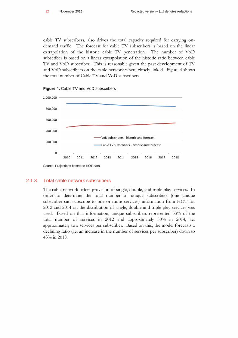
cable TV subscribers, also drives the total capacity required for carrying on-
demand traffic. The forecast for cable TV subscribers is based on the linear
extrapolation of the historic cable TV penetration. The number of VoD
subscriber is based on a linear extrapolation of the historic ratio between cable
TV and VoD subscriber. This is reasonable given the past development of TV
and VoD subscribers on the cable network where closely linked. Figure 4 shows
the total number of Cable TV and VoD subscribers.
Figure 4. Cable TV and VoD subscribers
Source: Projections based on HOT data
2.1.3 Total cable network subscribers
The cable network offers provision of single, double, and triple play services. In
order to determine the total number of unique subscribers (one unique
subscriber can subscribe to one or more services) information from HOT for
2012 and 2014 on the distribution of single, double and triple play services was
used. Based on that information, unique subscribers represented 53% of the
total number of services in 2012 and approximately 50% in 2014, i.e.
approximately two services per subscriber. Based on this, the model forecasts a
declining ratio (i.e. an increase in the number of services per subscriber) down to
43% in 2018.
0
200,000
400,000
600,000
800,000
1,000,000
2010 2011 2012 2013 2014 2015 2016 2017 2018
VoD subscribers - historic and forecast
Cable TV subscribers - historic and forecast

Redacted version – […] denotes redactions November 2015 13
Figure 5. Unique subscribers on cable network
Source: Projections based on HOT data
2.2 Forecasting service usage
The dimensioning of the network is not just based on the number of subscribers
but primarily the result of the traffic those customers generate and the capacities
required for provisioning this. The following sections set out the usage in form
of traffic or capacity requirements on a per subscriber or total capacity basis.
2.2.1 Voice traffic
The voice services covered in the model include all types of calls, disaggregated
into the following categories:
On-net fixed calls;
Calls to and from other fixed and mobile numbers;
International calls (incoming and outgoing); and
Other calls.
Historically, demand for calls on HOT’s network has developed differently for
each type of call. This is both because competition for these services has
developed differently (especially for international calls) and because mobile
services have grown in importance.
Changes in traffic volumes can occur for two reasons. Firstly, total traffic
changes because the number of customers changes. And secondly, changes in
traffic occur due to changes in customer behavior. To effectively isolate these
two effects, we forecast the traffic for different types of calls on a per subscriber
basis. The total voice traffic in any given year is then given by the forecast traffic
per subscriber multiplied with the forecasted number of voice subscribers.
Figure 6 shows the total voice traffic for the modeled period.
0
200,000
400,000
600,000
800,000
1,000,000
1,200,000
1,400,000
2012 2013 2014 2015 2016 2017 2018

14 November 2015 Redacted version – […] denotes redactions
Figure 6. Total annual voice traffic (bn minutes)
Source: Projections based on HOT traffic
2.2.2 Broadband capacity
Broadband services in Israel consist of xDSL based services over Bezeq’s
network and Cable based services from HOT. The network dimensioning of the
cable network is therefore based on the number and capacity of the cable
broadband services it provides. These services are offered with different upload
and download speeds and the speed of a service will typically impact the capacity
required for that service on the network.
The forecast of broadband traffic is based on the effective interconnection
capacity between network operators and ISPs in Israel. Due to the structure of
the market with network operators and ISPs as different companies, this data
provides a longer, more consistent trend of the effective capacity required on the
network. Additionally, it captures the actual usage of network capacity, rather
than extrapolating based on nominal broadband speeds. The data in the model is
the same that was used in the fixed bottom-up model7 complemented with the
most recent measurements from January 2015 which supports the general trend
previously considered. This is further explained in Levaot – Gronau
Recommendations concerning wholesale services pricing over Hot's network.
7 This is based on an average of all broadband subscribers in Israel as measured at the point of
interconnection between ISPs and network operators.
-
1.00
2.00
3.00
4.00
5.00
6.00
2010 2011 2012 2013 2014 2015 2016 2017 2018

Redacted version – […] denotes redactions November 2015 15
Figure 7. Core network capacity per broadband subscribers (Mbps)
Source: Projections based on level and growth of ISP interconnect capacity and international benchmark of
broadband capacity growth
In addition to the core network capacity, the model considers the provisioned
capacity in the access part of the network. This is necessary to dimension the
broadband specific equipment at the headend (CMTS) and the number of
channels required for broadband on the access network. This is done by linking
the current amount of access specific capacity and the capacity on the core
network. The most recent available information for 2014 suggests a configuration
of customer premise equipment of 8 channels for the downstream and 4 for the
upstream. This is based on the configuration of mass market customer premise
equipment (CPE) which was updated to 8 and 4 channels in 2013. In addition,
HOT stated for 2014 its plan to upgrade the cable network by further
segmentation the service groups (Hot’s Upgrade Project).The Upgraded network
dimensioning provides one downstream segment for broadband services to 1000
customers while an upstream segment is provided to 500 customers. The MOC
is aware that extensive areas still don’t match those principles, i.e. the actual
dimensioning in most areas on average is one upstream and downstream segment
to 2000 customers but, in the context of developing a notional network model,
considers it appropriate to model the entire network based on the best practice
principle, which corresponds to Hot's planned dimensioning.8 8 channels at 50
Mbps per channel imply an average downstream capacity of 0.4 Mbps per
subscriber in the access network; 26% higher than the core capacity in 2014.
This factor (1.25) is then used to estimate access capacities on the basis of the
core capacity forecast set out in Figure 7 above.
8 We note that considering this upgraded deployment allows to disregard temporary capacity
limitations in the current network.
-
0.20
0.40
0.60
0.80
1.00
2015 2016 2017 2018

16 November 2015 Redacted version – […] denotes redactions
Finally, for estimating the number of channels in the access network it is also
necessary to consider upstream traffic separate from downstream traffic. Current
offers with 5 Mbps maximum upstream traffic suggest that the network provides
a maximum capacity of 72 Mbps of upstream traffic. This is based on the fact
that the current upstream network is modulated at 16 QAM assuming channel
bandwidths of 6.4 MHz. At 500 customers covered per service group, this
implies an average provisioned capacity of 0.14 Mbps or 36% of downstream
capacity in the access network.
The model assumes that these ratios remain constant and forecasts the amount
of access downstream and upstream capacities by applying ratios of 1.25 and 1.25
x 0.36 to the core downstream capacity forecast set out in Figure 7 above
respectively.
2.2.3 Broadcasting capacity
The capacity required for TV services depends on the types and number of
channels transmitted by the cable operator. It is independent of the number of
subscribers on the network but requires the same capacity on every access
segment of the network (the group of households connected on a final segment
of coaxial cable).
The model distinguishes 4 types of TV channels, SD, HD, 3D and interactive.9
The number of channels is based on forecasting the historic number of channels
on HOT’s network for each type separately:
SD channels are expected to remain at 163; the same as currently in
2014 and similar to the average between 2012 -2014.
HD channels are expected to remain at 22 based on the same principle
as SD channels.
One 3D channel was available in 2010 but has since been discontinued
and the model assumes that no such channels are broadcasted.
Interactive channels have decreased from initially 32 in 2010 to 18 in
2013 and 2014. The model therefore is based on a forecast of 18
channels.
Digital channels are assumed to require the following bandwidths based on
information provided by HOT:
SD – 3.4 Mbps
9 The current network still broadcast analogue channels. However, this service and corresponding
requirements are not included in the model. This is because the provision of analogue channels will
terminate in 2015.
Redacted version – […] denotes redactions November 2015 17
HD – 6.8 Mbps
3D – 6.8 Mbps
Interactive – 6 Mbps
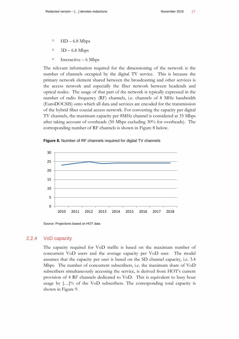
The relevant information required for the dimensioning of the network is the
number of channels occupied by the digital TV service. This is because the
primary network element shared between the broadcasting and other services is
the access network and especially the fiber network between headends and
optical nodes. The usage of that part of the network is typically expressed in the
number of radio frequency (RF) channels, i.e. channels of 8 MHz bandwidth
(EuroDOCSIS) onto which all data and services are encoded for the transmission
of the hybrid fiber coaxial access network. For converting the capacity per digital
TV channels, the maximum capacity per 8MHz channel is considered at 35 Mbps
after taking account of overheads (50 Mbps excluding 30% for overheads). The
corresponding number of RF channels is shown in Figure 8 below.
Figure 8. Number of RF channels required for digital TV channels
Source: Projections based on HOT data
2.2.4 VoD capacity
The capacity required for VoD traffic is based on the maximum number of
concurrent VoD users and the average capacity per VoD user. The model
assumes that the capacity per user is based on the SD channel capacity, i.e. 3.4
Mbps. The number of concurrent subscribers, i.e. the maximum share of VoD
subscribers simultaneously accessing the service, is derived from HOT’s current
provision of 4 RF channels dedicated to VoD. This is equivalent to busy hour
usage by […]% of the VoD subscribers. The corresponding total capacity is
shown in Figure 9.
0
5
10
15
20
25
30
2010 2011 2012 2013 2014 2015 2016 2017 2018

18 November 2015 Redacted version – […] denotes redactions
Figure 9. Peak capacity required for VoD content (Mbps)
Source: Projections based on HOT data
2.2.5 Multicast traffic
Consistent with the fixed network model, the cable model includes a wholesale
broadcasting service for the provision of TV channels by access seekers. This is
in accordance with a policy decision by the MOC which is set out by the Ministry
under separate cover.10. The model therefore also estimates the cost of wholesale
multicast traffic on the assumption (consistent with those considered in the fixed
network model) that this consists of 4 standard definition TV channels each of
which has a capacity of 2.6 Mbps11. As such, the model assumptions and
corresponding costs of the service may be revised in response to any significant
changes in the technical specification or increase in demand of the service, in
terms of number of TV channels.12
10 See BSA & Telephony Service File, incorporated into Hot's License, available at
http://www.moc.gov.il/sip_storage/FILES/3/3963.pdf .
11 This is different from HOT’s own SD channels (3.4 Mbps) because the transmission is carried out
over the IP stream parallel to broadband traffic (not HOT’s system for delivering digital TV
channels). We therefore consider it more appropriate to apply the same technical assumptions for
delivering the service used in the fixed network model.
12 Contrary to the assumptions made in the fixed network model (i.e. delivery of the multicast signal to
1000 MSANs) the HFC model assumes delivery of the signal to all optical nodes. This is because
traffic on the HFC network is less costly and with costs similar to those in the fixed network model,
delivering to all households would be commercially viable for access seekers.
0
100,000
200,000
300,000
400,000
500,000
2010 2011 2012 2013 2014 2015 2016 2017 2018

Redacted version – […] denotes redactions November 2015 19
3 Cable network structure
The model derives equipment and infrastructure requirements of a modern cable
network operator using a hybrid coaxial fiber access network and DOCSIS 3.0
standard for the provision of broadband, voice and audiovisual services. The
structure of the current cable network in Israel is used as a template for that
network. In particular, we have taken the number of network nodes largely as
given.13 The broad structure of the network is set out in Figure 10 below.
Figure 10. HFC network structure
13 This mostly resembles a “scorched node” approach. The network topology is defined as the
established network as “anchor asset”. That is, it will not be feasible in the medium term to reduce
the number of sites. The equipment located at each node is optimized to minimize the cost of the
network.
Master-headend
= Points of interconnection
Headend Headend
CMTS
IP
Core
Aggre
gation
CMTS
IP
Edge
Aggre
gationRFGW CMTS
IP
Edge
Aggre
gationRFGW
RFGW
Optical Nodes
IP
Edge

20 November 2015 Redacted version – […] denotes redactions
Based on this overall structure, the model distinguishes between the access and
the core part of the network. The access part is based on the current number of
optical nodes (ON) and connected cables with the downlink to customer
premises based on coaxial cables and the uplink to headends based on fiber optic
cables. The infrastructure and equipment in this part of the network is passive.
Active equipment is located in headends and considered as part of the core
network. Again, the current number of headends forms the basis of the network
modelling with 18 headend sites and 3 master-headends (a subset of the 18
headend sites). Headends are considered to be placed in areas where the
coverage of the aggregate customer base requires along with the CMTSs, a larger
amount of active equipment including parts of the core IP network. Master-
headends are considered to contain all of the above and additional core IP
routers.
Radio frequency gateway (RFGW) equipment is used in headend locations to
achieve a greater downstream port density to aid in the efficient coverage of the
areas in Israel. In other words, the use of an RFGW enables the use of specific
CMTS equipment with greater port density.
In addition to the number of nodes considered for the network, the linkage
between nodes impacts the dimensioning and costs of the network equipment.
The corresponding assumptions which are broadly based on the current cable
network and consistent with standard engineering rules are set out in below.
Table 2. Equipment links
Equipment/Location Links
Customer premise The customer premise is passed by a single coaxial cable connected to an
optical node – this is considered to be an access segment. (The model
further distinguishes downstream and upstream segments for the
dimensioning of headend equipment – these segments aggregate
customers from several access segments. The details of this aggregation
are set out in section 3)
Optical nodes Each linked by optical fiber to one headend
Headend - RFGW An RFGW is required in headend locations and links the broadband, voice,
wholesale TV downstream traffic to the optical nodes receiving the traffic
from the CMTS through an aggregator.
Headend - Aggregator Located between CMTS and RFGW to ensure an efficient use of port
RFGW port capacities
Headend - CMTS Each linked to two edge routers
Headend - IP edge Edge routers are linked to two IP core routers
Master-headend - IP core Core routers are meshed

Redacted version – […] denotes redactions November 2015 21
Each link is dimensioned to carry all the traffic between the equipment. This
configuration, which corresponds to Hot's submissions concerning the one used
in HOT's network, is efficient in the sense that the individual layers are needed to
concentrate traffic and the equipment employed at each layer is not excessive.
Further, the network provides both diverse routing and capacity resilience - both
features of an efficient and reliable network.


Redacted version – […] denotes redactions November 2015 23
4 Network dimensioning
This section describes the approach to dimensioning the cable network. For
conceptual reasons, this is done separately for the access and core network. For
the purpose of this description, we consider the access network to consist of the
coaxial part of the network up to the optical node. The core network consists of
the optical nodes and fibers to the headends and equipment and infrastructure in
and between headends. Prior to setting out the dimensioning of the network we
describe the approach for determining the capacity required for the provision of
the services on the network. This forms the input to the dimensioning of the
network and the allocation of costs to services.
4.1 Determining service capacity requirements
This section describes how the model determines the network capacity
requirements from service demand inputs.
To dimension different types of equipment and allocate costs to services, we
established for each network element the peak capacity the equipment needs to
handle. This is the capacity required for carrying the amount of traffic at the
time when the sum of traffic generated by all services is highest. This requires a
conversion of forecast demand to peak capacity. The network is then
dimensioned to carry this peak capacity, also taking account of maximum
utilisation levels and redundancy and resilience assumptions for all equipment
types.
The cable network considers two types of capacities; RF Channels and Megabit
per second (Mbps). This is because different network equipment is driven or its
usage expressed by either of these measures.
4.1.1 Capacity requirements for voice services
The model considers different types of calls based on the information considered
in the demand forecast and their use of the network. The voice minutes for each
type of call are converted to capacity in the busy hour by using the following
assumptions:
1. the share of traffic in the busy hour by type of service at […]% based on
information from HOT and similar to the busy hour traffic in Bezeq’s
network;
2. adjustment for holding time of 12s and the percentage of unsuccessful
calls at 23%; and
3. an uplift for variations in the level of traffic over the course of the week
and year of 15%.
24 November 2015 Redacted version – […] denotes redactions
The latter two are based on international precedent (as a result of HOT not
providing corresponding data) for uplift factors and consistent with the
assumptions made in the fixed bottom-up model.
In the next step, the model determines the capacity requirement for each type of
service at the different network elements. Different calls use the network
differently. The extent to which a call uses different network elements is
reflected in routing factors14. Off-net calls are generally considered to use
relevant network elements once. On-net calls will generally use many network
elements twice as intensively as off-net calls.
The model assumes that the bandwidth of a voice call is 98.74 Kbits per second.
This is based on the use of G.711 protocol with appropriate allowance for
overheads (headers and tags). Hence, multiplying the busy hour minutes with the
call bandwidth for each network element gives the capacity requirements (in
kbps). Dividing these totals by 1,000, gives quantities in Mbps.
A further adjustment is made to take account of the real time requirements of
voice. For each network element the number of voice related Erlangs was
divided by the number of network units or links to produce Erlangs per unit. A
blocking rate of 0.2% was then applied to determine the actual capacity needed
to ensure a satisfactory quality of service.
For the dimensioning and cost allocation of the access network, the model also
requires quantifying the number of channels services occupy in the access part of
the network. This is because, the requirements for RF channels is the primary
driver for the use of the hybrid fibre coaxial access network. The number of
channels attributable to voice is based on the basic configuration of the current
cable network which rests on customer premise equipment supporting the use of
8 downstream and 4 upstream channels. The voice service is part of the traffic
that is carried over these primary channels and their amount is calculated based
on the voice capacity requirements (after prioritisation) as a share of total data
related capacities (which in addition to voice consist of broadband and wholesale
broadcasting capacities). For example, in 2015 the capacity required for voice
services as calculated in the model (after prioritisation) is approximately 3.4 Gbps
while other downstream and upstream traffic sharing the same groups of
channels account for approximately 39215 Gbps and 137 Gbps respectively. This
14 A routing factor shows the extent to which different services use network elements.
15 Broadband plus multicast

Redacted version – […] denotes redactions November 2015 25
results in a total number of 383 channels16 being attributed to voice services
(across all access segments in the network).
4.1.2 Capacity requirements for broadband service
As with voice traffic, busy hour broadband traffic was used for the dimensioning
of core network equipment. Since average busy hour usage was provided in kbps
no further transformation was required but to calculate requirements in Mbps by
dividing by 1,000 and 1,000 again to arrive at Gbps. The same principle as set
out for voice above is used for calculating the channels attributable to
broadband. For 2015, total broadband upstream and downstream capacities in
the access network of 380 and 137 Gbps respectively imply that approximately
54,000 RF channels across all access segments are attributed to broadband.
4.1.3 Capacity requirements for broadcasting and VoD services
The broadcasting capacity was calculated in Mbps and RF channels and is already
that required in the busy hour due to its broadcasting characteristics, i.e. due to
the nature of the service, the full capacity of all broadcasting channels is
constantly required. The number of RF channels required is based on the
capacities set out in section 2.2.3 and the equivalent broadband capacity of
50Mbps per 8 MHz channel but taking account of a 30% capacity reduction for
overheads required when broadcasting TV channels. Based on these
assumptions, the total number of channels attributed to TV (following the
assumptions set out for voice earlier) is approximately 119,000 channels across all
access segments in 2015.
The VoD demand is also already expressed in busy hour Mbps and no further
conversion is required to calculate the total capacity. For the number of channels
on the access network, the model takes into account that dedicated channels are
used for providing this service (i.e. contrary to providing the service as part of the
broadband data stream). The usage and capacity assumptions imply that the
average busy hour usage per access segment is approximately […] Mbps in 2015
or […] concurrent VoD streams per access segment. Applying a similar
prioritisation as for voice traffic implies 43 streams in the busy hour or
approximately 146 Mbps or 5 RF channels. This implies a total of approximately
23,000 channels across all access segments in 2015.
16 The total number of channels considered for the dimensioning and cost allocation is based on the
number of optical nodes and the number of upstream and downstream channels configured in the
hardware (4 and 8 channels respectively). This results in a total of approximately 59,000 channels.
across all optical nodes for 2015; i.e. 8 x 4929 = 39,432 downstream channels and 4 x 4929 = 19,716
upstream channels.

26 November 2015 Redacted version – […] denotes redactions
VoD demand and Cable TV content are partly considered to be provided over
dedicated core network equipment while sharing the access equipment and
infrastructure with broadband and voice traffic. While the second is taken into
account by calculating the required number of channels on the access network (as
set out above), the first is not explicitly modelled due to the fact that none of the
services costed in the model are provided over the relevant types of equipment.
4.1.4 Capacity requirements for wholesale broadcast service (multicast
application of BSA service).
The wholesale broadcasting capacity is equally required on a permanent basis,
similar to the TV service. The calculated capacity in Mbps is therefore already
that required in the busy hour. Given that the service is provided as part of those
channels also used for the provision of broadband and voice services, the
number of channels attributed to wholesale broadcasting is determined in the
same way as for voice and broadband services. For example, the total number of
channels attributed to the wholesale broadcasting services is approximately 1,100
channels across all access segments.
4.1.5 Applying the capacity requirements in the model dimensioning
The process set out above is carried out for each year individually converting
service demand to capacity requirements. These requirements form the primary
input to the network dimensioning, although primarily for the core network) is
set out in section 4.3 after the dimensioning of the access network which is set
out in the following section.
4.2 Access network dimensioning
The dimensioning of the access and core networks is based on the analysis by the
Survey of Israel using GIS data of roads and buildings and locations of the
headends and optical nodes in Israel. The survey was used to dimension the core
and access network infrastructure (duct and trench) due to the interdependency
of the two segments of the network (the dimensioning of the equipment of the
core network is covered in the following section).
The survey estimates the distance between the 18 headends and the 4,553 optical
nodes. We also used the estimates of the primary network measured by the
survey of Israel in relation to the fixed network model, for some sharing
assumptions rely mainly on types of road (inter/inner – city). The length of the

Redacted version – […] denotes redactions November 2015 27
access network is the length of the network to reach the customer premises
where they are not already connected by the primary or secondary network.17
This approach implies that some of the trench considered by the Survey of Israel
as secondary or primary trench is also used as access trench. This sharing is
taken into account when considering the total length and cost of the access and
core networks.
The data provided by the survey and further assumptions made in relation to the
modelling of access and core infrastructure are set out in Table 3 below.
Table 3. Data and assumptions* considered for core infrastructure dimensioning
Parameter Value
Length of the total core network) 6,765 km
Length of core network between municipalities (primary network)
Of which is the length between headends
3,711 km
1,096 km
Length of the network between municipalities and optical nodes (secondary network) 3,054 km
Length of the access network (links from optical nodes to customer premises) 17,497 km
Number of optical node locations 4,553
*Degree of sharing between access and primary network 5%
*Degree of sharing between access and secondary network 100%
*Degree of sharing between primary and secondary network 0%
Number of municipalities covered in the study 927
Source: Survey of Israel, SoI for the cable network model, Modelling assumptions
The assumptions about sharing have been determined in the following way:
For the fixed network model, the Survey of Israel, estimated a primary trench
network connecting 927 municipalities through intercity roads. We consider
this estimate of the trench network as part of this model as a subset of the
core trench length estimated by the Survey of Israel for the HOT network
structure. This network leads through the municipalities, therefore covering
also some of the roads that require an access network trench. However, the
17 The principles of this approach are outlined in Survey of Israel's report "Estimating Efficient
Infrastructure Length, Based on Hot Telecom's Infrastructure", November 2015 ( henceforth "SoI
for the cable network model")
28 November 2015 Redacted version – […] denotes redactions
largest part of this part of the trench network would be located between
municipalities without any sharing with the access network. We have
therefore assumed that only 5% of the primary network is shared with the
access network. This is consistent with the assumptions made in the fixed
bottom-up model.
The secondary trench network (estimated as the difference between the
primary network length and the total core network length) connects the
primary trench network to the optical node locations. As such, the trench is
likely to be fully located in an inhabited area (i.e. given that the primary
trench already leads through the municipalities) suggesting that 100% of the
secondary trench would be shared with the access network. Again this
assumption is consistent with that made in the fixed bottom-up model.
Due to the principles applied when constructing the overall network (the
Survey of Israel first measured the primary trench, then the secondary trench
incrementally to reach the optical node location) there is no sharing between
the primary and secondary trench network.
Based on the information provided by the Survey of Israel and the assumptions
outlined above, the gross length of the access trench considered in the model for
the base year (2015) is approximately 21,000 km. The model assumes that some
degree of access network growth takes place on the basis of the historic
expansion of urban roads as evident from CBS18 data implying an annual growth
of 0.8%. This growth is also considered to drive an increase in the number of
optical nodes as well as the length of the secondary network linking the optical
nodes with the primary network based on the ratios between the lengths of the
access and secondary networks and the number of optical nodes in 2014.
The model then estimates the overlap of core and access networks and on that
basis the requirements for ducts and cables. In relation to the dimensioning of
the infrastructure network, the model estimates the costs of a notional network
operator. This implies that infrastructure that HOT is currently renting from
Bezeq is considered as an actual investment assuming the same specifications as
for the rest of HOT’s infrastructure network.
Further elements of the access network are estimated in the following ways:
The model considers two duct bores for that part of the trench that is solely
used for Access or Core. This assumption is based on the requirement to
include in the model empty ducts for infrastructure access services. Parts of
18 Central Bureau of Statistics
Redacted version – […] denotes redactions November 2015 29
the network shared between the core and access networks are
correspondingly modeled using 4 duct bores (two for access, two for core).
The requirements for coaxial cable in the network are based on the gross
length of the access network and the length of coaxial cables including home
wiring provided by HOT. For 2014, this equates to a ratio of approximately
[…] between coaxial cable and gross access trench length. This ratio is then
used to estimate the length of the coaxial cable in years after 2014 given that
the access network length increases over time. The type of coaxial cables is
based on information provided by HOT according to which approximately
30% is used for connecting to the home and is based on RG11 type cable
while the remaining length is based on 540 and 860 type cables in equal
proportions.
The model further considers amplifiers and branching points in the access
network. Both are based on information provided by HOT which equate to
branching points every 70m of the access network and amplifiers every
440m. The resulting number of branching points is consistent with the
relatively low ratio of coaxial cable to access trench19 while the length
between amplifiers is consistent with general engineering principles also
evident from information in one similar model20.
4.3 Core network dimensioning
The volume of each type of network equipment included in the model is typically
determined by the number of nodes in the network, capacity requirements and
assumptions for equipment modularity, utilization and resilience. The model
determines the network element requirements for any given year given these
requirements and assumptions. However, the model also takes into account that
the network equipment is not just brought in service instantaneously when
capacity is required. We therefore take account of build-ahead requirements, i.e.
investments are carried out a year prior to the network being required to meet the
respective demand.
We distinguish between 4 types of network equipment as illustrated in Figure 10
earlier:
optical nodes;
19 A larger number of branching points enables the network operator to decrease the length of
individual coaxial cables to customer premises.
20 http://danishbusinessauthority.dk/file/234415/kobber%2c_kabel-
tv_og_fibre_%28dong%29_zip.zip
30 November 2015 Redacted version – […] denotes redactions
CMTS and associated headend equipment (aggregators and radio
frequency gateways (RFGW));
core IP equipment; and
infrastructure.
The following sections set out each type in more detail.
4.3.1 Optical node
Optical nodes are used to convert the optical transmission of RF channels over
fiber to electrical transmission over coaxial cable for the final transmission and
connection to customers. The number of optical nodes in 2014 is based on the
information from the current cable network in Israel and is considered in the
model on the basis of a ratio between the current length of the access network
and the number of optical nodes. This implies that the number of optical nodes
is gradually increasing as the coverage of the network also increases. In principle,
there is also a potential need for optical nodes to increase as a result of higher
capacity demands for subscribers. However, there are two reasons why we
believe that this is unlikely to happen over the modelled period:
The current number of subscriber per optical node is comparably low
with approximately […] in HOT’s network. For example, the model in
Denmark considers an average of 350 subscribers per optical node.21
According to HOT, its current network rollout principles for
broadband are based on a grouping of 1,000 subscribers per
downstream segment. In other words, one service group of eight RF
downstream channels covers more than 3 optical nodes on average. As
such, the network is able to provide further downstream capacity by
reducing the number of optical nodes per downstream segment. Only
after the downstream capacity requirements exceeds the capacity
available from defining a single service group for every optical node
may the need arise for further segmentation, i.e. splitting an optical
node into two and thereby reducing the number of subscribers and
hence capacity required per node.22 Under the forecasts considered in
this model, this need does not arise.
21 http://danishbusinessauthority.dk/file/234415/kobber%2c_kabel-
tv_og_fibre_%28dong%29_zip.zip
22 This is only the case if the same customer premise equipment as today is used. Current cable
modems support channel bonding of 8 downstream and 4 upstream channels. Future modems are
planned to support 16 and 4 as well as 24 and 8 channels greatly reducing the need for further
segmentation as broadband capacity continue to increase.
Redacted version – […] denotes redactions November 2015 31
The number of nodes then also determines the number of coaxial segments to
customers and fiber uplinks to the headend which are equal to the number of
optical nodes. The model further dimensions equipment required for optical
transmission and electric to optical conversion at the headend. This is covered
separately for the upstream and downstream optical fiber at a ratio of 2 per
upstream receiver and 4 per downstream transmitter based on the equipment
modularity used by HOT.
4.3.2 CMTS and related equipment
The CMTS at the headend is responsible for managing broadband subscribers
and traffic. Together with the CMTS equipment we consider equipment
associated with the function of the CMTS, in particular the RFGW and the
aggregator (consolidating traffic between the RFGW and CMTS).
Dimensioning the CMTS equipment
For dimensioning the CMTS equipment, the model takes primary account of the
uplink and downlink traffic carried between the core and access network. The
relevant capacity requirements are those for the access and the core network set
out in section 2.2.2 for the downlink and uplink respectively. This is because, the
CMTS equipment provides separate ports for upstream and downstream traffic
and the dimensioning therefore considers the corresponding capacities separately.
The equipment is dimensioned by the number of channels required for upstream
and downstream traffic. Downlink cards (cards directed towards the access
network) have different channel capacities for downstream and upstream traffic.
The number of cards are dimensioned according to the maximum number of
channels required based on either downstream or upstream capacities.
Downstream ports are connected to aggregation equipment for combining
downstream broadband traffic from several CMTS. Downstream ports at the
CMTS are paired for providing redundant links to the aggregator. Upstream
traffic terminates directly on the upstream ports of the CMTS from the
RF/optical transcoder equipment.
While the precise allocation of optical nodes to headends is not known, the
model considers that headends will typically serve a varying number of optical
nodes. To reflect that variability, the model attributes the populations at the
locations of the current 18 headends to those headends. In addition, these
headends would also be assumed to cover a share of the residual population in
locations other than those with headends which is assumed to be covered by
those headends in equal shares.
The number of optical nodes attributed to these headends is then based on the
number of subscribers attributed to each locality (the model assumes that
subscribers are proportionate to the number of inhabitants) divided by the
32 November 2015 Redacted version – […] denotes redactions
average number of subscriber per optical node. In 2015, the number of optical
nodes per headend ranges between […] and […].
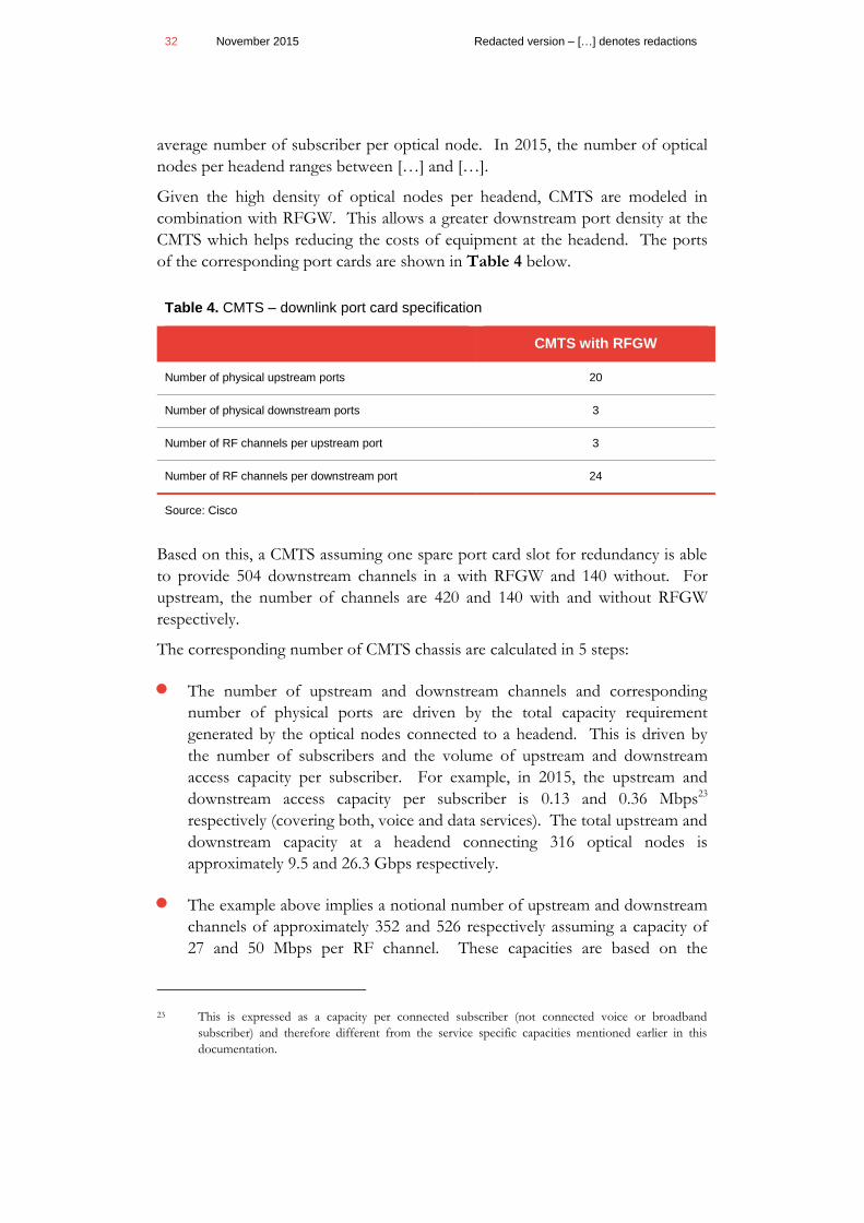
Given the high density of optical nodes per headend, CMTS are modeled in
combination with RFGW. This allows a greater downstream port density at the
CMTS which helps reducing the costs of equipment at the headend. The ports
of the corresponding port cards are shown in Table 4 below.
Table 4. CMTS – downlink port card specification
CMTS with RFGW
Number of physical upstream ports 20
Number of physical downstream ports 3
Number of RF channels per upstream port 3
Number of RF channels per downstream port 24
Source: Cisco
Based on this, a CMTS assuming one spare port card slot for redundancy is able
to provide 504 downstream channels in a with RFGW and 140 without. For
upstream, the number of channels are 420 and 140 with and without RFGW
respectively.
The corresponding number of CMTS chassis are calculated in 5 steps:
The number of upstream and downstream channels and corresponding
number of physical ports are driven by the total capacity requirement
generated by the optical nodes connected to a headend. This is driven by
the number of subscribers and the volume of upstream and downstream
access capacity per subscriber. For example, in 2015, the upstream and
downstream access capacity per subscriber is 0.13 and 0.36 Mbps23
respectively (covering both, voice and data services). The total upstream and
downstream capacity at a headend connecting 316 optical nodes is
approximately 9.5 and 26.3 Gbps respectively.
The example above implies a notional number of upstream and downstream
channels of approximately 352 and 526 respectively assuming a capacity of
27 and 50 Mbps per RF channel. These capacities are based on the
23 This is expressed as a capacity per connected subscriber (not connected voice or broadband
subscriber) and therefore different from the service specific capacities mentioned earlier in this
documentation.
Redacted version – […] denotes redactions November 2015 33
assumption that a newly deployed cable network is capable of operating at
64 and 256 QAM on channels of 6.4 and 8 MHz bandwidths, upstream and
downstream respectively.
4 and 8 upstream and downstream channels form a single upstream and
downstream service group respectively and can provide services to several
optical nodes per service group (independent for upstream and
downstream). Because of that, the numbers of channels calculated in the
previous step need to be adjusted to take into account that service groups
cannot be attributed to a fraction of an optical node. I.e. the number of
optical nodes per service group based on the notional number of channels
may be 4.5. This means that the number of channels must be adjusted in
such a way, that the maximum number of optical nodes per service group
doesn’t exceed 4. Based on the example set out earlier, the increase in the
number of channels in 2015 is approximately 20% for upstream and
downstream, resulting in a total of 424 upstream and 632 downstream
channels.
Based on the dimensions of the CMTS equipment, the number of these
channels drives the number of physical ports required. For example, based
on the channels calculated above, the number of physical ports required are
142 for upstream and 27 for downstream. Based on the technical
dimensions of the port cards considered, the card requirements are 8 based
on upstream and 9 based on downstream. The maximum of the two drives
the total number of slots required (i.e. in the case above 9). This is because
upstream and downstream ports are provided on the same card.
Finally, the total number of required slot cards drives the number of CMTS
chassis. Based on the example above, a single chassis is required based on
the maximum number of slots of 8 assuming that one slot remains empty
for redundancy.
Further steps involve the dimensioning of uplink cards to IP equipment
which is based on the total downstream capacity required.24 The model uses
the core downstream traffic as upstream will typically be less than
downstream and transmission links in the core network are bidirectional
providing the same capacity up- and downstream.
24 Taking account of a maximum utilization rate of 80%, which is equal to the widely accepted
utilization rate of core network equipment.

34 November 2015 Redacted version – […] denotes redactions
The equipment considered for headends, consistent with the current cable
network, includes three additional types of equipment prior to the fibre optic
downlink to the optical nodes:
Aggregator: Aggregation equipment at the headend consolidates
downstream ports from the CMTS equipment. This is appropriate given the
downstream output ports at the CMTS (1GE) are of a lower capacity than
the downstream input ports at the RFGW (10GE). The aggregator is
dimensioned according to the number of 1 and 10 GE ports to CMTS and
RFGW and based on the modularity of equipment currently used in the
cable network in Israel.
Radio frequency gateway: The RFGW consolidates downstream channels
prior to transmission over the hybrid fiber coaxial network. The modularity
and equipment set out in the model is based on current equipment in the
cable network in Israel. In line with manufacture specification, all RFGW
are fully equipped with port cards regardless of utilization. However, the
total number of RFGW is still based on the requirements of upstream and
downstream ports and channels although the requirements for the modelled
network and period do not exceed one RFGW per headend location.
Separate CMTS and RFGW also imply a requirement for additional
equipment for the provision of the DOCSIS timing interface. This is
provided by two DTI servers per headend location where the second server
is provided for backup.
Table 5 below sets out the number of assets considered in this section over the
period of the model (after taking account of build-ahead requirements).
Table 5. CMTS and associated equipment in headends
2015 2016 2017 2018
CMTS 34 48 84 84
RFGW 19 19 20 20
Aggregator 18 18 18 18
DTI 36 36 36 36
Source: HFC model
4.3.3 IP routers
IP routers at the headends are responsible for handling traffic between headends
by linking edge IP routers to a set of core IP routers. Core IP routers are

Redacted version – […] denotes redactions November 2015 35
meshed as well as connected to other types of service specific equipment, such as
voice switches and interconnect with other operators, e.g. ISPs.
Every headend has one or more IP routers to transmit broadband and voice
traffic. VoD and HOT’s TV traffic is assumed to be carried over separate
equipment. A scenario for an all IP provision of services might be reasonable to
consider in a future version of the model given that equipment vendors aim to
offer convergence solutions while operators are seeking to simplify their network
structure. However, given the lack of corresponding precedent of all IP cable
networks suggests that rolling out an all IP network does not yet represent a
viable option.
Based on the information provided by HOT at the end of 2014 on the actual
cable network in Israel, the model considers the same type of equipment for the
edge and the core.
Edge routers: The model dimensions the edge routers (i.e. the chassis and
ports) to be able to handle the traffic and ports for downlinks to CMTS and
uplinks to core IP routers In 2015, the model estimates a total of 18 edge
routers, one per headend.
Core routers: The model estimates core routers based on the requirements
for uplinks from edge routers and the assumption that core routers are fully
meshed but also the assumption that at least 3 core router sites are required
for resilience and interconnection. Based on the 2014 to 2018 demand and
modelled edge routers, the model does not estimate more than three core
routers for the entire model period. These are assumed to be located at
different headend sites.
As for CMTS, edge and core routers are dimensioned according to the number
of ports and hence port cards and port card slots required. Each edge router
terminates a number of 10GE downlinks from CMTS taking into account
resilience; i.e. each CMTS links to two edge routers. The number of uplinks to
core routers is driven by the amount of core capacity required25, i.e. further
aggregating the capacity provided over the edge router links and the resilience
assumption of one edge router linking to two core routers. The port
requirements of core routers are driven by the number of those links and the
number of cross links to other core routers assuming that core routers are fully
meshed. The number of ports drives the number of port cards assuming a total
number of 24 10GE ports per port card. The number of port cards then drives
the number of chassis assuming a maximum of 7 available slots, assuming one
slot is kept as spare.
25 Again taking into account a maximum utilizations rate of 80%.

36 November 2015 Redacted version – […] denotes redactions
Table 6 below sets out the number of edge and core IP routers as well as port
cards estimated in the model (after taking account of build-ahead requirements).
Table 6. IP edge and IP core router
2014 2015 2016 2017 2018
Edge IP router 18 18 18 18 18
Edge IP – port cards* 20 23 29 41 41
Edge IP router 3 3 3 3 3
Core IP – port cards* 3 4 6 7 7
Source: HFC model
* The number of port cards in the edge router increase significantly as a result of the increase in the number of CMTS.
The port cards in the core router increase as a result of the significant increase in data traffic.
4.3.4 Infrastructure
The final step in modelling the core network covers the dimensions of the
infrastructure connecting the various nodes in the core network. The
dimensioning of the network is again based on the analysis carried out by the
Survey of Israel.26 Based on this information, the total core network distance is
6,765 km in 2014. The data provided by the survey and further assumptions
made in relation to the modelling of core and access network infrastructure are
set out in Table 7 below.
Table 7. Data and assumptions* considered for core infrastructure dimensioning
Parameter Value
Length of the network between headends 1,096 km
Length of the primary network (major roads between municipalities) 3,711 km
Length of secondary network (links from the primary roads to optical nodes) 3,054 km
Optical node locations considered for estimating length of secondary network 4,553
Number of municipalities covered in the study 927
*Degree of sharing between access and primary network 5%
*Degree of sharing between access and secondary network 100%
*Degree of sharing between primary and secondary network 0%
Source: Survey of Israel, Survey of Israel for the cable network model, Modeling assumptions
26 Survey of Israel's report "Estimating Efficient Infrastructure Length, Based on Hot Telecom's
Infrastructure", November 2015
Redacted version – […] denotes redactions November 2015 37
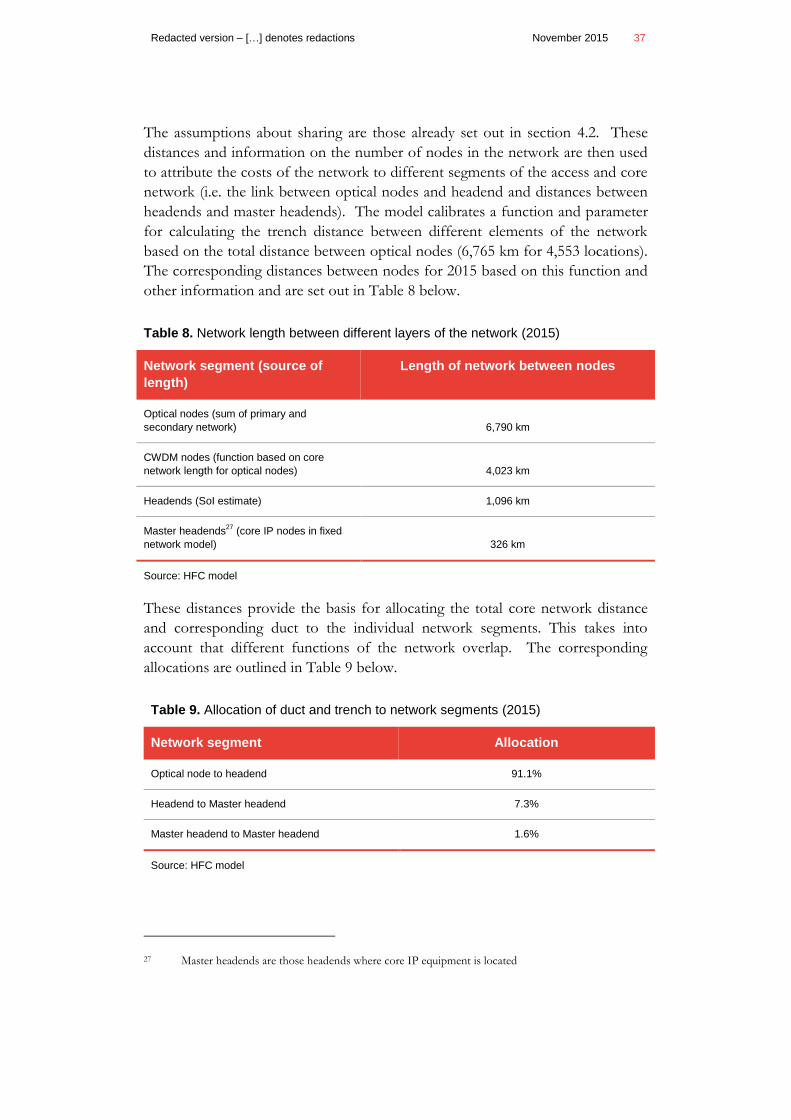
The assumptions about sharing are those already set out in section 4.2. These
distances and information on the number of nodes in the network are then used
to attribute the costs of the network to different segments of the access and core
network (i.e. the link between optical nodes and headend and distances between
headends and master headends). The model calibrates a function and parameter
for calculating the trench distance between different elements of the network
based on the total distance between optical nodes (6,765 km for 4,553 locations).
The corresponding distances between nodes for 2015 based on this function and
other information and are set out in Table 8 below.
Table 8. Network length between different layers of the network (2015)
Network segment (source of
length)
Length of network between nodes
Optical nodes (sum of primary and
secondary network) 6,790 km
CWDM nodes (function based on core
network length for optical nodes) 4,023 km
Headends (SoI estimate) 1,096 km
Master headends27
(core IP nodes in fixed
network model) 326 km
Source: HFC model
These distances provide the basis for allocating the total core network distance
and corresponding duct to the individual network segments. This takes into
account that different functions of the network overlap. The corresponding
allocations are outlined in Table 9 below.
Table 9. Allocation of duct and trench to network segments (2015)
Network segment Allocation
Optical node to headend 91.1%
Headend to Master headend 7.3%
Master headend to Master headend 1.6%
Source: HFC model
27 Master headends are those headends where core IP equipment is located
38 November 2015 Redacted version – […] denotes redactions
Consistent with the assumptions made for the access network, the number of
ducts in the core network is two in areas where the trench is solely used for the
core network and four where the trench is shared with the access network.
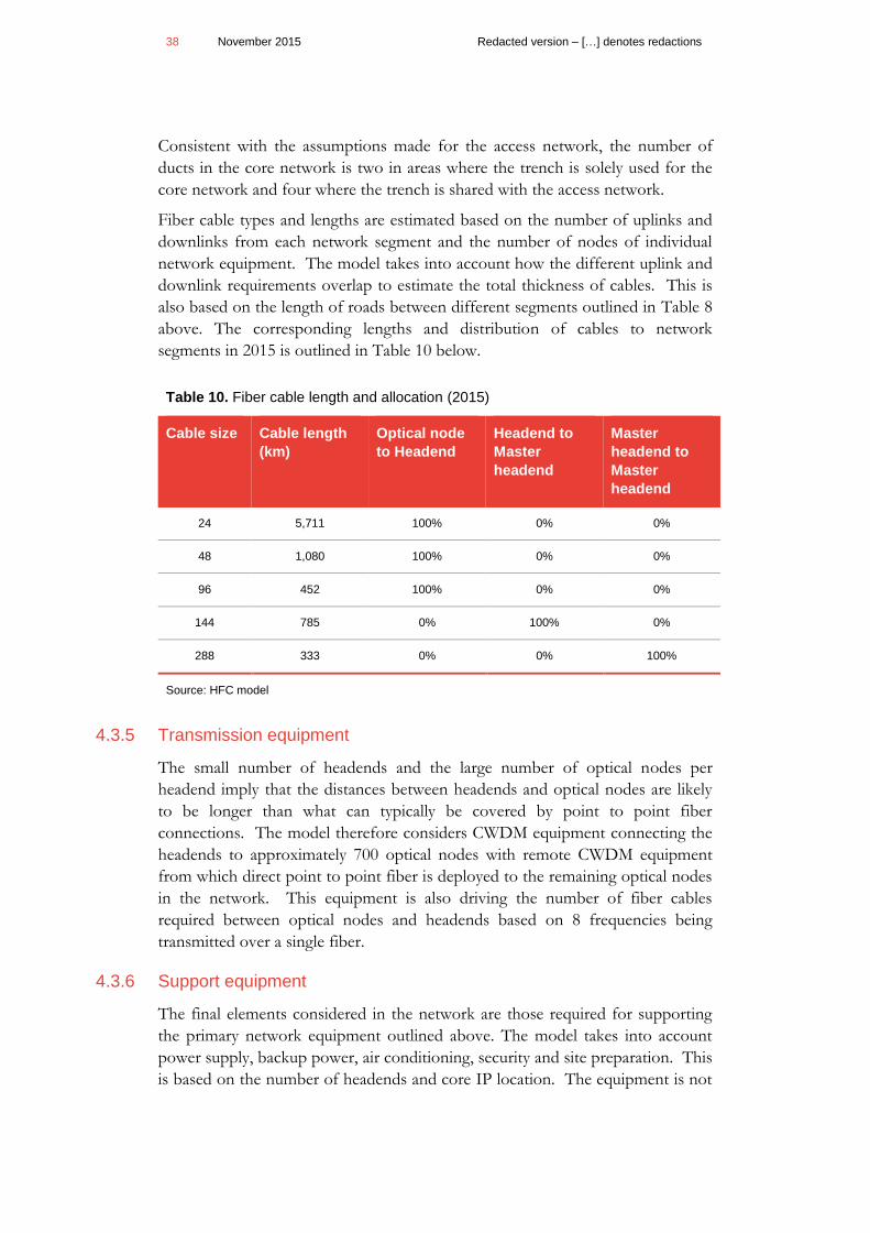
Fiber cable types and lengths are estimated based on the number of uplinks and
downlinks from each network segment and the number of nodes of individual
network equipment. The model takes into account how the different uplink and
downlink requirements overlap to estimate the total thickness of cables. This is
also based on the length of roads between different segments outlined in Table 8
above. The corresponding lengths and distribution of cables to network
segments in 2015 is outlined in Table 10 below.
Table 10. Fiber cable length and allocation (2015)
Cable size Cable length
(km)
Optical node
to Headend
Headend to
Master
headend
Master
headend to
Master
headend
24 5,711 100% 0% 0%
48 1,080 100% 0% 0%
96 452 100% 0% 0%
144 785 0% 100% 0%
288 333 0% 0% 100%
Source: HFC model
4.3.5 Transmission equipment
The small number of headends and the large number of optical nodes per
headend imply that the distances between headends and optical nodes are likely
to be longer than what can typically be covered by point to point fiber
connections. The model therefore considers CWDM equipment connecting the
headends to approximately 700 optical nodes with remote CWDM equipment
from which direct point to point fiber is deployed to the remaining optical nodes
in the network. This equipment is also driving the number of fiber cables
required between optical nodes and headends based on 8 frequencies being
transmitted over a single fiber.
4.3.6 Support equipment
The final elements considered in the network are those required for supporting
the primary network equipment outlined above. The model takes into account
power supply, backup power, air conditioning, security and site preparation. This
is based on the number of headends and core IP location. The equipment is not

Redacted version – […] denotes redactions November 2015 39
estimated as such, but the costs provided by HOT, which were reconciled against
the normative costs used in the fixed model, are divided by the current number
of headends to calculate an average costs which is then applied to the modeled
number of headends. Further detail on this is provided in section 5.
4.4 Network dimensioning outputs
The model generates for each year of the modelled period a list of infrastructure
and equipment units consistent with the demand and corresponding capacity
requirements for that year. In accord with best practices and TSLRIC
methodology, prior to applying unit capex and operating costs, the model takes
into account a build ahead requirement of one year which implies that the costs
in the current year are driven by the equipment and infrastructure demand of the
following year. The corresponding equipment units are then considered in the
network and service costing section of the model, the details of which are
discussed in the following sections.

Redacted version – […] denotes redactions November 2015 41
5 Network costing
The next step in the modelling process is the calculation of total network costs
based on the equipment and infrastructure quantities estimated in the model.
The process follows 4 steps:
calculating annual gross replacement costs;
calculating annual operating expenses;
annualizing gross replacement costs; and
calculating total annual costs.
The inputs to this process are primarily based on the current cable network in
Israel, complemented where necessary with information from other jurisdictions
and assumptions taken in the fixed bottom-up model considered in MOC
Decision.28 For example, this is the case for input costs, such as trenches, ducts
and fibres that are equivalent across both types of networks.
5.1 Calculating gross replacement costs
The gross replacement costs include acquisition and installation costs of the
equipment and infrastructure set out in section 4 of this document. The majority
of the cost inputs to the model are based on information from the current cable
network in Israel. While often inconsistent and in formats different from those
requested from HOT, the information provided was sufficiently extensive to be
able to reliably populate most elements of the costing part of the model when it
was found to correspond with costs incurred by an efficient operator. Data on
cost had been received on a number of occasions between 2011 and 2014.
Where possible and sufficiently comprehensive, the most recent data was used.
Hot also provided, to our and MOC's demands, further clarifications and
explanations to the data it provided. Hence, the cable network model relies less
on benchmark data than the fixed bottom up model.
The following table sets out the data used in the model, the year to which it
relates and the assumptions applied in relation to installation.
28 Final decision concerning wholesale services rates in Bezeq's network, dated 17.11.14. available at
http://www.moc.gov.il/sip_storage/FILES/0/3960.pdf

42 November 2015 Redacted version – […] denotes redactions
Table 11. Infrastructure and equipment cost inputs
Infrastructure /
equipment
Year of cost
information
Source Acquisition
(NIS)
Installation
(NIS)
Trench 2014 2 Israeli operators / consistent
with assumption in fixed cost
model
178,023
Duct 2014 12,100
Coaxial cable,
branching
points and
amplifiers
2012
2013
2013
HOT Coaxial cable […]*
Branching point […]*
Amplifier […]*
Fiber cables 2013 1 operator in Israel and 1
confidential source / consistent
with assumption in fixed cost
model29
Cable - ducted 24 fiber 11,228
Cable - ducted 48 fiber 12,211
Cable - ducted 96 fiber 15,301
Cable - ducted 144 fiber 16,235
Cable - ducted 192 fiber 21,156
Cable - ducted 288 fiber 21,310
Optical node 2014 HOT Cabinet […]
Transceiver^ […] 20%
Optical
transmitter and
receiver (HE)
2014 HOT^ Transmitter […]
Receiver […]
20%
20%
CMTS 2013 HOT^ Chassis - […]
Port cards – […]**
20%
RFGW 2013 HOT^ Chassis - […]
Port cards - […]
20%
Aggregator 2013 HOT^ Chassis - […]
20%
DTI 2013 HOT^ […] 20%
IP edge / core
router
2014 HOT^ Chassis - […]
Module - […]
Ports - […]
20%
Support costs
Headend
(CMTS / RFGW
/ IP)
2012 HOT
Power […]
Backup power […]
Air conditioning […]
Site preparation […]
*averages of several types of equipment
^Acquisition costs based on HOT excluding installation. The installation mark-up has therefore been
based on the assumptions for core network equipment used in the fixed network model.
** additional costs apply based on the number of ports being utilized
29 Fiber jointing costs are based on Danish BU model; consistent with assumptions in fixed BU model.
Redacted version – […] denotes redactions November 2015 43
We made a number of observations in relation to the cost data provided by
HOT:
CMTS/RFGW and associated equipment prices also vary significantly in the
data provided by HOT. Cost information provided for 2011 and 2013
differs significantly. Information provided in 2014 is again different from
those costs previously provided for 2011 and 2013. We have therefore
compared this information against costs of equipment in the Danish
bottom-up model and found that all three data points are lower compared to
those costs. The 2014 cost information is significantly higher and does not
allow to extract the actual discounts HOT may have received over the listed
prices, and hence using the 2014 prices would result in gross overestimation
of network costs. We therefore use the 2013 information in the cable
network model.
Support costs are not based on individual equipment units but rather based
on the costs provided by HOT for the overall functions in its network.
These costs have then been attributed in equal amounts to individual
equipment in headends which results in costs being similar to those
considered in the fixed BU model except for site preparation costs which are
significantly higher. This is likely to be the case because site preparation as
provided by HOT also includes the space required for equipment not
considered in the model (such as VOD, Broadcasting and voice specific
equipment). We have therefore chosen the site preparation cost of IP core
equipment as considered in the fixed BU model. This is reasonable because
the size and amount of equipment is more similar to fixed core IP than
aggregation or IP edge equipment which is more numerous in fixed
networks and therefore typically smaller and less costly in relation to site
preparation.
Based on the assumptions and inputs set out above, the model calculates total
gross replacement costs by multiplying the acquisition and installation unit costs
with the units estimated in the network dimensioning part of the model. The
gross replacement cost for each equipment and infrastructure is then considered
for the calculation of operating expenses and the annual capital costs. This is set
out in the following sections.
5.2 Estimating operating expenses
Operating expenses are primarily based on information provided by HOT in
relation to specific network equipment. The model considers mark-ups applied
to gross replacement costs calibrated to match the 2013 modeled operating costs
with the information provided by HOT for the years 2012 and 2013. The
corresponding mark-ups and total operating expenses have been compared
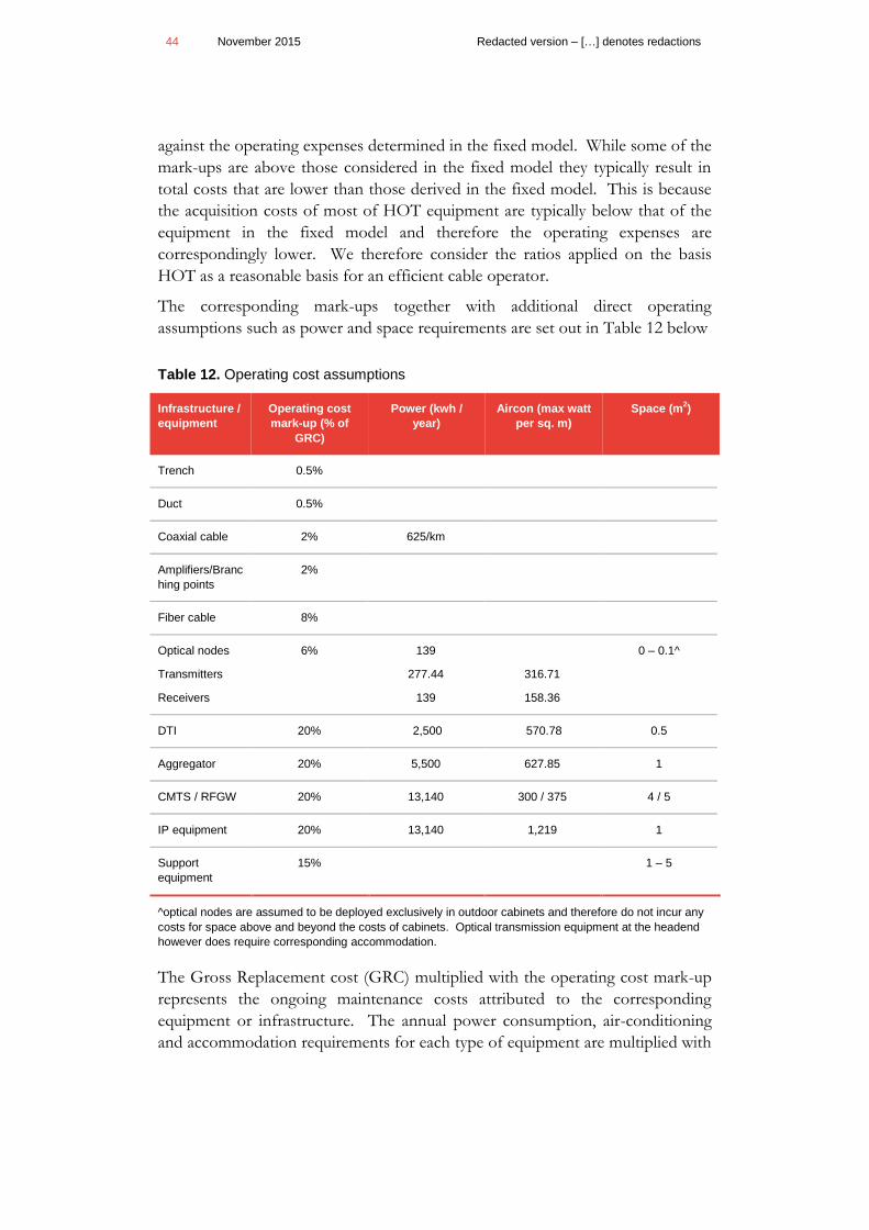
44 November 2015 Redacted version – […] denotes redactions
against the operating expenses determined in the fixed model. While some of the
mark-ups are above those considered in the fixed model they typically result in
total costs that are lower than those derived in the fixed model. This is because
the acquisition costs of most of HOT equipment are typically below that of the
equipment in the fixed model and therefore the operating expenses are
correspondingly lower. We therefore consider the ratios applied on the basis
HOT as a reasonable basis for an efficient cable operator.
The corresponding mark-ups together with additional direct operating
assumptions such as power and space requirements are set out in Table 12 below
Table 12. Operating cost assumptions
Infrastructure /
equipment
Operating cost
mark-up (% of
GRC)
Power (kwh /
year)
Aircon (max watt
per sq. m)
Space (m2)
Trench 0.5%
Duct 0.5%
Coaxial cable 2% 625/km
Amplifiers/Branc
hing points
2%
Fiber cable 8%
Optical nodes
Transmitters
Receivers
6% 139
277.44
139
316.71
158.36
0 – 0.1^
DTI 20% 2,500 570.78 0.5
Aggregator 20% 5,500 627.85 1
CMTS / RFGW 20% 13,140 300 / 375 4 / 5
IP equipment 20% 13,140 1,219 1
Support
equipment
15% 1 – 5
^optical nodes are assumed to be deployed exclusively in outdoor cabinets and therefore do not incur any
costs for space above and beyond the costs of cabinets. Optical transmission equipment at the headend
however does require corresponding accommodation.
The Gross Replacement cost (GRC) multiplied with the operating cost mark-up
represents the ongoing maintenance costs attributed to the corresponding
equipment or infrastructure. The annual power consumption, air-conditioning
and accommodation requirements for each type of equipment are multiplied with

Redacted version – […] denotes redactions November 2015 45
costs of 0.56 NIS, 6.64 NIS and 977 NIS respectively; consistent with the
assumptions in the fixed network model.
5.3 Annualizing gross replacement costs
In setting regulated prices, investment costs need to be recovered over the period
the assets generate revenues for the company, rather than in the year the cost was
incurred. We applied “annuity” and “price tilted annuity” formulae to establish
the annual cost of assets in each year of the modelled period.
The standard annuity formula is applied to passive infrastructure assets reflecting
their importance as bottle-neck infrastructure and the fact that access seekers are
unlikely to seek to establish a parallel infrastructure in addition to those operated
by HOT and Bezeq.
The annuity formulae are used to set a general path for returns (R) on an
investment (I) over the life of the investment (N years). Overall, the initial
investment must be equal to the Net Present Value (NPV – the left hand side of
the equation) of returns over time:
∑𝑅𝑡
(1 + 𝑟)𝑡
𝑁
𝑡=1
= 𝐼
For active network equipment (such as routers) a ‘tilt’ is applied at the rate of
equipment price changes. This takes into account that such equipment costs will
typically decrease over time.
An annuity with a tilt therefore provides the same NPV over the life of the assets
but with the profile of that compensation falling over the life of the asset. The
formula for the price tilted annuity applied in the model is as follows:
𝑅𝑡 = 𝑉𝑟 − 𝑡𝑟𝑒𝑛𝑑
1 − (1 + 𝑡𝑟𝑒𝑛𝑑1 + 𝑟 )
𝑦𝑒𝑎𝑟𝑠
where r is the cost of capital30 and trend the equipment specific price trend and V
the gross replacement costs of the assets.
A price tilted annuity formula was used to ensure an equal spread of costs of
equipment across years with a focus on recovering costs in earlier years if the
price of that asset is expected to decrease and in later years if the price of the
30 The determination of the cost of capital (WACC) is set out in Frontier Economics: "Estimating the
Cost of Fixed call Termination on Bezeq's Network", October 2013, Available at
http://www.moc.gov.il/sip_storage/FILES/3/3383.pdf. For applying the WACC used in the FTR
decision in the cable network model, see Levaot - Gronau Recommendations concerning wholesale
services pricing over Hot's network.

46 November 2015 Redacted version – […] denotes redactions
asset is expected to increase. This reflects the competitive pressure an operator
would face if alternative operators entered the market at any given point of the
modeled period, purchasing equipment at prices expected for that period
For the equipment employed in the cable network, we assume the following price
trends and economic lifetimes as outlined in Table 13.
Table 13. Equipment / infrastructure price trends (real31
)and economic lifetime
Equipment / infrastructure Price trend Economic lifetime
Infrastructure (coax) 0% 30 (15 for amplifiers)
Infrastructure (duct, trench) 0% 40
Infrastructure (fiber) -2.56% 25
Optical nodes / equipment -2.56% 8 (15 for the cabinet)
CMTS/RFGW -2.56% 8
IP -2.56% 8
Support -2.56% 15 (30 for site
preparation)
For calculating annualized capital costs, the model multiplies the gross
replacement costs of each network element with the price tilted annuity factor for
that element.
5.4 Calculating total annual costs of network
equipment and infrastructure
The final step in the network costing section of the model considers common
and indirect operating expenses. These are based on information from HOT and
are expressed in the model as a mark-up to direct annual capital and operating
costs at a level of 13.8%. In other words, common and indirect costs are
attributed to network equipment based on an equi-proportionate mark-up prior
to network cost allocations to services. While this mark-up is higher than the
one applied in the fixed model (10%), the total overhead for the cable network is
approximately NIS 40m lower than that estimated for the fixed network. This is
31 The price trend for trench and coaxial cable is set to zero following the principle of constant input
prices and standard annuity depreciation for passive infrastructure.

Redacted version – […] denotes redactions November 2015 47
because the level of capital investments for the cable network is significantly
lower than those for the fixed network. As overhead costs are unlikely to be
directly related to the technology of the network which leads to those differences
in costs we consider that the higher mark-up are reasonable for the cable
network.
The sum of operating, annual capital and attributed common and indirect costs
are then allocated to services. This is set out in the following section.


November 2015 49
6 Service costing and model results
The final step in the modelling process is to allocate total annual costs of
equipment and infrastructure to services. This section outlines the steps involved
in this calculation by first setting out the process of cost allocations followed by
an overview of the calculation of final wholesale service costs.
6.1 Cost allocation
In cases where a particular type of equipment is solely used to provide a single
service, its costs can be directly attributed to this service. However, in cable
networks, consistent with other telecommunication networks, equipment and
infrastructure are used to provide a range of different services. Hence, the cost of
this equipment and infrastructure needs to be attributed between those different
services. The model attributes these costs according to the intensity with which a
particular type of equipment is used by different services. For example, the fiber
links between headends and optical nodes provide transmission for voice, data
and broadcasting services. Therefore, the costs for fiber and associated
infrastructure and equipment are allocated to the different services relative to
their utilization of the links.
The allocation of costs to services is done in 4 steps:
The costs of equipment and infrastructure are mapped to those network
categories for which a set of routing factors are applied. I.e. there are fewer
network categories than equipment and infrastructure elements in the
dimensioning part of the model.
Each modelled service has a set of routing factors across all network
categories according to its utilization of the network elements.
The demand for all services are multiplied with their respective sets of
routing factors to determine the total service volume for each network
category and finally network category unit cost.
The final allocation of costs to wholesale services is then based on the
consumption of a single wholesale service of these network category units,
again set out by the routing factors for a particular service.
The calculation and results for the final wholesale services are set out in the
following section.

50 November 2015 Redacted version – […] denotes redactions
6.2 Wholesale service costing
The HFC model estimates the costs of the following wholesale services:
bitstream transport;
wholesale subscriber access, and
wholesale broadcasting transport.
The cost estimate for the bitstream transport service includes the costs of the
optical node and optical fiber network to the headend as well as the CMTS and
associated equipment and core IP equipment. The cost is estimated on a per
Mbps basis. Based on the steps set out in the previous section, Table 14 sets out
the costs attributable to the bitstream service in 2015.
Table 14. Bitstream service costs, core element (NIS / Mbps – 2015)
The total core network cost per Mbps based on the table above is around NIS
132. The service also takes into account the costs attributable to channels for
carrying broadband services between the optical nodes and headends. The total
cost added for this element once converted to Mbps is NIS 112 per Mbps.
Finally, applying wholesale specific cost mark-ups of 5.3%32 to the above cost
elements calculates total annual costs per Mbps of around NIS 254 in 2015 or
21.37 NIS per Mbps per month.
The cost estimate for the wholesale subscriber access includes the passive
infrastructure between the optical node and the customers and is expressed as a
32 The wholesale specific mark-up is based on the assumptions in the fixed bottom-up model.
Network elementTotal annual
cost
Total network
volume (Gbps)
Network unit
cost (NIS /
Gbps)
Broadband
service
volume (Gbps)
Broadband
unit cost (NIS
/ Mbps)
Optical node 13,567,399 0 0 0 0.00
DTI 1,123,626 477 2,357 462 3.61
Aggregator 888,326 477 1,863 462 2.85
RFGW 9,167,001 477 19,225 462 29.43
CMTS: Downlink 3,281,577 477 6,879 462 10.53
CMTS: Processor 4,160,848 477 8,722 462 13.35
CMTS: Uplink 2,247,278 304 7,391 302 7.39
Edge router: Downlink 4,564,613 304 15,014 302 15.01
Edge Router: Processor 3,256,328 304 10,714 302 10.71
Edge Router: Uplink 4,113,787 304 13,535 302 13.54
Core Router:Processor 490,571 304 1,615 302 1.62
Core Router: Core Router 1,890,146 304 6,223 302 6.22
Transmission - Coaxial cable 457,019,184 0 0 0 0.00
Transmission - ON to HE 110,513,545 0 0 0 0.00
Transmission - HE to MHE 10,350,377 740 13,992 302 13.99
Transmission - MHE to MHE 2,628,258 739 3,555 302 3.55

November 2015 51
cost per subscriber by dividing the total costs by the number of unique
subscribers on the current cable network.
The cost estimate for the wholesale broadcasting transport service includes the
same elements as the bitstream transport service but takes into account that the
service must be provided simultaneously on all core network elements and fiber
links to the optical nodes. These costs are also estimated on a per Mbps basis.
Costs for wholesale subscriber access and wholesale broadcasting transmission
are derived in the same way as for bitstream transport by applying the routing
factors specific to those services and wholesale specific mark-ups as set out
above. The set of costs for the period of 2015 to 2018 for the services calculated
in the HFC model are outlined in Table 15 below.
Table 15. Summary of estimated service costs (NIS / month)
Unit 2015 2016 2017 2018
Wholesale access Access 37.14 38.68 40.30 41.71
Bitstream transport Mbps 21.37 16.68 13.64 9.46
Broadcasting transport Mbps 9,996 9,997 11,180 11,883

52 November 2015 Redacted version – […] denotes redactions
Annex: benchmark model references
This annex lists the sources of models used as benchmarks in the development of
the fixed bottom-up model in Israel:
Denmark:
http://erhvervstyrelsen.dk/gaeldende-pris
Version 4.23 of the models (core, access, co-location and consolidation)
can be accessed by going to ‘LRAIC fastnet’, followed by ‘Gaeldende
prisagorelse for 2014’ followed by ‘Modeller (zip)’.

November 2015 53
פרונטייר אקונומיקס אירופה
מדריד | לונדון | קולון | בריסל
WC1V 6DAהיי הולבורן לונדון 71פרונטיר אקונומיקס בע"מ
Tel. +44 (0)20 7031 7000 Fax. +44 (0)20 7031 7001
![ESTIMATING THE COST OF A WHOLESALE ACCESS SERVICE ON … · frontier economics 4 Redacted Version – […] denotes redactions Estimating the cost of A Wholesale Access Service on](https://img.dokumen.tips/doc/110x75/5f9e97b4d6481c332d3115ff/estimating-the-cost-of-a-wholesale-access-service-on-frontier-economics-4-redacted.jpg)


![Estimating the cost of Wholesale Access Services on HOT’s ... the cost of... · Redacted version – […] denotes redactions November 2015 7 Section 4 describes how the model determines](https://img.dokumen.tips/doc/110x75/5ed4c0b6317cbb7efb51fb3c/estimating-the-cost-of-wholesale-access-services-on-hotas-the-cost-of.jpg)