Embed Size (px)
Citation preview
Estimating strategic interactionsin petroleum exploration
C.-Y. Cynthia Lin1Agricultural and Resource EconomicsUniversity of California at Davis
One Shields AvenueDavis, CA 95616
[email protected]: (530) 752-0824fax: (530) 752-5614
1I am indebted to William Hogan, Dale Jorgenson and Robert Stavins for their support and encouragement throughout
this project. This paper also benefited from discussions with Susan Athey, Lori Bennear, Gary Chamberlain, Michael Green-
stone, Alan Krupnick, and Markus Mobius, among numerous others. I received helpful comments from participants at the
First Bonzenfreies Colloquium on Market Dynamics and Quantitative Economics; the 2005 Harvard Environmental Economics
Workshop; the 2006 International Industrial Organization Conference; the 3rd World Congress of Environmental and Resource
Economics; the 9th Occasional Workshop on Environmental and Resource Economics at Santa Barbara; at seminars at Harvard
University, UC-Davis, UC-Berkeley, University of Hawaii at Manoa, and Rice University; at student workshops in econometrics,
in industrial organization, in microeconomic theory, in energy economics, and in environmental economics at Harvard Univer-
sity; and at the student workshop in econometrics at MIT. I thank Kenneth Hendricks and Robert Porter for sharing their
lease sale data with me. Patricia Fiore, April Larson and John Shaw helped me to understand the geology of oil production.
Robert Yantosca provided assistance with the IDL software. I thank the Minerals Management Service, and especially John
Rodi, Marshall Rose and Robert Zainey, for answering my many questions about the OCS leasing program. I am indebted
to Bijan Mossavar-Rahmani (Chairman, Mondoil Corporation) and William Hogan for arranging for me to visit Apache Cor-
poration’s headquarters in Houston and a drilling rig and production platform offshore of Louisiana, and for their support of
my research, and I thank the Repsol YPF - Harvard Kennedy School Energy Fellows Program for providing travel funds. I
received financial support from an EPA Science to Achieve Results graduate fellowship, a National Science Foundation graduate
research fellowship, and a Repsol YPF - Harvard Kennedy School Pre-Doctoral Fellowship in energy policy. All errors are my
own.
C.-Y.C. Lin 1
Estimating strategic interactionsin petroleum exploration
C.-Y. Cynthia Lin
Abstract
When individual petroleum-producing firms make their exploration decisions,
information externalities and extraction externalities may lead them to interact
strategically with their neighbors. If they do occur, strategic interactions in ex-
ploration would lead to a loss in both firm profit and government royalty revenue.
Since these strategic interactions would be inefficient, changes in the government
offshore leasing policy would need to be considered. The possibility of strategic
interactions thus poses a concern to policy-makers and affects the optimal govern-
ment policy. This paper examines whether these inefficient strategic interactions
take place in U.S. federal lands in the Gulf of Mexico. In particular, it analyzes
whether a firm’s exploration decisions depend on the decisions of firms owning
neighboring tracts of land. A discrete response model of a firm’s exploration
timing decision that uses variables based on the timing of a neighbor’s lease term
as instruments for the neighbor’s decision is employed. The results suggest that
strategic interactions do not actually take place, at least not in exploration, and
therefore that the current parameters of the government offshore leasing policy
do not lead to inefficient petroleum exploration.
JEL Classification: C21, C25, L71
Keywords: petroleum exploration, strategic interactions, spatial interactions

C.-Y.C. Lin 2
1 Introduction
Exploration is the first stage of petroleum production: when a firm acquires a previously
unexplored tract of land, it must first decide whether and when to invest in the drilling rigs
needed to begin exploratory drilling. If firms own leases to neighboring tracts of land that
may be located over a common pool of reserve, there are two types of externalities that add
a strategic (or non-cooperative)2 dimension to firms’ exploration timing decisions and may
render these decisions socially inefficient.3
The first type of externality is an information externality: if tracts are located over a
common pool or share common geological features so that their ex post values are correlated,
then firms learn information about their own tracts when other firms drill exploratory wells
on neighboring tracts (Hendricks & Porter, 1996). The information externality is socially
inefficient because it may cause firms to play a non-cooperative timing game that leads them
to inefficiently delay production, since the possibility of acquiring information from other
firms may further enhance the option value to waiting. If firms are subject to a lease term
by the end of which they must begin exploratory drilling, or else relinquish their lease, then
the information externality would result in too little exploration at the beginning of the
lease term and duplicative drilling in the final period of the lease (Hendricks & Porter, 1996;
Porter, 1995). In contrast, the optimal coordinated plan would entail a sequential search in
which one tract would be drilled in the first period and, if productive, a neighboring tract is
drilled in the next (Porter, 1995).
A second type of externality is an extraction externality: when firms have competing
rights to a common-pool resource, strategic considerations may lead them to extract at an
inefficiently high rate (Libecap & Smith, 1999a; Libecap & Wiggins, 1985). When oil
is extracted too quickly, it may cause a collapse in the formation being extracted from,
2In this paper, I use the terms "strategic" and "non-cooperative" interchangeably.3In my broad definition of an externality, I say that an externality is present whenever a non-coordinated
decision by individual firms is not socially optimal.
C.-Y.C. Lin 3
thus collapsing the pipe and decreasing the total amount of oil extracted (Kenny McMinn,
Offshore District Production Manager, Apache Corporation, personal communication, 22
January 2004).
Owing to both information and extraction externalities, the dynamic decision-making
problem faced by a petroleum-producing firm is not merely a single-agent problem, but rather
can be viewed as a multi-agent, non-cooperative game in which firms behave strategically
and base their exploration policies on those of their neighbors. Both externalities suggest
that firms will be more likely to drill when its neighbors are drilling as well. The information
externality leads firms to drill when neighbors drill because a neighbor’s drilling reveals to
the firm that the neighbor thinks its tract is worth exploring, therefore suggesting that the
firm’s own tract may be worth exploring as well. The extraction externality leads firms to
drill when neighbors drill because a firm wants to be able to extract from the common pool
resource before its neighbor does.
Both externalities lead to strategic interactions that are socially inefficient. The infor-
mation externality leads to an inefficient delay in exploration. The extraction externality
leads to excessively high extraction rates and less total oil extracted. Both types of strategic
behavior lead to lower profits for the petroleum-producing firms and lower royalty revenue
for the federal government. It is therefore important to analyze whether these strategic
interactions place, and therefore whether policies that can mitigate the strategic interactions
should be implemented.
Since 1954, the U.S. government has leased tracts from its federal lands in the Gulf
of Mexico to firms interested in offshore petroleum production by means of a succession
of lease sales. A lease sale is initiated when the government announces that an area is
available for exploration, and nominations are invited from firms as to which tracts should
be offered for sale. In a typical lease sale, over a hundred tracts are sold simultaneously
in separate first-price, sealed-bid auctions. Many more tracts are nominated than are sold,
and the nomination process probably conveys little or no information (Porter, 1995). A

C.-Y.C. Lin 4
tract is typically a block of 5000 acres or 5760 acres (Marshall Rose, Minerals Management
Service, personal communication, 9 November 2005). The size of a tract is often less than
the acreage required to ensure exclusive ownership of any deposits that may be present
(Hendricks & Kovenock, 1989), and tracts within the same area may be located over a
common pool (Hendricks & Porter, 1993). To date, the largest petroleum field spanned
23 tracts. Depending on water depth, 57-67 percent of the fields spanned more than one
tract and 70-79 percent spanned three or fewer tracts (Marshall Rose, Minerals Management
Service, personal communication, 31 March 2005). Because neighboring tracts of land may
share a common pool of petroleum reserve, information and extraction externalities that lead
firms to interact strategically may be present. As a consequence, petroleum production on
the federal leases may be inefficient.
In this paper, I analyze whether firms’ exploration timing decisions on U.S. federal lands
in the Gulf of Mexico depend on the exploration timing decisions of firms owning neighboring
tracts of land. To answer this question, I estimate a discrete response model of a firm’s
exploration investment decision using variables based on the timing of a neighbor’s lease
term as instruments for the neighbor’s decision.
The research presented in this paper is important for several reasons. First, an empir-
ical analysis of investment timing decisions enables one to examine whether the strategic
interactions that are predicted in theory actually occur in practice. Second, the estimation
of strategic interactions, especially those that arise in a spatial context, is of methodological
interest. Third, my results have implications for leasing policy: if the strategic effects and
externalities turn out to be large, then the program by which the U.S. government leases
tracts to firms may be inefficient, and possible modifications should be considered.
The exploration timing game in offshore petroleum production in the Gulf of Mexico has
been examined in a seminal series of papers by Kenneth Hendricks, Robert Porter and their
co-authors (see e.g. Hendricks & Kovenock, 1989; Hendricks & Porter, 1993; Hendricks &
Porter, 1996). These papers focus on the information externality associated with exploratory

C.-Y.C. Lin 5
drilling. They analyze this externality and the learning and strategic delay that it causes by
developing theoretical models of the exploration timing game. In addition, Hendricks and
Porter (1993, 1996) calculate the empirical drilling hazard functions for cohorts in specific
areas, and study the determinants of the exploration timing decision and of drilling outcomes.
According to their results, equilibrium predictions of plausible non-cooperative models are
reasonably accurate and more descriptive than those of cooperative models of drilling timing.
The reduced-form discrete response model of firms’ exploration timing decision presented
in this paper improves upon that of Hendricks and Porter by using instruments to address
endogeneity problems and by defining neighbors based on geographic distances rather than
by the area boundaries drawn by the federal government.
The results do not indicate that a firm’s exploratory drilling decision depends on those
of its neighbors. Information and extraction externalities do not appear to induce firms to
interact strategically on net during exploration, possibly because these externalities do not
become important until later stages of production.
The balance of the paper proceeds as follows. Section 2 presents the econometric model.
Section 3 describes the data. The results are presented in Section 4. Section 5 concludes.
2 Model
Let t denote the time since the lease sale. At the beginning of each period t, the owner
of each tract i must decide whether to invest in exploration at time t. For each period t,
all firms make their time-t investment decisions simultaneously. Let Ieit be an indicator for
whether exploration began on tract i at time t. Let Jit be the number of neighbors that
tract i has at time t.
Let π(·) denote a firm’s payoff to exploring. This payoff is the expected revenue from
exploring the tract minus the cost of exploration. The firm’s expected revenue depends on

C.-Y.C. Lin 6
the firm’s time-t estimate of the quantity of reserves on its tract that it can extract, and
therefore depends exogenous covariates xit such as the estimated pre-sale value of the tract
and the winning bid of the tract, both of which measure the expected value of the tract prior
to the neighbors’ exploration, and on the fraction nit of neighbors j who explored at time
t− 1:
nit =
JitPj=1
Iej,t−1
Jit. (1)
The firm uses the fraction of neighbors who explore to update its prior on the expected value
of exploration.
As formalized in Lin’s (2007) structural model of the firm’s dynamic decision-making
problem, a firm will invest in the drilling rigs needed to begin exploratory drilling at time t
if its profits from exploration exceed the continuation value from waiting. The value V (·)
of an unexplored tract i at time t is therefore given by:
V (nit, xit) = maxπ(nit, xit), βV c(nit, xit), (2)
where β is the discount factor and V c(nit, xit) is the continuation value to waiting instead
of exploring at time t. The continuation value to waiting is the expected value of next
period’s value function, conditional on the current information set Ωit and on not exploring
this period:
V c(nit, xit) = E [V (ni,t+1, xi,t+1) |Ωit, Ieit = 0] . (3)
Because a firm must begin exploration before the end of the five-year lease term, or else
relinquish its lease, this is a finite horizon problem.
In the absence of strategic considerations, the firm owning tract i would base its ex-
ploration investment timing decision on only the exogenous variables xit, which include:

C.-Y.C. Lin 7
estimated pre-sale value per acre, winning bid per acre, the number of years since the lease
sale, a dummy for being in the last year of the lease term, the size of the tract, the year the
lease was sold, firm fixed effects, area fixed effects, and year effects. To derive its dynami-
cally optimal investment policy, it would solve a single-agent dynamic programming problem.
The estimated pre-sale value and winning bid measure the firm’s initial prior on the amount
of reserves on the tract. The number of years since the lease sale and the dummy for being
in the last year of the lease term affect a firm’s decision because they measure how much
longer a firm can wait to explore before it must give up its lease. The expected amount
of reserves increases with tract size. The year the lease was sold controls for time-specific
factors. Firm fixed effects measure firm-specific factors that affect revenues and cost. Area
fixed effects measure region-specific factors such as common geological features. Year effects
measure factors such as the oil price or drilling costs that may change over time.
If information and extraction externalities were present, however, then strategic consid-
erations would become important. A firm’s exploration investment decision depends on the
firm’s time-t estimate of the quantity of reserves on its tract that it can extract, which in
the presence of externalities is affected by whether or not the firm’s neighbors drilled in the
previous period and also by the outcome of the neighbors’ drilling. A firm may be more
likely to explore following a positive outcome from its neighbor, but less likely to explore
following a neighbor’s dry hole. As a consequence, the exploration investment decisions of
the firm owning tract i would depend on the exploration investment decisions of the firms
owning neighboring tracts of land. In other words, the firm owning tract i would base its
investment timing decisions not only on the exogenous variables xit, but also on the fraction
nit of neighbors j who explored at time t− 1. Each firm would then no longer solve merely
a single-agent dynamic programming problem, but rather a multi-agent dynamic game.
I define a tract’s "neighbors" by the following criteria. For each tract, its set of neighbors
at any point in time consists of tracts nearby on which exploratory drilling could potentially
have been first initiated in the previous period. In particular, a tract j is considered a

C.-Y.C. Lin 8
neighbor of tract i at time t if (i) it is located within a certain distance of tract i, (ii) its
lease began before time t, (iii) it has not been explored before time t−1, and (iv) it is owned
by a different firm from the firm owning tract i. In most cases I also impose the additional
restriction that (v) all of tract i’s neighbors at time t must be sold on a different date from
tract i. This additional restriction enables cleaner identification because neighboring tracts
each have a different value of the instrument; as a consequence, the instrument is less likely
to be correlated with spatially correlated unobservables.
Measuring neighbors’ effects is difficult owing to two sources of endogeneity. One
source is the simultaneity of the strategic interaction: if tract i is affected by its neighbor
j, then tract j is affected by its neighbor i. The other arises from spatially correlated
unobservable variables (Manski, 1993; Manski, 1995; Robalino & Pfaff, 2005).4 To address
these endogeneity problems, I exploit a unique feature of the federal lease sales. When a
tract is won, a firm must begin exploration before the end of the five-year lease term, or
else relinquish the lease. As a consequence, the hazard rate of exploratory drilling has a
U-shaped pattern, with high rates both at the beginning of the lease and at the end of the
lease term (Hendricks & Porter, 1996). I therefore instrument for the fraction of neighbors
who explore with the fraction of neighbors in the first year of their respective leases and
the fraction of neighbors in the last year of their respective lease terms. The timing of a
neighbor’s lease term, which is related to the exogenous timing of the neighbor’s sale date, is
exogenous to a firm’s exploratory drilling decision, as it is unlikely to have an effect except
through its effect on the neighbor’s exploratory drilling. Moreover, it is unlikely to be
correlated with spatially correlated unobservables. The timing of lease sales is exogenous,
especially for wildcat tracts, because the federal government chooses only a small subset of
nominated tracts to be sold in any given lease sale (Porter, 1995); firms therefore have little
influence over the timing of the lease sales. Thus, the government’s choice of tracts for each
4Simultaneity of the strategic interaction poses less of a problem because I am using the lag of theneighbors’ decisions. However, if errors are serially correlated, spatially correlated unobservable variablesremain a concern even with the lag specification.

C.-Y.C. Lin 9
sale and each tract’s lease sale date are arguably random and uncertain.
To assess how a firm’s exploratory drilling decision depends on the exploratory drilling
decisions of its neighbors, I estimate a discrete response model by regressing the probability
of exploration on tract i at time t on the fraction of neighbors j who explored at time t− 1
and on other covariates xit. I estimate both a linear probability model:
Pr(Ieit = 1) = β0nit + x0itβ1 (4)
and a probit model:
Pr(Ieit = 1) = Φ (β0nit + x0itβ1) , (5)
where Pr(·) denotes probability, Φ(·) denotes the standard normal cumulative distribution
function, β0 is a scalar, and β1 is a vector of the same length as xit. The coefficient of
interest is the coefficient β0 on the fraction nit of neighbors who explored at time t−1. Both
externalities suggest that firms will be more likely to drill when its neighbors are drilling
as well. The information externality leads firms to drill when neighbors drill because a
neighbor’s drilling reveals to the firm that the neighbor thinks its tract is worth exploring,
therefore suggesting that the firm’s own tract may be worth exploring as well. The extraction
externality leads firms to drill when neighbors drill because a firm wants to be able to extract
from the common pool resource before its neighbor does. Thus, if externalities are present,
we would expect β0 > 0.
The instrumental variables analogs of the two models are two-stage least squares and
Amemiya generalized least squares, respectively. The Amemiya generalized least squares
estimator is formed by first estimating reduced-form parameters and then solving for the
structural parameters; this estimator is asymptotically more efficient than a two-stage esti-
mator (Newey, 1987).
My discrete response model of firms’ exploration timing decision extends that of Hen-

C.-Y.C. Lin 10
dricks and Porter (1996) in two ways. First, Hendricks and Porter do not instrument for
the variables they use to capture local drilling experience, and therefore do not address the
endogeneity problems that arise when measuring neighbors’ effects. In contrast, I instru-
ment for the neighbors’ decisions. Second, Hendricks and Porter define a "neighborhood"
as one of the 51 "areas" into which the U.S. government has divided the federal lands in the
Gulf of Mexico offshore of Louisiana and Texas. Using their definition, any two adjacent
tracts that are located along either side of an area boundary belong to two different neigh-
borhoods, even though they are right next to each other and may be located over a common
pool of petroleum reserve. To address this problem, I define neighbors based on geographic
distances, not on the arbitrary area boundaries drawn by the federal government.
3 Data
I use a data set on federal lease sales in the Gulf of Mexico between 1954 and 1990
compiled by Kenneth Hendricks and Robert Porter from U.S. Department of Interior data.
There are three types of tracts that can be offered in an oil and gas lease sale: wildcat,
drainage, and developmental. Wildcat tracts are located in regions where no exploratory
drilling has occurred previously and therefore where the geology is not well known. Explo-
ration on wildcat tracts entails searching for a new deposit. In contrast, both drainage and
developmental tracts are adjacent to tracts on which deposits have already been discovered;
developmental tracts, in addition, are tracts that have been previously offered in an earlier
lease sale but either whose previous bids were rejected as inadequate or whose leases were
relinquished because no exploratory drilling was done (Porter, 1995).
I focus my attention on wildcat tracts offshore of Louisiana and Texas that were auc-
tioned between 1954 and 1979, inclusive. I do so for several reasons. First, my restrictions
are similar to those made by Hendricks and Porter (1996), thus enabling me to best com-
pare my results with theirs. Second, since wildcat tracts are tracts on which no exploratory

C.-Y.C. Lin 11
drilling has occurred previously, information externalities are likely to be most acute. Third,
because the data set only contains production data up until 1990, the restriction to tracts sold
before 1980 eliminates any censoring of either drilling or production.5 Additional restric-
tions I impose for a tract to be included in my data set are that it must be a tract for which
location data is available, for which the first exploration occurred neither before the sale
date nor after the lease term,6 and for which production did not occur before exploration.
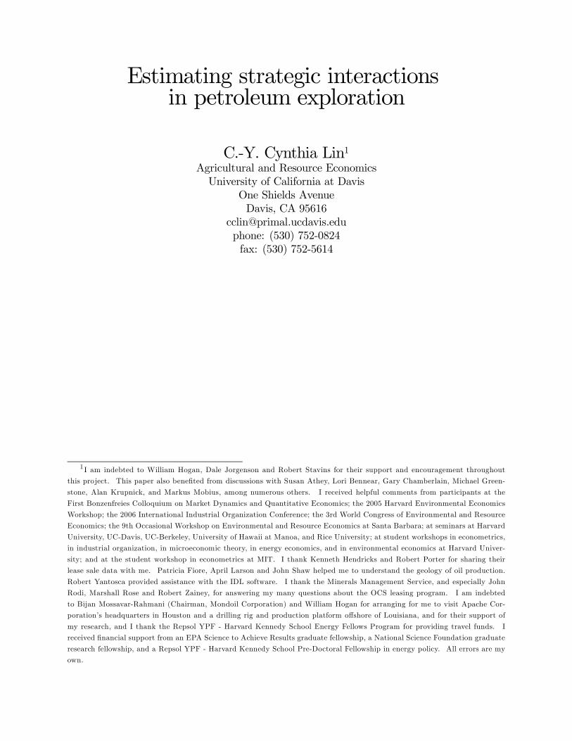
In total, there are 2404 tracts in my data set satisfying the above criteria, from 26
different lease sales. Table 1a presents summary statistics for these tracts; Figure 1 displays
the tract size distribution. The maximum tract size, as stipulated by a provision in section
8(b) of the Outer Continental Shelf Lands Act (OCSLA), 43 U.S.C. 1337(b)(1), is 5760 acres,
or 3 miles by 3 miles (Marshall Rose, Minerals Management Service, personal communication,
17 April 2003). Most tracts are either 2500 acres, 5000 acres or 5760 acres in size. The
average tract size is 4790 acres (s.d. = 1100) and the median tract size is 5000 acres. The
average real pre-sale value (in 1982 $) of these tracts, as estimated by the U.S. Department
of Interior Minerals Management Service, is $360 per acre, while the average winning bid is
$2520 per acre. Exploratory drilling eventually occurred on 1721 of the tracts. The U.S.
government divides the federal lands in the Gulf of Mexico offshore of Louisiana and Texas
into 51 areas; the data includes tracts from 26 of these areas.
For the panel data set, each time observation is a year.7 Tracts enter the panel when
they are sold. Tracts that were eventually explored exit the panel after the first drilling
occurs. Tracts that were never explored exit the panel after five years, which is the length
of the lease term a firm is given to begin exploration, or else relinquish its lease. Tracts have
5Another reason to focus on the earlier lease sales is that post-auction lease transfers occurred lessfrequently in the past (Porter, 1995; John Rodi, Minerals Management Service, personal communication, 8May 2003; Robert Porter, personal communication, 21 May 2003).
6It is possible for a lease to receive a suspension of production (SOP) or suspension of operations (SOO)which will extend the life of the lease beyond its primary term (Jane Johnson, Minerals Management Service,personal communication, October 29, 2003). Exploratory drilling first occurred after the lease term on 77(or 3.1 %) of the 2481 wildcat tracts sold before 1980.
7As a robustness check, I also repeat my analyses on a panel in which each time period is a quarter, or91 days.

C.-Y.C. Lin 12
on average 2.03 time observations in the panel. The panel spans the years 1954 to 1983.
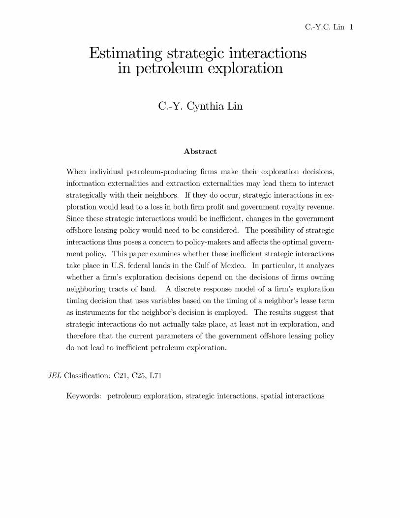
Figure 2 plots the aggregate hazard rate of exploration. The aggregate hazard rate Ht
at time t is computed as the number of tracts that explored at time t divided by the risk
set Rt at time t, where the risk set is simply the set of tracts that have not explored before
time t. Following Hendricks and Porter (1996), the standard deviation of the hazard ispHt (1−Ht) /Rt; the error bars in the figure indicate plus or minus one standard deviation.
The aggregate hazard rate exhibits a U-shaped pattern: the hazard rate of exploration is
monotonically decreasing with time except in the year right before the lease term expires,
when there is a spike in exploration. It is this U-shaped feature that I exploit to construct
my instruments for the neighbors’ exploration decision. Since the hazard rate of exploration
is high in both the first and last years of the lease term, my instruments for the fraction of
neighbors who explored at any time t are the fraction of neighbors in the first year of their
lease at time t and the fraction of neighbors in the last year of their lease term at time t.
Although the set of possible tracts i is limited to wildcat tracts sold before 1980 for which
exploration did not occur after the lease term, the set of possible neighbors for these tracts i
is larger. In particular, any tract sold between 1954 and 1983, inclusive, for which location
data is available, for which the first exploration did not occur before the sale date and for
which production did not occur before exploration is eligible as a potential neighbor for a
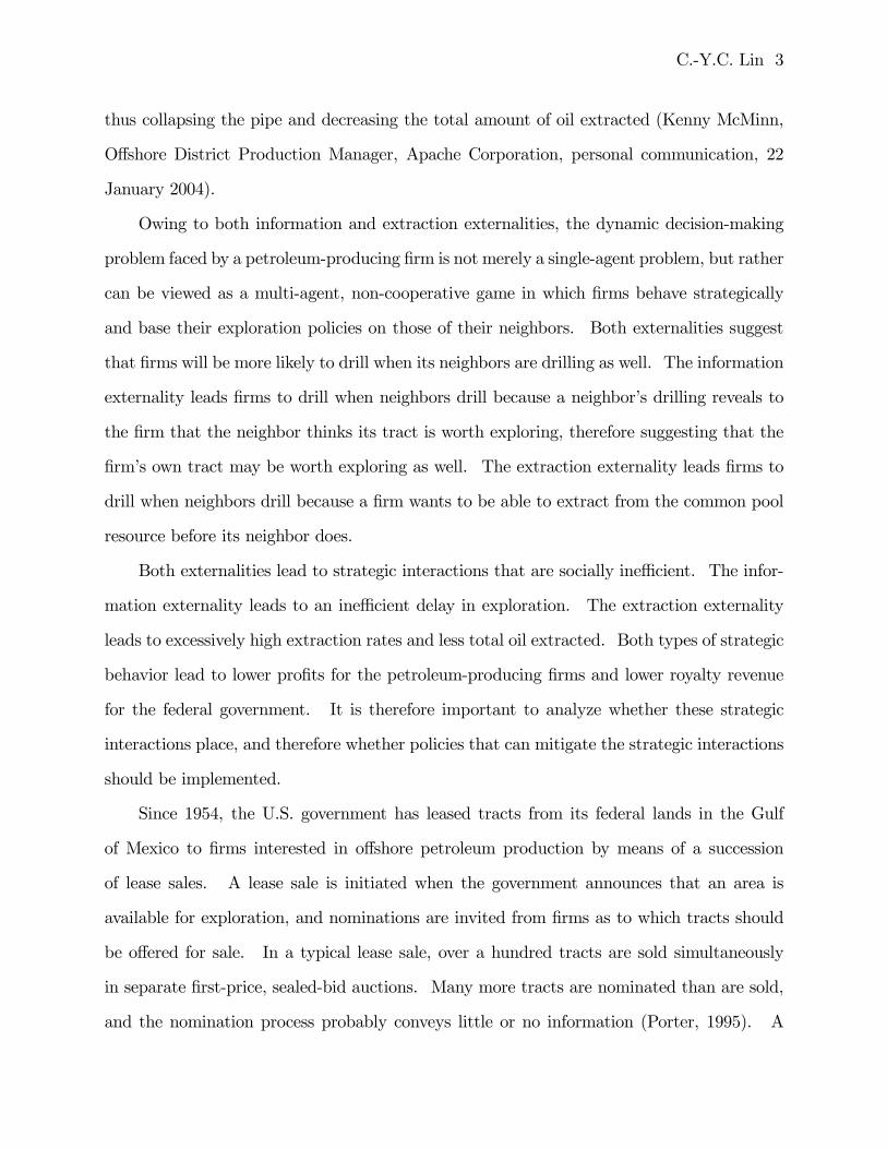
tract i. Figure 3 plots the location of each of the tracts used in my reduced-form analyses.8
Wildcat tracts i included in my sample are denoted with a filled circle. Other tracts that may
serve as potential neighbors to these tracts are denoted with an open diamond; these tracts
include drainage and developmental tracts sold between 1954 and 1983, inclusive, as well as
wildcat tracts that were sold between 1980 and 1983, inclusive, and wildcat tracts that began
exploration after the lease term. For a sense of the geographic span of a neighborhood, the
8I use the latitude-longitude coordinates provided by Hendricks and Porter. The longitude and latitudeare compiled from the well-bore tape as the average of the longitude (or latitude) over all wells recorded inthe block for the entire coverage period of the tape. The tape includes spud dates from January 13, 1947 toJuly 6, 1991. This is intended to give a ”representative location” of the tract. The location for blocks noton the well-bore tape was approximated by map inspection.

C.-Y.C. Lin 13
grey asterisk in Figure 3 denotes a wildcat tract and the circle around it encompasses all
tracts located within 5 miles from it.
To be considered an actual neighbor for a given tract i at time t, a potential neighbor
must also satisfy the conditions listed in the previous section: namely, that (i) it is located
within a certain distance of tract i, (ii) its lease began before time t, (iii) it has not been
explored before time t − 1, and (iv) it is owned by a different firm from the firm owning
tract i,9 and, in most cases, (v) all of tract i’s neighbors at time t must be sold on a different
date from tract i. In the base case, the distance used to define neighbors was 5 miles; for
robustness, the analyses were also run using 4 miles, 6 miles and 10 miles.
Table 1b presents the summary statistics for variables that varied over both tract and
time. Each column represents a different case. The base case is column (1). In the base
case, the time period is one year in length, neighbors are located within 5 miles, and the
additional restriction (v) that all of tract i’s neighbors at time t must be sold on a different
date from tract i is imposed. There are 1139 observations in the base case. For the other
cases, I vary the time period, the distance of the furthest neighbor, and whether or not all
neighbors have to be sold on a different sale date. In the base case, a tract has on average
1.74 (s.d. = 1.00) neighbors at any time t.10 Of its neighbors, on average 43% of them
began exploration in the previous period. Moreover, during the previous period an average
of 36% and 15% of a tract’s neighbors were in the first and last years of their lease term,
respectively.
9For cases in which multiple firms share the lease for a tract, I define the owner of the tract as the firmwith the highest share in the bid, as this firm is likely to have the primary decision-making authority.10The base case cutoff of 5 miles was chosen so that a neighborhood would be at least as large as the size of
most petroleum fields. To date, 79% and 70% of the fields spanned 3 or fewer leases for blocks with maximumwater depth of 0-199 meters and 200-399 meters, respectively (Marshall Rose, Minerals Management Service,personal communication, 31 March 2005).

C.-Y.C. Lin 14
4 Results
As a benchmark, Table 2 presents the results from running the discrete response models
without the use of instruments, when neighbors must be located within 5 miles of a tract.
In specifications (1) and (2), the linear probability model and the probit model, respectively,
are run with the base case sample in which the time period is one year in length, neighbors
are located within 5 miles, and the additional restriction (v) that all of tract i’s neighbors at
time t must be sold on a different date from tract i is imposed. For robustness, specification
(3) runs the linear probability model on the sample in which restriction (v) is relaxed; spec-
ification (4) runs the linear probability model on quarterly data. The coefficient of interest
is that on the fraction of neighbors who drilled at time t − 1. For all four specifications,
neighbors do not have a significant effect. However, the other covariates have coefficients of
the expected sign: the probability of exploring increases with the estimated pre-sale value,
the winning bid and the size (acreage) of the tract. Also as expected, the probability of
exploring often decreases with the number of years since the lease sale, with the coefficient
being either significantly negative or insignificant at a 5% level, and increases at the last
year of the lease term.
To test for the endogeneity of the neighbors’ drilling, a Durbin-Wu-Hausman test is
used for the linear probability model and a Smith-Blundell test is used for the probit model.
Both are tests of whether the residual from a regression of the variable in question on all the
exogenous variables has a significant coefficient when added to the original model; the table
reports the p-value from the tests under the null hypothesis that the variable is exogenous.
According to these tests, neighbors’ decisions are not significantly endogenous at a 5% level
in any of the four specifications. Although the tests fail to reject an exogeneity assumption,
it still seems plausible, at least in theory, that neighbors’ decisions are endogenous owing to
simultaneity and/or spatially correlated unobservables.
To guard against any potential endogeneity of the neighbors’ decisions, I instrument for
the fraction of neighbors who drill with the fraction of neighbors in the first year of the lease

C.-Y.C. Lin 15
and the fraction of neighbors at the last year of the lease term. Table 3 presents the results
from first-stage regression of the endogenous variable on the instruments and the covariates
for the base case (specification (1)), as well as for three variants. The first-stage F-statistic
from a joint test of the two instruments is over 10 in all specifications, so weak instruments
should not be a concern (Stock & Watson, 2003). The instruments are thus correlated with
the neighbors’ decisions.
Table 4a presents the results from running the discrete response analysis with the use of
instruments, when neighbors must be located within 5 miles of a tract. Irrespective of the
probability model (linear or probit), the time period (year or quarter) and whether or not
the restriction (v) that all of tract i’s neighbors at time t must be sold on a different date
from tract i is imposed, the effect of neighbors’ decisions is statistically insignificant and
small: according to the results from the base case specification (1), a change in the percent
of neighbors who explored in the previous period from 0 percent to 100 percent would only
increase a firm’s probability of exploration by a statistically insignificant 0.14. Negative
effects greater than 0.15 and positive effects greater than 0.43 on a firm’s probability of
exploration can be rejected at a 5% level.
As with the uninstrumented regressions, the signs of the coefficients on the other co-
variates are as expected. According to the results from the base case specification (1), an
increase in the real pre-sale value of a tract of $10,000 per acre would increase the probability
of exploration by 0.66. Thus, pre-sale values, which vary greatly from $0 to $18,230 per
acre, have a very large and statistically significant effect on exploration decisions. Similarly,
an increase in the winning bid of $10,000 per acre would increase the probability of explo-
ration by 0.34. Thus, winning bids, which vary from $450 to $60,800 per acre, have a large
and statistically significant effect as well. The coefficients on the pre-sale value and on the
winning bid indicate that, all else equal, tracts are more likely to be explored if their ex ante
estimated values are high.
The coefficient on acreage indicates that an increase in tract size of 100 acres increases
C.-Y.C. Lin 16
the probability of exploration by 0.40. Thus, larger tracts are more likely to be explored.
One likely explanation is that because larger tracts cover more surface area, the probability
that oil and gas reserves are present is higher.
The coefficient on the dummy for being in the last year of the lease term indicates that,
all else equal, a tract’s probability of being explored is higher by 0.13 when it is in the last
year of its lease term. This is because the option value to waiting goes to zero at the end
of the lease term.
In addition to being robust to the probability model, the time period and whether or
not the restriction (v) that all of tract i’s neighbors at time t must be sold on a different date
from tract i is imposed, the discrete response results are also robust to the distance used to
delineate neighbors; this can be readily seen in Table 4b, which compares the results from
using 5 miles as the cutoff in the base case to those from using 4 miles, 6 miles and 10 miles
in the linear probability model.
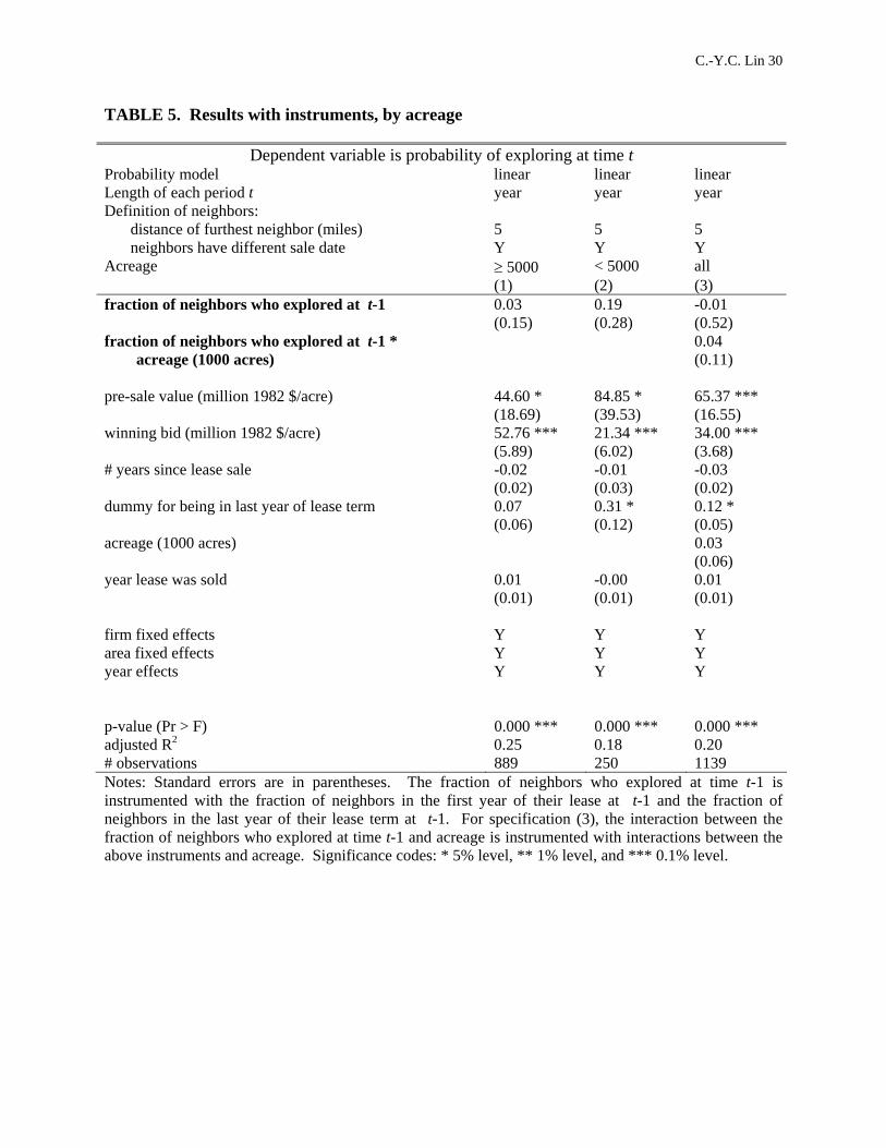
Externalities are likely to become more acute on smaller tracts, which are more likely to
be located over a common pool of oil reserve. To examine whether strategic interactions have
a larger effect on smaller tracts, where externalities arising from common-pool considerations
are likely to be more prevalent, the sample is also stratified by tract size (in acres). The
results are presented in Table 5. Specification (1) displays the results for larger tracts (i.e.,
tracts greater than or equal to 5000 acres in size); specification (2) displays the results for
smaller tracts (i.e., tracts less than 5000 acres in size). As the results indicate, neighbors
do not have a significant effect in either sample. Specification (3) includes a term that
interacts the fraction of neighbors who drilled at time t − 1 with the tract size, and is run
on all tract sizes.11 The coefficient on the fraction of neighbors who drilled at time t − 1
and the coefficient on the interaction term are both statistically insignificant. The result
that neighbors do not have a significant effect on a firm’s probability of exploratory drilling
is therefore robust to tract size.12
11This interaction term is instrumented with interactions between the original instruments and acreage.12Similar analyses were run using 2000 acres, 3000 acres and 4000 acres, respectively, as the cutoff between

C.-Y.C. Lin 17
Thus, regardless of whether instruments are used or not, the results of my discrete
response analysis do not indicate that a firm’s exploratory drilling decision depends on those
of its neighbors.13 Test results rejecting the endogeneity of neighbors’ decisions to a firm’s
own decision provide further evidence that neighbors do not base their decisions on each
other. My results are consistent with the weak results of Hendricks and Porter (1996): in
their regressions of the probability of initial exploration, the coefficients on the variables they
use to capture the neighborhood exploratory drilling experience are, for the most part, not
significant. Thus, even though one may expect information externalities to be particularly
acute on wildcat tracts, information and extraction externalities do not appear to induce
firms to interact strategically on net.
One possible explanation why the results reject strategic, non-cooperative behavior dur-
ing exploration is that firms owning neighboring tracts cooperate to jointly internalize the
inefficient externalities they impose on each other, for example by forming joint ventures
in exploration. Joint ventures in exploration occur less frequently than one might expect,
however, because negotiations are contentious, because firms fear allegations of pre-sale anti-
trust violations (Marshall Rose, Minerals Management Service, personal communication, 3
May 2005), and because prospective partners have an incentive to free ride on a firm’s in-
formation gathering expenditures (Hendricks and Porter, 1992). In their theoretical model
of the persuasion game, Hendricks and Kovenock (1989) find that, even with well-defined
property rights, bargaining does not eliminate all the inefficiencies of decentralized drilling
decisions. As a consequence, the information externality may not be fully internalized.
Following exploration, firms can cooperate by consolidating their production rights
through purchase or unitization. Under a unitization agreement, a single firm is desig-
nated as the unit operator to develop the entire reservoir, while the other firms share in the
large and small tracts. The result that the neighbors do not have an effect regardless of tract size is robustto the cutoff used to delineate tract size.13Results from a Cox proportional hazards model without instruments also do not indicate that firms
interact strategically with their neighbors. The development of an instrumental variables analog of the Coxmodel using nonlinear instrumental variables techniques will be the subject of future work.
C.-Y.C. Lin 18
profits according to negotiated formulas (Libecap & Smith, 1999b). Unitization may reduce
the extraction externality. There are many obstacles to consolidation, however, including
contentious negotiations, the need to determine relative or absolute tract values, informa-
tion costs, and oil migration problems (Libecap & Wiggins, 1984). In addition, another free
rider problem that impedes coordination is that firms may fear that if they reveal to other
firms their information or expertise, for example about how to interpret seismic data, then
they may lose their advantage in future auctions (Hendricks & Porter, 1996). Thus, despite
various means of coordination, firms may still behave strategically and non-cooperatively,
and information and extraction externalities may not be fully internalized.
A second, more likely, explanation why the results reject strategic, non-cooperative
behavior during exploration is that the externalities are insignificant or even nonexistent
during exploration, and do not become important until later stages of production. In
her structural econometric model of the multi-stage investment timing game in petroleum
production, Lin (2007) finds that while externalities from exploration have any net strategic
effect, externalities from subsequent development, during which firms install production
platforms, do have a net strategic effect. A firm’s profits increase when its neighbor installs
a production platform, perhaps because this is a signal to the firm that the neighbor’s
exploratory efforts were successful, and therefore that there may be deposits present.14 In
contrast, seeing a neighbor install a drilling rig may provide little additional information
about a firm’s own lease, since the drilling may or may not be successful. As a consequence,
the information externality may be insignificant during exploration. Similarly, the extraction
externality may not become important until firms are actually extracting oil and competing
for the same resource, and therefore may also be insignificant during exploration as well.
14The main reason the development decision is excluded from the reduced-form analysis is that, just asfor exploration, a neighbor’s development decision is potentially endogenous. Development is not subject toa lease term, however, and thus, unlike for exploration, the timing of the lease term could not be exploitedfor instruments. The design of suitable instruments for the development decisions of one’s neighbors will bethe subject of future work.

C.-Y.C. Lin 19
5 Conclusion
This paper examines whether strategic considerations arising from information and ex-
traction externalities are present during petroleum exploration. In particular, it analyzes
whether a firm’s exploration timing decision depends on the decisions of firms owning neigh-
boring tracts of land. A discrete response model of a firm’s exploration timing decision with
instruments for the decisions of its neighbors is employed.
Do the positive information externalities and negative extraction externalities have any
net strategic effect that may cause petroleum production to be inefficient? The results do not
indicate that externalities from exploration have any net strategic effect. A firm’s exploration
decision does not depend significantly on the exploration decisions of its neighbors. This is
true even on smaller tracts, where strategic interactions are more likely, since smaller tracts
are more likely to be located over a common pool of oil reserve. A firm’s exploration decision
instead depends on exogenous factors such as the estimated pre-sale value of the tract, the
tract’s winning bid in the lease sale, whether or not it is the last year of the lease term, and
tract size.
A likely explanation why the results reject strategic, non-cooperative behavior during
exploration is that the externalities are insignificant or even nonexistent during exploration,
and do not become important until later stages of production. Seeing a neighbor install
a drilling rig may provide little additional information about a firm’s own lease, since the
drilling may or may not be successful. As a consequence, the information externality may
be insignificant during exploration. Similarly, the extraction externality may not become
important until firms are actually extracting oil and competing for the same resource, and
therefore may also be insignificant during exploration as well.
If they did occur, strategic interactions in exploration would lead to a loss in both
firm profit and government royalty revenue. Since these strategic interactions would be
inefficient, changes in the government offshore leasing policy would need to be considered.
Possible changes include modifying the tract size, enacting policies to facilitate joint ventures

C.-Y.C. Lin 20
and cooperation, and selling non-contiguous tracts of land in the lease sales. The possibility
of strategic interactions thus poses a concern to policy-makers and affects the optimal gov-
ernment policy. However, the results of the paper suggest that strategic interactions do not
actually take place, at least not in exploration, and therefore that the current parameters of
the government offshore leasing policy do not lead to inefficient petroleum exploration.
References
[1] Hendricks K, Kovenock D. Asymmetric information, information externalities, and effi-
ciency: The case of oil exploration. RAND Journal of Economics 1989; 20(2); 164-182.
[2] Hendricks K, Porter R. Joint bidding in federal OCS auctions. American Economic
Review Papers and Proceedings 1992; 82(2); 506-511.
[3] Hendricks K, Porter R. Determinants of the timing and incidence of exploratory drilling
on offshore wildcat tracts. NBER Working Paper Series (Working Paper No. 4605).
Cambridge, MA; 1993.
[4] Hendricks K, Porter R. The timing and incidence of exploratory drilling on offshore
wildcat tracts. The American Economic Review 1996; 86(3); 388-407.
[5] Libecap G, Smith J. Regulatory remedies to the common pool: The limits to oil field
unitization. Working paper. University of Arizona and Southern Methodist University;
1999a.
[6] Libecap G, Smith J. The self-enforcing provisions of oil and gas unit operating agree-
ments: Theory and evidence. The Journal of Law, Economics, and Organizations 1999b;
15(2); 526-548.

C.-Y.C. Lin 21
[7] Libecap G, Wiggins S. Contractual responses to the common pool: Prorationing of
crude oil production. The American Economic Review 1984; 74(1); 87-98.
[8] Libecap G, Wiggins S. The influence of private contractual failure on regulation: The
case of oil field unitization. The Journal of Political Economy 1985; 93(4); 690-714.
[9] Lin C-YC. Do firms interact strategically?: A structural model of the multi-stage
investment timing game in offshore petroleum production. Working paper. University
of California at Davis; 2007.
[10] Manski C. Identification of endogenous social effects: The reflection problem. Review
of Economic Studies 1993; 60(3); 531-542.
[11] Manski C. Identification Problems in the Social Sciences. Harvard University Press:
Cambridge, MA; 1995.
[12] Newey W. Efficient estimation of limited dependent variable models with endogenous
explanatory variables. Journal of Econometrics 1987; 36; 231-250.
[13] Porter R. The role of information in U.S. offshore oil and gas lease auctions. Econo-
metrica 1995; 63(1); 1-27.
[14] Robalino J, Pfaff A. Contagious development: neighbors’ interactions in deforestation.
Working paper. Columbia University; 2005.
[15] Stock J, Watson M. Introduction to Econometrics. Addison-Wesley: Boston; 2003.

C.-Y.C. Lin 22
TABLE 1a. Summary statistics by tract Variable # obs mean s.d. min max pre-sale value (thousand 1982 $/acre) 2404 0.36 1.12 0.00 18.23 winning bid (thousand 1982 $/acre) 2404 2.52 4.92 0.45 60.80 acreage (1000 acres) 2404 4.79 1.10 0.05 5.76 number of time observations 2404 2.03 1.73 0 4 number of years to exploration, conditional on exploring 1721 1.24 1.42 0 4 Note: The sample consists of wildcat tracts sold before 1980 whose date of first drilling did not occur after the lease term.
FIGURE 1.
Note: The sample consists of wildcat tracts sold before 1980 whose date of first drilling did not occur after the lease term.

C.-Y.C. Lin 23
FIGURE 2.
Hazard rate for exploratory drilling
0.00
0.05
0.10
0.15
0.20
0.25
0.30
0.35
0 1 2 3 4
Year since lease sale
Haz
ard
rate
Notes: The sample consists of wildcat tracts sold before 1980 whose date of first drilling did not occur after the lease term. Error bars indicate plus or minus one standard deviation.

C.-Y.C. Lin 24
FIGURE 3.
Notes: Filled circles denote the tracts used in the sample: these are wildcat tracts sold before 1980 whose date of first drilling did not occur after the lease term. Open diamonds denote other tracts that may be included as potential neighbors of the tracts in the sample. The grey asterisk highlights one of the wildcat tracts in the sample and the circle around it encompasses all tracts located within 5 miles of it.

C.-Y.C. Lin 25
TABLE 1b. Summary statistics by tract-year
Summary statistics Length of each period t year year year year year quarter Definition of neighbors:
distance of furthest neighbor 5 5 4 6 10 5 neighbors have different sale date Y N Y Y Y Y
(1) (2) (3) (4) (5) (6) dummy for exploring at time t 0.21
(0.41) 0.23
(0.42) 0.20
(0.40) 0.22
(0.42) 0.26
(0.44) 0.01
(0.12) dummy for being in the last year of lease term at time t 0.16
(0.37) 0.13
(0.34) 0.17
(0.37) 0.16
(0.36) 0.13
(0.34) 0.12
(0.33) # neighbors at time t 1.74
(1.00) 2.41
(1.61) 1.50
(0.76) 2.03
(1.33) 3.58
(2.90) 2.67
(1.97) maximum # neighbors at time t 7 9 6 9 23 15 fraction of neighbors who explored at t-1 0.43
(0.44) 0.36
(0.39) 0.42
(0.45) 0.43
(0.42) 0.46
(0.38) 0.06
(0.19) fraction of neighbors in the first year of lease at t-1 0.36
(0.45) 0.42
(0.47) 0.37
(0.46) 0.35
(0.44) 0.34
(0.42) 0.04
(0.17) fraction of neighbors in the last year of lease term at t-1 0.15
(0.33) 0.13
(0.32) 0.13
(0.32) 0.14
(0.32) 0.12
(0.28) 0.04
(0.16) # observations 1139 3932 951 1345 1854 6013 Notes: The table reports the mean for the given variables. Standard errors are in parentheses. The maximum number of neighbors at time t is simply the maximum. The sample of tracts consists of wildcat tracts sold before 1980 whose date of first drilling did not occur after the lease term. A tract-year is included for a given definition of neighbors if the tract has at least one of the designated type of neighbor at time t.

C.-Y.C. Lin 26
TABLE 2. Results without instruments
Dependent variable is probability of exploring at time t Probability model linear probit linear linear Length of each period t year year year quarter Definition of neighbors:
distance of furthest neighbor (miles) 5 5 5 5 neighbors have different sale date Y Y N Y
(1) (2) (3) (4) fraction of neighbors who explored at t-1 0.03
(0.03) 0.02 (0.02)
0.01 (0.02)
-0.01 (0.01)
pre-sale value (million 1982 $/acre) 67.13 *** (16.00)
34.64 ** (12.12)
59.19 *** (12.33)
7.92 ** (2.63)
winning bid (million 1982 $/acre) 34.64 *** (3.57)
27.97 *** (3.95)
42.52 *** (2.70)
4.63 *** (0.52)
# years since lease sale -0.03 * (0.01)
0.00 (0.01)
-0.02 * (0.01)
0.00 (0.00)
dummy for being in last year of lease term 0.14 ** (0.05)
0.15 ** (0.06)
0.16 *** (0.03)
0.00 (0.01)
acreage (1000 acres) 0.04 *** (0.01)
0.03 ** (0.01)
0.05 *** (0.01)
0.008 *** (0.002)
year lease was sold 0.01 (0.01)
0.03 *** (0.00)
0.00 (0.00)
-0.00 (0.00)
firm fixed effects Y Y Y Y area fixed effects Y Y Y Y year effects Y Y Y Y p-value (Pr > F for linear; Pr > c2 for probit) 0.000 *** 0.000 *** 0.000 *** 0.000 *** adjusted R2 (linear model) or pseudo R2 (probit model) 0.22 0.31 0.16 0.04 # observations 1139 1139 3932 6013
Test of endogeneity of fraction of neighbors who explored at time t-1 p-value 0.452 0.292 0.729 0.567 Notes: Standard errors are in parentheses. The probit results are the change in probability for a unit change in each dependent variable; continuous variables are evaluated at their mean. To test for the endogeneity of fraction of neighbors who explored at time t-1, a Durbin-Wu-Hausman test is used for the linear probability model and a Smith-Blundell test is used for the probit model. Both are tests of whether the residual from a regression of the variable in question on all the exogenous variables has a significant coefficient when added to the original model; the table reports the p-value from the tests under the null hypothesis that the variable is exogenous. Significance codes: * 5% level, ** 1% level, and *** 0.1% level.

C.-Y.C. Lin 27
TABLE 3. Discrete response analysis: First-stage regressions
Dependent variable is fraction of neighbors who explored at time t-1 Length of each period t year year quarter year Definition of neighbors:
distance of furthest neighbor (miles) 5 5 5 10 neighbors have different sale date Y N Y Y
(1) (2) (3) (4) fraction of neighbors in the first year of lease at t-1 -0.20 ***
(0.03) -0.11 *** (0.02)
-0.11 *** (0.01)
-0.17 *** (0.02)
fraction of neighbors in the last year of lease term at t-1 -0.09 * (0.04)
-0.03 (0.03)
-0.03 * (0.01)
-0.14 *** (0.03)
pre-sale value (million 1982 $/acre) 2.15 (17.51)
13.64 (11.56)
-7.95 * (3.94)
0.56 (8.95)
winning bid (million 1982 $/acre) 4.46 (3.90)
3.31 (2.53)
2.84 *** (0.78)
0.09 (2.01)
# years since lease sale -0.034 * (0.015)
-0.05 *** (0.01)
-0.00 (0.00)
-0.00 (0.01)
dummy for being in last year of lease term 0.08 (0.05)
0.12 *** (0.03)
-0.02 (0.01)
-0.01 (0.04)
acreage (1000 acres) 0.00 (0.01)
0.02 *** (0.01)
-0.00 (0.00)
-0.00 (0.01)
year lease was sold 0.013 * (0.006)
0.01 ** (0.00)
0.00 (0.00)
0.01 ** (0.00)
firm fixed effects Y Y Y Y area fixed effects Y Y Y Y year effects Y Y Y Y p-value (Pr > F) 0.000 *** 0.000 *** 0.000 *** 0.000 *** adjusted R2 0.20 0.15 0.14 0.34 # observations 1139 3932 6013 1854
Results from joint test of instruments F-statistic 18.05 16.37 13.03 28.70 p-value (Pr > F) 0.000 *** 0.000 *** 0.000 *** 0.000 *** Notes: Standard errors are in parentheses. Significance codes: * 5% level, ** 1% level, and *** 0.1% level.

C.-Y.C. Lin 28
TABLE 4a. Results with instruments
Dependent variable is probability of exploring at time t Probability model linear probit linear linear Length of each period t year year year quarter Definition of neighbors:
distance of furthest neighbor (miles) 5 5 5 5 neighbors have different sale date Y Y N Y
(1) (2) (3) (4) fraction of neighbors who explored at t-1 0.14
(0.15) 0.19 (0.16)
-0.06 (0.19)
0.04 (0.09)
pre-sale value (million 1982 $/acre) 66.46 *** (16.15)
52.90 ** (19.08)
60.11 *** (12.64)
8.25 ** (2.69)
winning bid (million 1982 $/acre) 34.15 *** (3.65)
43.04 *** (4.92)
42.72 *** (2.77)
4.49 *** (0.58)
# years since lease sale -0.03 (0.01)
0.01 (0.02)
-0.02 * (0.01)
0.00 (0.00)
dummy for being in last year of lease term 0.13 * (0.05)
0.19 * (0.09)
0.16 *** (0.04)
0.01 (0.01)
acreage (1000 acres) 0.04 *** (0.01)
0.05 ** (0.02)
0.05 *** (0.01)
0.008 *** (0.002)
year lease was sold 0.01 (0.01)
0.04 *** (0.00)
0.01 (0.01)
-0.00 (0.00)
firm fixed effects Y Y Y Y area fixed effects Y Y Y Y year effects Y Y Y Y p-value (Pr > F for linear; Pr > c2 for probit) 0.000 *** 0.000 *** 0.000 *** 0.000 *** adjusted R2 (linear model) or pseudo R2 (probit model) 0.21 0.26 0.15 0.03 # observations 1139 1037 3932 6013 Notes: Standard errors are in parentheses. The fraction of neighbors who explored at time t-1 is instrumented with the fraction of neighbors in the first year of their lease at t-1 and the fraction of neighbors in the last year of their lease term at t-1. The probit results are the change in probability for a unit change in each dependent variable; continuous variables are evaluated at their mean. Significance codes: * 5% level, ** 1% level, and *** 0.1% level.

C.-Y.C. Lin 29
TABLE 4b. Results with instruments, varying distance of neighbors
Dependent variable is probability of exploring at time t Probability model linear linear linear linear Length of each period t year year year year Definition of neighbors:
distance of furthest neighbor (miles) 5 4 6 10 neighbors have different sale date Y Y Y Y
(1) (5) (6) (7) fraction of neighbors who explored at t-1 0.14
(0.15) 0.01 (0.16)
0.04 (0.16)
0.05 (0.16)
pre-sale value (million 1982 $/acre) 66.46 *** (16.15)
56.49 ** (18.12)
48.32 *** (13.52)
50.84 *** (11.04)
winning bid (million 1982 $/acre) 34.15 *** (3.65)
36.56 *** (4.27)
31.29 *** (3.06)
28.94 *** (2.48)
# years since lease sale -0.03 (0.01)
-0.03 (0.02)
-0.04 * (0.01)
-0.04 ** (0.01)
dummy for being in last year of lease term 0.13 * (0.05)
0.12 * (0.05)
0.14 ** (0.05)
0.14 ** (0.05)
acreage (1000 acres) 0.04 *** (0.01)
0.05 ** (0.01)
0.05 *** (0.01)
0.04 *** (0.01)
year lease was sold 0.01 (0.01)
0.01 (0.01)
(0.01) (0.01)
0.00 (0.00)
firm fixed effects Y Y Y Y area fixed effects Y Y Y Y year effects Y Y Y Y p-value (Pr > F) 0.000 *** 0.000 *** 0.000 *** 0.000 *** adjusted R2 0.21 0.21 0.23 0.23 # observations 1139 951 1345 1854 Notes: Standard errors are in parentheses. The fraction of neighbors who explored at time t-1 is instrumented with the fraction of neighbors in the first year of their lease at t-1 and the fraction of neighbors in the last year of their lease term at t-1. Significance codes: * 5% level, ** 1% level, and *** 0.1% level.
C.-Y.C. Lin 30
TABLE 5. Results with instruments, by acreage
Dependent variable is probability of exploring at time t Probability model linear linear linear Length of each period t year year year Definition of neighbors:
distance of furthest neighbor (miles) 5 5 5 neighbors have different sale date Y Y Y
Acreage ≥ 5000 < 5000 all (1) (2) (3) fraction of neighbors who explored at t-1 0.03
(0.15) 0.19 (0.28)
-0.01 (0.52)
fraction of neighbors who explored at t-1 * acreage (1000 acres)
0.04 (0.11)
pre-sale value (million 1982 $/acre) 44.60 * (18.69)
84.85 * (39.53)
65.37 *** (16.55)
winning bid (million 1982 $/acre) 52.76 *** (5.89)
21.34 *** (6.02)
34.00 *** (3.68)
# years since lease sale -0.02 (0.02)
-0.01 (0.03)
-0.03 (0.02)
dummy for being in last year of lease term 0.07 (0.06)
0.31 * (0.12)
0.12 * (0.05)
acreage (1000 acres) 0.03 (0.06)
year lease was sold 0.01 (0.01)
-0.00 (0.01)
0.01 (0.01)
firm fixed effects Y Y Y area fixed effects Y Y Y year effects Y Y Y p-value (Pr > F) 0.000 *** 0.000 *** 0.000 *** adjusted R2 0.25 0.18 0.20 # observations 889 250 1139 Notes: Standard errors are in parentheses. The fraction of neighbors who explored at time t-1 is instrumented with the fraction of neighbors in the first year of their lease at t-1 and the fraction of neighbors in the last year of their lease term at t-1. For specification (3), the interaction between the fraction of neighbors who explored at time t-1 and acreage is instrumented with interactions between the above instruments and acreage. Significance codes: * 5% level, ** 1% level, and *** 0.1% level.