January, 2005

Estimating Standard Errors in Finance Panel Data Sets:Comparing Approaches

Mitchell A. PetersenKellogg School of Management, Northwestern University

and NBER

Abstract

In both corporate finance and asset pricing empirical work, researchers are often confrontedwith panel data. In these data sets, the residuals may be correlated across firms and across time, andOLS standard errors can be biased. Historically, the two literatures have used different solutions tothis problem. Corporate finance has relied on Rogers standard errors, while asset pricing has usedthe Fama-MacBeth procedure to estimate standard errors. This paper will examine the differentmethods used in the literature and explain when the different methods yield the same (and correct)standard errors and when they diverge. The intent is to provide intuition as to why the differentapproaches sometimes give different answers and give researchers guidance for their use.

I thank the Financial Institutions and Markets Research Center at Northwestern University’s KelloggSchool for support. In writing this paper, I have benefitted greatly from discussions with KentDaniel, Mariassunta Giannetti, Toby Moskowitz, Joshua Rauh, Michael Roberts, Paola Sapienza,and Doug Staiger, as well as the comments of seminar participants at the Federal Reserve Bank ofChicago, Northwestern University, and the Universities of Chicago and Iowa. The researchassistance of Sungjoon Park is greatly appreciated.

1 I searched papers published in the Journal of Finance, the Journal of Financial Economics, and the Reviewof Financial Studies in the years 2001- 2004 for a description of how the coefficients and standard errors were estimatedin a panel data set. I included both standard linear regressions as well as non-linear estimation techniques such as logitsand tobits in my survey. Panel data sets are data sets where observations can be grouped into clusters (e.g. multipleobservations per firm, industry, year, or country). I included only papers which reported at least five observations ineach dimension (e.g. firms and years). Papers which did to report the method for estimating the standard errors, orreported correcting the standard errors only for heteroscedasticity (i.e. White standard errors which are not robust towithin cluster dependence), were coded as not having correcting the standard errors for within cluster dependence.

1

I) Introduction

It is well known that OLS standard errors are correct when the residuals are independent and

identically distributed. When the residuals are correlated across observations, OLS standard errors

can be biased and either over or underestimate the true variability of the coefficient estimates.

Although the use of panel data sets (e.g. data sets that contain observations on the same firm from

multiple years) is common, the way that researchers have addressed possible biases in the standard

errors varies widely. In recently published finance papers which include a regression on panel data,

forty-five percent of the papers did not report adjusting the standard errors for possible dependence

in the residuals.1 Among the remaining papers, approaches for estimating the coefficients and

standard errors in the presence of within cluster correlation varied. 31 percent of the papers included

dummy variables for each cluster (e.g. for each firm). 34 percent of the papers estimated both the

coefficients and the standard errors using the Fama-MacBeth procedure (Fama-MacBeth, 1973). The

remaining two methods used OLS (or an analogous method) to estimate the coefficients but reported

standard errors adjusted for correlation within a cluster. Seven percent of the papers adjusted the

standard errors using the Newey-West procedure (Newey and West, 1987) modified for use in a

panel data set, while 22 percent of the papers reported Rogers standard errors (Williams, 2000,

Rogers, 1993, Moulton, 1990, Moulton, 1986) which are White standard errors adjusted to account

for possible correlation within a cluster. These are also called clustered standard errors.

2

Although the literature has used a diversity of methods to estimate standard errors in panel

data sets, it has provided little guidance to researchers as to when a given method is appropriate.

Since the methods can sometimes produce different estimates it is important to understand how the

methods compare, when they will produce different estimates of the standard errors, and when they

differ how to choose among the estimates. This is the objective of the paper.

There are two general forms of dependence which are most common in finance applications.

They will serve as the basis for the analysis. The residuals of a regression can be cross sectionally

correlated (e.g. the observations of a firm in different years are correlated). I will call this a firm

effect. Alternatively, the residuals of a given year may be correlated across firms. I will call this a

time effect. I will simulate panel data set with both forms of dependence, first individually and then

jointly. With the simulated data, I can estimate the coefficients and standard errors using each of the

methods and compare their performance. Section II contains the standard error estimates in the

presence of a fixed firm effect. Both the OLS and the Fama-MacBeth standard errors are biased

downward and the magnitude of this bias is increasing in the magnitude of the firm effect. The

Rogers standard errors are unbiased as they account for the dependence created by the firm effect.

The Newey-West standard errors, as modified for panel data, are also biased but their bias is small.

In section III, the same analysis is conducted with a time effect instead of a firm effect. Since

Fama-MacBeth procedure is designed to address a time effect, not a firm effect, the Fama-MacBeth

standard errors are unbiased and the coefficient estimates are more efficient than the OLS estimates.

The intuition of these first two sections carries over to Section IV, were I simulate data with both

a firm and a time effect. Thus far, the firm effect has been specified as a constant effect (e.g. does

not decay over time). In practice, the firm effect in the residual may decay over time and so the

3

Yit ' Xit β % εit (1)

correlation between residuals declines as the time between them grows. In Section V, I simulate data

with a more general correlation structure. This not only allows me to compare OLS, clustered, and

Fama-MacBeth standard errors in a more general setting, it also allows me to access the relative

benefit of using fixed effects (firm dummies) to estimate the coefficients and whether this changes

the way we should estimate standard errors. Most papers do not report standard errors estimated by

multiple methods. Thus in Section VI, I apply the standard error estimation techniques to two real

data sets and compare their relative performance. This allows me to provide guidance as to which

technique should be used in actual situations. It allows me to show how difference in standard error

estimates (e.g. White versus Rogers standard error) can provide information about the deficiency

in our models and directions for improving them.

II) Estimating Standard Errors in the Presence of a Fixed Firm Effect.

A) Robust Standard Error Estimates.

To provide intuition on why the standard errors produced by OLS are incorrect and how

Rogers standard errors correct this problem, it will be helpful to briefly review the expression for

the variance of the estimated coefficients. The standard regression for a panel data set is:

where we have observations on firms (I) across years (t). X and ε are assumed to be independent of

each other and to have a zero mean. The zero mean is without loss of generality and allows us to

ignore the intercepts and calculate the variances as sums of the squares of the variable. The

estimated coefficient is:

2 The Rogers standard errors are robust to heteroscedasticity residuals. However, since this is not my focus,I will assume that the errors are homoscedastic in the equations and simulations. I will use White standard errors as mybaseline estimates when analyzing actual data in section VI.

4

β̂OLS '

jN

i'1j

T

t'1Xit Yit

jN

i'1j

T

t'1X 2

it

'

jN

i'1j

T

t'1Xit (Xit β % εit)

jN

i'1j

T

t'1X 2

it

' β %

jN

i'1j

T

t'1Xit εit

jN

i'1j

T

t'1X 2

it

(2)

Var [ β̂OLS & β ] ' E jN

i'1j

T

t'1Xit εit

2

jN

i'1j

T

t'1X 2

it

&2

' E jN

i'1j

T

t'1X 2

it ε2it j

N

i'1j

T

t'1X 2

it

&2

' NT σ2X σ2

ε ( NT σ2X )&2

'σ2ε

NT σ2X

(3)

and the estimated variance of the coefficient is:

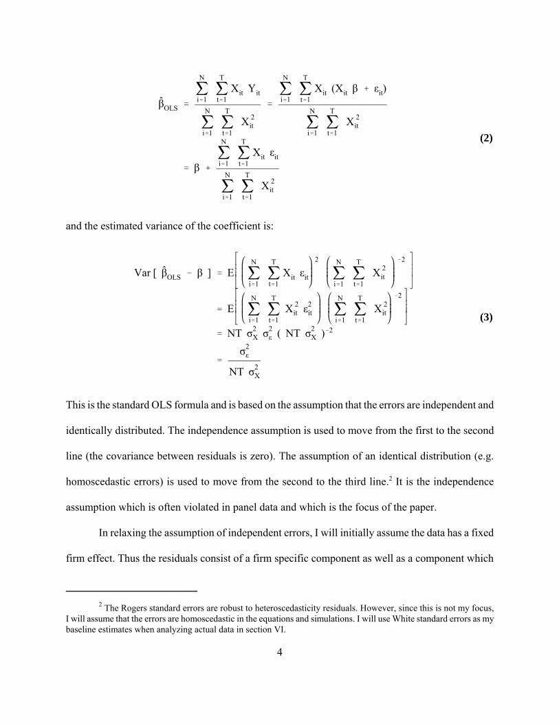
This is the standard OLS formula and is based on the assumption that the errors are independent and

identically distributed. The independence assumption is used to move from the first to the second

line (the covariance between residuals is zero). The assumption of an identical distribution (e.g.

homoscedastic errors) is used to move from the second to the third line.2 It is the independence

assumption which is often violated in panel data and which is the focus of the paper.

In relaxing the assumption of independent errors, I will initially assume the data has a fixed

firm effect. Thus the residuals consist of a firm specific component as well as a component which

3 Thus I am assuming that the model is correctly specified. I do this to focus on estimating the standard errors.In actual data sets, this assumption would need to be tested. Panel data sets often include a time effect as well as a firmeffect. For the moment, I assume there is no time effect and return to the implications of a time effect in Section III.

5

εit ' γi % ηit (4)

Xit ' µi % νit (5)

corr ( Xit , Xjs ) ' 1 for i' j and t ' s' ρX ' σ2

µ / σ2X for i' j and all t … s

' 0 for all i… jcorr ( εit , εjs ) ' 1 for i' j and t ' s

' ρε ' σ2γ / σ2

ε for i' j and all t … s' 0 for all i… j

(6)

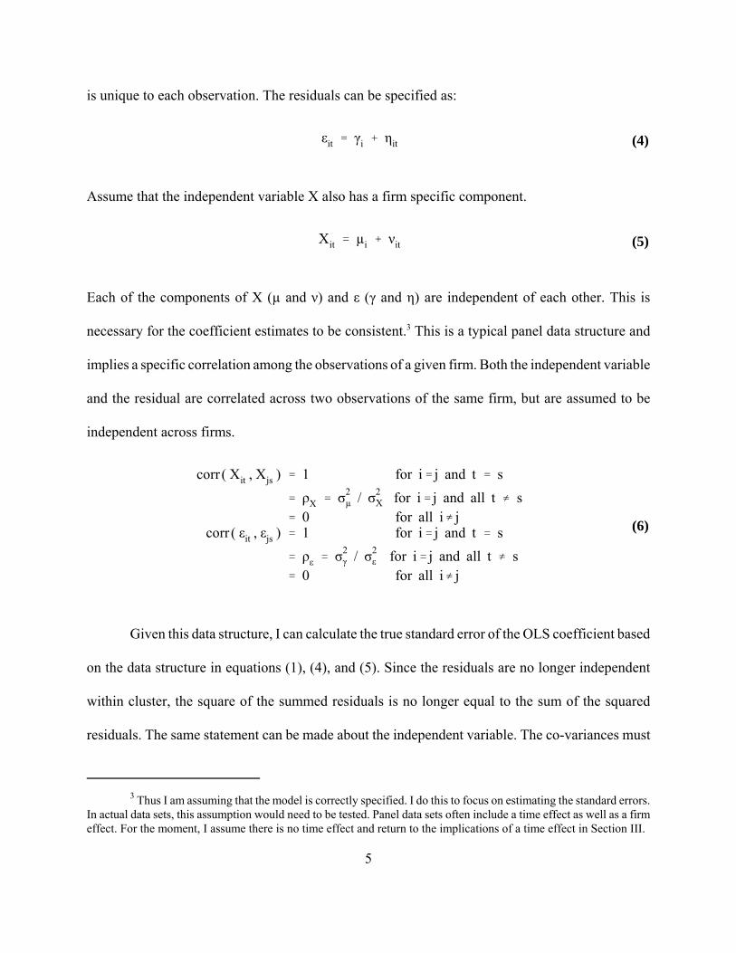
is unique to each observation. The residuals can be specified as:

Assume that the independent variable X also has a firm specific component.

Each of the components of X (µ and ν) and ε (γ and η) are independent of each other. This is

necessary for the coefficient estimates to be consistent.3 This is a typical panel data structure and

implies a specific correlation among the observations of a given firm. Both the independent variable

and the residual are correlated across two observations of the same firm, but are assumed to be

independent across firms.

Given this data structure, I can calculate the true standard error of the OLS coefficient based

on the data structure in equations (1), (4), and (5). Since the residuals are no longer independent

within cluster, the square of the summed residuals is no longer equal to the sum of the squared

residuals. The same statement can be made about the independent variable. The co-variances must

4 When calculating the square of the sum of X ε there are (NT)2 terms (see Figure 1). There are NT varianceterms [σ2(X) σ2(e)]. These are the only ones included in the OLS standard errors. There are NT(T-1) non-zero offdiagonal terms [(T(T-1) for each of N firms]. These are non-zero when there is a firm effect. The remaining NT2(N–1)diagonal terms are assumed to be zero. If there is a time effect, then NT(N–1) of these would be non-zero as well [N(N-1) for each of T years].

Var [ β̂OLS & β ] 'σ2ε

NT σ2X

1 %2T j

T

k'1(T&k) ρx,k ρε ,k

5 If the firm effect is not fixed, the correlation of εt and εs will be a non-trivial function of t-s. In this case, theequation will be a sum of all the correlations between εt and εt-k times the covariance between Xt and Xt-k. When thecorrelations are not constant, the variance of the coefficient estimate is:

When the auto-correlations are not constant, they can be negative or positive. Thus it is possible for the OLS standarderrors to under or over-estimate the true standard error. I will address auto-correlations which decay as the lag length(k) increases in Section V, when we examine non-fixed firm effects. Finally, if the panel is unbalanced, the true standarderror and the bias in the OLS standard errors will be even larger (Moulton, 1986).

6

Var [ β̂OLS & β ] ' E jN

i'1j

T

t'1Xit εit

2

jN

i'1j

T

t'1X 2

it

&2

' E jN

i'1j

T

t'1Xit εit

2

jN

i'1j

T

t'1X 2

it

&2

' E jN

i'1j

T

t'1X 2

it ε2it % 2 j

T&1

t'1j

T

s't%1Xit Xis εit εis j

N

i'1j

T

t'1X 2

it

&2

' N T σ2X σ2

e % N T (T&1) ρx σ2X ρe σ

2e NT σ2

X&2

'σ2ε

NT σ2X

1 % (T&1) ρX ρε

(7)

be included as well.4 The variance of the OLS coefficient estimate is now:

I used the assumption that residuals are independent across firms [e.g. I … j, see equation (6)]

in deriving the second line. Given the assumed data structure, the within cluster correlations of both

X and ε are positive and are equal to the fraction of the variance which is attributable to the fixed

firm effect. When the data has a fixed firm effect, the OLS standard errors will always understate

the true standard error if and only if both ρX or ρε are non-zero.5 The magnitude of the error is also

S 2 ( β ) '

N (NT & 1) jN

i'1j

T

t'1Xit εit

2

(NT & k) (N & 1) jN

i'tj

T

t'1X 2

it

6The exact formula for the Rogers standard error is:

7

increasing in the number of years in the data set (see Bertrand, Duflo, and Mullainathan, 2004). To

understand this intuition, consider the extreme case where the independent variables and residuals

are perfectly correlated across time (i.e. ρX =1 and ρε =1). In this case, each additional year provides

no additional information and will have no effect on the true standard error. However, the OLS

standard errors will assume each additional year provides N additional observations and the

estimated standard error will shrink accordingly and incorrectly.

The correlation of the residuals within cluster is the problem the Rogers standard errors

(White standard errors adjusted for clustering) are designed to correct.6 By squaring the sum of Xitεit

within each cluster, the covariance between residuals within cluster is estimated (see Figure 1). This

correlation can be of any form; no parametric structure is assumed. However, the squared sum of

Xitεit is assumed to have the same distribution across the clusters. Thus these standard errors are

consistent as the number of clusters grows (Donald and Lang, 2001; and Wooldridge, 2002). We

return to this issue in Section III.

B) Testing the Standard Error Estimates by Simulation.

To demonstrate the relative accuracy of the different standard error estimates and confirm

our intuition, I simulated a panel data set and then estimated the slope coefficient and its standard

error. By doing this multiple times we can observe the true standard error as well as the average

7 Each simulated data set contains 10 yearly observations on 500 firms, for a data set of 5,000 observations.The components of the independent variable and the residual are assumed to be normally distributed with zero means.For each data set, I estimated the coefficients and standard errors using each method described below. The reportedmeans and standard deviations reported in the tables are based on the 5,000 simulations.

8

estimated standard errors.7 In the first version of the simulation, I include a fixed firm effect but no

time effect in both the independent variable as well as in the residual. Thus the data was simulated

as described in equations (4) and (5). Across simulations I assumed that the standard deviation of

the independent variable and the residual were both constant at one and two respectively. This will

produce an R2 of 20 percent which is not unusual for empirical finance regressions. Across different

simulations, I altered the fraction of the variance in the independent variable which is due to the firm

effect. This fraction ranged from zero to seventy-five percent in twenty-five percent increments (see

Table 1). I did the same for the residual. This allows me to demonstrate how the magnitude of the

bias in the OLS standard errors varies with the strength of the firm effect in both the independent

variable and the residual.

The results of the simulations are reported in Table 1. The first two entries in each cell are

the average value of the slope coefficient and the standard deviation of the coefficient estimate. The

standard deviation is the true standard error of the coefficient and ideally the estimated standard

error will be close to this number. The average standard error estimated by OLS is the third entry

in each cell and is the same as the true standard error in the first row of the table. When there is no

firm effect in the residual (i.e. the residuals are independent across observations), the standard error

estimated by OLS is correct (see Table 1, row 1). When there is no firm effect in the independent

variable (i.e. the independent variable is independent across observations), the standard errors

estimated by OLS are also correct on average, even if the residuals are correlated (see Table 1,

column 1). This follows from the intuition in equation (7). The bias in the OLS standard errors is

8 In addition to a slope coefficient, all of the regressions also contained a constant whose true value is zero.The intuition from the slope coefficient results carry over to the intercept estimation. For example, when ρX = ρε = 0.50,the estimated slope coefficient averages -0.0003 with a standard deviation of 0.0669. The OLS standard errors are biaseddown (0.0283) and the Rogers standard errors are correct on average (0.0663).

The simulated residuals are homoscedastic, so calculating standard errors which are robust to heteroscedasticityis not necessary in this case. When I estimated White standard errors in the simulation they had the same bias as the OLSstandard errors. For example, the average White standard error was 0.0283 compared to the OLS estimate of 0.0283and a true standard error of 0.0508 (when ρX = ρε = 0.50).

9 The variability of the standard errors is small relative to their mean. For example, when ρX =ρε =0.50, themean OLS standard error is 0.283 with a standard deviation of 0.001 and the mean clustered standard error is 0.0508with a standard deviation of 0.003. Instead of reporting average standard errors, I could report the percent of t-statisticswhich are significant. Using the OLS standard error, 15.3 percent of the t-statistics are statistically significant at the onepercent level (i.e. the 99 percentile confidence interval contains the true coefficient 84.7 percent of the time). Using theclustered standard errors, 0.8 percent of the t-statistics are statistically significant at the one percent level. Since thestandard deviation of the standard error is usually small and the distribution symmetric, t-statistics, coverage percentagesand standard errors give the same intuition.

9

a product of the dependence in the independent variable (ρX) and the residual (ρε). When either

correlation is zero, OLS standard errors are unbiased.

When there is a firm effect in both the independent variable and the residual, then the OLS

standard errors underestimate the true standard errors, and the magnitude of the underestimation can

be large. For example, when fifty percent of the variability in both the residual and the independent

variable is due to the fixed firm effect (ρX = ρε = 0.50), the OLS estimated standard error is one half

of the true standard error (0.557 = 0.0283/0.0508).8 The standard errors estimated by OLS do not

change as I increase the firm effect across either the columns (i.e. in the independent variable) or

across the rows (i.e. in the residual). The true standard error does rise.

When I estimate the standard error of the coefficient using Rogers (clustered) standard errors,

the estimates are very close to the true standard error. These estimates rise along with the true

standard error as the fraction of variability arising from the firm effect increases. The Rogers robust

standard errors correctly account for the dependence in the data common in a panel data set (Rogers,

1993, Williams, 2000).9

10 There several differences between OLS and Fama-MacBeth estimates (Jagannathan, and Wang, 1998).Fama-MacBeth traditionally weights each year of data equally even if there is a different number of observations peryear. Thus in an unbalanced panel data set, the coefficient estimates can differ (Cohen, Gompers, and Vuolteenaho,2002, Vuolteenaho, 2002). Fama-MacBeth also runs cross sectional regressions, and thus any variable which does notvary across firms within a year (e.g. the stock market return) can not be estimated by the Fama-MacBeth method(Vuolteenaho, 2002, Cochrane, 2001). Since these have been dealt with elsewhere, I will not discuss them.

10

β̂FM ' jT

t'1

β̂t

T

'1T j

T

t'1

jN

i'tXit Yit

jN

i'tX 2

it

' β %1T j

T

t'1

jN

i'tXit εit

jN

i'tX 2

it

(8)

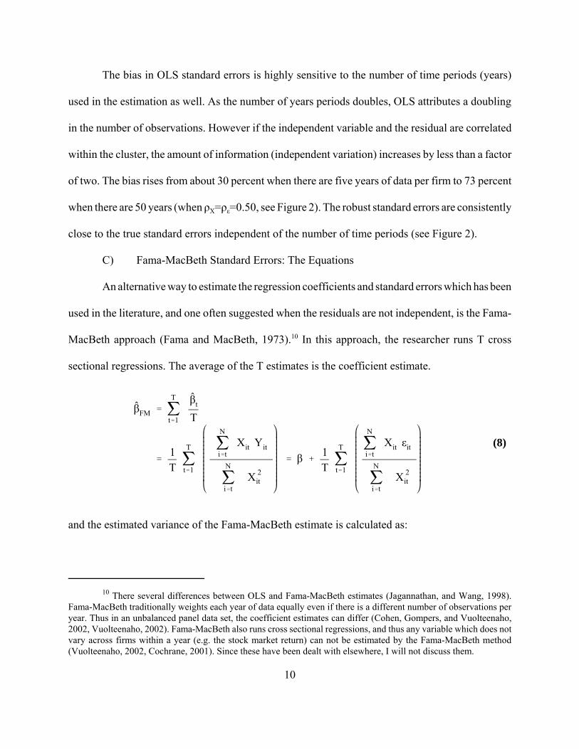
The bias in OLS standard errors is highly sensitive to the number of time periods (years)

used in the estimation as well. As the number of years periods doubles, OLS attributes a doubling

in the number of observations. However if the independent variable and the residual are correlated

within the cluster, the amount of information (independent variation) increases by less than a factor

of two. The bias rises from about 30 percent when there are five years of data per firm to 73 percent

when there are 50 years (when ρX=ρε=0.50, see Figure 2). The robust standard errors are consistently

close to the true standard errors independent of the number of time periods (see Figure 2).

C) Fama-MacBeth Standard Errors: The Equations

An alternative way to estimate the regression coefficients and standard errors which has been

used in the literature, and one often suggested when the residuals are not independent, is the Fama-

MacBeth approach (Fama and MacBeth, 1973).10 In this approach, the researcher runs T cross

sectional regressions. The average of the T estimates is the coefficient estimate.

and the estimated variance of the Fama-MacBeth estimate is calculated as:

11

S 2 ( β̂FM ) '1T j

T

t'1

( β̂t & β̂FM )2

T & 1(9)

Var( β̂FM ) '1

T 2Var( j

T

t'1β̂t )

'Var( β̂t )

T%

2 jT&1

t'1j

T

s't%1Cov( β̂t , β̂s )

T 2

'Var( β̂t )

T%

T (T&1)T 2

Cov( β̂t , β̂s )

(10)

Cov( β̂t , β̂s ) ' E jN

i'1X 2

it

&1

jN

i'1Xit εit j

N

i'1Xis εis j

N

i'1X 2

is

&1

' ( N σ2X )&2 E j

N

i'1Xit εit j

N

i'1Xis εis

' ( N σ2X )&2 E j

N

i'1Xit Xis εit εis

' ( N σ2X )&2 N ρX σ

2X ρε σ

2ε

'ρX ρε σε

N σ2X

(11)

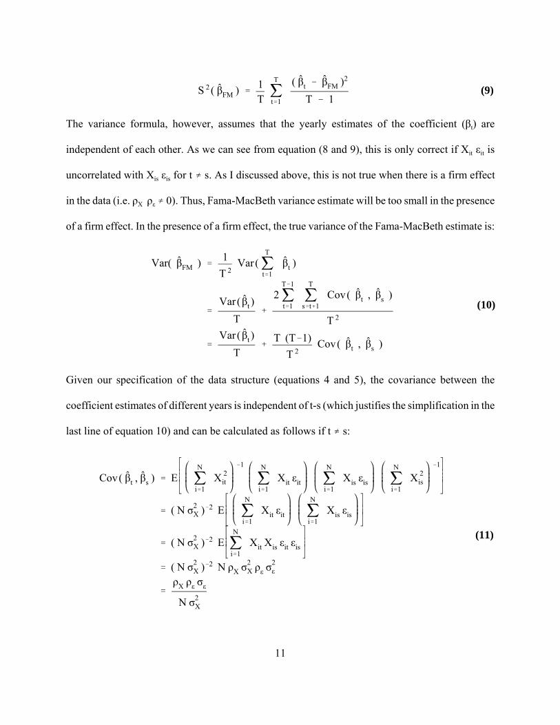
The variance formula, however, assumes that the yearly estimates of the coefficient (βt) are

independent of each other. As we can see from equation (8 and 9), this is only correct if Xit εit is

uncorrelated with Xis εis for t … s. As I discussed above, this is not true when there is a firm effect

in the data (i.e. ρX ρε … 0). Thus, Fama-MacBeth variance estimate will be too small in the presence

of a firm effect. In the presence of a firm effect, the true variance of the Fama-MacBeth estimate is:

Given our specification of the data structure (equations 4 and 5), the covariance between the

coefficient estimates of different years is independent of t-s (which justifies the simplification in the

last line of equation 10) and can be calculated as follows if t … s:

12

Var( β̂FM ) 'Var( β̂t )

T%

T (T&1)T 2

Cov( β̂t , β̂s )

'1T

σ2ε

N σ2X

%T (T&1)

T 2

ρX ρε σ2ε

N σ2X

'σ2ε

NT σ2X

1 % (T&1) ρX ρε

(12)

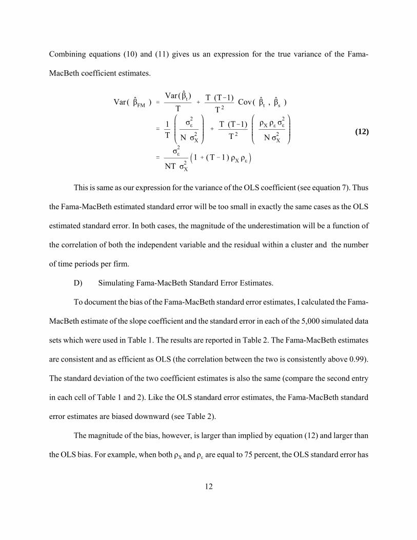
Combining equations (10) and (11) gives us an expression for the true variance of the Fama-

MacBeth coefficient estimates.

This is same as our expression for the variance of the OLS coefficient (see equation 7). Thus

the Fama-MacBeth estimated standard error will be too small in exactly the same cases as the OLS

estimated standard error. In both cases, the magnitude of the underestimation will be a function of

the correlation of both the independent variable and the residual within a cluster and the number

of time periods per firm.

D) Simulating Fama-MacBeth Standard Error Estimates.

To document the bias of the Fama-MacBeth standard error estimates, I calculated the Fama-

MacBeth estimate of the slope coefficient and the standard error in each of the 5,000 simulated data

sets which were used in Table 1. The results are reported in Table 2. The Fama-MacBeth estimates

are consistent and as efficient as OLS (the correlation between the two is consistently above 0.99).

The standard deviation of the two coefficient estimates is also the same (compare the second entry

in each cell of Table 1 and 2). Like the OLS standard error estimates, the Fama-MacBeth standard

error estimates are biased downward (see Table 2).

The magnitude of the bias, however, is larger than implied by equation (12) and larger than

the OLS bias. For example, when both ρX and ρε are equal to 75 percent, the OLS standard error has

13

Var[ βFM ] '1

T(T&1) jT

t'1

jN

i'tXit εit

jN

i'tX 2

it

&1T j

T

t'1

jN

i'tXit εit

jN

i'tX 2

it

2

'1

T(T&1) jT

t'1

jN

i't(µi%νit) (γi%ηit)

jN

i't(µi % νit)

2

&1T j

T

t'1

jN

i't(µi%νit) (γi%ηit)

jN

i't(µi % νit)

2

2 (13)

a bias of 60% (0.595 = 1 - 0.0283/0.0698, see Table I) and the Fama-MacBeth standard error has

a bias of 74 percent [ 0.738 = 1 - 0.0699/0.0183, see Table II ]. Moving down the diagonal of Table

2 from top left to bottom right, the true standard error increases but the standard error estimated by

Fama-MacBeth shrinks. As the firm effect becomes larger (ρX ρε increases), the bias in the OLS

standard error will grow, but the bias in the Fama-MacBeth standard error will grow even faster. The

incremental bias of the Fama-MacBeth standard errors is due to the way in which the estimated

variance is calculated. To see this we need to expand the expression of the estimated variance

(equation 9).

The true variance of the Fama-MacBeth coefficients is a measure of how far each yearly coefficient

estimate deviates from the true coefficient (one in our simulations). The estimated variance,

however, measures how far each yearly estimate deviates from the sample average. Since the firm

effect influences both the yearly coefficient estimates, and the average of the yearly coefficient

estimates, it does not appear in the estimated variance. Thus increases in the firm effect (increases

in ρXρε) will actually reduce the estimated Fama-MacBeth standard error at the same time it

increases the true standard error of the estimated coefficients. To make this concrete, take the

extreme example where ρXρε is equal to one. OLS will underestimate the standard errors by a factor

14

of %&&T (the standard error estimated by OLS is (σε/NTσX)½ while the true standard error is (σε/NσX)½.

The estimated Fama-MacBeth standard error will be zero. This additional source of bias will shrink

as the number of years increases since the estimate slope coefficient will converge to the true

coefficient (see Figure 2).

The firm effect may be less important in regressions where the dependent variable is returns

(and excess returns are serially uncorrelated) than in corporate finance applications where

unobserved firm effects can be very important (see Section VI). The biases which I have highlighted

will be less important in those applications. This isn’t surprising since the Fama-MacBeth technique

was developed to account for correlation between observations on different firms in the same year,

not to account for correlation between observations on the same firm in different years. In fact, Fama

and MacBeth (1973) examine the serial correlation of the residuals in their results and find that it

is close to zero. Its application in the literature, however, has not always been consistent with it

roots. Given the Fama-MacBeth approach was designed to deal with time effects in a panel data set,

not firm effects, I turn to this data structure in the next section.

E) Newey-West Standard Errors.

An alternative approach for addressing the correlation of errors across observation is the

Newey-West procedure (Newey and West, 1987). This procedure is traditionally used to account

for serial correlation of unknown form in the residuals of a single time series. It can be modified for

use in a panel data set by estimating only correlations between lagged residuals in the same cluster

(see Bertrand, Duflo, and Mullainathan, 2004, Doidge, 2004, MacKay, 2003, Brockman and Chung,

2001). The problem of choosing a lag length is simplified in a panel data set, since the maximum

11 In the standard application of Newey-West, a lag length of M implies that the correlation between εt and εt-kare included for k running from -M to M (excluding 0). When Newey-West has been applied to panel data sets,correlations between lagged and leaded values are only included when they are drawn from the same cluster. Thus acluster which contains T years of data per firm uses a maximum lag length (M) of T-1 and would include t-1 lags andT-t leads for the tth observation where t runs from 1 to T. Thus for the 4th year of data (t=4), we would include 3 lagsand 6 leads [ρ( εt εt-3 ) to ρ( εt εt-6)] when T=10.

15

lag length is one less than the maximum number of years per firm.11 To examine the relative

performance of the Newey-West and the robust/clustering approach to estimating standard errors,

I simulated 5,000 data sets with 5,000 observations each. Each data set includes 500 firms and ten

years of data per firm. The fixed firm effect was assumed to comprise twenty-five percent of the

variability of both the independent variable and the residual.

The standard error estimated by the Newey-West will be an increasing function of the lag

length in this simulation. When the lag length is set to zero, the estimated standard error is

numerically identical to the White standard error which is only robust to heteroscedasticity. This is

the same as the OLS standard error in my simulation, since the residuals are homoscedastic. Not

surprisingly, this estimate significantly underestimates the true standard error (see Figure 3). As the

lag length is increased from 0 to 9, the standard error estimated by the Newey-West rises from the

OLS/White estimate of 0.0283 to 0.0328 when the lag length is 9 (see Figure 3). In the presence of

a fixed firm effect, an observation of a given firm is correlated with all other observations for the

same firm no matter how far apart in time the observations are spaced. Thus having a lag length of

less than the maximum (T-1), will cause the Newey-West standard errors to underestimate the true

standard error when the firm effect is fixed (we return to temporary firm effects in Section V).

However, even with the maximum lag length of 9, the Newey-West estimates have a small bias –

underestimating the true standard error by 8% [0.084 = 1-0.0328/0.0358]. The robust standard errors

underestimate the true standard error by less than 2%.

16

jN

i'1j

T

t'1Xit εit

2

' jN

i'1j

T

t'1X 2

it ε2it % 2 j

T&1

t'1j

T

s't%1w( t&s ) Xit Xis εit εis

' jN

i'1j

T

t'1X 2

it ε2it % 2 j

T&1

t'1jT&t

j'1w( j ) Xit Xit&j εit εit&j

' jN

i'1j

T

t'1X 2

it ε2it % 2 j

T&1

t'1jT&t

j'11& j

TXit Xit&j εit εit&j

(14)

As the simulation demonstrates, the Newey-West approach to estimating standard errors, as

applied to panel data, does not yield the same estimates as the Rogers standard errors. The difference

between the two estimates is due to the weighting function used by Newey West. When estimating

the standard errors, Newey-West multiplies the covariance term of lag j (e.g. εt εt-j ) by the weight

[1-j/(M+1)], where M is the specified maximum lag. If I set the maximum lag equal to T-1, then the

central matrix in the variance equation of Newey-West is:

This is identical to the term in the Rogers standard error formula (see footnote 6) except for the

weighting function [w(j)]. The Rogers standard errors use a weighting function of one for all co-

variances. The Newey-West procedure was originally designed for a single time-series and the

weighting function was necessary to make the estimate of this matrix positive semi-definite. For

fixed j the weight w(j) approaches 1 as the maximum lag length (M) grows. Newey and West show

that if M is allowed to grow with the sample size (T), then their estimate is consistent. However, in

the panel data setting, the number of time periods is usually small. The consistency of the Rogers

standard error is based on the number of clusters (N) being large, opposed to the number of time

periods (T). Thus the Newey-West weighting function is unnecessary and leads to standard error

estimates which are slightly smaller than the truth in a panel data setting.

III) Estimating Standard Errors in the Presence of a Time Effect.

17

εit ' δt % ηitXit ' ζt % νit

(15)

To demonstrate how the two techniques work in the presence of a time effect I will generate

data sets which contain only a time effect (observations on different firms with in the same year are

correlated). This is the data structure for which the Fama-MacBeth approach was designed (see

Fama-MacBeth, 1973). If I assume that the panel data structure contains only a time effect, the

equations I derived above are essentially unchanged. The expressions for the standard errors in the

presence of only a time effect are correct once I exchange N and T.

A) Robust Standard Error Estimates.

Simulating the data with only a time effect means the dependent variable will still be

specified by equation (1), but now the error term and independent variable are specified as:

As before, I simulated 5,000 data sets of 5,000 observations each. I allowed the fraction of

variability in both the residual and the independent variable which is due to the time affect to range

from zero to seventy-five percent in twenty-five percent increments. The OLS coefficient, the true

standard error, as well as the OLS and robust standard error estimates are reported in Table 3. There

are several interesting findings to note. First, as with the firm effect results, the OLS standard errors

are correct when there is either no time effect in either the independent variable (σ(ζ)=0) or the

residual (σ(δ)=0). As the time effect in the independent variable and the residual rise, so does the

amount by which the OLS standard errors underestimate the true standard errors. When half of the

variability in both comes from the time effect, the OLS standard errors underestimate the true

standard errors by 91 percent [0.909 = 1 - 0.0282/0.3105, see Table 3].

The robust standard errors are much more accurate, but unlike our results with the firm

18

effects, they also underestimate the true standard error. The magnitude of the underestimate is small,

ranging from 13 percent [1-0.1297/0.1490] when the time effect comprises 25 percent of the

variability to 19 percent [1-0.3986/0.4927] when the time effect comprises 75 percent of the

variability. The problem arises due to the limited number of clusters (e.g. years). When I estimated

the standard errors in the presence of the firm effects, I had 500 firms (clusters) and ten years of data

per cluster. When I estimated the standard errors in the presence of a time effect, I have only 10

years (clusters) and 500 firms per year. Since the robust standard errors method places no restriction

on the correlation structure of the residuals with in a cluster, its consistency depends upon having

a sufficient number of clusters to estimate these standard errors. Based on these results, 10 clusters

is too small and 500 is sufficient (see Kezdi, 2002, and Bertrand, Duflo, and Mullainathan, 2004 for

similar results).

To explore this issue further, I simulated data sets of 5,000 observations but with the number

of years (or clusters) ranging from 10 to 100. In all of the simulations, 25 percent of the variability

in both the independent variable and the residual are due to the time effect [i.e. σ2(δ)/σ2(ε) =

σ2(ζ)/σ2(X) = 0.25]. The bias in the robust standard error estimates declines with the number of

clusters, dropping from 13 percent when there are 10 years (or clusters) to 4 percent when there are

40 years to under 1 percent when there are 100 years (see Figure 4). Thus, the bias in the robust

standard errors estimates is a product of the small number of clusters. However, since panel data sets

of 10 or 20 years are not uncommon in finance, this may be a problem in practice.

B) Fama-MacBeth Estimates

When there is only a time effect, the correlation of the estimated slope coefficients across

the years will be zero and the standard errors estimated by Fama-MacBeth will be correct (see

12 The robust (White or Rogers) approach to estimating standard errors changes only the estimated standarderrors. The coefficient estimates are numerically identical to OLS and thus have the same efficiency and variance asOLS.

19

equation 9 and 12). This is exactly what we find in the simulation (see Table 4). The estimated

standard errors are extremely close to the true standard errors and thus the confidence intervals will

be the correct size. In addition to producing unbiased standard error estimates, Fama-MacBeth also

produces more efficient estimates than OLS.12 For example, when 25 percent of the variability of

both the independent variable and the residual is due to the time effect, the standard deviation of the

Fama-MacBeth estimate is 81 percent [1-0.0284/0.1490] smaller than the standard error of the OLS

estimate (compare Table 3 and 4). The improvement in efficiency arises from the way in which

Fama-MacBeth accounts for the time effect. By running cross sectional regressions for each year,

the intercept absorbs, and is an estimate of, the time effect. Since the variability due to the time

effect is no longer in the residual, the residual variability in the Fama-MacBeth regressions is

significantly smaller than in the OLS regression. The lower residual variance leads to less variable

coefficient estimates and greater efficiency. I will revisit this issue in the next section when I

consider the presence of both a firm and a time effect.

According to the simulation results thus far, the best method for estimating the coefficient

and standard errors in a panel data set depends upon the source of the dependence in the data. If the

panel data only contains a firm effect, the Rogers standard errors (clustered by firm) are superior as

they produce standard errors which are correct on average. If the data has only a time effect, the

Fama-MacBeth estimates perform better than Rogers standard errors (clustered by time) when there

are few clusters (years). When the number of years is large, both the Rogers and Fama-MacBeth

standard errors are correct. The Fama-MacBeth estimates are more efficient than the OLS

13 It is possible to estimate robust standard errors accounting for clustering in multiple dimensions, but onlyif there are a sufficient number of observations within each cluster. For example, if a researcher has observations onfirms in industries across multiple years, she could cluster by industry and year (i.e. each cluster would be a specificyear and industry). In this case, since there are multiple firms in a given industry in each year, clustering would bepossible. If clustering was done by firm and year, since there is only one observation within each cluster, this isnumerically identical to OLS.

20

coefficients, although as we will see below this advantage disappears if time dummies are included.

IV) Estimating Standard Errors in the Presence of a Fixed Firm Effect and Time Effect.

Although the above results are instructive, they are unlikely to be completely descriptive of

actual data confronted by empirical financial researchers. Most panel data sets will likely include

both a firm effect and a time effect. Thus to provide guidance on which method to use I need to

assess their relative performance when both effects are present. In this section, I will simulate a data

set where both the independent variable and the residual have both a firm and a time effect.

The conceptual problem with using these techniques (Rogers or Fama-MacBeth standard

errors) is neither is designed to deal with correlation in two dimensions (e.g. across firms and across

time).13 The robust standard error approach allows us to be agnostic about the form of the correlation

with in a cluster. However, the cost of this is the residuals must be uncorrelated across clusters. Thus

if we cluster by firm, we must assume there is no correlation between residuals of different firms

in the same year. In practice, empirical researchers account for one dimension of the cross

observation correlation by including dummy variables and account for the other dimension by

clustering on that dimension. Since most panel data sets have more firms than years, the most

common approach is to include dummy variables for each year (to absorb the time effect) and then

cluster by firm (Anderson and Reeb, 2004, Gross and Souleles, 2004, Petersen and Faulkendar,

2004, Sapienza, 2004, and Lamont and Polk, 2001). I will use this approach in my simulations.

A) Rogers Standard Error Estimates.

21

To test the relative performance of the two methods, 5,000 data sets were simulated with

both a firm and a time effect. Across the simulations, the fixed firm effect comprises either 25 or 50

percent of the variability. The fraction of the variability due to the time effect is also assumed to be

25 or 50 percent of the total variability. This gives us three possible scenarios for the independent

variable [(25,25),(25,50), and (50,25)]. The scenario where fifty percent of the variability is due to

the firm effect and fifty percent is due to the time effect is excluded, as this would allow no

remaining variability in the firm-year specific component. The same three scenarios were used for

simulating the residual which generated nine different simulations (see Table 5).

The results in the presence of both a firm and time effect (Table 5) are qualitatively similar

to what we found in the presence of only a fixed firm effect (Table 1). The OLS standard errors

underestimate the true standard errors whereas the Rogers (clustered by firm) standard errors are

consistently accurate independent of how I specify the firm and time effects. As we saw above, the

bias in the OLS standard errors increases as the firm effect becomes larger. The magnitude of the

time effect does, however, appear to affect the magnitude of the bias in the OLS estimates, but this

effect is subtle. To see this intuition, it is useful to examine a couple of examples. In Table 1, when

the firm effect comprises 25 percent of the variability of both the independent variable and the

residual, OLS underestimated the standard error by 20 percent [1-0.0283/0.0353, see Table 1]. In

Table 5, there are two scenarios where the fixed firm effect is 25 percent for both the independent

variable and the residual. When the magnitude of the time effect rises to 25 percent, the bias in OLS

rises to 31 percent [1-0.0283/0.0407, see Table 5], and when the magnitude of the time effect rises

to50 percent, the bias in the OLS standard error is 45 percent [1-0.0283/0.0515, see Table 5]. The

time dummies, by absorbing the variability due to the time effect from the residual and the

14 The standard errors reported in Table 5 are very close to what is implied by the equations in Section II. OnceI adjust the definition of ρX and ρε to equal the fraction of variability due to the firm effect after removing the timeeffect, the OLS standard errors are very close to those produced by equation (3) and the Rogers standard errors are veryclose to those produced by equation (7).

22

independent variable, raise the fraction of the remaining variability which is due to the firm effect

(i.e ρX or ρε rise). This increases the bias in the OLS standard errors.14

B) Fama-MacBeth Estimates

The statistical properties of the OLS and Fama-MacBeth coefficient estimates are quite

similar. The means and the standard deviations of the estimates are almost identical (see Table 5 and

Table 6), and the correlation between the two estimates is never less than 0.999 in any of the

simulations. Once I include a set of time dummies in the OLS regression, which are effectively

included in the Fama-MacBeth estimates, the difference in efficiency I found in Tables 3 and 4

disappears. The OLS estimates are now as efficient as the Fama-MacBeth, even in the presence of

a time effect. However, the standard errors estimated by Fama-MacBeth are once again too small,

just as I found in the absence of a time effect (Table 2). As an example, when 25 percent of the

variability in both the independent variable and the residual comes from the firm effect and 25

percent comes from a time effect, the Fama-MacBeth standard errors underestimate the true standard

errors by 37 percent [1-0.0258/0.0407].

Most of the intuition from the earlier tables carry over. In the presence of a fixed firm effect

both OLS and Fama-MacBeth standard error estimates are biased down significantly. Rogers

standard errors which account for clustering by firm produce estimates which are correct on average.

The presence of a time effect, if it is controlled for with dummy variables, does not alter these

results, except for accentuating the magnitude of the firm effect and thus making the bias in the OLS

and Fama-MacBeth standard errors larger.

Var( ηit ) ' σ2ς if t ' 1

' φ2 σ2ς % (1 & φ2) σ2

ς ' σ2ς if t > 1

15 I multiply the ς term by %&1&- &φ&2 to make the residuals homoscedastic. From equation (16),

23

ηit ' ςit if t ' 1

' φ ηit&1 % 1 & φ2 ςit if t > 1(16)

V) Estimating Standard Errors in the Presence of a Temporary Firm Effect

The analysis thus far has assumed that the firm effect is fixed. Although this is common in

the literature, it may not always be accurate. The dependence between residuals may decay as the

time between them increases (i.e. ρ(εt , εt-k) may decline with k). In a panel with a short time series,

distinguishing between a permanent and a temporary firm effect may be impossible. However, as

the number of years in the panel increases it may be feasible to empirically identify the permanence

of the firm effect. In addition, if the performance of the different standard error estimators depends

upon the permanence of the firm effect, researchers need to know this.

A) Temporary Firm Effects: Specifying the Data Structure.

To explore the performance of the different standard error estimates in a more general

context, I simulated a data structure which includes both a permanent component (a fixed firm

effect) and a temporary component (non-fixed firm effect) which I assume is a first order auto

regressive process. This allows the firm effect to die away at a rate between a first order auto-

regressive decay and zero. To construct the data, I assumed that non-firm effect portion of the

residual (ηi t from equation 4) follows a first order auto regressive process:

Thus φ is the first order auto correlation between ηit and ηit-1, and the correlation between ηi t and ηi,t-k

is φk.15 Combining this term with the fixed firm effect (γi in equation 4), means the serial correlation

where the last step is by recursion (if it is true for t=k, it is true for t=k+1). Assuming homoscedastic residuals is notnecessary since the Rogers standard errors are robust to heteroscedasticity. However, assuming homoscedasticity makesthe interpretation of the results simpler. If I assume the residuals are homoscedastic, then any difference in the standarderrors I find is due to the dependence of observations within a cluster opposed to the presence of heteroscedasticity.

24

Corr (εi,t , εi,t&k ) 'Cov( γi % ηi,t ,γi % ηi,t&k )

Var ( γi % ηi,t ) Var ( γi % ηi,t&k )

'σ2γ % φk σ2

η

σ2γ % σ2

η

' ρε % (1 & ρε ) φk

(17)

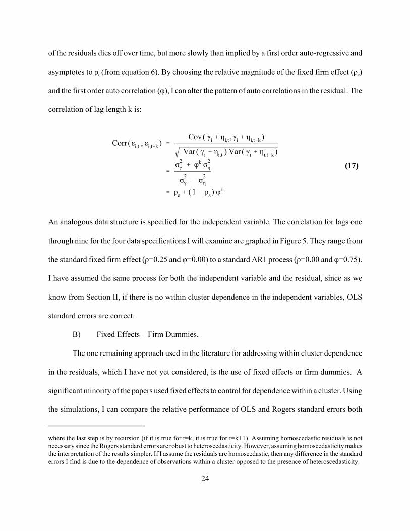
of the residuals dies off over time, but more slowly than implied by a first order auto-regressive and

asymptotes to ρε (from equation 6). By choosing the relative magnitude of the fixed firm effect (ρε)

and the first order auto correlation (φ), I can alter the pattern of auto correlations in the residual. The

correlation of lag length k is:

An analogous data structure is specified for the independent variable. The correlation for lags one

through nine for the four data specifications I will examine are graphed in Figure 5. They range from

the standard fixed firm effect (ρ=0.25 and φ=0.00) to a standard AR1 process (ρ=0.00 and φ=0.75).

I have assumed the same process for both the independent variable and the residual, since as we

know from Section II, if there is no within cluster dependence in the independent variables, OLS

standard errors are correct.

B) Fixed Effects – Firm Dummies.

The one remaining approach used in the literature for addressing within cluster dependence

in the residuals, which I have not yet considered, is the use of fixed effects or firm dummies. A

significant minority of the papers used fixed effects to control for dependence within a cluster. Using

the simulations, I can compare the relative performance of OLS and Rogers standard errors both

25

with and without firm dummies. The results are reported in Table 7, Panel A, column I.

The fixed effect estimates are more efficient in this case (0.0299 versus 0.0355). This is not

always true. The relative efficiency of the fixed effect estimates depends upon two offsetting effects.

Including the firm dummies uses up N–1 additional degrees of freedom and this raises the standard

deviation of the estimates. However, the firm dummies also eliminate the within cluster dependence

of the independent variable and the residual which reduces the standard deviation of the estimate.

In this example, the second effect dominates and thus the fixed effect estimates are more efficient.

Once we have included the firm effects, the OLS standard error are now correct and the

Rogers standard errors are not necessary (see Table 7 - Panel A, column I). The Rogers standard

errors are correct when we do not include the fixed effects and are slightly too large (5%) when we

include the fixed effects (see Kezdi (2002) for similar results). This conclusion, however, is sensitive

to the firm effect being fixed. If the firm effect decays over time, the firm dummies no longer

completely capture the within firm dependence and OLS standard errors are still biased. To show

this, I ran three additional simulations (see Table 7 - Panel A, columns II-IV). In these simulations,

the firm effect does decay over time (in column II, 92 percent of the firm effect dissipates after 9

years). Once the firm effect is temporary, the OLS standard errors again underestimate the true

standard errors even when firm dummies are included in the regression (Wooldridge, 2004, Baker,

Stein, and Wurgler, 2003). The magnitude of the underestimation depends upon the magnitude of

the temporary component of the firm effect (i.e. φ). The bias rises from about 17% when φ is 50

percent (column IV) to about 33 percent when φ is 75% (columns II and III). The Rogers standard

errors are much closer to the truth, but consistently over estimate the true standard error by about

5 percent across the simulations.

Variance correction ' 1 % 2 j10&1

k'1( 10 & k ) θk

16 Thus, instead of multiplying the variance by the infinite period adjustment [(1+θ)/(1-θ)], I multiplied it bythe 10 period adjustment

26

C) Adjusted Fama-MacBeth Standard Errors.

As noted above, the presence of a firm effect cause the Fama-MacBeth yearly coefficient

estimates to be correlated and this causes the Fama-MacBeth standard error to be biased downward.

A few authors who have used the Fama-MacBeth approach have acknowledged the bias and have

suggested adjusting the standard errors for the estimated first order auto-correlation of the estimated

slope coefficients (Chen, Hong, and Stein, 2001; Cochrane, 2001; Lakonishok, and Lee, 2001; Fama

and French, 2002; Bakshi, Kapadia, and Madan, 2003; Chakravarty, Gulen, and Mayhew, 2004).

The proposed adjustment is to estimate the correlation between the yearly coefficient estimates (i.e.

Corr[βt , βt-1 ] = θ), and then multiply the estimated variance by (1+ θ)/(1-θ) to account for serial

correlation of the βs (see Chakravarty, Gulen, Mayhew, 2004 and Fama and French, 2002, especially

footnote 1). This makes intuitive sense since the presence of a firm effect will cause the yearly

coefficient estimates to be serially correlated.

To test the merits of this idea, I simulated data sets where the fixed firm effect comprised 25

percent of the variance. For each simulated data set, ten slope coefficients were estimated, and the

auto correlation of the slope coefficients was calculated. I then calculated the original and adjusted

Fama-MacBeth standard errors, assuming both an infinite and a finite lag of T-1 periods (see

Lakonishok and Lee, 2001).16 The autocorrelation is estimated imprecisely as predicted by Fama and

French (2002). The 90th percentile confidence interval ranges from -0.60 to 0.41, but the mean is -

17 In the simulation the correlation between βt and βs ranged from 0.0430 to 0.0916 and did not decline as thedifference between t and s increased, since the firm effect is fixed. The theoretical value of the correlation between βtand βs should be 0.0625 (according to equation 11) and would imply a true standard error of the Fama-MacBeth estimateof 0.0354 (according to equation 12). This is what we found in Table II.

27

Cov( βt ,βt&1 ) ' E[ (βt & βTrue ) (βt&1 & βTrue ) ] (18)

0.1134 (see Table 7 - Panel B). Since the average first-order auto-correlation is negative, the

adjusted Fama-MacBeth standard errors are even smaller and more biased than the unadjusted

standard errors.

The intuition for why the proposed adjustment does not work is subtle. The problem is the

correlation which is being estimated (the within sample serial correlation of the yearly coefficient

estimates) is not the same as the one which is causing the bias in the standard errors (the population

auto-correlation of betas). The co-variance which biases the standard errors and which I estimate

across the 5,000 simulations is

To see how the presence of a fixed firm effect influences this covariance, consider the case where

the realization for firm i is a positive value of µiγi (i.e. the realized firm effect in both the

independent variable and the residual). This positive realization will result in an above average

estimate of the slope coefficient in year t, and because the firm effect is fixed it will also result in

an above average estimate of the slope coefficient in year t-1 (see equation 8). The realized value

of the firm effect (µi and γi) in a given simulation does not change the average β across samples. The

average β across samples is the true β or one in the simulations. Thus when I estimate the true

correlation between βt and βt-1, the firm effect causes this correlation to be positive and the Fama-

MacBeth standard errors to be biased downward.17

Researchers are given only one data set. Thus they must calculate the serial correlation of

18 The within sample serial correlation we estimate is actually less than zero, but this is due to a small samplebias. With only ten years of data per firm, I have only nine observations to estimate the serial correlation. To verify thatthis is correct, I re-ran the simulation using 20 years of data per firm and the average estimated serial correlation is closerto zero, rising from -0.1134 to -0.0556.

28

Cov( βt ,βt&1 ) ' E[ (βt & β̄Within sample ) (βt&1 & β̄Within sample ) ] (19)

the βs within the sample they are given. This co-variance is calculated as:

The within sample serial correlation measures the tendency of βt to be above its within sample mean

when βt-1 is above its within sample mean. To see how the presence of a fixed firm effect affects this

covariance, consider the same case as above. A positive realization of µiγi will raise the estimate of

β1 through βT, as well as the average of the βs (the Fama-MacBeth coefficient estimate) by the same

amount. Thus a fixed firm effect will no influence the deviation of any βt from the average β. Since

this deviation is the source of the estimated within sample serial correlation, we should expect that

the serial correlation calculated in sample would be zero on average.18 Since the within sample

correlation is asymptotically zero, adjusting the standard errors based on this estimated serial

correlation will still lead to biased standard error estimates.

The adjusted Fama-MacBeth standard errors do better when there is an auto-regressive

component in the residuals (i.e. φ > 0). In the three remaining simulations in Table 7 – Panel B, the

estimated within sample auto correlation is positive in all cases, but the adjusted Fama-MacBeth

standard errors are still biased downward. Adjusting the standard error estimates moves them closer

to the truth when the firm effect is not fixed (ρ=0). In this case, the standard errors based on the

infinite period adjustment underestimate the true standard error by 23 percent (1-0.0374/0.0484).

As the magnitude of the firm effect increases (compare columns II to III and IV), the bias in the

estimated standard errors increases. Thus the Fama-MacBeth standard errors adjusted for serial

29

correlation do better than the unadjusted standard errors when the firm effect decays over time, but

they still significantly underestimate the true standard errors.

VI) Empirical Applications.

The analysis thus far has been on simulated data. In these examples, I had the advantage of

knowing the data structure, which made choosing the method for estimating standard errors much

easier. In real world applications, we may have priors about the data’s structure (are firm effects or

time effects more important and are they permanent or temporary), but we do not know the data

structure for certain. Thus in this section, I will apply the different techniques for estimating

standard errors to two real data sets. This way I can demonstrate how the different methods for

estimating standard errors compare and also show what we can learn from the comparison.

For both data sets, I will first estimate the regression using OLS, and report White standard

errors as well as Rogers standard errors clustered by firm or year (Tables 8 and 9, columns I-III).

By using White standard errors as my comparison, difference across columns are attributable only

to within cluster correlations, but not to heteroscedasticity. If the Rogers standard errors clustered

by firm are dramatically different than the White standard errors, then we know there is a significant

firm effect in the data [e.g. Corr( Xi t εi t , Xi t-k εi t-k ) …0]. I then estimate the slope coefficients and

the standard errors using the Fama-MacBeth approach (Tables 8 and 9, columns IV-V). Finally, I

re-estimate OLS regression including firm dummies and report the slope coefficients and standard

errors clustered by firm and time (Table 8 and 9, columns VI-VIII). Each of the OLS regressions

include time dummies. This makes the efficiency of the OLS and Fama-MacBeth coefficients

similar, since as we discussed above, allowing the intercept to vary across years in the Fama-

19 The reported R2s do not include the explanatory power attributable to the time dummies. This is done tomake the R2 comparable between the OLS and the Fama-MacBeth results. Although the Fama-MacBeth procedureestimates a separate intercept for each year, the constant is calculated as the average of the yearly intercepts. Thus theFama-MacBeth R2 does not include the explanatory power of time dummies. Procedurally, I subtracted the yearly meansoff of each variable before running the OLS regressions.

30

MacBeth is similar to including time dummies in an OLS regression.19

A) Asset Pricing Application.

For the asset pricing example, I used the equity return regressions from Daniel and Titman

(2004, “Market Reactions to Tangible and Intangible Information”). They regress monthly equity

returns on annual values of lagged book to market ratios, historic changes in book and market

values, and a measure of the firm’s equity issuance. The details of the data set are briefly described

in the appendix and in more detail in their paper. Their method of constructing the data will induce

a large auto-correlation in the independent variables. Each observation of the dependent variable is

a monthly equity return. However, the independent variables are annual values (based on the prior

year). Thus for the twelve observations in a year, the dependent variable (equity returns) changes

each month, but the independent variable (e.g. past book value) does not.

To determine the importance of the firm or time effect in the data, I compared the White

standard errors to the Rogers standard errors (Table 8, column I vs. II). The Rogers standard errors

are essentially the same when I cluster by firm (ranging from three percent larger to one percent

smaller). This occurs because the auto-correlation in the residuals is effectively zero (see Figure 6).

The auto-correlation in the independent variable is large and persistent, starting at 0.98 the first

month and declining to 0.49 to 0.75 by the 24th month depending upon the independent variable.

However, since the adjustment in the standard error is a function of the auto-correlation in the Xs

(a large number) multiplied by the auto-correlation in the residuals (zero), the Rogers standard errors

31

clustered by firm are the same as the White standard errors.

The story is very different when I clustered by time (months). The standard errors clustered

by month are two to four times larger than the White standard errors. For example, the t-statistic on

the lagged book to market ratio is 7.2 if we use the White standard error and 1.9 if we cluster by

month. This means there is a significant time effect in the data (see Figure 7). Remember, however,

that the regression already contains time dummies. So any fixed time effect (i.e. one which raises

the monthly return by the same amount for every firm in a given month) has already been removed

from the data and will thus not affect the standard errors. Thus, the remaining correlation in the time

dimension must vary across observations (i.e. Corr[ ε i t ε j t ] varies across i and j).

Understanding a temporary firm effect is straightforward. The firm effect dies off over time

(is temporary) if the 1980 residual for firm A is more highly correlated to the 1981 residual for firm

A than to the 1990 residual. This is how I simulated the data in Section V (see Table 7). Visualizing

a non-constant time effect is more difficult. For the time effect to be temporary, it must be that a

shock in 1980 has a large effect on firm A and B, but has a significantly smaller affect on firm Z.

If the time effect influenced each firm in a given year by the same amount, the time dummies would

absorb the effect and clustering by time would not change the reported standard errors. The fact that

clustering by time does change the standard errors, means there must be a temporary time effect in

the data.

If we know the data, we can use our economic intuition to determine how the data should

be organized and predict the source of the dependence within a cluster. For example, since this data

set contains monthly equity returns we might consider how a shocks to the market would affect firms

differently. If the economy booms in a given month, firms in the durable goods industry may rise

20 A random coefficient model can generate a temporary time effect. For example, if the firm’s return dependsupon the firm’s β times the market return, but only the market return (or time dummies) are included in the regression,then the residual will contain the term { [ βi -Average(βi)] Market return t }. In this case, firms which have similar βswill have correlated residuals within a month, and firms which have very different βs will have residuals whosecorrelation is small. This is a temporary time effect. This logic suggests that I should instead sort by month, β, and thenfirm. When I sort this way, the auto-correlations are smaller and die away more slowly (declining from 0.030 at a lagof one to 0.028 at a lag of 24) than when I sorted by month, four-digit industry and firm (declining from 0.096 at a lagof one to 0.042 at a lag of 24).

32

more than firms in the non-durable goods industry. This can create a situation where the residuals

of firms in the same industry (in a month) are correlated with each other but less correlated with

firms in another industry (in that month). When I sort the data by month, four-digit industry, and

then by firm, I see evidence of this in the auto-correlation for the residuals and the independent

variables within each month. The results are graphed in Figure 7. The auto-correlations of the

residual is much larger than when I sorted by firm then month (compare Figure 6 and 7) and they

die away as we consider firms in more distant industries.20

When calculating the Rogers standard errors clustered by time, we don’t need to make an

assumption about how to sort the data. However, if researchers are going to understand what the

standard errors are telling us about the structure of the data, they need to consider the source of the

dependence in the residuals. By examining the different in the standard errors with no clustering,

when clustered by firm, and when clustered by time, we can determine the nature of the dependence

which remains in the residuals and this can guide us on how to improve our models.

According to the results in Sections II and III, the Fama-MacBeth standard errors perform

better in the presence of a time effect than a firm effect, and so given the above results should do

well in this data set. The Fama-MacBeth coefficients and standard errors are reported in column IV.

These results are a replica of those reported by Daniel and Titman (see Table 3, row 8 of their

paper). The coefficient estimates are similar to the OLS coefficients, and the standard errors are

33

much larger than the White standard errors (2 to 3.4 times) as we would expect in the presence of

a time effect. The Fama-MacBeth standard errors are close to the Rogers standard errors when we

cluster by time, as both methods are designed to account for dependence in the time dimension. The

Fama-MacBeth standard errors are consistently smaller than the Rogers standard errors, but the

magnitude of the difference is not large (twelve to eighteen percent, compare columns III and IV of

Table 8).

Cross-sectional, time-series regressions on panel data sets treat each observation equally. In

the Fama-MacBeth procedure, the monthly coefficient estimates are averaged using equal weights

for each month, but not each observation. Thus in an unbalanced panel, Fama-MacBeth effectively

weights each observation proportional to 1/Nt where Nt is the number of firms in month t. Since the

number of firms in this sample grows from about 1,000 per month at the beginning to almost 2,300

near the end of the sample, Fama-MacBeth will effectively under weight the later observations. To

correct this, I took a weighted average of the monthly coefficient estimates where the weights were

proportional to Nt. When I compare the weighted and un-weighted coefficient estimates and standard

errors, they are very close (compare columns IV and V of Table 8). In this case, the weights are

uncorrelated with the variables and thus do not effect the results.

The final set of regressions are OLS regression with both month and firm dummies included

(i.e. within estimates). I estimated White standard errors as well as Rogers standard errors clustered

by firm or month. The lesson from these results is the same as before. Clustering by firm does not

change the standard errors, but clustering by month leads to a significant, although smaller, increase

21 The coefficients change significantly when I include the firm dummies. For example, the coefficient on thelog(share issuance) falls by forty percent. Thus variation in a firm’s share issuance in a given year relative to the firm’saverage share issuance (which is what the within coefficient of -0.29 is measuring) has a smaller effect on returns thandifferences in average share issuance across firms (which is what the between coefficient of -0.97 is measuring(regression not reported) see Wooldridge, Chapter 10, 2002).

22 The White standard errors are still biased downward when I include firm dummies, but the magnitude ofthe bias is significantly smaller (compare columns VI and VII).

34

in the standard errors (52 to 229 percent larger).21

B) Corporate Finance Application.

For the corporate finance illustration, I used a capital structure regression. The independent

variables are those which are common from the literature (firm size, firm age, asset tangibility, and

firm profitability). I lagged the independent variables one year relative to the dependent variable,

used a long sample (1965-2003), and excluded firms which did not pay a dividend as in Fama and

French (2002). Table 9 contains both the OLS and Fama-MacBeth estimation results.

The relative importance of the firm effect and the time effect can be seen by comparing the

standard errors across the first three columns. The Rogers standard errors when I cluster by firm are

dramatically larger than the White standard errors (181-232 percent, see columns I and II).22 For

example, the t-statistic on the advertising to sales ratio is -1.9 when I use the White standard errors

and -0.7 when I use the Rogers standard errors clustered by firm. It is not surprising that R&D

expenditure is highly persistent, and thus the auto-correlation for R&D expenditure is extremely

high and persistent (see Figure 8). However, the auto-correlation in the residuals is also high and

even after 12 years the auto-correlation is still over 40 percent.

The importance of the time effect (after including time dummies) is generally much smaller

in this data set than in the previous one. The Roger’s standard errors clustered by time are generally

larger than the White standard errors but the magnitude of the difference is not big (except for the

35

market to book ratio). This is due to a smaller auto-correlation in the residuals (see Figure 9). When

I sorted by year, industry, and then firm, the residual first-order auto-correlation is less than 12

percent. The market to book standard error is the only one to increase dramatically and this occurs

because of the large temporary time effect we discussed in above.

These results also point out that the adjustment in the standard error can differ across

variables in both sign and magnitude. Relative to the Roger’s standard errors clustered by year, the

White standard errors overstate the standard error on the “R&D is positive” dummy by 12 percent

and understate the standard error on the market to book ratio by 64%. As long as the auto-correlation

in the residuals is zero, then the White standard errors are correct. However, when the auto-

correlation in the residuals is not zero (positive or negative), the bias in the standard errors will

depend upon how the time pattern of the residuals auto-correlation interacts with the time pattern

of the independent variable auto-correlations (see footnote 5).

The Fama-MacBeth standard errors provide the same intuition as the Rogers standard errors

clustered by time. In most cases, the Fama-MacBeth standard errors are quite close to the Rogers

standard errors clustered by year and close to the White standard errors. Since dependence in the

residual arises mostly from the firm effect, not the time effect, the bias in the Fama-MacBeth

standard errors is similar to the bias in the OLS standard errors (compare equations 7 and 12). The

only place where the standard error estimates differ is the advertising to sale ratio. The standard

error on the advertising to sales ratio is not directly comparable since the coefficient is not stable

across models. The coefficient ranges from -0.0977 when estimated by OLS to 0.0747 when

estimated by Fama-MacBeth. The weighted Fama-MacBeth estimate is -0.0002. The instability is

consistent with the imprecision of our estimate. Remember, when we corrected the standard errors

36

for a firm effect, the advertising to sales coefficient is no longer statistically different from zero.

VII) Conclusions.

It is well known from first-year econometrics classes that OLS standard errors are biased

when the residuals are not independent. How financial researchers should estimate standard errors

when using panel data sets has been less clear. The empirical literature has proposed and used a

variety of methods for estimating standard errors when the residuals are correlated across firms or

years in the data. In this paper, I find that the performance of the different methods varies and their

relative accuracy depends upon the nature of the within cluster dependence.

Since Fama-MacBeth estimation was designed for a setting where residuals were correlated

within a year, but not across firms, it does well in this context. It produces estimates which are more

efficient than OLS estimates (although this is easily fixed with time dummies) and standard errors

which are as good as Rogers standard errors (clustered by time) when the number of clusters is large,

and better when the number of clusters is small.

The Rogers standard errors (clustered by firm) are more accurate in the presence of a firm

effect than standard errors estimated by OLS, Fama-MacBeth, Fama-MacBeth corrected for first-

order auto-correlation, or Newey-West (modified for panel data sets). In addition, the Rogers

standard errors are robust to different specifications of the dependence (permanent or temporary

effects). The Rogers estimates produce correct standard errors and correctly sized confidence

intervals in the presence of a firm or time effects, whether the effect is permanent or temporary when

clustered on the same dimension (firm or time). It is only in the case there the firm effect is

temporary, that the Rogers standard errors are superior to a fixed effect model. Since the precise

form of the dependence in the residual and the independent variables is often unknown, an estimate

37

which is robust to different specifications is an advantage.

Finally, the result of the simulations, and more importantly the results from the two

applications, point out the diagnostic value of estimating standard errors with different methods.

White, Rogers, and Fama-MacBeth standard errors produce similar estimates where there is no

dependence in the residuals (or in the independent variables). Thus by comparing the different

standard errors, we can quickly and simply measure the presence and general magnitude of a firm

or time effect. As we saw in Section VI, when the Rogers standard errors clustered by firm are much

larger than the White standard errors, this indicated the presence of a firm effect in the data (the

corporate finance application). When the Rogers standard errors clustered by time are much larger

than the White standard errors this indicated the presence of a time effect in the data (the asset

pricing application). This knowledge can provide researchers with intuition as to the deficiency of

their models and provide suggestions for improvement.

38

Appendix I: Data Set Constructions

A) Asset Pricing Application.The data for the regressions in Table 8 are taken from Daniel and Titman’s paper “Market

Reactions to Tangible and Intangible Information” (2004). A more detailed description of the datacan be found in their paper. The dependent variable is monthly returns on individual stocks fromJuly, 1968 to December, 2001. The independent variables are:

Log(Lagged book to market) is the log of the total book value of the equity at the end of thefirm’s fiscal year ending anywhere in year t-6 divided by the total market equity onthe last trading day of calendar year t-6.

Log(Book return) measures changes in the book value of the firm’s equity over the previousfive years. It is calculated as the log of one plus the percentage change in book valueover the past five years. Thus if you purchased one percent of book value five yearsago, and neither invested additional cash or nor took any cash out of the investment,book return is the current percentage ownership divided by the initial one percent.

Log(Market return) measures changes in the market value of the firm over the previous fiveyears. It is calculated as the log of one plus the market return from the last day ofyear t-6 to the last day of year t-1.

Share issuance is a measure of net equity issuance. It is calculated as minus the log of thepercentage ownership at the end of five years, assuming the investor started with 1percent of the firm. Thus if investor purchases 1 percent of the firm and five yearslater they own 0.5 percent of the firm, then share issuance is equal to -log(0.5) =0.693. Investors are assumed to neither take money out of their investment nor addadditional money to their investment. Thus any cash flow which investors receive(e.g. dividends), would be reinvested. For transactions such as equity issues andrepurchases, the investor is assumed not to participate and thus they will lower orraise the investor’s fractional ownership.

To make sure that the accounting information is available to implement a trading strategy,the independent variables are lagged at least six months. Thus the independent variables for a fiscalyear ending anytime during calendar year t-1, are used to predict future monthly returns from Julyof year t through June of year t+1. The independent variables are annual measures and are thusconstant for each of the twelve monthly observations during the following year (July through June).

B) Corporate Finance ApplicationThe data for the regressions in Table 9 are constructed from Compustat and include data

from 1965 to 2003 (the dependent variable). The independent variables are lagged one year and Ionly include observations where the firm paid a dividend (data21) in the previous year (Fama andFrench, 2002). To reduce the influence of outliers, I capped ratio variables (e.g. profits to sales,tangible assets, advertising to sales, and R&D to sales) at the one and 99th percentile (Petersen andFaulkender, 2004, and Richardson and Sloan, 2003). The independent variables are:

Market debt ratio (dependent variable) is defined as the book value of debt (data9 + data34)divided by the sum of the book value of assets (data6) minus the book value ofequity (data60) plus the market value of equity (data25 * data199).

39

Ln(Market Value of Assets) is the log of the sum of the book value of assets (data6) minusthe book value of equity (data60) plus the market value of equity (data25 * data199).

Ln(1 + Firm Age). Firm age is calculated as the number of years the firm’s stock has beenlisted. Firm age is calculated as the current year (fyenddt) minus the year the stockbegan trading (linkdt).

Profits / Sales is defined as operating profits before depreciation (data13) divided by salesrevenue (data12).

Tangible assets is defined as property, plant, and equipment (data8) divide by the book valueof total assets (data6).

Advertising / Sales is defined as advertising expense (data45) divided by sales (data12).R&D / Sales is defined as R&D expenditure (data46) divided by sales (data12). If R&D is

missing, it is coded as zero.R&D > 0 is a dummy variable equal to one if R&D expenditure is positive, and zero

otherwise.

40

References

Anderson, Ronald, and David Reeb, 2004, "Founding-Family Ownership and Firm Performance:Evidence from the S&P 500" Journal of Finance 58, 1301-1328.

Baker, Malcolm, Jeremy Stein, and Jeffrey Wurgler, 2003, “When Does the Market Matter? StockPrices and the Investment of Equity-Dependent Firms” Quarterly Journal of Economics 118, 969-1005.

Bakshi, Gurdip, Nikunj Kapadia, and Dilip Madan, 2003, “Stock Return Characteristics, SkewLaws, and the Differential Pricing of Individual Equity Options” Review of Financial Studies 16,101-143.

Bertrand, Marianne; Duflo, Esther and Mullainathan, Sendhil. "How Much Should We TrustDifferences-in-Differences Estimates?" Quarterly Journal of Economics, 2004, 119(1), pp. 249-75.

Brockman, Paul, and Dennis Chung, 2001, “Managerial timing and corporate liquidity: evidencefrom actual share repurchases” Journal of Financial Economics 61, 417-448.

Chakravarty, Sugato, Huseyin Gulen, and Stewart Mayhew, 2004, “Informed Trading in Stock andOption Markets” Journal of Finance 59, 1235-1257.

Chen, Joseph, Harrison Hong, and Jeremy Stein, 2001, “Forecasting crashes: trading volume, pastreturns, and conditional skewness in stock prices” Journal of Financial Economics 61, 345-381

Cochrane, John, 2001, Asset Pricing, Princeton University Press, Princeton, NJ.

Cohen, Randolph, Paul Gompers, and Tuomo Vuolteenaho, 2002, “Who underreacts to cash-flownews? evidence from trading between individuals and institutions” Journal of Financial Economics66, 409-462.

Daniel, Kent and Sheridan Titman, 2004, “Market Reactions to Tangible and IntangibleInformation” Northwestern University working paper.

Doidge, Craig, 2004, “U.S. cross-listings and the private benefits of control: evidence from dual-class firms” Journal of Financial Economics 72, 519-553 .

Donald, Stephen and Kevin Lang, 2001, “Inference with Difference in Differences and Other PanelData.” University of Texas working paper.

Fama, E., and J. MacBeth, 1973, “Risk, return and equilibrium: Empirical tests,” Journal of PoliticalEconomy 81, 607-636.

Fama, Eugene, and Ken French, 2002, “Testing Tradeoff and Pecking Order Predictions about

41

Dividends and Debt” Review of Financial Studies 15, 1-33.

Faulkender, Mike, and Mitchell Petersen, 2004, “Does the Source of Capital Affect CapitalStructure?” forthcoming Review of Financial Studies.

Gross, David and Nicholas Souleles, 2004, "An Empirical Analysis of Personal Bankruptcy andDelinquency" Review of Financial Studies 15, 319-347.

Jagannathan, Ravi, and Zhenyu Wang, 1998, “An Asymptotic Theory for Estimating Beta-PricingModels Using Cross-Sectional Regression” Journal of Finance 53, 1285-1309.

Kezdi, Gabor, 2002, “Robust Standard Error Estimation in Fixed-Effects Panel Models”, Universityof Michigan working paper.

Lakonishok, Josef, and Inmoo Lee, 2001, “Are insider trades informative?” Review of FinancialStudies 14, 79-111.

Lamont, Owen and Chris Polk, 2001, "Does diversification destroy value? Evidence from theindustry shocks" Journal of Financial Economics 63, 51-77.

MacKay, Peter, 2003, “Real Flexibility and Financial Structure: An Empirical Analysis” Review ofFinancial Studies 16, 1131-1165.

Moulton, Brent, 1986, “Random Group Effects and the Precision of Regression Estimates” Journalof Econometrics 32, 385-397.

Moulton, Brent, 1990, “An Illustration of a Pitfall in Estimating the Effects of Aggregate Variableson Micro Units” Review of Economics and Statistics 72, 334-338.

Newey, Whitney, and Kenneth West, 1987, “A Simple, Positive Semi-Definite, Heteroscedastic andAutocorrelation Consistent Covariance Matrix,” Econometric 55, 703-708.

Richardson, Scott, and Richard Sloan, 2003, “External Financing, Capital Investment, and FutureStock Returns,” University of Pennsylvania working paper.

Rogers, William, 1993, “Regression Standard Errors in Clustered Samples,” Stata Technical Bulletin13, 19-23.

Sapienza, Paola, 2004, "The effects of government ownership on bank lending" Journal of FinancialEconomics 72, 357-384.

Vuolteenaho, Tuomo, 2002, “What Drives Firm-Level Stock Returns?” Journal of Finance 57, 233-264.

42

Williams, Rick, 2000, “A Note on Robust Variance Estimation for Cluster-Correlated Data,”Biometrics 56, 645-646.

Wooldridge, Jeffrey, 2002, Econometric Analysis of Cross Section and Panel Data, MIT Press,Cambridge, MA.

Wooldridge, Jeffrey, 2004, “Cluster-sample Methods in Applied Econometrics” Michigan StateUniversity working paper.

43

Table 1: Estimating Standard Errors with a Firm Effect OLS and Rogers Standard Errors

Avg( βOLS )Std( βOLS )

Avg( SEOLS )Avg( SER )

Source of Independent Variable Volatility

0% 25% 50% 75%

Sour

ce o

f Res

idua

l Vol

atili

ty

0% 1.00040.02860.02830.0283

1.00060.02880.02830.0282

1.00020.02790.02830.0282

1.00010.02830.02830.0282

25% 1.00040.02870.02830.0283

0.99970.03530.02830.0353

0.99990.04030.02830.0411

0.99970.04680.02830.0463

50% 1.00010.02890.02830.0282

1.00020.04140.02830.0411

1.00070.05080.02830.0508

0.99930.05770.02830.0590

75% 1.00000.02850.02830.0282

1.00040.04590.02830.0462

0.99950.05940.02830.0589

1.00160.06980.02830.0693

Notes: The table contains estimates of the coefficient and standard errors based on 5000 simulation

of a panel data set (10 years per firm and 500 firms). The true slope coefficient is 1, the standarddeviation of the independent variable is 1 and the standard deviation of the error term is 2. Thefraction of the residual variance which is due to a firm specific component is varied across the rowsof the table and varies from 0% (no firm effect) to 75%. The fraction of the independent variable’svariance which is due to a firm specific component also varies across the columns of the table andvaries from 0% (no firm effect) to 75%. Each cell contains the average slope coefficient estimatedby OLS and the standard deviation of this estimate. This is the true standard error of the estimatedcoefficient. The third entry is the OLS estimated standard error of the coefficient. The fourth entryis Rogers’ (clustered) standard error which accounts for possible clustering at the firm level (i.e.accounts for the possible correlation between observations of the same firm in different years).

44

Table 2: Estimating Standard Errors with a Firm Effect Fama-MacBeth Standard Errors

Avg( βFM )Std( βFM )

Avg( SEFM )

Source of Independent Variable Volatility

0% 25% 50% 75%

Sour

ce o

f Res

idua

l Vol

atili

ty

0% 1.00040.02870.0276

1.00060.02880.0276

1.00020.02800.0277

1.00010.02830.0275

25% 1.00040.02880.0275

0.99970.03540.0268

0.99980.04030.0259

0.99970.04690.0250

50% 1.00000.02890.0276

1.00020.04150.0259

1.00070.05090.0238

0.99930.05780.0219

75% 1.00000.02860.0277

1.00040.04600.0248

0.99950.05950.0218

1.00160.06990.0183

Notes: The table contains estimates of the coefficient and standard errors based on 5000 simulation

of a panel data set (10 years per firm and 500 firms). The true slope coefficient is 1, the standarddeviation of the independent variable is 1 and the standard deviation of the error term is 2. Thefraction of the residual variance which is due to a firm specific component is varied across the rowsof the table and varies from 0% (no firm effect) to 75%. The fraction of the independent variable’svariance which is due to a firm specific component is varied across the columns of the table andvaries from 0% (no firm effect) to 75%. The first entry is the average estimated slope coefficientbased on a Fama-MacBeth estimation (e.g. we ran the regression for each of the 10 years and tookthe average). The second entry is the standard deviation of the coefficient estimated by Fama-MacBeth. This is the true standard error of the Fama-MacBeth coefficient. The third entry is thestandard error estimated by the Fama-MacBeth procedure.

45

Table 3: Estimating Standard Errors with a Time Effect OLS and Rogers Standard Errors

Avg( βOLS )Std( βOLS )

Avg( SEOLS )Avg( SER )

Source of Independent Variable Volatility

0% 25% 50% 75%

Sour

ce o

f Res

idua

l Vol

atili

ty

0% 1.00040.02860.02830.0277

1.00020.02910.02880.0276

1.00060.02930.02950.0275

0.99940.03140.03060.0270

25% 1.00060.02840.02790.0268

1.00430.14900.02840.1297

0.99620.21480.02890.1812

0.99960.28740.03000.2305

50% 0.99960.02760.02740.0258

0.99970.21380.02780.1812

0.99190.30150.02820.2546

1.00790.39860.02920.3248

75% 1.00020.02730.02670.0244

0.99630.26200.02710.2215

0.99700.38160.02760.3141

0.99080.49270.02840.3986

Notes: The table contains estimates of the coefficient and standard errors based on 5,000 simulation

of a panel data set (10 years per firm and 500 firms). The true slope coefficient is 1, the standarddeviation of the independent variable is 1 and the standard deviation of the error term is 2. Thefraction of the residual variance which is due to a year specific component varies across the rowsof the table from 0 percent (no time effect) to 75 percent. The fraction of the independent variable’svariance which is due to a year specific component varies across the columns of the table from 0percent (no time effect) to 75 percent. Each cell contains the average estimated slope coefficientfrom OLS and the standard deviation of this estimate. This is the true standard error of the estimatedcoefficient. The third entry is the standard error estimated by OLS. The fourth entry is Rogers’(clustered) standard error which accounts for possible clustering by year (i.e. accounts for thepossible correlation between observations on different firms in the same year).

46

Table 4: Estimating Standard Errors with a Time Effect Fama-MacBeth Standard Errors

Avg( βFM )Std( βFM )

Avg( SEFM )

Source of Independent Variable Volatility

0% 25% 50% 75%

Sour

ce o

f Res

idua

l Vol

atili

ty

0% 1.00040.02870.0278

1.00040.03310.0318

1.00070.03960.0390

0.99910.05730.0553

25% 1.00050.02520.0239

1.00030.02840.0276

1.00060.03430.0338

0.99990.04960.0480

50% 1.00000.02000.0195

1.00020.02310.0227

1.00060.02800.0276

1.00070.03940.0387

75% 1.00010.01420.0138

0.99960.01610.0159

1.00000.02000.0196

0.99990.02850.0276

NotesThe table contains estimates of the coefficient and standard errors based on 5,000 simulation

of a panel data set (10 years per firm and 500 firms). The true slope coefficient is 1, the standarddeviation of the independent variable is 1 and the standard deviation of the error term is 2. Thefraction of the residual variance which is due to a year specific component varies across the rowsof the table from 0 percent (no time effect) to 75 percent. The fraction of the independent variable’svariance which is due to a year specific component varies across the columns of the table from 0percent (no time effect) to 75 percent. The first entry is the average estimated slope coefficient basedon a Fama-MacBeth estimation (e.g. the regression is run for each of the 10 years and the estimateis the average of the 10 estimated slope coefficients). The second entry is the standard deviation ofthe coefficient estimated by Fama-MacBeth. This is the true standard error of the Fama-MacBethcoefficient. The third entry is the standard error estimated by the Fama-MacBeth procedure (e.g.equation 10).

47

Table 5: Estimating Standard Errors with a Firm and Time Effect OLS and Rogers Standard Errors

Avg( βOLS )Std( βOLS )

Avg( SEOLS )Avg( SER )

Independent Variable Volatility from Firm Effect

25% 25% 50%

Independent Variable Volatility from Time Effect

25% 50% 25%

Res

idua

l Vol

atili

ty fr

om F

irm E

ffec

t

25%

Res

idua

l Vol

atili

ty fr

om T

ime

Effe

ct 25%0.99970.04070.02830.0400

1.00040.05470.03470.0548

1.00040.04890.02830.0489

25% 50%1.00050.03620.02310.0364

1.00150.05150.02830.0508

0.99930.04680.02310.0461

50% 25%1.00020.04930.02830.0490

1.00080.06900.03470.0692

0.99940.06310.02830.0630

Notes: The table contains estimates of the coefficient and standard errors based on 1,000 simulation

of a panel data set with 5,000 observations (10 years per firm and 500 firms). The true slopecoefficient is 1, the standard deviation of the independent variable is 1 and the standard deviationof the error term is 2. In these simulations, the proportion of the variance of the independent variableand the residual which is due to the firm effect is either 25 or 50 percent. The proportion which isdue to the time effect is also 25 or 50%. For example, in the bottom left cell 25 percent of thevariability in the independent variable is from the firm effect and 25 percent is from the time effect.50 percent of the variability of the residual is from the firm effect and 25 percent is from the timeeffect. Each cell contains the average estimated slope coefficient from OLS and the standarddeviation of this estimate. This is the true standard error of the estimated coefficient. The third entryis the standard error estimated from OLS. The fourth entry is Rogers’ (clustered) standard errorwhich accounts for possible clustering at the firm level (i.e. accounts for the possible correlationbetween observations of the same firm in different years). Each regression includes nine yeardummies.

48

Table 6: Estimating Standard Errors with a Firm and Time Effect Fama-MacBeth Standard Errors

Avg( βFM )Std( βFM )

Avg( SEFM )

Independent Variable Volatility from Firm Effect

25% 25% 50%

Independent Variable Volatility from Time Effect

25% 50% 25%

Res

idua

l Vol

atili

ty fr

om F

irm E

ffec

t

25%

Res

idua

l Vol

atili

ty fr

om T

ime

Effe

ct 25%0.99970.04070.0258

1.00040.05470.0309

1.00040.04890.0243

25% 50%1.00050.03620.0206

1.00150.05150.0239

0.99930.04690.0185

50% 25%1.00020.04930.0244

1.00080.06910.0275

0.99940.06320.0206

Notes: The table contains estimates of the coefficient and standard errors based on 5,000 simulation

of a panel data set with 5,000 observations (10 years per firm and 500 firms). The true slopecoefficient is 1, the standard deviation of the independent variable is 1 and the standard deviationof the error term is 2. In these simulations, the proportion of the variance of the independentvariable and the residual which is due to the firm effect is either 25 or 50 percent. The proportionwhich is due to the time effect is also 25 or 50%. For example, in the bottom left cell 25 percent ofthe variability in the independent variable is from the firm effect and 25 percent is from the timeeffect. 50 percent of the variability of the residual is from the firm effect and 25 percent is from thetime effect. The first entry in each cell is the average estimated slope coefficient based on a Fama-MacBeth estimation (e.g. I ran the regression for each of the 10 years and took the average). Thesecond entry is the standard deviation of this coefficient. This is the true standard error of the Fama-MacBeth coefficient. The third entry is the standard error estimated by the Fama-MacBeth procedure(e.g. equation 10).

49

Table 7: Estimated Standard Errors with a Non-Fixed Firm EffectPanel A: OLS and Rogers Standard Errors

Avg(βOLS)Std(βOLS)

Avg(SEOLS)Avg(SER)

I II III IV

ρX / ρε 0.25 / 0.25 0.00 / 0.00 0.25 / 0.25 0.50 / 0.50

φX / φε 0.00 / 0.00 0.75 / 0.75 0.75 / 0.75 0.50 / 0.50

OLS 1.00010.03550.02830.0352

1.00010.04830.02830.0488

1.00090.05660.02830.0569

1.00070.05870.02830.0578

OLS withfirm dummies

1.00070.02990.02980.0314

1.00080.04430.02980.0466

1.00130.04420.02980.0465

1.00000.03570.02980.0377

Panel B: Fama-MacBeth Standard Errors

Avg(βFM)Std(βFM)

Avg(SEFM)Avg(SEFM-AR1)

I II III IV

ρX / ρε 0.25 / 0.25 0.00 / 0.00 0.25 / 0.25 0.50 / 0.50

φX / φε 0.00 / 0.00 0.75 / 0.75 0.75 / 0.75 0.50 / 0.50

Fama-MacBeth 1.00010.03570.02670.02500.0250

1.00010.04840.02400.03740.0344

1.00080.05670.02210.03760.0336

1.00070.05880.02200.02960.0281

Avg(1st order auto-correlation)

-0.1134 0.2793 0.3250 0.1759

50

εit ' µit % ηit ' µit % ςit if t ' 1

' µit % ηit ' µit % φε ηit&1 % 1 & φ2 ςit if t > 1(1)

Notes:The table contains estimates of the coefficient and standard errors based on 1,000 simulation

of a panel data set with 5,000 observations (10 years per firm and 500 firms). The true slopecoefficient is 1, the standard deviation of the independent variable is 1 and the standard deviationof the error term is 2. Across the columns the magnitude of the fixed firm effect (ρ) and the firstorder auto-correlation (φ) is changed. ρX (ρε) is the fraction of the independent variable’s (residual’s)variance which is due to the fixed firm effect (see equation 6). φx (φε) is the first order auto-correlation of the non-fixed portion of the firm effect of the independent variable (the residual).Combining equations (6) with equations (15?) and (16), the residual is specified as:

The independent variable is specified in a similar manner. Panel A contains coefficients estimated by OLS. In the first row only the independent

variable (X) was included; in the second row 499 firm dummies (for 500 firms) were also includedin the regression. The first two entries in each cell contain the average slope estimated by OLS andthe standard deviation of the coefficient (i.e. the true standard error). The third entry is the standarderror estimated from OLS. The fourth entry is Rogers’ (clustered) standard error which accounts forpossible clustering at the firm level (i.e. accounts for the possible correlation between observationsof the same firm in different years).

Panel B contains coefficients and standard errors estimated by Fama-MacBeth. The first twoentries in each cell contain the average slope estimated by Fama-MacBeth and the standard deviationof the coefficient (i.e. the true standard error). The third entry in these cells is the standard errorestimated by the Fama-MacBeth procedure, assuming the yearly estimates are independent. The lasttwo entries are the Fama-MacBeth standard error estimate corrected for first order auto-correlation.The fourth entry assumes an infinite lag (i.e. multiplied by the square root of (1+φ)/(1-φ)), and thefifth entry assumes a finite lag of 9 periods (i.e. multiply by the square root of sum from k=1 to Tof (T-k) φ^k). The bottom row contains the average across the 5,000 simulation of the first orderautocorrelation of βt and βt-1 estimated within each of the 5,000 samples.

51

Table 8: Asset Pricing ApplicationEquity Returns and Asset Tangibility

I II III IV V VI VII VIII

Log( B/Mt-5 ) 0.18831

(0.0261)0.18831

(0.0270)0.188310

(0.1007)0.17285

(0.0824)0.150410

(0.0831)1.12771

(0.0476)1.12771

(0.0542)1.12771

(0.1135)

Log(Book Return) (last 5 years)

0.19461

(0.0421)0.19461

(0.0433)0.19465

(0.0973)0.16915

(0.0848)0.154410

(0.0808)0.58851

(0.0523)0.58851

(0.0568)0.58851

(0.1038)

Market Return (last 5 years)

-0.31771

(0.0283)-0.31771

(0.0292)-0.31771

(0.1092)-0.30021

(0.0957)-0.25361

(0.0910)-1.22751

(0.0377)-1.22751

(0.0437)-1.22751

(0.1242)

Share issuance -0.50121

(0.0471)-0.50121

(0.0466)-0.50121

(0.1529)-0.51721

(0.1275)-0.51041

(0.1213)-0.29421

(0.0623)-0.29421

(0.0718)-0.29421

(0.0949)

R2 0.0006 0.0006 0.0006 0.0006 0.0006 0.0191 0.0191 0.0191

Coefficient Estimates OLS OLS OLS FM WFM OLS OLS OLS

Standard Errors White Rogers (F) Rogers (T) FM FM White Rogers (F) Rogers (T)

Dummies T T T F & T F & T F & T

52

Notes:The table contains coefficient and standard error estimates of the equity return regressions from Daniel and Titman (2004). A

description of the variable definitions is contained in Daniel and Titman (2004) as well as the appendix. The sample runs from July, 1968to December, 2001. And contains 699,707 firm-month observations. The estimates in columns I-III and VI-VII are OLS coefficients. Allsix regressions contain time (monthly) dummies and the last three columns contain firm dummies as well (see the last row of the table).I estimated the standard errors (reported in parenthesis) of the OLS regressions are using White’s method or Rogers method clusteringby firm or year (see the second to the last row of the table). Column V and VI contain coefficients and standard errors estimated by Fama-MacBeth. In column V, I weighted each of the monthly coefficient estimates by the number of observations in the given month.

10 significant at 10%; 5 significant at 5%; 1 significant at 1%

53

Table 9: Corporate Finance ApplicationCapital Structure Regressions (1965-2003)

I II III IV V VI VII VIII

Ln(MV Assets) 0.07991

(0.0042)0.07991

(0.0130)0.07991

(0.0055)0.08081

(0.0054)0.07881

(0.0052)-0.06195

(0.0252)-0.0619(0.0400)

-0.06195

(0.0287)

Ln(1+Firm Age) -0.08061

(0.0069)-0.08061

(0.0229)-0.08061

(0.0069)-0.08411

(0.0094)-0.08211

(0.0083)0.19481

(0.0707)0.19485

(0.0923)0.19485

(0.0744)

Profits / Sales -0.07981

(0.0083)-0.07981

(0.0253)-0.07981

(0.0105)-0.07571

(0.0095)-0.07811

(0.0100)-0.57571

(0.1324)-0.57571

(0.1589)-0.57571

(0.1550)

Tangible assets 0.10771

(0.0044)0.10771

(0.0137)0.10771

(0.0068)0.10821

(0.0064)0.10901

(0.0064)0.21575

(0.0849)0.21575

(0.0966)0.21575

(0.0946)

Market to book (Assets)

-0.02671

(0.0005)-0.02671

(0.0016)-0.02671

(0.0014)-0.02891

(0.0018)-0.02821

(0.0017)-0.02421

(0.0085)-0.02425

(0.0112)-0.02421

(0.0086)

Advertising / Sales -0.097710

(0.0499)-0.0977(0.1401)

-0.097710

(0.0559)0.0747

(0.1594)-0.0002(0.1221)

0.1561(1.0263)

0.1561(0.9953)

0.1561(1.1532)

R&D / Sales -0.37821

(0.0371)-0.37821

(0.1128)-0.37821

(0.0545)-0.27921

(0.0720)-0.29801

(0.0616)-2.41575

(0.9813)-2.415710

(1.4197)-2.415710

(1.2721)

R&D > 0 (=1 if yes)

0.03061

(0.0019)0.03061

(0.0055)0.03061

(0.0017)0.02881

(0.0020)0.03031

(0.0019)-0.0440(0.0404)

-0.0440(0.0479)

-0.0440(0.0458)

R-squared 0.1289 0.1289 0.1289 0.1232 0.1238 0.6730 0.6730 0.6730

Coefficient Estimates OLS OLS OLS FM WFM OLS OLS OLS

Standard Errors White Rogers (F) Rogers (T) FM FM OLS Rogers (F) Rogers (T)

54

Dummies T T T F & T F & T F & T

Notes: The table contains coefficient and standard error estimates of capital structure regressions. The dependent variable is the market

debt ratio (book value of debt divided by the sum of the book value of assets minus the book value of equity plus the market value ofequity). The sample is annual between 1965 and 2003 and contains 50,870 firm years. Only firms which pay a dividend in the previousyear are included in the sample. The independent variables are lagged one year and are defined in the appendix. The estimates in columnsI-III and VI-VII are OLS coefficients. All six regressions contain time (monthly) dummies and the last three columns contain firmdummies as well (see the last row of the table). I estimated the standard errors (reported in parenthesis) for the OLS regressions are usingWhite’s method or Rogers method clustering by firm or year (see the second to the last row of the table). Column V and VI containcoefficients and standard errors estimated by Fama-MacBeth. In column VI, I weighted each of the annual coefficient estimates by thenumber of observations in that year. 10 significant at 10%; 5 significant at 5%; 1 significant at 1%

55

Figure 1: Residual Cross Product MatrixAssumptions About Zero Co-variances

Firm 1 Firm 2 Firm 3Fi

rm 1

ε112 ε11 ε12 ε11 ε13 0 0 0 0 0 0

ε12 ε11 ε122 ε12 ε13 0 0 0 0 0 0

ε13 ε11 ε13 ε12 ε132 0 0 0 0 0 0

Firm

2

0 0 0 ε212 ε21 ε22 ε21 ε23 0 0 0

0 0 0 ε22 ε21 ε222 ε22 ε23 0 0 0

0 0 0 ε23 ε21 ε23 ε22 ε232 0 0 0

Firm

3

0 0 0 0 0 0 ε312 ε31 ε32 ε31 ε33

0 0 0 0 0 0 ε32 ε31 ε322 ε32 ε33

0 0 0 0 0 0 ε33 ε31 ε33 ε32 ε332

Notes:This figure shows a sample covariance matrix of the residuals. Assumptions about elements

of this matrix and which are zero is the source of difference in the various standard error estimates.The covariance of the matrix of the residuals has (NT)2 elements where N is the number of firms andT is the number of years. Both are three in this illustration. The standard OLS assumption is onlythe NT diagonal terms are non-zero. The cluster assumption assumes that the correlation of theresiduals within the cluster may be non-zero (these elements are shaded). Thus there are T2 uniquevariances and co-variances to estimate and N observations of each variance or covariance. Thecluster assumption assumes that residuals across clusters are uncorrelated. These are recorded aszero in the above matrix.

56

Figure 2: Bias in Estimated Standard ErrorsAs a function of observations per cluster

Notes:The figure graphs the percentage by which the three methods underestimate the true standard

error in the presence of a firm effect. The results are based on 5,000 simulations of a data set with5,000 observations. The number of years per firm ranges from five to fifty. The firm effect wasassumed to comprise fifty percent of the variability in both the independent variable and the residual.The underestimates are calculated as one minus the average standard error estimated by the methoddivided by the true standard deviation of the coefficient estimate. For example, the standarddeviation of the coefficient estimate was 0.0406 in the simulation with five years of data (T=5). Theaverage of the OLS estimated standard errors is 0.0283. Thus the OLS underestimated the truestandard error by 30% (1 - 0.0283/0.0406).

0%

10%

20%

30%

40%

50%

60%

70%

80%

90%

0 5 10 15 20 25 30 35 40 45 50

Years per Firm (T)

OLS Rogers (Cluster by firm) Fama-MacBeth

57

Figure 3: Relative Performance of OLS, Rogers, and Newey-West Standard Errors

Notes:The figure contains OLS, Rogers (clustered by firm), and Newey-West standard error

estimates. The estimates are based on 5,000 simulated data sets. Each data set contains 5,000observations (500 firms and 10 years for each firm). In each simulation, twenty-five percent of thevariability in both the independent variable and the residual is due to a firm effect [i.e. σ2(γ)/σ2(ε)= σ2(µ)/σ2(X) = 0.25]. The true standard error (filled in squares), the OLS standard error (emptydiamonds), and the Rogers’ standard error (empty squares) are plotted as straight lines since theydo not depend upon the assumed lag length. The Newey-West standard errors, which rise with theassumed lag length, are plotted as triangles.

0.0200

0.0250

0.0300

0.0350

0.0400

0 1 2 3 4 5 6 7 8 9

True SE OLS Rogers (cluster by f irm) New ey-West

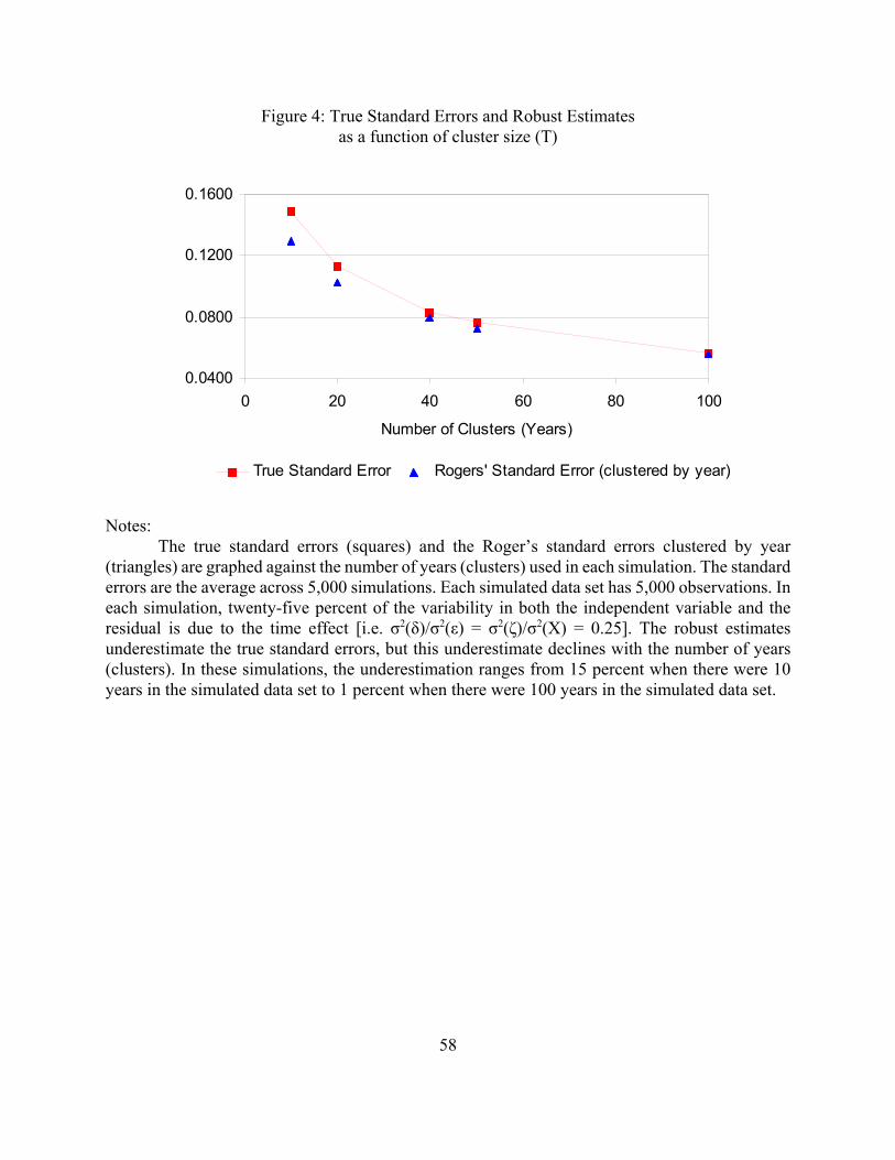
58

Figure 4: True Standard Errors and Robust Estimatesas a function of cluster size (T)

Notes:The true standard errors (squares) and the Roger’s standard errors clustered by year

(triangles) are graphed against the number of years (clusters) used in each simulation. The standarderrors are the average across 5,000 simulations. Each simulated data set has 5,000 observations. Ineach simulation, twenty-five percent of the variability in both the independent variable and theresidual is due to the time effect [i.e. σ2(δ)/σ2(ε) = σ2(ζ)/σ2(X) = 0.25]. The robust estimatesunderestimate the true standard errors, but this underestimate declines with the number of years(clusters). In these simulations, the underestimation ranges from 15 percent when there were 10years in the simulated data set to 1 percent when there were 100 years in the simulated data set.

0.0400

0.0800

0.1200

0.1600

0 20 40 60 80 100

Number of Clusters (Years)

True Standard Error Rogers' Standard Error (clustered by year)

59

Figure 5: Auto-correlation Patterns of Non-Fixed Firm Effects

Notes:This figure contains the auto-correlations of the residuals and the independent variable for

lags one through nine for the data structures used in Table 7. The specifications contain a fixed anda temporary firm component. φ is the fraction of the variance which is due to the fixed firm effectand φ is the first order auto-correlation of the non-fixed firm effect.

0.000.100.200.300.400.500.600.700.800.90

1 2 3 4 5 6 7 8 9

ρ=0.25,φ=0.00 ρ=0.00,φ=0.75ρ=0.25,φ=0.75 ρ=0.50,φ=0.50

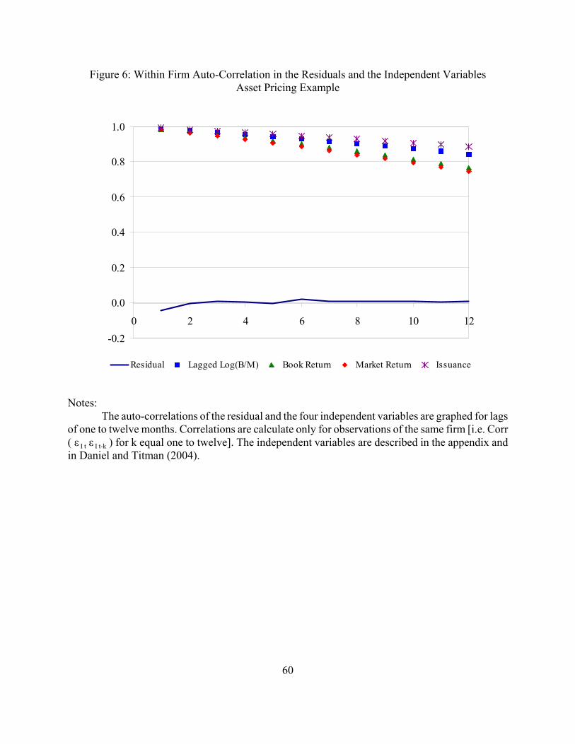
60

Figure 6: Within Firm Auto-Correlation in the Residuals and the Independent VariablesAsset Pricing Example

Notes:The auto-correlations of the residual and the four independent variables are graphed for lags

of one to twelve months. Correlations are calculate only for observations of the same firm [i.e. Corr( ε I t ε I t-k ) for k equal one to twelve]. The independent variables are described in the appendix andin Daniel and Titman (2004).

-0.2

0.0

0.2

0.4

0.6

0.8

1.0

0 2 4 6 8 10 12

Residual Lagged Log(B/M) Book Return Market Return Issuance

61

Figure 7: Within Month Auto-Correlation in the Residuals and the Independent VariablesAsset Pricing Example

Notes:The auto-correlations of the residuals and the four independent variables are graphed for lags

of one to twelve firms. Correlations are calculated only for observations of the same year [i.e. Corr( ε I t ε I-k t ) for k equal one to twelve]. The data was sorted by month, then by four digit industry, andthen by firm identifier (permco). The independent variables are described in the appendix and inDaniel and Titman (2004).

-0.2

0.0

0.2

0.4

0.6

0.8

1.0

0 2 4 6 8 10 12

Residual Lagged log(B/M) Book return Market return Issuance

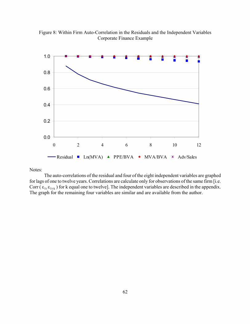
62

Figure 8: Within Firm Auto-Correlation in the Residuals and the Independent VariablesCorporate Finance Example

Notes:The auto-correlations of the residual and four of the eight independent variables are graphed

for lags of one to twelve years. Correlations are calculate only for observations of the same firm [i.e.Corr ( ε I t ε I t-k ) for k equal one to twelve]. The independent variables are described in the appendix.The graph for the remaining four variables are similar and are available from the author.

0.0

0.2

0.4

0.6

0.8

1.0

0 2 4 6 8 10 12

Residual Ln(MVA) PPE/BVA MVA/BVA Adv/Sales

63

Figure 9: Within Month Auto-Correlation in the Residuals and the Independent VariablesCorporate Finance Example

Notes:The auto-correlations of the residuals and four of the eight independent variables are graphed

for lags of one to twelve firms. Correlations are calculated only for observations of the same year[i.e. Corr ( ε I t ε I-k t ) for k equal one to twelve]. The data was sorted by month, then by four digitindustry, and then by firm identifier (gvkey). The independent variables are described in theappendix. The graph for the remaining four variables are similar and are available from the author.

0.0

0.2

0.4

0.6

0.8

1.0

0 2 4 6 8 10 12

Residual Ln(MVA) PPE/BVA MVA/BVA Adv/Sales