O K L A H O M A S T A T E U N I V E R S I T Y Boone Pickens School of Geology 105 Noble Research Center Stillwater, OK 74078-3031 405.744.6358, FAX 405.744.7841

Report for the Arbuckle-Simpson Hydrology Study:

Estimating Selected Hydraulic Parameters of the Arbuckle-Simpson Aquifer from the Analysis of Naturally-Induced Stresses

Estimating Selected Hydraulic Parameters of the Arbuckle-Simpson Aquifer

from the Analysis of Naturally-Induced Stresses

FINAL REPORT

by:

Khayyun Rahi Todd Halihan

Oklahoma State University

Boone Pickens School of Geology 105 Noble Research Center Stillwater, Oklahoma 74078

October 7, 2009 Stillwater, Oklahoma

Submitted to:

Oklahoma Water Resources Board 3800 North Classen Blvd. Oklahoma City, OK 73118

Cover: Photograph of Khayyun Rahi downloading a transducer at the Spears 2 Well

ii

Table of Contents

Table of Contents ........................................................................................................................ ii List of Figures ............................................................................................................................ iii List of Tables ............................................................................................................................. iv Acknowledgements ..................................................................................................................... v 1. Introduction ........................................................................................................................... 1 2. Previous Work ....................................................................................................................... 3 3. Specific Storage Theory ........................................................................................................ 6 4. Barometric Efficiency Theory ................................................................................................12 5. Transmissivity Theory ..........................................................................................................14 6. Arbuckle-Simpson Aquifer Monitoring ..................................................................................19

6.1. The Arbuckle-Simpson aquifer .......................................................................................19 6.2. Wells used for this study.................................................................................................21 6.3. Type of data collected and data processing and analyses. .............................................24

7. Analysis Methods .................................................................................................................25 7.1. Specific storage ..............................................................................................................25 7.2. Porosity from Improved Barometric Efficiency ................................................................27

8. Results and Discussion ........................................................................................................30 8.1. Specific storage ..............................................................................................................30 8.2. Porosity from the barometric efficiency ...........................................................................40

9. Conclusions ..........................................................................................................................45 10. References .........................................................................................................................46 11. Electronic Appendix ............................................................................................................48

Appendix E1. TRANSDUCER DATA COLLECTED IN STUDY .............................................48

iii

List of Figures

Figure 1. Idealized aquifer well system assumed for the earth tidal and barometric effects on

groundwater level. ...................................................................................................... 8

Figure 2. Idealized stratigraphic section for the Arbuckle-Simpson aquifer (after Puckette et al., 2009). ........................................................................................................................20

Figure 3. Water-level and atmospheric-pressure fluctuations for the well OWRB 91008. ..........22

Figure 4. Map of the Hunton Anticline portion of the Arbuckle-Simpson aquifer, showing wells equipped with pressure transducers ( 2 wells are present at the Spears Well site OWRB 101246 and 101247)......................................................................................23

Figure 5. Fluctuations in measured and compensated water level and barometric pressure for the OWRB 101246 well (Spears 1 test well). 26

Figure 6. One month of differenced water-level and barometric-fluctuation data for the well OWRB 101246 (Spears test well 1). ..........................................................................31

Figure 7. One month of measured water-level fluctuations (smoothed by differencing) compared to the modeled one in OWRB 101246 (Spears test well 1), 4/25-5/23/2008. ..............31

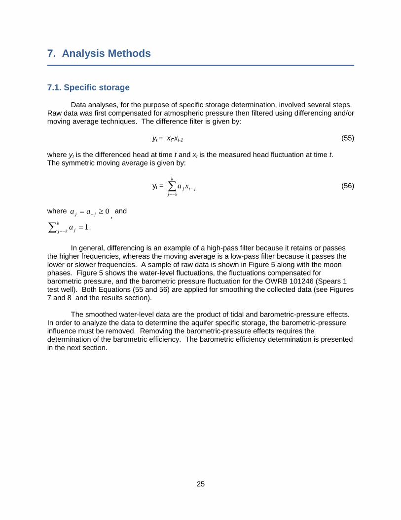
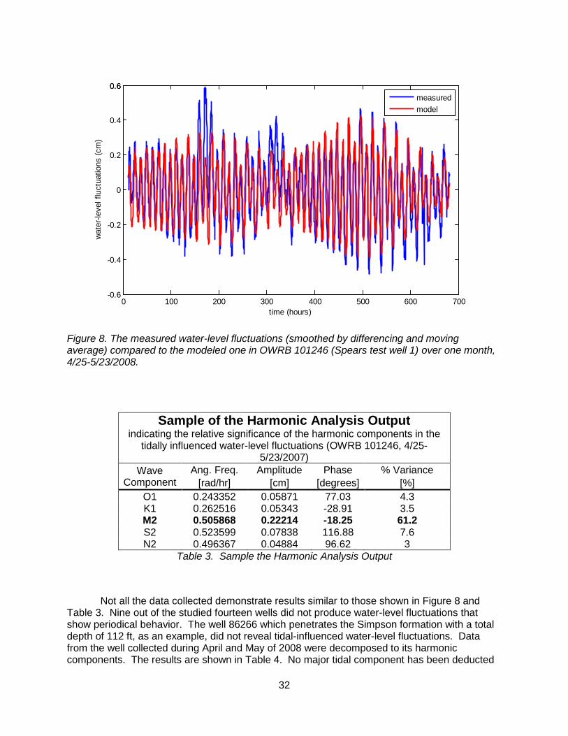
Figure 8. The measured water-level fluctuations (smoothed by differencing and moving average) compared to the modeled one in OWRB 101246 (Spears test well 1) over one month, 4/25-5/23/2008. .......................................................................................32

Figure 9. Model compared with measured water-level fluctuations for the well OWRB 86266. .33

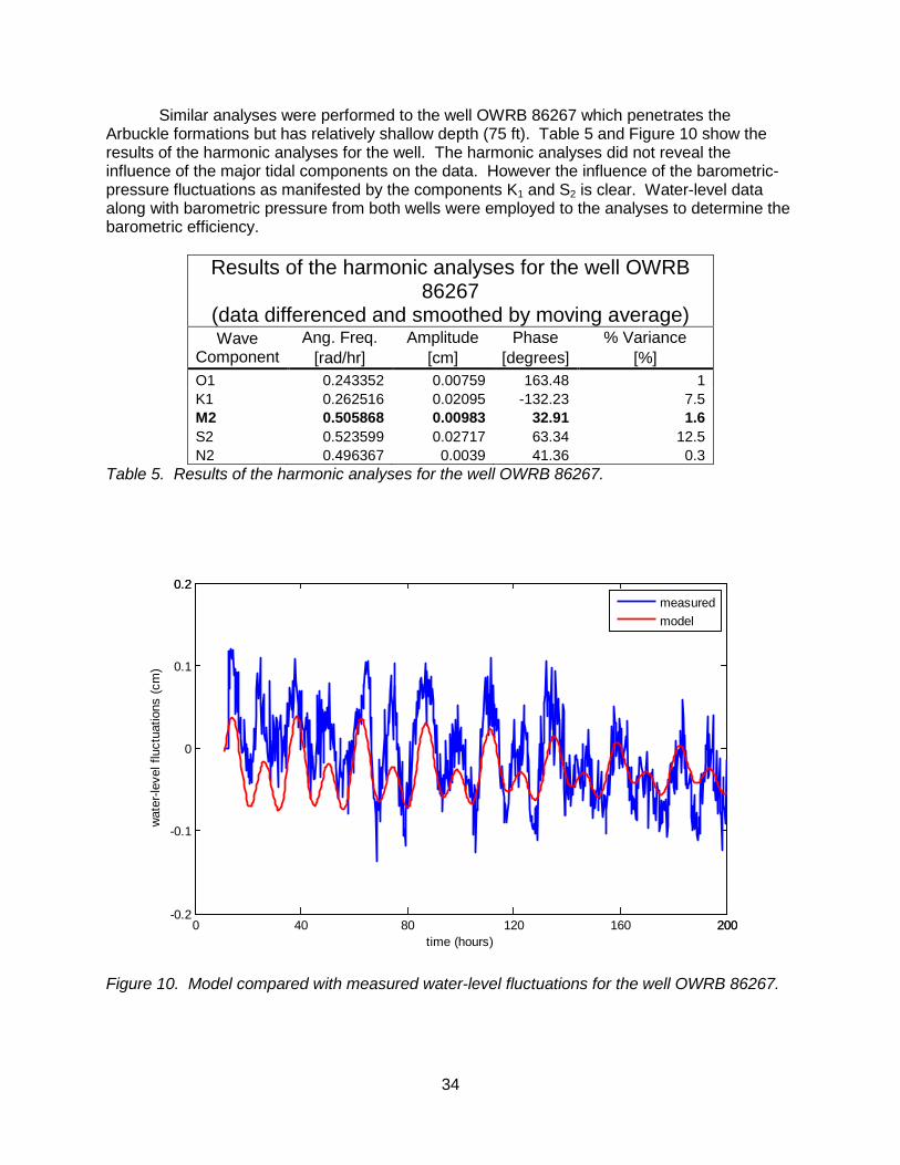
Figure 10. Model compared with measured water-level fluctuations for the well OWRB 86267. ..................................................................................................................................34

Figure 11. BE for well OWRB 101246 (Spears test well 1) as computed by Clark and the New model (Feb., 2007 –Jan., 2008). ................................................................................43

Figure 12. BE for OWRB 101247 (Spears test well 2) well as computed by Clark and the New model (Feb., 2007 –Jan., 2008). ................................................................................43

iv

List of Tables

Table 1. Harmonic components and some parameters of diurnal and semidiurnal equilibrium

tides. ..........................................................................................................................11

Table 2. Wells Used for Data Collection. ..................................................................................24

Table 3. Sample the Harmonic Analysis Output .......................................................................32

Table 4. Results of the harmonic analyses for the well OWRB 86266. .....................................33

Table 5. Results of the harmonic analyses for the well OWRB 86267. .....................................34

Table 6. Specific Storage Calculations .....................................................................................38

Table 7. Storativity and Porosity Calculations ..........................................................................39

Table 8. Porosity Calculations ..................................................................................................44

v

Acknowledgements

Thanks to Tim Sickbert, OSU Devon Laboratories and Chris Neel, Oklahoma Water

Resources Board for their assistance in the field. We would also like to thank the students from OSU who assisted us with this project including Jennifer Thorstad and Sassan Mouri. Paul Hsieh, USGS, provided critical input and assisted with tidal analysis software. Robert Ritzi, Wright State University and Scott Christenson, USGS, provided valuable assistance as well. Thanks also go out to Edward Mehnert, Illinois State Geological Survey (University of Illinois at Urbana-Champaign), Chris Neel (OWRB), and Noel Osborn (OWRB) for providing thoughtful and thorough reviews of this report.

1

1. Introduction

The Oklahoma Water Resources Board (OWRB) is conducting a hydrological study on

the Arbuckle-Simpson aquifer. One of the study objectives is to evaluate the water resources of the aquifer and put forward a management plan to utilize the resources in a manner that would preserve the ecological and environmental balance. An integrated part of the study is the use of a mathematical groundwater-flow and management model to assess and manage the groundwater resources. MODFLOW will be used by the USGS to construct a flow model of the aquifer.

Groundwater modeling techniques have increasingly proved their value in analyzing and evaluating groundwater systems. During the last four decades, groundwater hydrologists have relied heavily on modeling to further the understanding and, hence, in improving the assessment, development, and management groundwater resources. Almost all groundwater flow and transport models are designed to solve the relevant partial differential equation using numerical techniques such as finite-difference and finite-element. Usually the physical flow domain of an area to be modeled is replaced with a discretized model domain consisting of cells, blocks or elements depending on the numerical technique that is being employed. Knowledge of the aquifer parameters over the entire flow domain is essential to be able to calibrate a groundwater model. The mathematical modeling requires the assignment of a discrete value of the parameter to each cell or block in the model domain. These discrete values are designated as the model parameters. For a groundwater model to produce accurate output, the model parameters should accurately represent the hydraulic properties of the real aquifer system.

The aquifer parameters, which are essential to characterize the flow domain, are transmissivity, storage coefficient, and porosity. Traditionally, these parameters are determined by field or laboratory methods such us pumping and laboratory core tests. The laboratory results are of limited usefulness and hard to generalize since they represent disturbed core samples. The field methods are costly and of limited spatial extent (i.e. the results represent the specific site not the entire aquifer). Thus, alternative methods of parameters’ estimation that are less costly and could reflect the behavior of the entire aquifer (or large portions of it) are appealing. Several analytical and modeling approaches to estimate the aquifer hydraulic parameters are available. One approach is the use of the naturally induced stresses on the aquifer surfaces which cause water-level fluctuation within open wells.

Aquifers are subjected to mechanical stresses from natural processes such as mechanical forcing of the aquifer by ocean and earth tides or atmospheric-pressure loading. Earth and ocean tides are the product of lunar and solar-tidal forces. Changes in barometric pressure are induced by variation in temperature and circulation. Fluctuations of groundwater pressure due to these stresses are often reflected in the records of water-level monitoring wells.

The premise of this research is to analyze a confined aquifer-well system problem, in which pressure oscillation causes macroscopic water movement into and out of the well. The pressure oscillation is the product of the atmospheric-pressure fluctuation and dilation caused by the earth tides. Water-level fluctuations are analyzed and their amplitude and phase angle are resolved. The amplitude and the phase angle are functions, among other parameters, of the aquifer hydraulic properties. The resolved amplitude and phase angle are applied to the

2

computation of the transmissivity and storage coefficient (Bredehoeft, 1967; Hsieh and others, 1987; and Merritt, 2004).

The ratio of the change in water level in a well to the change in atmospheric pressure that produces it is known as the barometric efficiency (Be) (Jacob, 1940). The barometric efficiency may be considered as an index of the aquifer elasticity. In other words there should be direct relation between the barometric efficiency and the storage coefficient of a confined aquifer. A mathematical relationship linking Be to the porosity and the specific storage is employed to determine the Arbuckle-Simpson aquifer porosity. Generally, a high barometric efficiency indicates an ideal confined and elastic aquifer, while a low barometric efficiency indicates less than a perfect confined aquifer. Clark (1967) proposed a method to determine the barometric efficiency using the incremental changes in water level and the incremental changes in barometric pressure. However, it was mentioned through an earlier paper (Gregg, 1966) that “changes in water level due to changes in barometric pressure are difficult to distinguish and identify in the much larger change in water level due to tides”. Marine (1975) has indicated that calculating the Be is difficult for wells whose predominant water-level fluctuations are caused by earth tides.

Specific storage, porosity and barometric efficiency determination procedures and techniques for the Arbuckle-Simpson aquifer are the main concentration of this research. Transmissivity models are surveyed but not used to determine the aquifer transmissivity, due to their limited applicability. A portion of this research investigations and analyses are devoted to examining the Clark’s method and its consistency. Data from several wells of varying depths and locations were used for this purpose. The study revealed several difficulties in applying Clark’s method especially for short periods of observation. A new algorithm to calculate BE is introduced as part of this research. Reliable values for BE were obtained, and were used along with porosity figures inferred from well logs to get a more reliable values of the specific storage.

3

2. Previous Work

Water levels in wells are known to respond to earth tides and changes in atmospheric

pressure. Robinson (1939) published several hydrographs of wells in New Mexico and Iowa that reflect the influence of earth tides on water-level fluctuations. The author described the earth tide phenomena as reflecting the following characteristics:

1) Two daily cycles of fluctuations where the average daily retardation of cycles agrees closely with that of the moon transit;

2) The daily troughs of the water level coincide with the transit of the moon at the upper and lower culminations;

3) Periods of large regular fluctuations coincide with periods of new and full moon, whereas periods of small irregular fluctuations coincide with periods of first and third quarters.

Theis (1939) working with Robinson’s data and other data from Carlsbad, New Mexico, recognized that the water-level fluctuations could only be attributed to the dilation accompanying the tidal bulge. Jacob (1940) demonstrated how barometric and tidal effects can be used to determine the storage coefficient and porosity of an aquifer. He introduced the term “barometric efficiency” as an index of the elasticity of an aquifer system. The barometric efficiency is the ratio of the fluctuation in the water level in an open well to the change in atmospheric pressure at the surface. Jacob (1940), also, described the mechanics of the ocean tidal fluctuations and introduced the term “tidal efficiency “ which is the ratio of the change of water level in a well to a change in tide stage. The term “amplitude factor” replaced “tidal efficiency”, which is presented by Jacob (1950) and Ferris (1951) to describe the change of formation pressure caused by a spatially distributed change of pressure at land surface. Richardson (1956) reported water-level fluctuations resulted from earth tides effects in a well at Oak Ridge, Tennessee.

Melchior (1960) performed harmonic analyses of tidal fluctuations reported by other investigators. Melchior analyzed Robinson’s data from Iowa, Theis’ data from New Mexico, Richardson’s data from Tennessee, along with his data from the old Czechoslovakia, Belgium, and the Congo. Melchior indicated that the comparison of the amplitudes of the major waves showed “reasonable agreement” with amplitudes predicted from the equilibrium tidal theory. Melchior’s harmonic analyses concluded that the water-level fluctuations in these wells are linked to dilation produced by earth tides and revealed a great number of harmonic tidal components. Melchior (1964) stated that, “only five of these components are of real importance for groundwater fluctuation”. The five components comprise approximately 95 percent of the tidal potential and are: M2, a lunar wave with a period of 12h 25m 14s; S2, a solar wave with a period of 12h 00m, N2, a lunar wave with a period of 12h 39m 30s; K1, a luni-solar wave with a period of 23h 56m 4s; and O1, a lunar wave with a period of 25h 49m 10s (Table 1).

A relationship between the motion of water within an open well bore (taking into account the storage of water within the well bore) and pressure-head oscillations in the confined aquifer was developed by Cooper et al. (1965) to a seismic disturbance within the aquifer. The resulting equation established a relationship between the amplitude and phase lag of oscillations of the water level in the well to the amplitude of oscillations of pressure-head in the aquifer. The amplitude ratio between the water-level fluctuation within the well and the pressure head fluctuation within the aquifer is termed the amplitude response. Cooper et al. (1965) showed that the amplitude ratio is a function of the aquifer’s hydraulic properties (the transmissivity and storage coefficient), the radius of the well casing, the period of the forcing pressure, and the inertial effects of the water in the well.

4

Gregg (1966) developed a modification of Jacob’s tidal efficiency formula to compute the tidal efficiency adjusted for atmospheric-pressure change. Gregg’s study did not consider the earth tide effects on water-level fluctuations. He stated that “Water-level fluctuations caused by earth tides are 180 degrees out of phase with those caused by ocean tides.” Hence, any earth tide-caused fluctuations in the wells would be masked by the ocean tide-caused fluctuations. An important finding of Gregg’s study is that the tidal efficiency decreased with depth when measured in the same location. Since the tidal and barometric efficiencies add up to one (Jacob, 1940), this result suggests an increase with depth in the barometric efficiency. The barometric efficiency concept will be further examined and analyzed in later sections. Clark (1967) devised a method to estimate the barometric efficiency based on aperiodic, long-term pressure variation rising from the movement of air masses and the corresponding measured head changes in the well. Clark found that the atmospheric pressure had a period of about 12 hour, being high at 10 a. m. and p. m., and low at about 4 a. m. and p. m.

Bredehoeft (1967) followed the analyses of Cooper et al. (1965) and developed a theory for the response of the water level in the well to earth tides. The author showed that the inertial effects were negligible when the transmissivity of the aquifer was above (1 cm2/s). Bredehoeft (1967) considered the solid grains in bedrock are incompressible so that volume changes in the formations, due to the effect of the earth tides, are assumed equal to changes in the pore volume. Bredehoeft (1967) gave two possible approaches for analyzing observed water-level fluctuations deduced by earth tidal effects, namely, (1) to compare the fluctuation in the well with fluctuation that one would expect from tidal theory or (2) to compare the amplitude of the various tidal components obtained by harmonic analysis of the hydrograph with the theoretical amplitude of the particular waves. The author concluded that analyses of water-level fluctuations caused by the earth tide can be used to compute the specific storage and the porosity of the aquifer.

Marine (1975) compared crystalline rock aquifer parameters estimated from earth-tide analysis with the results of pumping tests. He found that the specific storage calculated from earth tides, using Bredehoeft (1967) model, was more than an order of magnitude higher than the specific storage determined from pumping tests. Marine (1975), also, calculated porosity using the same model and found that the computed porosity of “this slightly fractured crystalline aquifer...would (reach) 100%, an absurd value”. The author concluded that “the porosity is very sensitive to the barometric efficiency, which is extremely difficult to calculate for wells whose predominant water-level fluctuations are caused by earth tides.” Bredehoeft (1967) points out, ‘the porosity would represent an average value of a large volume in the vicinity of the well, a quantity which interests hydrologists and which is difficult, if not impossible, to determine by other means.’ Marine (1975) indicated that Bredehoeft (1967) statement is especially applicable for fractured rock where the overall porosity is difficult to estimate. Since the Arbuckle-Simpson aquifer is composed of fractured rock, it is certain that getting a measurement for porosity will be a difficult task. Marine (1975), also, concluded that porosity computed by Bredehoeft equation is very sensitive to both the specific storage and the barometric efficiency. In his calculation, a barometric efficiency of 50% resulted in 100% porosity for a sandy aquifer. In his final remarks, Marine (1975) agreed with Robinson’s (1971) conclusion that accurate calculation of aquifer parameters by analyzing tidal effect is difficult due to the lack of independent knowledge of several terms in the equations.

The response to earth tides of an open well screened in a confined aquifer was studied by Narasimhan and others (1984), who recognized the importance of well bore storage effects, the period of the tidal pulses, and the aquifer properties (permeability and specific storage). They applied a numerical model of saturated flow to demonstrate the qualitative importance of

5

these factors. Narasimhan et al. (1984) suggested that Bredehoeft (1967) analysis is internally inconsistent. They indicated that one cannot directly estimate the specific storage from earth tide response. Their point was that a confined aquifer responds to earth tide loading is in undrained fashion, while specific storage quantifies a drained behavior of the aquifer. Hsieh et al (1988) discussed the questions raised by Narasimhan et al. (1984) regarding the analysis of Bredehoeft (1967) and showed that it is possible to directly determine specific storage from undrained loading tests. They proceeded to conclude “thus it is not unreasonable that one can determine the specific storage from earth tide response”. The authors, also, showed that the Van der Kamp and Gale (1983) result reduced to the Bredehoeft result when the grains are assumed to be incompressible.

Hsieh et al (1987) adapted a graphical procedure to estimate transmissivity once the phase shift between the tidal dilatation of the aquifer and the water level response in the well was determined. They indicated that for phase analysis the concept of constant barometric efficiency is not sufficient for removal of barometric effects. Hsieh et al (1987) analyses showed that only the K1 and S2 tidal constituents are contaminated by barometric fluctuation. Hence the authors restricted their phase analysis to the M1 and O1 tidal component in order to isolate the effect of the barometric pressure fluctuations. The N2 constituent was disregarded, by their study, due to its small amplitude.

Ritzi et al, (1991) indicated that the earth tide influence occurs mainly at the four principal lunar and solar diurnal and semi-diurnal frequencies (O1, K1, M1, and S1). The authors analyzed the response of water level to earth tide, atmospheric pressure, and the combined effect of both stresses. Ritzi et al found estimates of storage coefficient are “nearly non-unique”. Transmissivity was uncorrelated to estimates of storage coefficient and can be determined by their analytical approach.

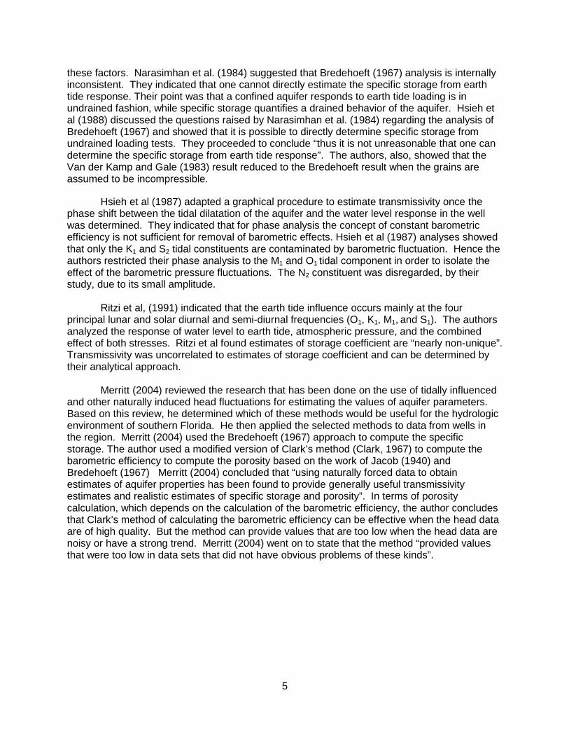
Merritt (2004) reviewed the research that has been done on the use of tidally influenced and other naturally induced head fluctuations for estimating the values of aquifer parameters. Based on this review, he determined which of these methods would be useful for the hydrologic environment of southern Florida. He then applied the selected methods to data from wells in the region. Merritt (2004) used the Bredehoeft (1967) approach to compute the specific storage. The author used a modified version of Clark’s method (Clark, 1967) to compute the barometric efficiency to compute the porosity based on the work of Jacob (1940) and Bredehoeft (1967) Merritt (2004) concluded that “using naturally forced data to obtain estimates of aquifer properties has been found to provide generally useful transmissivity estimates and realistic estimates of specific storage and porosity”. In terms of porosity calculation, which depends on the calculation of the barometric efficiency, the author concludes that Clark’s method of calculating the barometric efficiency can be effective when the head data are of high quality. But the method can provide values that are too low when the head data are noisy or have a strong trend. Merritt (2004) went on to state that the method “provided values that were too low in data sets that did not have obvious problems of these kinds”.

6

3. Specific Storage Theory

The applicable partial differential equation that describes the saturated groundwater

flow, in a homogeneous, isotropic, and confined aquifer, in radial coordinates, is (Jacob, 1950):

ts

TS

rs

rrs

∂∂

=∂∂

+∂∂ 1

2

2

(1)

where s is the drawdown at the well [L] in response to a discharge Q [L3/t], S is the storage coefficient of the aquifer [dimensionless], T is transmissivity [L2/t], r is the radial distance from the well [L], and t is time [t]

The storage coefficient of the aquifer, S, is given by:

)(ηαβγη += dS (2)

where γ is specific weight of water [N/m3], η is porosity [dimensionless], d is aquifer thickness [L], β is the compressibility of the water [m2/N], and α is the vertical compressibility of the formation [m2/N].

The storage coefficient is the specific storage [1/L] multiplied by the aquifer thickness. The water level in an open well tapping a confined aquifer responds to pressure head disturbances caused by natural or anthropogenic stresses. It fluctuates in response to earth-tide or barometric-pressure change stresses. The degree to which water-level fluctuates in response to these stresses is determined by the well dimensions, the transmissivity, storage coefficient, and porosity of the aquifer, Cooper et al. (1965) presented the following two equations to describe the harmonic pressure head disturbance in a confined aquifer (hf) and the water level response in the well (x) (Figure 1):

)sin( φω −= thh of (3)

)sin( txx o ω= (4) where

ho and xo are the amplitudes of pressure head and water-level fluctuations [L], respectively, t is time [t], ω = 2π/τ, it is angular frequency of the forcing function [1/t], τ period of fluctuation [t], and φ is the phase angle [radians].

The velocity of water-level fluctuation in the well casing is

7

=dtdx ωxo cos (ωt) (5)

The amplification factor (AF) as defined by Cooper et al. (1965) is given by:

o

o

o

o

pgx

hxAF ρ

== (6)

where ρ is density of the water in the well [M/L3], g is acceleration due to gravity [L/t2],

op is the pressure amplitude [F/L2]. Cooper et al. (1965) described the behavior of water level responding to a seismic event as that of a mechanical system subjected to forced vibration with viscous damping. They presented the following equation:

)sin()(2

1()(2

22

2

2

φωρ

αω

α −=−++ tHp

xKeiTr

Hg

dtdxKer

THgr

dtxd

e

ow

w

ew

e

w (7)

where

wr is radius of the well [L],

,83 dHH oe += it is the effective height of the water in the well [L],

oH is initial head in the aquifer [L], d is thickness of the aquifer [L],

21

)( TSrww

ωα = [Dimensionless]

eo Hp ρ is amplitude of the forcing function, Ker and Kei are Kelvin functions of order zero, and the other terms were defined earlier.

Several assumptions were considered in the development of Equation 7: 1) The well fully penetrates a homogeneous isotropic confined aquifer. 2) Inertial effects within the well were not neglected. 3) The forcing function on the aquifer is sinusoidal. 4) Drawdown is symmetric about the midpoint of the screen, which is (½) d. 5) Flow from the aquifer to the well across the well screen is uniform. 6) The water velocity within the well screen is vertical and uniform across a horizontal

section. 7) Friction forces due to flow within the well casing are negligible.

8

Figure 1. Idealized aquifer well system assumed for the earth tidal and barometric effects on groundwater level.

Equation 7 can be written in a reduced form as:

)sin(2 22

2

ηωρ

ωβω −=++ tHp

xdtdx

dtxd

e

oww (8)

where

))(2

1(2

2w

w

ew Kei

Tr

Hg α

ωω −= (9)

)(4

2

wew

w KerTHgr

αω

β = (10)

Equation 4 is analogous to the differential equation of motion of a mechanical system

subjected to forced vibration with viscous damping. When Equation 4 substituted into 7 the pressure amplitude ( op ) which will cause the water level to produce the oscillation described by equation 2 is given by:

21

222

22

0 )(2

)(2

1

+

−

−= w

e

ww

w

eeo Ker

THgr

KeiT

rHgHxp α

ωωα

ωρ (11)

9

Letting ω = 2π/τ and substituting Equation (11) into (6) yields the amplitude factor (AF) of Cooper et al. (1965) as:

21

222

2

22

)(4)(1

−

+

−−= w

wew

w KerTr

gHKei

TrAF α

τπ

τπα

τπ

(12)

Bredehoeft (1967) examined the amplitude factor equation (Equation 12) and stated “in

aquifers with transmissivities in excess of about 1 cm2/sec the change in pressure head due to the earth tide is equal to the change in water level in the well”; hence (AF) is assumed to be one. Neglecting the inertial effects, Bredehoeft (1967) presented the following equation for the change in head in a well produced by the tidal dilation t∆ :

s

t

Sdh

∆=− (13)

The tidal dilation ( t∆ ) is given by:

−

−−

=∆−−

agWlht

2621

21νν

, (14)

where t∆ is the tidal dilation [dimensionless],

υ is the Poisson ratio (≈0.25, Bredehoeft, (1967)) of the aquifer material [dimensionless], −

h and −

l are Love numbers at the surface of the earth [dimensionless], 2W is the tidal potential [L2/T2], and

a is the radius of the earth [L]. Substituting Equation 14 into 13 and rearranging the displacement of the water level in terms of the tidal potential ( 2W ), the specific storage ( sS ) of the aquifer is:

dhdW

aglh

vvSs

2621

21

−

−−

−=

−−

(15)

The tide potential is determined from the equation,

( ) ( ) ( )[ ]tbfgKtW m ,cos,,2 φβθφθ = (16) where

Km is the general lunar coefficient, taking into account the masses of the earth and moon,

the distance to the moon, and the earth’s radius, and it is equal to 53.7 cm (1.7618 ft), b is an amplitude factor [dimensionless] that has a distinct value for each tidal component with period τ ,

10

f (θ ) is the latitude function (dimensionless), and β (φ t) is a phase term that depends on the longitude φ and the Greenwich Mean Time (GMT) [t].

Merritt (2004) gave an approximation of Equation 15 as:

h

ws A

As

cmS 21

2

21210788.0

−

−

×= (17)

where 2wA is the amplitude of a harmonic component of W2 and period τ .

2wA is given by:

)(2 θbfgKA mw = (18)

Ah is the amplitude of a component of the head change of period τ ,and the other terms have been previously defined.

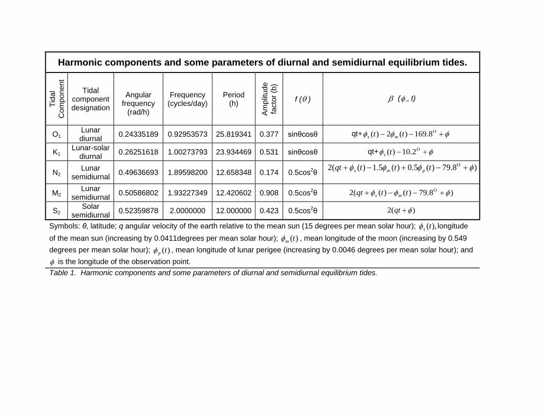
The gravitational acceleration, g, used for Equation 18 is 979 cm/sec2. The dimensionless terms of b, f (θ ), and β (φ t) were given by Merritt (2004), who correlated the work of Munck and McDonald (1960) and Doodson and Warburg (1941) and present it in a form useful for hydrologists. Merritt (2004) Tables 4 and 7 are combined and presented in Table 1 for five tidal components.

Harmonic components and some parameters of diurnal and semidiurnal equilibrium tides. Ti

dal

Com

pone

nt

Tidal component designation

Angular frequency

(rad/h)

Frequency (cycles/day)

Period (h)

Ampl

itude

fa

ctor

(b)

f (θ ) β (φ , t)

O1 Lunar diurnal 0.24335189 0.92953573 25.819341 0.377 sinθcosθ qt+ φφφ +−− Ο8.169)(2)( tt ms

K1 Lunar-solar

diurnal 0.26251618 1.00273793 23.934469 0.531 sinθcosθ qt+ φφ +− Ο2.10)(ts

N2 Lunar

semidiurnal 0.49636693 1.89598200 12.658348 0.174 0.5cos2θ )8.79)(5.0)(5.1)((2 φφφφ +−+−+ Οtttqt pms

M2 Lunar

semidiurnal 0.50586802 1.93227349 12.420602 0.908 0.5cos2θ )8.79)()((2 φφφ +−−+ Οttqt ms

S2 Solar

semidiurnal 0.52359878 2.0000000 12.000000 0.423 0.5cos2θ )(2 φ+qt

Symbols: θ, latitude; q angular velocity of the earth relative to the mean sun (15 degrees per mean solar hour); ),(tsφ longitude of the mean sun (increasing by 0.0411degrees per mean solar hour); )(tmφ , mean longitude of the moon (increasing by 0.549 degrees per mean solar hour); )(tpφ , mean longitude of lunar perigee (increasing by 0.0046 degrees per mean solar hour); and φ is the longitude of the observation point. Table 1. Harmonic components and some parameters of diurnal and semidiurnal equilibrium tides.

12

4. Barometric Efficiency Theory

The barometric efficiency eB (Jacob 1940) is given by

dbgdhBeρ

= (19)

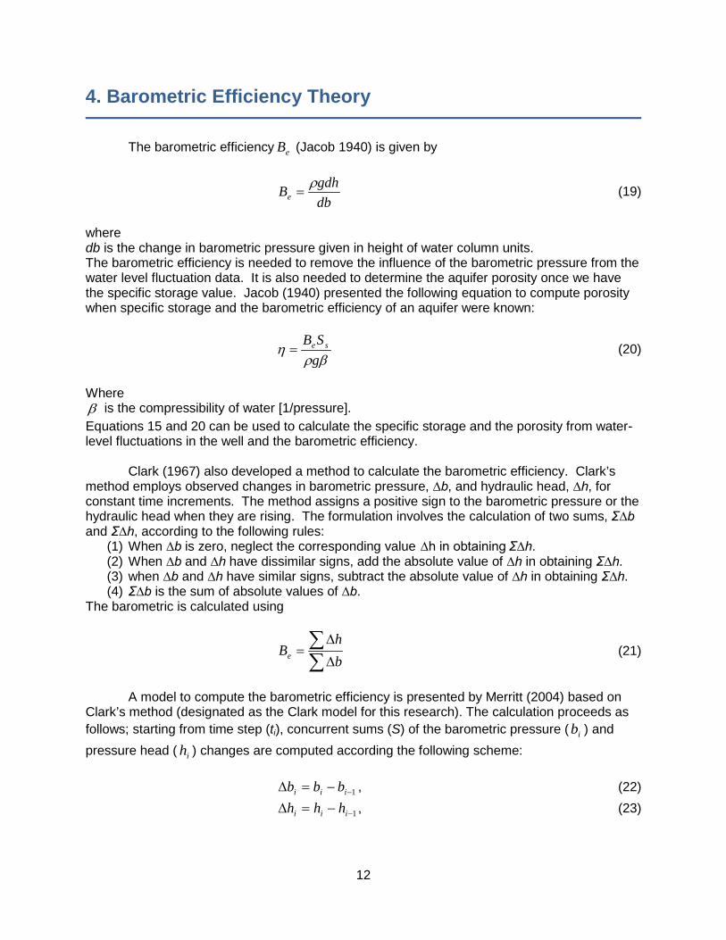
where db is the change in barometric pressure given in height of water column units. The barometric efficiency is needed to remove the influence of the barometric pressure from the water level fluctuation data. It is also needed to determine the aquifer porosity once we have the specific storage value. Jacob (1940) presented the following equation to compute porosity when specific storage and the barometric efficiency of an aquifer were known:

βρη

gSB se= (20)

Where β is the compressibility of water [1/pressure]. Equations 15 and 20 can be used to calculate the specific storage and the porosity from water-level fluctuations in the well and the barometric efficiency.

Clark (1967) also developed a method to calculate the barometric efficiency. Clark’s method employs observed changes in barometric pressure, ∆b, and hydraulic head, ∆h, for constant time increments. The method assigns a positive sign to the barometric pressure or the hydraulic head when they are rising. The formulation involves the calculation of two sums, Σ∆b and Σ∆h, according to the following rules:

(1) When ∆b is zero, neglect the corresponding value ∆h in obtaining Σ∆h. (2) When ∆b and ∆h have dissimilar signs, add the absolute value of ∆h in obtaining Σ∆h. (3) when ∆b and ∆h have similar signs, subtract the absolute value of ∆h in obtaining Σ∆h. (4) Σ∆b is the sum of absolute values of ∆b.

The barometric is calculated using

∑∑

∆

∆=

bh

Be (21)

A model to compute the barometric efficiency is presented by Merritt (2004) based on

Clark’s method (designated as the Clark model for this research). The calculation proceeds as follows; starting from time step (ti), concurrent sums (S) of the barometric pressure ( ib ) and pressure head ( ih ) changes are computed according the following scheme:

1−−=∆ iii bbb , (22)

1−−=∆ iii hhh , (23)

13

ii hbindex ∆∆= * , (24)

iib

ib bSS ∆+= −1 , (25)

iih

ih hSS ∆−= −1 if index >0 (26)

iih

ih hSS ∆+= −1 if index <0, and (27)

1−= i

hih SS if index=0 (28)

The calculation approach of this research is to employ Equations 17 and 20 for the determinations of the specific storage and the porosity. The barometric efficiency, for wells located in the Arbuckle-Simpson aquifer, was calculated by the Clark model and by a new model introduced as a part of this study (discussed in section 6).

14

5. Transmissivity Theory

The partial differential equation that describes the saturated groundwater flow in a

confined aquifer, in two dimensions is:

th

TS

yh

xh

∂∂

=∂∂

+∂∂

2

2

2

2

(29)

Where h is the hydraulic head [L], x and y are the Cartesian coordinates, and other terms as defined earlier. Groundwater levels in coastal aquifers that are in direct hydraulic contact with oceans or intersected by a regulated surface stream are subject to fluctuation due to tidal or change of stage effects. Ferris (1951), and Todd and Mays (2005) described the propagation of these effects within a confined aquifer by the following one-dimensional flow equation:

th

TS

xh

∂∂

=∂∂

2

2

(30)

where h is the net rise or fall in the piezometric surface relative to the mean sea or stream water level, and x is the distance inland from the surface water body. The boundary conditions are:

0/2sin tthh o π= ,at x=0 (31) and,

h=0 at x=∞ (32)

where oh is the amplitude of the fluctuation, and ot is the period of the ocean tide or river stage. The solution to Equation 26 with the applicable boundary conditions is

−= Ο− TtSx

tTehh o

TtSxo πππ

0

2sin (33)

Equation 33 defines a wave motion. The reduction of amplitude with distance is given by a factor of TtSxe 0π− . Jacob (1950) indicates that when the aquifer response is due to loading effects rather than head changes at the outcrop, the amplitude factor becomes, [ ] TtSx oe πηβαα −+ )( , where α is the aquifer skeleton compressibility.

From Equation 33, it follows that the range (twice the amplitude) xh of groundwater fluctuation at distance x from the shore line equals (Ferris 1951):

TtSxox

oehh π−= 2 (34)

15

Ferris (1951) studied the effect of surface stream stage fluctuation on groundwater level fluctuation. Groundwater fluctuations were measured in three observation wells in the City of Lincoln, Nebraska. Ferris defined the ratio ox hh 2 as the stage ratio; it is the ratio of groundwater fluctuation to the river stage fluctuation. Ferris (1951) adapted Equation 34 to compute the aquifer transmissivity in units of gallon per day per foot (7.48 gallons per cubic foot) as:

TtSxox

oehh 8.42 −= (35) The stage ratio is given by:

TtSx

o

x oeh

h 8.4

2−= (36)

or

TtSxhh oox 1.2/)2log( =− (37)

When the distance x plotted against the range ratio on a semi-log paper, the left hand side of Equation 37 represent the slope of this plot. If the change in the stage ratio is selected over one log cycle, the slope would be 1/∆x, where ∆x is the change of the distance corresponding to one log cycle change of the range ratio. Ferris (1951) presented the following equation to compute T (in gallon per day per foot) from the measurement of river and groundwater fluctuations:

2

4.4xtST

o∆= (38)

Hsieh and others (1987) developed an analytical method for estimating the aquifer

transmissivity from the phase shift associated with each tidal component. The method is similar to Cooper et al, (1965) but neglects the inertial effect of the water stored in the well bore. Hsieh and others (1987) approach is as follows. The amplitude response (A) is:

( ) 2122 −

+== FEhx

Ao

o , (39)

and

the phase shift φ is given by:

)/(tan 1 EF−−=φ , (40)

where,

)(2

12

wc Kei

Tr

E αω

−= , (41)

16

)(2

2

wc Ker

Tr

F αω

= , and (42)

ww rTS 2

1

=ωα , (43)

where

xo is the complex amplitude of the water-level oscillation in the well (L), ho is the fluctuating pressure head in the aquifer (L), rw is the radius of the screened or open portion of the well (L), rc is the radius of the well casing (L), ω =2π/τ is the frequency of the oscillations (T-1); τ is period of fluctuation (T), and Ker and Kei are real and imaginary Kelvin functions of order zero. The approach was developed for “single, laterally extensive aquifer that is homogeneous

and isotropic” (Hsieh et., al. 1987). Equations (39-43) shows the amplitude response A and the phase shift φ are both functions of two dimensionless parameters; Trc /2ω and wα . Hsieh and others (1987) used two other sets of dimensionless parameters that are “more convenient” for groundwater applications, 2/ crTτ and 22 / cw rSr . The authors plotted φ and A, respectively, versus 2/ crTτ for various values of 22 / cw rSr .

Measured water level fluctuations and measured or calculated earth tide potential are

regressed to determine the phase shift. The transmissivity is calculated by graphical methods. The method requires an independent estimate of the storage coefficient of the aquifer S. Merritt (2004) has concluded that the method of Hsieh et. el. (1987) is applicable to aquifers of transmissivities of less than 500 ft2 /d (5.4 cm2/sec).

Mehnert et al. (1999) applied the results of Cooper et al. (1967) as given by Equation 7

above to an externally forced aquifer (the external force is changes in atmospheric pressure). Mehnert et al. (1999) rewrote Equation 7 by expressing the amplitude of forcing function in terms of hydraulic head (xo) and using a trigonometric identity as:

)sin()cos()(2

1()(2 21

22

2

2

tctcxKeiTr

Hg

dtdxKer

THgr

dtxd

ww

ew

e

w ωωαω

α +=−++ (44)

17

where

1tan

tan21

+

−=

φ

φ

e

o

H

gxc , and (45)

and

1tan 22+

−=

φe

o

H

gxc (46)

Equation 44 has a two-part solution; homogeneous describing the transient-state and particular describing the steady-state. The steady-state solution as given by Mehnert (1998) and Mehnert et al. (1999) is presented hereafter The position of the water level in a well x(t) is given by:

)sin()cos()( 21 tdtdtx ωω += (47)

where

22224121

2

1 2 bbabcaccd+−+

+−−=

ωωωωω

, (48)

22224212

2

2 2 bbabcaccd+−+

+−−=

ωωωωω

(49)

e

ww

THKergr

a2

)(2 α= , and (50)

−=

TKeir

Hgb ww

e 2)(

12 αω

(51)

Equation 47 can be written as a single sine term using a the sine addition formula (Mehnert,

1999)

)sin()( φω −= tARtx (52)

18

where AR is the amplitude ratio and it is given by:

oo hdd

htx

AR22

21)( +

== (53)

and φ is the phase angle and it is given by:

−= −

2

11tandd

φ (54)

Mehnert et al., 1999 developed a “type curves” for by plotting AR versus dimensionless transmissivity (T''), where T’ = T/ωrw

2.

Mehnert et al., 1998 solved Equation 47 for a known values of T and S and generated plots of AR versus (T'') and φ versus (T''). The authors suggested using these plots as type curves to determine T. Once the AR is determined is determined, the value of (T'') is read from the “type curve” and T is determined from the dimensionless relationship T’=T/ωrw

2.

19

6. Arbuckle-Simpson Aquifer Monitoring

The Oklahoma Water Resources Board is conducting a hydrological study on the Arbuckle-Simpson aquifer. An integral part of the study is the use of a groundwater flow and management model (MODFLOW) to assess and manage the groundwater resources. The implementation of the flow model requires, as input, the model parameters. This research is intended to determine the Arbuckle-Simpson aquifer hydraulic parameters, using alternate methods, including; storage coefficient, porosity, and barometric efficiency. Data monitoring, collection, and processing program is laid out to cover the eastern parts of the aquifer, the Hunton Anticline. This section of the report includes a brief description of the Arbuckle-Simpson aquifer, a summary description of the wells employed for data monitoring and collection, type of data collected, and the approach for data presentation and analyses.

6.1. The Arbuckle-Simpson aquifer

The Arbuckle-Simpson aquifer is located within the Arbuckle Mountains physiographic province of South-Central Oklahoma. The aquifer outcrop underlies an area of about 500 square miles, but the total surface area of the aquifer may be larger and it is unknown. Fairchild et al (1990) provides a classic description of the area:

“The western part of the mountains, referred to as the Arbuckle Hills, is characterized by a series of northwest-trending ridges formed on resistant rocks that are intensively folded and faulted. The eastern part of the mountain, referred to as the Arbuckle Plains, is characterized by a gently rolling topography formed on relatively flat lying, intensively faulted limestone beds.”

The Arbuckle-Simpson aquifer is composed of several carbonate rock formations. The main formation is the Arbuckle and the Simpson groups of rocks. The Arbuckle group consists of limestone and dolomites that were deposited about 500 million years ago in Late Cambrian and Early Ordovician. The Simpson group overlay of the Arbuckle group. The Simpson group consists of sandstone, shale, and limestone that were deposited about 470 million years ago in Middle Ordovician time (Fairchild et al., 1990; Puckette et al., 2009). A typical stratigraphic section for the aquifer is shown in Figure 2.

20

System Group and Formation O

RD

IVIC

IAN

Viol

a

Gro

up Fernvale Formation

Viola Springs Formation

Sim

pson

Gro

up Bromide Formation

Tulip Creek Formation

McLish Formation

Oil Creek Formation

Joins Formation

Sim

pson

Aqu

ifer

Arbu

ckle

gro

up

West Spring Creek Formation

Kinblade Formation

Cool Creek Formation

McKenzie Hill Formation

Butterly Dolomite

Arb

uckl

e A

quife

r

CA

MB

RIA

N

Signal Mountain Formation

Royer Dolomite

Fort Sill Limestone

Tim

bere

d

Hill

Gro

up Honey Creek Limestone

Reagan Sandstone

Colbert Rhyolite

Figure 2. Idealized stratigraphic section for the Arbuckle-Simpson aquifer (after Puckette et al., 2009).

The aquifer is exposed at the land surface in three uplifted areas separated from each other by large high-angle faults. The western uplift is the Arbuckle Anticline. The Arbuckle Anticline resulted from intensive folding and faulting of a thick sequence of Paleozoic rocks which formed the ancestral Arbuckle Mountain. A unique view of the thick Paleozoic rock sequence and the complex structure of the Arbuckle Anticline is exposed in road cuts along Interstate 35. The eastern outcrop includes several structural features, of which the Hunton Anticline (the focus of this study) is the most prominent. The central outcrop is on the Tishomingo Anticline. The structural deformation on these two anticlines is much less pronounced than on the Arbuckle Anticline, and the topography is dominated by gently rolling plains (OWRB, 2003).

21

Groundwater flow is affected by the complex geologic features of the aquifer. Features such as folds, faults, fractures, and solution channels exert local influence on groundwater movements and flow rates. The flow rates can vary greatly locally and regionally. Groundwater moves slowly through fine fractures and pores and rapidly through solution-enlarged fractures and solution conduits. Generally, the aquifer is considered a carbonate rock aquifer exhibiting karst features especially in the western parts. Recharge to the aquifer is from precipitation that falls within the area. Fairchild and others (1990) estimated the long-term annual average precipitation in the area as 38.2 in. /year. Discharge from the aquifer is by evapotranspiration, through springs, and seeps, and by pumpage from wells (Fairchild et. al., 1990).

Surface water resources the aquifer area are represented by several perennial streams. Blue River, Pennington Creek, Mill Creek, Rock Creek, Delaware Creek, Oil Creek, and Sycamore Creek are the main streams draining the eastern parts of the aquifer area. These streams flow toward the south-southeast direction into the Washita River then to the Red River. The principle streams that drain the western part of the Arbuckle-Simpson aquifer area are Colbert, Hickory, Honey, Falls, Henryhouse, Cool, and Spring Creeks. Most of the streams are sustained throughout the year by groundwater discharge through springs or flow interception (Fairchild et al., 1990).

6.2. Wells used for this study

Fourteen wells distributed over the eastern part of the Arbuckle-Simpson aquifer are designated for this study. All the wells are equipped with some type of water level (pressure) fluctuations monitoring transducer. Of the 14 wells, there are two wells, Spears 1 and 2 were drilled as part of the Arbuckle-Simpson aquifer hydrological study program. The monitoring and data collection within these wells was done and administer by the Oklahoma State University (OSU), School of Geology. A barologger (a pressure transducer to monitor the atmospheric-pressure changed) was installed in the site of these two wells. One well, OWRB 89386 (USGS Fittstown), is belonged to and administered by the USGS. The rest of the wells are either private or belonged to the OWRB, but all the monitoring and data collection are executed and administered by the OWRB. Some of the data collected by the OWRB and the USGS were also analyzed for the purpose of this study.

The monitoring period varied from two months to more than one year. However the data

that were employed for the analysis ranges from one month worth of data to more than one year depending on the data quality and the significance of the well. Longer periods were used for deep wells that reflect the characteristics of confined aquifer. Barometric pressure was monitored at three well sites; OWRB 101246 (Spears test 1), OWRB 86267, and OWRB 86824. The atmospheric pressure monitoring periods were little more than one year for the well 101246, about 2 months for 86267, and for five months for the well 86824. Along with pressure readings, both water level and the barometric pressure transducers recorded the ambient temperature of the water or the air. Water levels and temperature of the Blue River were monitored for about a year in a location close to the Spears test wells. Water-level and barometric-pressure fluctuations were studied and analyzed to determine the specific storage and the porosity. The barometric efficiency was determined and used with the specific storage values to determine the porosity of the aquifer.

Not all the monitored wells were subjected to full analysis, several wells were not

considered because the collected data did reveal earth-tides influence. The measured water-

22

level data must demonstrate periodicity as an index of the tidal influence. The lack of periodicity behavior is shown in Figure 3. The spikes in water level measurement which oscillate between +7 to -7 cm every 24 yours present in Figure 3 may be resulted from an equipment malfunction. Lack of periodicity may be attributed to the low resolution of the measuring transducer, the aquifer type, and the saturated thickness at the well. The low resolution transducers were replaced in several wells, distributed over various parts of the aquifer, by high resolution ones. Data collected with the installed transducers did not reveal the earth-tidal influence, when decomposed by harmonic analysis, but showed strong atmospheric-pressure changes. This topic will be explored in more details in the next section.

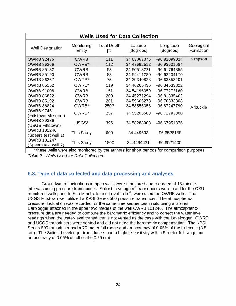
The locations of the study’s wells are shown in figure (4). Table (2) presents the wells

and some of their parameters. Two of the studied wells penetrate the Simpson Group (mainly sandstone) and the rest penetrate the Arbuckle Group (mainly carbonate rocks). The depths of most of the wells were taken from the records of the OWRB. The question mark on the depth of the well OWRB 86824 signifies doubts of the author about the reliability of this given depth. Data analysis (as will be seen later) indicates that the actual depth of this well may much more than the one that is reported.

Figure 3. Water-level and atmospheric-pressure fluctuations for the well OWRB 91008.

23

Figu

re 4

. Map

of t

he H

unto

n A

ntic

line

porti

on o

f the

Arb

uckl

e-S

imps

on a

quife

r, sh

owin

g w

ells

equ

ippe

d w

ith p

ress

ure

trans

duce

rs (

2 w

ells

are

pre

sent

at t

he S

pear

s W

ell s

ite O

WR

B 1

0124

6 an

d 10

1247

).

24

Wells Used for Data Collection

Well Designation Monitoring Entity

Total Depth [ft]

Latitude [degrees]

Longitude [degrees]

Geological Formation

OWRB 92475 OWRB 111 34.63067375 -96.82099024 Simpson OWRB 86266 OWRB* 112 34.47692512 -96.93631684 OWRB 85182 OWRB 53 34.50518221 -96.61764855

Arbuckle

OWRB 85190 OWRB 83 34.54411280 -96.62234170 OWRB 86267 OWRB* 75 34.39340823 -96.63553401 OWRB 85152 OWRB* 119 34.46265495 -96.84539322 OWRB 91008 OWRB 151 34.54196359 -96.77272160 OWRB 86822 OWRB 200 34.45271294 -96.81835462 OWRB 85192 OWRB 201 34.59666273 -96.70333808 OWRB 86824 OWRB* 250? 34.58555358 -96.87247790 OWRB 97451 (Fittstown Mesonet) OWRB* 257 34.55205563 -96.71793300

OWRB 89386 (USGS Fittstown) USGS* 396 34.58288903 -96.67951376

OWRB 101246 (Spears test well 1) This Study 600 34.449633 -96.6526158

OWRB 101247 (Spears test well 2) This Study 1800 34.4494431 -96.6521400

* these wells were also monitored by the authors for short periods for comparison purposes Table 2. Wells Used for Data Collection.

6.3. Type of data collected and data processing and analyses.

Groundwater fluctuations in open wells were monitored and recorded at 15-minute intervals using pressure transducers. Solinst Levelogger® transducers were used for the OSU monitored wells, and In Situ MiniTrolls and LevelTrolls®, were used the OWRB wells. The USGS Fittstown well utilized a KPSI Series 500 pressure transducer. The atmospheric-pressure fluctuation was recorded for the same time sequences in situ using a Solinst Barologger attached in the upper two meters of the well OWRB 101246. The atmospheric-pressure data are needed to compute the barometric efficiency and to correct the water level readings when the water-level transducer is not vented as the case with the Levelogger. OWRB and USGS transducers were vented and did not need the barometric compensation. The KPSI Series 500 transducer had a 70-meter full range and an accuracy of 0.05% of the full scale (3.5 cm). The Solinst Levelogger transducers had a higher sensitivity with a 5-meter full range and an accuracy of 0.05% of full scale (0.25 cm).

25

7. Analysis Methods

7.1. Specific storage

Data analyses, for the purpose of specific storage determination, involved several steps. Raw data was first compensated for atmospheric pressure then filtered using differencing and/or moving average techniques. The difference filter is given by:

yt = xt-xt-1 (55) where yt is the differenced head at time t and xt is the measured head fluctuation at time t. The symmetric moving average is given by:

yt = jt

k

kjj xa −

−=∑ (56)

where 0≥= − jj aa , and

∑ −==

k

kj ja 1.

In general, differencing is an example of a high-pass filter because it retains or passes

the higher frequencies, whereas the moving average is a low-pass filter because it passes the lower or slower frequencies. A sample of raw data is shown in Figure 5 along with the moon phases. Figure 5 shows the water-level fluctuations, the fluctuations compensated for barometric pressure, and the barometric pressure fluctuation for the OWRB 101246 (Spears 1 test well). Both Equations (55 and 56) are applied for smoothing the collected data (see Figures 7 and 8 and the results section).

The smoothed water-level data are the product of tidal and barometric-pressure effects.

In order to analyze the data to determine the aquifer specific storage, the barometric-pressure influence must be removed. Removing the barometric-pressure effects requires the determination of the barometric efficiency. The barometric efficiency determination is presented in the next section.

26

Figure 5. Fluctuations in measured and compensated water level and barometric pressure for the OWRB 101246 well (Spears 1 test well).

Next, the water-level data were resolved into its tidal components. The amplitude of

each tidal component is required for the analysis process (Equation 17). A linear regression model (least-square method) as presented by Hsieh et al. (1987) was employed for the harmonic analysis processes. The least-square method, which minimizes the sum of squares of a set of residuals (SSR), was used for the analyses. The SSR method of analysis is presented below.

Let xi be the ith measured pressure head fluctuation corresponding to time ti. The sum of

the squares of the residuals would be calculated as:

2

1 1

0 )sincos(2

1∑ ∑= =

+−−=

n

ijj

p

jjjjji tbta

ax

nSSR ωω (46)

where:

n is number of measured pressure head points, ti is the time of the ith pressure head measurement [t], ωi is frequency of the ith tidal component, the frequencies of the studied tides are precisely known and well documented, P=5 for this study, which represents the number of tidal components considered for the calculations, and

,0a ja , and jb are the 2P+1 unknown coefficients to be determined by the least-square method.

27

Equation 46 is differentiated with respect to the 2P+1 unknown coefficients to produce 2P+1 equations. Each equation is set to equal zero to minimize the sum of the squares. The resultant system of linear equations is solved to obtain the 2P+1 unknown coefficients. The amplitude of the jth tidal component ( jA ) is computed by:

2122 )( jjj baA += , and (47)

its phase angle ( jφ , (radians)) is given by:

)(tan 1jjj ab−=φ (48)

The calculations were restricted to the amplitude and phase angle of the five major tidal

components described earlier (Table 1). Two harmonic components, O1 and M2, and Equation 17 are used to calculate the storage coefficient. The rest were neglected because their influence judged by their amplitude was very small. For the two selected harmonic constituents, the amplitude and the phase shift was determined. The amplitude of the water-level fluctuations (Ah) and the amplitude of the earth-tide potential component ( 2wA ), were plugged into Equation 17 to compute the specific storage. Aw2 was computed using Equation 18 and the entries from Table 1. In many cases, O1 tidal component was neglected because its amplitude was so small compared to M2 (Table 3).

Data from all the monitored wells were analyzed. But, data of several wells did not

reveal the periodic behavior that is needed for the tidal analysis. The lack of periodicity was attributed to the transducer resolution and/or to the penetrated depth of a given well. An attempt was made to investigate the transducer issue. We installed the higher resolution Solinst transducer in the wells 85152, 86266, 86267, and 86824, and monitored the water-level fluctuations for about two months in each well. Well 86824 demonstrated finer scale periodic behavior with both tidal and barometric components. The new higher resolution datasets revealed that water-level fluctuations at the other wells are periodic; however, the signal is controlled by barometric-pressure changes, not tidal variations. In the next section, detailed data analysis is presented.

7.2. Porosity from Improved Barometric Efficiency

The barometric efficiency (Be) is commonly computed by the Clark’s method (Clark, 1967), which graphically relates the summation of the groundwater fluctuations to the summation of the atmospheric-pressure fluctuation that produces them. Be is needed in several applications. For this study, Be was used to determine the porosity of the aquifer as indicated by Equation 20.

Several authors indicated difficulty applying the Clark method to determine the Be. Hsieh et al (1987) considered removal of the barometric effects from the measured groundwater fluctuation using the Clark method as insufficient. The authors showed that only S2 and K1 harmonic components of the groundwater fluctuation bear the combined effects of earth tides and atmospheric-pressure loading. Hence they excluded these two components from the tidal analyses they preformed.

28

Marine (1975) attempted to determine the porosity of crystalline rock using storage coefficient and the barometric efficiency concept. The author concluded that the barometric efficiency is extremely difficult to calculate for wells whose predominant water-level fluctuations are caused by earth tides. In his calculation, Marine (1975) found a barometric efficiency of 50% resulted in a calculated porosity of 100 percent for a sandy aquifer. Marine (1975) ended up with porosities that were too high for the type of the aquifer he studied and even unrealistic. Marine (1975) reasoned the over estimation of the porosity to the barometric efficiency which he concluded is “very difficult” to determine.

The Clark model (Clark’s method), when applied to the data of this study, produced inconsistent results and in many instances resulted in efficiency values of more than 100 percent. Be of more than a 100 percent is physically unrealistic value. It appears that during periods of relatively high earth tides (new and full moon), the barometric effects on groundwater fluctuations are masked by the tidal effects. When this is the case, water-level fluctuations that are produced by tidal effects accounted by the Clark algorithm of calculation as if they were the product of atmospheric fluctuations. Therefore, the summation of the water-level changes increased unrealistically and resulted in Be of more than 100 percent.

An alternative algorithm is developed for the purpose of this study which minimizes the tidal interference with barometric effects. The new model subjects any data point to two tests ; the sign and the magnitude before deciding the fate of the given measurement, while the Clark model uses the sign test only. The new approach is outline hereafter.

The water-level fluctuation data were differenced and filtered to remove the influence of any linear trend. Starting from each time step (ti), concurrent sums of the barometric pressure ( bS ) and pressure head ( hS ) changes are computed according to the following algorithm:

1−−=∆ iii bbb , (49)

1−−=∆ iii hhh , (50)

ii hbindex ∆∆= * , (51)

iib

ib bSS ∆+= −1 , if index <0 and bh ∆≤∆ (52)

1−= i

bib SS , otherwise, (53)

iih

ih hSS ∆+= −1 if index <0 and bh ∆≤∆ (54)

1−= i

hih SS , otherwise. (55)

29

The barometric efficiency was determined using the Clark and the new model. Water-

level data used for the analysis are from the wells OWRB 85152, OWRB 86266, OWRB 86267, OWRB 86824 OWRB 97451, OWRB (USGS) 89386, and OWRB 101246 and 101247 (the Spears test wells). All of these wells penetrate the Arbuckle group formation with the exception of the well OWRB 86266 which taps the Simpson formation. Atmospheric pressure data used for the Be calculation were collected by the researchers using the Solinst Barologger. The barometric transducer was installed in at least three different wells for different time intervals. Data from (Merritt, 2004) related to the well HE-1087 were analyzed for the purpose of testing the new algorithm. This alternative method for calculating barometric efficiency was compared to the Clark method. Both methods were used to derive porosity calculations for the aquifer.

30

8. Results and Discussion

Fourteen wells (Table 2) of the Arbuckle-Simpson aquifer were monitored for their water-level fluctuations. Some of the wells did not show the presence of the tidal components that are characteristics of confined aquifer. Other wells water-level data was dominated by the influence of atmospheric pressure. Water-level fluctuations from wells tapping unconfined or semi-confined aquifer and/or influenced by barometric changes were not used for determination of specific storage and porosity. The results of the analyses are presented and discussed hereafter.

8.1. Specific storage

The specific storage was calculated from the groundwater-level fluctuations collected from the 14 wells listed in Table 2. The raw data was first filtered by differencing using Equation 55. A sample of differenced water-level and barometric-pressure fluctuations data are shown on Figure 6. Also shown in Figure 6 are the moon phases to demonstrate the tidal-magnitude effects on water-level fluctuations. The filtered data were analyzed using the linear regression model (Equations46-48), coded in FORTRAN, to determine the amplitude and the phase angle of the various tidal components (Hsieh et. al., 1987). Based on the finding of the linear regression, modeled water-level fluctuations were computed. The modeled fluctuations were compared to the measured water-level fluctuations. An example of the analyses and the comparison is shown in Figure 7. Visual examination of Figure 7 shows that the modeled data reflect a poor fit with the measured. Therefore data smoothing was carried a step further by applying the moving-average technique, (Equation 48). The fit of the model to the measured data was improved considerably as shown in Figure 8. The model parameters are shown in Table 3 for the data displayed in Figure 8. Table 3 also shows that M2 tidal component has the highest percent of variance. Percent of variance is a measure of the magnitude of influence of a given tide on tidally-influenced water-level fluctuations. The results listed in table three indicate that the M2 tidal component had the highest influence on the water-level fluctuations.

The regression process was restricted to five harmonic components; O1, K1, M2, S2, and

N2 (Table 1). The O1 and M2 tidal components were considered for the calculation of the specific storage. The N2 tidal component was disregarded due to its very small influence on the water-level fluctuations. The K1 and S2 constituents were neglected because they are influenced by the effects of the barometric and tidal loading (Hsieh et. al., 1987).

31

Figure 6. One month of differenced water-level and barometric-fluctuation data for the well OWRB 101246 (Spears test well 1).

0 100 200 300 400 500 600 700-2

-1.5

-1

-0.5

0

0.5

1

1.5

2

time (hours)

wat

er-le

vel f

luct

uatio

ns (c

m)

measuredmodel

Figure 7. One month of measured water-level fluctuations (smoothed by differencing) compared to the modeled one in OWRB 101246 (Spears test well 1), 4/25-5/23/2008.

32

0 100 200 300 400 500 600 700-0.6

-0.4

-0.2

0

0.2

0.4

0.60.6

time (hours)

wat

er-le

vel f

luct

uatio

ns (c

m)

measuredmodel

Figure 8. The measured water-level fluctuations (smoothed by differencing and moving average) compared to the modeled one in OWRB 101246 (Spears test well 1) over one month, 4/25-5/23/2008.

Sample of the Harmonic Analysis Output

indicating the relative significance of the harmonic components in the tidally influenced water-level fluctuations (OWRB 101246, 4/25-

5/23/2007) Wave

Component Ang. Freq. Amplitude Phase % Variance

[rad/hr] [cm] [degrees] [%] O1 0.243352 0.05871 77.03 4.3 K1 0.262516 0.05343 -28.91 3.5 M2 0.505868 0.22214 -18.25 61.2 S2 0.523599 0.07838 116.88 7.6 N2 0.496367 0.04884 96.62 3

Table 3. Sample the Harmonic Analysis Output

Not all the data collected demonstrate results similar to those shown in Figure 8 and

Table 3. Nine out of the studied fourteen wells did not produce water-level fluctuations that show periodical behavior. The well 86266 which penetrates the Simpson formation with a total depth of 112 ft, as an example, did not reveal tidal-influenced water-level fluctuations. Data from the well collected during April and May of 2008 were decomposed to its harmonic components. The results are shown in Table 4. No major tidal component has been deducted

33

in the data, even though the data were smoothed by two steps; differencing and moving average. The relative significant of a given tidal component on the water-level fluctuation is indicated by the value of percent variance in Table 4. The two important components considered for this study; O1 and M2, have very small influence (combined percent of variance of 0.7) on the water level movement. The highest influence on the data was attributed to the tidal components K1 and S2. These two components have the same frequency as the atmospheric-pressure fluctuations and were excluded from the analysis for the specific storage determinations. When the modeled data compared to the measured water-level fluctuation, the fit was poor (Figure 9).

Results of the harmonic analyses for the well OWRB 86266 (data differenced and smoothed by moving average)

Wave Component

Ang. Freq. Amplitude Phase % Variance [rad/hr] [cm] [degrees] [%]

O1 0.243352 0.00847 -166.92 0.7 K1 0.262516 0.03441 -141.31 11.2 M2 0.505868 0.00076 -139.74 0 S2 0.523599 0.05232 46.34 26 N2 0.496367 0.00134 -20.09 0

Table 4. Results of the harmonic analyses for the well OWRB 86266.

0 40 80 120 160 200200-0.2

-0.1

0

0.1

0.20.2

time (hours)

wat

er-le

vel f

luct

uatio

ns (c

m)

measuredmodel

Figure 9. Model compared with measured water-level fluctuations for the well OWRB 86266.

34

Similar analyses were performed to the well OWRB 86267 which penetrates the Arbuckle formations but has relatively shallow depth (75 ft). Table 5 and Figure 10 show the results of the harmonic analyses for the well. The harmonic analyses did not reveal the influence of the major tidal components on the data. However the influence of the barometric-pressure fluctuations as manifested by the components K1 and S2 is clear. Water-level data along with barometric pressure from both wells were employed to the analyses to determine the barometric efficiency.

Results of the harmonic analyses for the well OWRB 86267

(data differenced and smoothed by moving average) Wave

Component Ang. Freq. Amplitude Phase % Variance

[rad/hr] [cm] [degrees] [%] O1 0.243352 0.00759 163.48 1 K1 0.262516 0.02095 -132.23 7.5 M2 0.505868 0.00983 32.91 1.6 S2 0.523599 0.02717 63.34 12.5 N2 0.496367 0.0039 41.36 0.3

Table 5. Results of the harmonic analyses for the well OWRB 86267.

0 40 80 120 160 200200-0.2

-0.1

0

0.1

0.20.2

time (hours)

wat

er-le

vel f

luct

uatio

ns (c

m)

measuredmodel

Figure 10. Model compared with measured water-level fluctuations for the well OWRB 86267.

35

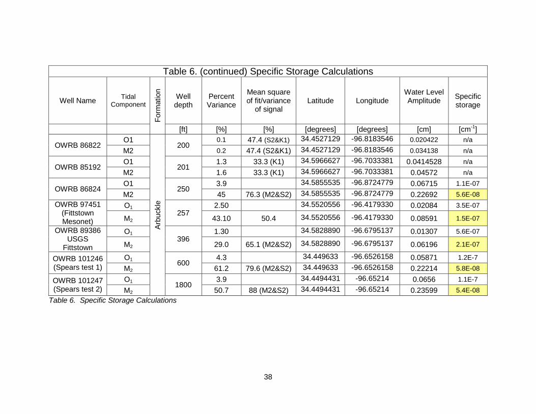
Results of all 14 wells studied are presented in Table 6. Two of these wells penetrate the Simpson Group (OWRB 86266 and 92475) and the rest are within the Arbuckle Group. The table includes the well number, depth, and location. The percent of variance and the mean square of fit/variance of signal are shown in the 5th and 6th columns of Table (6) respectively. Nine out of the 14 studied wells resulted in very low values of percent of variance and the mean square of fit/variance of signal which indicates that the data from these wells did not indicate the presence of O1 or M2 tides. These two tidal components were considered for the specific storage calculations. When they were not detected, water-level data can’t be utilized for the calculation process. Some wells (OWRB 86266, 86267, 85190, 91008, 86822, and 85192) show strong indication for K1 and S2 tides. These two tides are mainly solar component and caused partly by atmospheric-pressure oscillations. Therefore, they were not used for the specific storage determinations.

All nine wells which did not reflect the influence of the O1 and M2 tides on the water level fluctuations are relatively shallow. Their depths are 200 feet or less. These wells may tap a perched groundwater which behaves as shallow unconfined aquifer. Or, the wells may tap the major confined aquifer but for a small interval compared to total saturated thickness of the aquifer causing the tidal influence to be too small to detected (Bredehoeft, 1967). The Arbuckle-Simpson does not respond as confined over the entire area. It may demonstrate semi-confined to unconfined aquifer characteristics in several places (Fairchild et al., 1990). Regardless of the cause, it seems that the depth of the well and/or the degree of penetration is important factor in the generation of tidally-induced water-level fluctuations. Researchers concluded that earth tides influence water-level fluctuation in wells penetrating confined aquifers or deep, relatively stiff, and low-porosity unconfined aquifers (Bredehoeft, 1967; Weeks, 1979).

The specific storage values obtained from the five wells which demonstrate earth tides-induced water-level fluctuation ranges from 5.4E-8 to 5.6E-7 cm-1. The wells with the highest specific storage are located on the northeast part of the aquifer (OWRB 89386 (USGS Fittstown well) and OWRB 97452 (Fittstown Mesonet wells)). These two wells show stronger present of K1 and S2 tides compared to O1 and M2. This may indicate that these wells penetrating a semiconfined aquifer.

The values resulted by considering M2 tide only, range from 5.4E-8 to 2.1E-7 cm-1. The average value for the entire aquifer based on M2 results is about 1.056E-7 cm-1 (3.22E-6 ft-1). The average specific storage values (from M2 only) for the wells that are considered tapping confined portions of the aquifer is 5.6E-8 cm-1, and that for the wells tapping partly confined is 1.8E-7 cm-1. Values obtained for O1 tide are not reliable estimates because the percent variance for the tide was very small in all of the five wells. Therefore the considered value for the specific storage for the Arbuckle-Simpson aquifer as whole is 1.056E-7 cm-1 (3.22E-6 ft-1), for the confined portions is5.6E-8 cm-1 (1.7E-6 ft-1) and for the partly confined portions is 1.8E-7 cm-1(5.4E-6 ft-1).

The storage coefficient (storativity) of the aquifer was calculated for the wells of which specific storage was determined. Storage coefficient is the product of specific storage and aquifer thickness. Aquifer thickness obtained from the results of the 3-D earth-vision model applied to the Arbuckle-Simpson aquifer (Faith and Blome, 2008). Specific storage values used for the calculations were those resulted from the water-level fluctuations component M2. Table 7 shows the storativity values along with the aquifer thickness. The average storativity for the aquifer, as whole, is 0.011, for the confined portions is 6.3E-3, and for the semiconfined portions is 1.8E-2. Fairchild et al. (1990) reported average storativity of 0.008 based on pumping tests analysis. The estimated average storativity from this study is about 30% higher than that of

36

Fairchild et al. (1990). However, since Fairchild et al. (1990) values of the storage coefficient were determined by the modified Theis method, it is considered to be a storage coefficient of the confined portions of the aquifer. If this is the case, the storage coefficient determined resulted from this study (for confined portions) and that was determined by Fairchild et al. (1990) are very close to each other.

37

Table 6. Specific Storage Calculations

Well Name Tidal Component

Form

atio

n

Well depth

Percent Variance

Mean square of

fit/variance of signal

Latitude Longitude Water Level Amplitude

Specific Storage

[ft] [%] [%] [degrees] [degrees] [cm] [cm-1]

OWRB 92475 O1

Sim

pson

111 0.00 1.7 34.6306737 -96.8209902 0.0036576 n/a

M2 0.10 1.7 34.6306737 -96.8209902 0.006096 n/a

OWRB 86266 O1

112 0.7 37.9

(S2&K1) 34.4769251 -96.9363168 0.00847 n/a

M2 0.0 37.9 (S2&K1)

34.4769251 -96.9363168 0.00076 n/a

OWRB 85182 O1

Arbu

ckle

53 0.10 1.4 34.5051822 -96.6176485 0.010668 n/a

M2 0.00 1.4 34.5051822 -96.6176485 0.0003048 n/a

OWRB 86267 O1

75 1.0 22.9

(S2&K1) 34.3934082 -96.6355340 0.00759 n/a

M2 1.6 22.9 (S2&K1)

34.3934082 -96.6355340 0.00983 n/a

OWRB 85190 O1

83 0 47.1 (S2&K1)

34.5441128 -96.6223417 0.0088392 n/a

M2 83

0.1 47.1 (S2&K1)

34.5441128 -96.6223417 0.0131064 n/a

OWRB 85152 O1 119

0.2 2.5 34.4626549 -96.8453932 0.00522 n/a M2 0.00 2.5 34.4626549 -96.8453932 0.002 n/a

OWRB 91008 O1

151 0.2 33.9

(S2&K1) 34.5419636 -96.7727216 0.0143256 n/a

M2 0.9 33.9 (S2&K1)

34.5419636 -96.7727216 0.032004 n/a

38

Table 6. Specific Storage Calculations

Table 6. (continued) Specific Storage Calculations

Well Name Tidal Component

Form

atio

n

Well depth

Percent Variance

Mean square of fit/variance

of signal Latitude Longitude

Water Level Amplitude

Specific storage

[ft] [%] [%] [degrees] [degrees] [cm] [cm-1]

OWRB 86822 O1

Arbu

ckle

200

0.1 47.4 (S2&K1) 34.4527129 -96.8183546 0.020422 n/a M2 0.2 47.4 (S2&K1) 34.4527129 -96.8183546 0.034138 n/a

OWRB 85192 O1

201 1.3 33.3 (K1) 34.5966627 -96.7033381 0.0414528 n/a

M2 1.6 33.3 (K1) 34.5966627 -96.7033381 0.04572 n/a

OWRB 86824 O1

250 3.9 34.5855535 -96.8724779 0.06715 1.1E-07

M2 45 76.3 (M2&S2) 34.5855535 -96.8724779 0.22692 5.6E-08 OWRB 97451

(Fittstown Mesonet)

O1 257

2.50 34.5520556 -96.4179330 0.02084 3.5E-07

M2 43.10 50.4 34.5520556 -96.4179330 0.08591 1.5E-07

OWRB 89386 USGS

Fittstown

O1 396

1.30 34.5828890 -96.6795137 0.01307 5.6E-07

M2 29.0 65.1 (M2&S2) 34.5828890 -96.6795137 0.06196 2.1E-07

OWRB 101246 (Spears test 1)

O1 600 4.3 34.449633 -96.6526158 0.05871 1.2E-7

M2 61.2 79.6 (M2&S2) 34.449633 -96.6526158 0.22214 5.8E-08

OWRB 101247 (Spears test 2)

O1 1800 3.9 34.4494431 -96.65214 0.0656 1.1E-7

M2 50.7 88 (M2&S2) 34.4494431 -96.65214 0.23599 5.4E-08

39

Table 7. Storativity and Porosity Calculations

Well Name

Tida

l Com

p.

Well Depth Latitude Longitude Specific

Storage Aquifer

Thickness Storativity

Porosity from the

new method of

BE [ft]/[m] [degrees] [degrees] [cm-1] [m] [dim] [dim]

OWRB 86824 M

2 250/76.2 34.5855535

-

96.8724779 5.6E-08 1120 6.27E-03 0.14

OWRB 97451 257/78.1 34.5520556 -

96.4179330 1.5E-07 1010 1.5E-02 0.42

OWRB 89386

USGS Fittstown 396/120.7 34.5828890

-

96.6795137 2.1E-07 1028 2.15E-02 0.48

OWRB 101246

(Spears test 1)

600/183 34.449633 -

96.6526158 5.8E-08

1126 6.53E-03 0.15

OWRB 101247

(Spears test 2) 1800/549 34.4494431 -96.65214 5.4E-08 1127 6.08E-03 0.15

Table 7. Storativity and Porosity Calculations

40

8.2. Porosity from the barometric efficiency

The barometric efficiency (Be) is traditionally determined following the Clark model as described by Equations 22 through 28 (Clark, 1967; Merritt 2004). The Be was calculated for five wells; OWRB 86824, OWRB 89386 (USGS Fittstown), OWRB 97451 (Mesonet), OWRB 101246 (Spears test well 1), and OWRB 101247 (Spears test well 2). Water-level fluctuations and barometric pressure changes for a one-year period (Jan.27, 2007-Jan. 22, 2008) were employed for the calculation for the wells 101246 and 101247. As for the other three wells, the data used were for November and December, 2008 for the well 86824 and for April 15 to July 2, 2008 for the other two wells. The calculations were done for individual moon phases, complete moon cycles, and for several periods of more than one month each. The composite results are presented in Table 8 and Figures 10 and 11. The inconsistency in the Clark method can be seen in figures 10 and 11, which show Be values for individual moon phases calculated over the entire year. Results indicate higher Be values for First and Last Quarters and low BE values for Full and New moon phases. The Be values calculated with the Clark method range from 14 to 180 percent and tend to show high values for summer months for the wells 101246 and 101247, which are less than 50 meters apart. Results indicate that the Clark method is inconsistent and tends to overestimate Be. The variations for wells 89386 and 97451 are much less using the Clark method. However, all calculations indicate values of Be which are too high, in many instances physically unrealizable values of greater than 100 percent. Generally, the Be value is expected to range between 20 to 70 percent (Todd, 1980).

The First quarter moon, as used for this study, is the time interval from the time of the First quarter (where the Moon is at 90 degrees from the Sun-Earth axis) to the beginning of the Full moon. This means that the Moon is moving from its farthest position from the Sun-Earth axis to the position of the full moon where the Moon is lined along the axis. The gravity (tide) forces exerted by the combined effects of the Moon and the Sun are increased as the moon moves closer to full. The Full moon phase extends from the Full moon to the Last quarter. During the Full moon, as specified here, the combined tidal forces decrease gradually until its lowest point at the Last quarter. The Last quarter moon phase covers the time period from the last quarter, where the moon is again 90 degrees from the Sun Earth axis, to the New moon phase. Effects of tidal forces on the earth increase as the moon advance from the last quarter to the New moon. The New moon time starts at the New moon and ends at the First quarter moon position. The combined tidal forces decrease as the moon moves away from the New moon position. The highest tidal force exerted on the Earth is when the Moon and the Sun are aligned along the Earth-Sun axis during the New moon phase. Both the Sun and the Moon are pulling in the same direction during this phase. Generally, combined gravitational forces increase toward the Full and New moon phases and decrease toward the First and Last quarter moon phases. The highest BE values are associated with the last quarter and the second highest are associated with the first quarter. During New and Full moon, the tidal influence on groundwater fluctuations is at its maximum and most of the fluctuation probably is due to tidal forces, not to barometric pressure changes. The Clark method does not consider this issue; instead the method adds any water changes that are produced when the sign of the water-level change is opposite to that of the barometric pressure changes. If these changes are relatively high, their cumulative addition causes the sum of water-level changes to reach values higher than

41

the cumulative barometric pressure changes, hence producing a barometric efficiency of more than 100%. The BE values associated with the Full and New moons, though inconsistent, are more reasonable as will be demonstrated later. Several authors cited that the Clark model is inconsistent (Hsieh, et. al., 1987; Marine, 1975). Merritt (2004) concluded that the Clark method does not give acceptable results in several instances.

Close examination of Equation 26 is helpful to explain the effects of earth tides on the barometric efficiency calculations. Equation 26 states that when the water-level changes are attributed to barometric effects, these changes are added to the sum of water-level changes regardless of their magnitude. Whereas it is clear that when the magnitude of these changes is higher than the magnitude of the barometric pressure changes, they cannot be considered as entirely the product of barometric effects. These water-level fluctuations resulted from both barometric and earth-tide effects. As a result, it is more likely the computed barometric efficiency reaches values that are too high and may exceed 100 percent.

Based on this study outcome and the finding of previous research (Hsieh, et. al., 1987, Marine, 1975; Merritt, 2004), the Clark method to determine the barometric efficiency can be considered questionable and its use may produce uncertain results. The method applicability is limited to the cases when the moon is in Full to Last quarter and from the New moon to the First quarter. When applied, the method should be considered with caution because the barometric efficiency may be overestimated as indicated by Marine (1975).

A new model for Be determination that overcomes deficiencies in the Clark method is presented here. The model filters the water level as well as the barometric pressure data to remove the effects of the earth tides from the water-level fluctuations. Hence, only the barometric pressure induced water-level fluctuations and the barometric fluctuations that produce them are employed for the calculation of the barometric efficiency. The new model is represented by Equations 34 through 40. Results of the new model are presented in Figures 10 and 11 to compare them with the Clark method. The new model produced consistent barometric efficiency values for all time intervals and all five wells. Be values range from 46 to 56 percent for the Arbuckle-Simpson aquifer, compared to Be of 68 to more than 90 percent as computed by the Clark method. When comparing the results of the two models, Clark’s method as applied to water-level fluctuations produced during the Full and New moons produces results close to the new model. However, these values are still higher for the Clark method as compared to the new model. Porosity as calculated by Equation 20 is very sensitive to Be values. Overestimating Be may result in erroneously high porosity for the aquifer.

The porosity was determined for each well of the five wells and shown in Table 8. The porosity was computed using Equation 20. Values used for the computations are: density of water as 1 gm/cm3, acceleration due to gravity (g) as 979 cm/sec2, and the compressibility of water as 2.1*10E-10 cm-sec2/gm (Marine, 1975). The resulting porosities, when barometric efficiency values resulted from Clark’s method were utilized, were unreasonably high. The average porosity for the Clark method was 40% while that of the new model was 26%. Porosities from the wells OWRB 89386 and 97451 are very high compared to the other three wells. These two wells are considered penetrating partially confined portions of the aquifer. The specific storage values that were calculated for these wells should not be considered reliable, because the Bredehoeft theory (Bredehoeft, 1967) was derived for ideal confined aquifer. Accordingly, the

42

porosity values should not be weighted equally along those of the other three wells which provide an average porosity of 0.15. Therefore, the porosities of the wells OWRB 101246 and 101247 (the Spears test wells) and OWRB 86824, computed using barometric efficiencies of the new model are considered representative of the Arbuckle-Simpson aquifer.

The conclusion that may be drawn from the results of porosity calculation is that barometric efficiency values used for the calculation should be tested for consistency and accuracy. The new model to determine the barometric efficiency is consistent and doesn’t overestimate its value. The porosity calculated by this approach is the primary porosity and it is for confined aquifer only. Therefore, water-level fluctuation data from confined aquifer only should be utilized for the porosity determination. As for the barometric efficiency, the new model is recommended.

43

Figure 11. BE Barometric efficiency for the well OWRB 101246 as computed by the Clark and the new model. Points for the full moon are enlarged to make the full moon quarter easier to observe. The gray area indicates barometric efficiencies that are physically unrealizable.

Figure 12. BE for OWRB 101247 (Spears test 2) well as computed by the Clark and the new model. Points for the full moon are enlarged to make the full moon quarter easier to observe. The gray area indicates barometric efficiencies that are physically unrealizable.

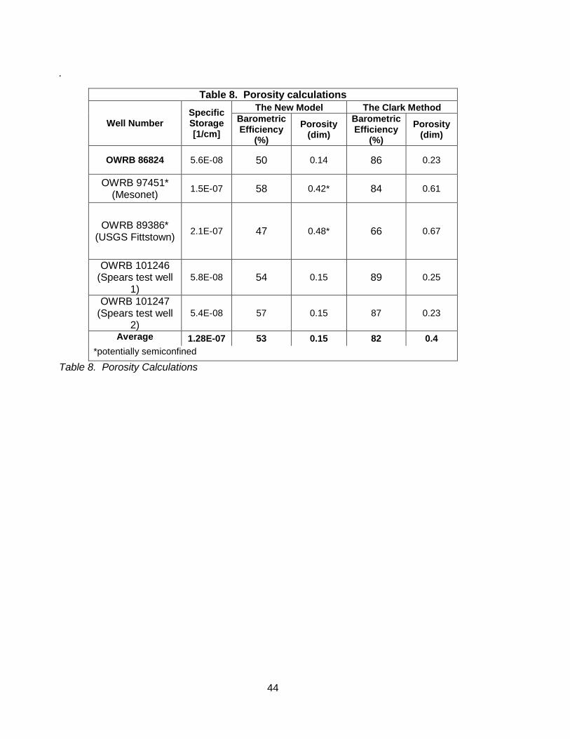
44

.

Table 8. Porosity calculations

Well Number Specific Storage [1/cm]

The New Model The Clark Method Barometric Efficiency

(%) Porosity

(dim) Barometric Efficiency

(%) Porosity

(dim)

OWRB 86824 5.6E-08 50 0.14 86 0.23

OWRB 97451* (Mesonet) 1.5E-07 58 0.42* 84 0.61

OWRB 89386* (USGS Fittstown) 2.1E-07 47 0.48* 66 0.67

OWRB 101246 (Spears test well

1) 5.8E-08 54 0.15 89 0.25

OWRB 101247 (Spears test well

2) 5.4E-08 57 0.15 87 0.23

Average 1.28E-07 53 0.15 82 0.4 *potentially semiconfined

Table 8. Porosity Calculations

45

9. Conclusions

Earth-tides and barometric-pressure fluctuations affect the water-level within an aquifer. The tidally and barometric pressure-induced water-level fluctuations within a well are a function of the aquifer hydraulic parameters, well parameters, natural stress frequencies and amplitudes. The well water-level fluctuations were analyzed to determine the specific storage, storage coefficient, and the porosity of the Arbuckle-Simpson aquifer. Barometric efficiency is determined because it is needed to determine the porosity. Data from 14 wells of variable depths and variable time intervals were employed for the analyses. The average specific storage for the aquifer is 1.056E-7 cm-1 (3.22E-6 ft-1). The resulting storage coefficient is 0.011 and an average porosity of 0.15.

The barometric efficiency was computed by the Clark model and by a new model introduced as part of this study. Results indicate that the Clark method is inconsistent and tends to overestimate Be as the method may produce efficiencies of more than 100 percent (physically unrealistic values) when applied to data collected during the First or Last quarter moon phases. Based on the outcome of this study, and the findings of previous research (Hsieh, et. al., 1987, Marine, 1975; Merritt, 2004), the Clark method is questionable when used to determine the barometric efficiency and may produce inconsistent results. The method applicability is limited to the cases when the moon is in Full to Last quarter and from the New moon to the First quarter. Even during these periods, the Clark method may over estimate Be. The new model showed consistency and produced reasonably acceptable values for the barometric efficiency when applied to five wells for different time periods. The average barometric efficiency value for these wells, as determined by the new model, is approximately 53 percent. This barometric efficiency may be considered an indication value for a large region of the aquifer since barometric effects are regional in nature. While this method improved the barometric efficiency estimate, the resulting porosity values were higher than expected and may only represent the fracture porosity for the aquifer.

46

10. References

Bredehoeft, J.D., 1967, Response of well-aquifer systems to earth tides, Journal of

Geophysical Research v. 72, no. 12, pp. 3,075-3,087.

Clark, W.E., 1967, Computing the barometric efficiency of a well, Journal of the Hydraulics Division, American Society of Civil Engineers, v. 93, no. HY4, pp. 93-98.

Cooper, H.H., Jr., Bredehoeft, J.D., Papadopoulos, I.S., and Bennett, R.R., 1965, The response of well-aquifer systems to seismic waves: Journal of Geophysical Research, v. 70, no. 16, p. 3,915-3,926.

Doodson, A. T., and Warburg, H. D., 1941 (reprinted 1966), Admiralty manual of tides: London, Her Majesty’s Stationary Office.

Fairchild, R. W., Hanson, R. L., and Davis, R. E., 1990, Hydrology of the Arbuckle Mountain area, South-Central Oklahoma, Oklahoma Geological Survey, Circular 91, pp112.

Faith, J., and Blome, C.D., 2008, Three-dimensional EarthVision modeling for ground-water resource applications: Arbuckle-Simpson aquifer, southern Oklahoma, Abstract, AGU Fall Meeting 2008, Abstract H41G-0968.

Ferris, J.G., 1951, Cyclic fluctuations of water level as a basis for determining aquifer transmissibility, International Geodesy Geophysics Union, Assoc. Sci. Hydrology Gen. Assembly, Brussels, v. 2, pp. 148-155; duplicated 1952 as U. S. Geological Survey Groundwater Note 1.

Gregg, D.O., 1966, An analysis of ground-water fluctuations caused by ocean tides in Glynn County, Georgia: Groundwater, v. 4, no. 3, pp. 24-32.

Hsieh, P.A., Bredehoeft, J.D., and Farr, J.M., 1987, Determination of aquifer transmissivity from earth tide analysis, Water Resources Research, v. 23, no. 10, pp. 1824-1832.

Hsieh, P.A., Bredehoeft, J.D., and Rojstaczer, S. A., 1988, Response of well-aquifer systems to earth tides: Problem revisited, Water Resources Research, v. 24, no. 3, pp. 468-472.

Jacob, C.E., 1940, On the flow of water in an elastic artesian aquifer, American Geophysical Union Transactions, part 2, pp. 574-586; duplicated 1953 as U. S. Geological Survey Groundwater Note 8.

———1950, Flow of groundwater in Engineering Hydraulics, edited by H. Rouse, John Wiley and Sons, New York.

Marine, I.W., 1975, Water-level fluctuations due to earth tides in a well pumping from slightly fractured rock, Water Resources Research, v. 11, no. 1, pp. 165-173.

Melchior, P., 1960, Die gezeiten in unteriridschen flussigkerten, Erdoel Kohle, no. 13, 312-317, cited by Bredehoeft, J.D., 1967, Response of well-aquifer systems to earth tides, Journal of Geophysical Research v. 72, no. 12, pp. 3,075-3,087.

Melchior, P., 1964, Earth tides in Research in Geophysics, v. 2, edited by H. Odishaw, Cambridge, Massachusetts, Massachusetts Institute of Technology Press, pp. 183-193.

47

Merritt, M. L., 2004, Estimating hydraulic properties of the Floridan aquifer system by analysis of earth-tide, ocean-tide, and barometric effects, Collier and Hendry Counties, Florida, U.S. Geological Survey, Water-Resources Investigation Report 03-4264, 70p.

Munk, W.H., and McDonald, G.J.F., 1960, The rotation of the earth, London, Cambridge University Press.

Narasimhan, T.N., Kanehiro, B.Y., and Witherspoon, P.A., 1984, Interpretation of earth tide responses of three deep, confined aquifers: Journal of Geophysical Research, v. 89, no. B3, p. 1,913-1,924.

OWRB (Oklahoma Water Resources Board), 2007, The Arbuckle-Simpson aquifer hydrological study, available at: http://www.owrb.ok.gov.

Puckette, J., Halihan, T., Faith, J., 2009, Characterization of the Arbuckle-Simpson aquifer, Report to the Oklahoma Water Resources Board, 56 pp plus appendices.

Richardson, R. M., 1956, Tidal fluctuations of water level observed in wells in east Tennessee, Trans. Am. Geophys. Union, no. 37, pp 461-462.

Ritzi, R.W., Jr., Sorooshian, S., and Hsieh, P.A., 1991, The estimation of fluid flow properties from the response of water levels in wells to the combined atmospheric and earth tide forces: Water Resources Research, v. 27, no. 5, pp. 883-893.

Robinson, E.S., and Bell, R.T., 1971, Tides in confined well-aquifer systems: Journal of Geophysical Research, v. 76, no. 8, pp. 1,857-1,869.

Robinson, T. W., 1939, Earth-tides shown by fluctuations of water levels in wells in New Mexico and Iowa, Trans. Am. Geophys. Union, v. 20, pp 656-666.

Theis, C. V., 1939, Earth tides as shown by fluctuations of water level in artesian wells in New Mexico, Intern. Union Geodesy and Geophysics, Washington, D. C. (U.S. Geological Survey open-file report, 10 p.

Todd, D. K., 1980, Groundwater Hydrology, 2nd ed., John Wiley and Sons, New York, 535p

Todd, D. K., and Mays, L. W., 2005, Groundwater Hydrology, 3rd ed., John Wiley and Sons, Inc., New York, 636 p.

Weeks, E. P., 1979, barometric fluctuations in wells tapping deep unconfined aquifers, water Resources Research, v. 15, no.5, pp. 1,167-1,176.

Van der Kamp, G., and Gale, J.E., 1983, Theory of earth tide and barometric effects in porous formations with compressible grains, Water Resources Research, v. 19, no. 2, pp. 538-544.

48

11. Electronic Appendix

Appendix E1. TRANSDUCER DATA COLLECTED IN STUDY