Estimating Recharge Uncertainty using Bayesian Model ...€¦ · Estimating Recharge Uncertainty using Bayesian Model Averaging and Expert Elicitation with Social Implications A Thesis

Estimating Recharge Uncertainty using Bayesian Model Averaging and Expert Elicitation with Social Implications

A Thesis

Presented as Partial Fulfillment of the Requirements for the

Degree of Master of Science

with a

Major in Water Resources

in the

College of Graduate Studies

University of Idaho

by Matthew Reeves

May 2009

Major professor: Dr. Fritz Fiedler

ii

AUTHORIZATION TO SUBMIT

THESIS This thesis of Matthew A. Reeves, submitted for the degree of Master of Science with a

major in Water Resources and titled " Estimating Recharge Uncertainty using Bayesian

Model Averaging and Expert Elicitation with Social Implications" has been reviewed in

final form. Permission, as indicated by the signatures and dates given below, is now granted

to submit final copies to the College of Graduate Studies for approval.

Major Professor ________________________________Date______________ Fritz Fiedler

Committee Members ________________________________Date______________

Paul Allan ________________________________Date______________

Gary Johnson Department Administrator ________________________________Date______________

Jan Boll Discipline's College Dean ________________________________Date______________

Donald Blacketter

Final Approval and Acceptance by the College of Graduate Studies ________________________________Date______________

Margrit von Braun

iii

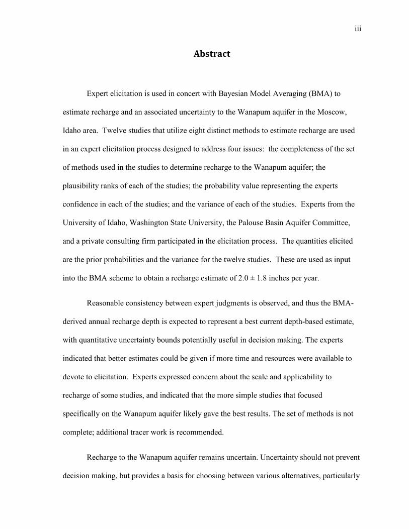
Abstract

Expert elicitation is used in concert with Bayesian Model Averaging (BMA) to

estimate recharge and an associated uncertainty to the Wanapum aquifer in the Moscow,

Idaho area. Twelve studies that utilize eight distinct methods to estimate recharge are used

in an expert elicitation process designed to address four issues: the completeness of the set

of methods used in the studies to determine recharge to the Wanapum aquifer; the

plausibility ranks of each of the studies; the probability value representing the experts

confidence in each of the studies; and the variance of each of the studies. Experts from the

University of Idaho, Washington State University, the Palouse Basin Aquifer Committee,

and a private consulting firm participated in the elicitation process. The quantities elicited

are the prior probabilities and the variance for the twelve studies. These are used as input

into the BMA scheme to obtain a recharge estimate of 2.0 ± 1.8 inches per year.

Reasonable consistency between expert judgments is observed, and thus the BMA-

derived annual recharge depth is expected to represent a best current depth-based estimate,

with quantitative uncertainty bounds potentially useful in decision making. The experts

indicated that better estimates could be given if more time and resources were available to

devote to elicitation. Experts expressed concern about the scale and applicability to

recharge of some studies, and indicated that the more simple studies that focused

specifically on the Wanapum aquifer likely gave the best results. The set of methods is not

complete; additional tracer work is recommended.

Recharge to the Wanapum aquifer remains uncertain. Uncertainty should not prevent

decision making, but provides a basis for choosing between various alternatives, particularly

iv

when quantitative values can be clearly communicated. To place the BMA recharge

estimate in a decision making context, the broad effects of physical and social uncertainty on

the decision making process are assessed in collaboration with a social scientist. Decision

makers have an incentive to adopt the Precautionary Principle without physical and social

certainty guiding decisions. The BMA estimate can quantitatively inform decision makers

in developing management plans consistent with this principle, and can be updated as new

recharge estimates are made. The overarching management strategy best equipped to deal

with uncertainty appears to be some form of adaptive management which involves scientists,

managers, decision-makers, and the public.

v

Acknowledgements

I would like to thank my advisor Dr. Fritz Fiedler for his support and critical input to

this thesis and my committee members Dr. Gary Johnson and Dr. Paul Allan for their

support and help in reviewing this thesis. I would like to thank Dr. Fritz, Fiedler, Dr Gary

Johnson, Dr. Dale Ralston, Dr. Jim Osiensky, Dr. Kent Keller, Dr. Mike Barber, Dr. Paul

McDaniel, Mr. Steve Robischon, Dr. Tim Link, and Dr. Jan Boll for their participation in the

elicitation process. I would like to thank Katie Bilodeau for her help in co-authoring the

interdisciplinary chapter. I would like to thank Waters of the West and the NSF/GK-12

program for their funding support. Lastly, I would like to thank my wife and family for their

support and encouragement.

vi

Table of Contents

Abstract .................................................................................................... iii

Acknowledgements ................................................................................... v

Table of Contents ..................................................................................... vi

List of Figures .......................................................................................... ix

List of Tables ............................................................................................. x

Chapter I .................................................................................................... 1

Palouse Basin Overview ...................................................................................................... 1

1.0 Introduction ................................................................................................................ 1

1.1 Geologic Setting ......................................................................................................... 2

1.2 Objectives and Scope ................................................................................................. 3

Chapter II ................................................................................................... 5

Literature Review ................................................................................................................. 5

2.0 Recharge Estimation Methods ................................................................................... 5

2.1 Palouse Basin Recharge Investigations ...................................................................... 7

2.2 Bayesian Model Averaging ...................................................................................... 11

2.3 Expert Elicitation of Prior Probabilities ................................................................... 13

2.4 Uncertainty and Decision Making ........................................................................... 14

Chapter III ............................................................................................... 16

Methods .............................................................................................................................. 16

3.0 Recharge Estimation Using Historical Data ............................................................ 16

vii

3.2 Expert Elicitation ..................................................................................................... 22


Chapter IV ............................................................................................... 30

Results ................................................................................................................................ 30

4.0 Recharge Estimation Using Historical Data ............................................................ 30

4.1 Expert Elicitation ..................................................................................................... 33


Chapter V ................................................................................................ 45

Social and Scientific Uncertainty and Implications on Decision Making ......................... 45

5.0 Scientific and Social Uncertainty ............................................................................. 45

5.1 Decision Making Approaches .................................................................................. 46

5.2 Physical and Social Scientific Factors Affecting Decision Making Approaches .... 49

5.3 Uncertainty and Decision Making ........................................................................... 51

5.4 Palouse Basin ........................................................................................................... 52

5.4 Summary .................................................................................................................. 56

Chapter VI ............................................................................................... 58

Conclusions and Recommendations .................................................................................. 58

6.0 Conclusions .............................................................................................................. 58

6.1 Recommendations for Additional Research ............................................................ 59

References ............................................................................................... 61

viii

Appendix A ............................................................................................. 66

Elicitation Data .................................................................................................................. 66

Appendix B ............................................................................................. 70

Summaries of Studies that Estimate Recharge in the Palouse Basin ................................. 70

ix

List of Figures

Figure 1: Location of Palouse Basin ....................................................................................... 1

Figure 2: Map showing the location of the USGS, Bond, Brandt, Moscow #2, and Moscow

#3 wells .................................................................................................................................. 18

Figure 3: Cone of depression scenarios ................................................................................ 21

Figure 4: Prior probability distribution of recharge studies .................................................. 34

Figure 5: Aggregated prior probabilities of recharge studies ............................................... 36

Figure 6: Aggregated variance of recharge studies ............................................................... 37

Figure 7: Weighted prior probabilities of individual studies ................................................ 40

Figure 8: Variance within and between studies .................................................................... 41

Figure 9: Probability distribution of recharge (not to scale) ................................................. 43

x

List of Tables

Table 1: Water level for USGS observation well (39N 05W 07DDC1) and pumping

volumes for Moscow #2 and #3 ............................................................................................. 19

Table 2: Studies Included in the Expert Elicitation .............................................................. 26

Table 3: Five year moving averages of water level, pumping, and recharge ....................... 30

Table 4: Average recharge for the Wanapum aquifer system .............................................. 31

Table 5: Results of Bayesian Model Averaging ................................................................... 42

1

Chapter I

Palouse Basin Overview

1.0 Introduction

The Palouse Basin is home to the cities of Moscow, Idaho and Pullman, Washington

and covers approximately 235 square miles (Douglas, 2007) in eastern Washington and

northwestern Idaho. Several smaller towns such as Colfax, Albion, and Palouse in

Washington, and Potlatch and Viola in Idaho as well as rural residents make up the rest of

the population of the basin(approximately 52,000; Community Water Information System).

The University of Idaho is located in Moscow, Idaho, and eight miles to the west is

Washington State University in Pullman, Washington. The location of the Palouse Basin is

shown in figure 1.

(wikimedia.org, 1 Sept. 2008) (Douglas et al, 2007)

Figure 1: Location of Palouse Basin

http://commons.wikimedia.org/wiki/

2

Moscow, ID and Pullman, WA have been the major groundwater users in the

Palouse Basin since the first wells were drilled in the late 1800s. According to I. C. Russell

(1897) the first artesian well was the M. C. True well drilled in Pullman, WA in 1894. It

supplied 30,000 gallons per day and had sufficient pressure to cause water to rise in a pipe

20 feet above the ground surface. Eleven wells that were completed in the flood plain of the

South Fork of the Palouse River by 1896 were flowing artesian wells. In the Moscow, ID

area, 14 wells had been drilled since 1890 and 10 of those were flowing artesian wells in

1891, but by 1896 water levels had dropped to 8 to 9 feet below land surface. Russell had

the foresight to see that the supply of water was not unlimited and made this observation.

“Several of the wells at Pullman are allowed to flow, thus wasting a large volume of water and decreasing the pressure. If the blessings accompanying the discovery of an excellent water supply are to be maintained, all wells should be closed when not in use” (Russell, 1897).

Water use in Pullman and Moscow increased as more development in the basin

occurred. The groundwater used by both cities is drawn from a sole source aquifer system

with an upper and a lower aquifer known as the Wanapum aquifer and Grande Ronde

aquifer, respectively. Water level declines have become an increasing problem since the

development of the resource in the late 1800’s.

1.1 Geologic Setting

This is a brief summary of the basin geology intended to provide a general

understanding only; for in-depth geological descriptions, see Foxworthy and Washburn

(1963), Barker (1979) and Bush (2005). The Palouse Basin is underlain by Miocene Era

basalt and sediments which lie on pre-Tertiary crystalline basement rock. The basin is

capped by Pleistocene loess which ranges from a few feet to several hundred feet thick (Lum

3

et al, 1990). The Miocene basalt belongs to the Columbia River Basalt Group (CRBG). The

Wanapum and Grande Ronde aquifers are contained in the Wanapum and Grande Ronde

basalts and sediments of the Latah Formation can be found interbedded, underlying, and

overlying the basalts (Bush, 2005).

The upper Wanapum aquifer system consists of basalts from the Priest Rapids

Member of the Wanapum Formation, sedimentary interbeds of the Latah Formation and the

underlying sediments of the Vantage Formation. The Wanapum aquifer is tapped by the

City of Moscow and rural homeowners with private wells. The lower Grande Ronde aquifer

is housed in the Grande Ronde Formation and is separated from the Wanapum aquifer by the

thick sedimentary interbed of the Vantage Member of the Miocene Ellensburg Formation.

The cities of Moscow and Pullman as well as the University of Idaho and Washington State

University rely heavily on the Grande Ronde aquifer to supply their water needs. Across the

Pacific Northwest, the CRBG contains important aquifers, many of which are in a state of

decline, thus estimating recharge and uncertainties are broadly important to sustainable

management of regional aquifers.

1.2 Objectives and Scope

Multiple studies have been conducted that estimate recharge in the Palouse Basin.

The estimates vary widely and most have no bounds of uncertainty associated with them.

This study focuses on determining the uncertainty in recharge to the Wanapum aquifer.

Also, the interaction of social and scientific uncertainty and their coupled effect on decision

4

making is discussed in an interdisciplinary chapter. The specific objectives of this study are

to:

1. Analyze historical water level and pumping data to calculate a recharge rate for

the Wanapum aquifer and an associated estimate of uncertainty,

2. Use Bayesian Model Averaging and expert elicitation to combine previous

estimates of recharge and determine an aggregate recharge rate and

corresponding level of uncertainty for the Wanapum aquifer, and

3. Assess the interaction between scientific uncertainty and social uncertainty, and

their coupled effect on the decision making process.

5

Chapter II

Literature Review

2.0 Recharge Estimation Methods

Recharge estimation can generally be classified into physical, tracer, or numerical

modeling approaches. Scanlon (et al., 2002) compiled a comprehensive review of these

methods. This section is a summary of Scanlon (et al., 2002) for the purpose of providing

the necessary background to understand this work, and the reader is referred to Scanlon (et

al., 2002) for additional detail.

The water budget, or mass balance equation is the basis for many of the different

methods and a simplified equation applicable to basins is shown in Equation 2-1.

� � �� (2-1)

P is the precipitation; Qs is the surface water discharge out of the basin; ET is

evapotranspiration; and R is the recharge. P, Qs, and ET are measured or estimated and the

residual is equal to the recharge, assuming that these are the only fluxes into and out of the

basin and no change in storage. The accuracy of this method is dependent on the accuracy

with which the different parameters are determined. Basin or watershed water budgets

typically rely on one or more streamflow gauging stations, point measurements or spatial

distributions of precipitation, and uniform or distributed calculations of ET from

temperature and land use data.

Channel water budgets have been used to estimate surface water loss between

gauging stations. Recharge calculated via channel water budget can be overestimated

6

because of bank storage, evapotranspiration, and perched aquifers or shallow water tables

not connected to the main aquifer. The ground water table fluctuation method is based on a

water budget of an aquifer, using the assumption that rises in ground water levels in

unconfined aquifers are due to recharge. Pumping, entrapped air, and changes in

atmospheric pressure may introduce error in the calculations and these components can be

accounted for.

Seepage meters have been successfully used to measure seepage flux in lakes,

streams, swamps, and tidewater areas at locations throughout the U.S. They provide only

point estimates of flux and many measurements are necessary to determine a representative

value of infiltration. Lysimeters are another physical technique that can be used to measure

recharge. They are however expensive to construct and maintain and are better suited for

evaluation of evapotranspiration at specific locations.

Multiple tracer techniques exist for determination of recharge including: heat tracers,

isotopic tracers, applied tracers, historical tracers and environmental tracers. Diurnal or

annual temperature fluctuations’ can be used with inverse modeling software to estimate

hydraulic conductivity. Recharge rates can be estimated from hydraulic head measurements

coupled with the hydraulic conductivity. Isotopic tracers such as oxygen and hydrogen can

provide information on recharge sources, but quantification of actual recharge rates is very

difficult. Bromide, 3H, and organic dyes are chemical tracers that when applied at the soil

surface or in the soil profile can be used to estimate recharge rates. Sampling is done via

test holes or trenching months or years after application, and the vertical distribution of the

tracers is used to determine the velocity and recharge. Historical tracers are a result of

human activity such as nuclear testing or contaminant spills and have been used to estimate

7

recharge rates over the past 50 years, and provide qualitative evidence of recharge.

However, due to the uncertainties in concentration, source location and behavior of

contaminants, quantifying rates of recharge is problematic and difficult. Chloride is an

environmental tracer that is produced naturally in the earth’s atmosphere and can be used to

estimate recharge rates. Chloride concentration is inversely related to drainage in the

unsaturated zone pore water, and this relationship results in more accurate estimation of

recharge at low drainage rates. Chloride mass balance has been widely used and is useful to

estimate recharge rates up to 300 mm/year.

Darcy’s law can be used to estimate recharge, and while this method is easy to apply,

it requires information on large scale effective hydraulic conductivity and hydraulic

gradient. Estimates are often highly uncertain due to variability in hydraulic conductivity.

This is especially true with unsaturated hydraulic conductivity where values vary over

orders of magnitude based on moisture content.

Numerical modeling has proven a useful tool for estimation of groundwater

recharge. Ground water flow models are developed based on hydrologic data and calibrated

to reproduce historical trends. Uncertainties in hydraulic conductivities directly affect

recharge estimation and may result in non unique solutions as long as the ratio of recharge to

hydraulic head is constant.

2.1 Palouse Basin Recharge Investigations

Palouse water resource investigations were initiated in 1897 by I. C. Russell. He

conducted a water supply reconnaissance of southeastern Washington which included the

8

Palouse and its artesian wells (Russell, 1897). Many investigations and reports have been

completed since then regarding the geology, hydrogeology, aquifer properties, and recharge

to the Grande Ronde and Wanapum aquifers. The geology and hydrogeology are discussed

in depth by Foxworthy and Washburn (1963), Jones and Ross (1972), Barker (1979), and

Bush (2005). Stevens (1960) and Foxworthy and Washburn (1963) used a rudimentary

water budget analysis to estimate the recharge to the basalt aquifers through the loess.

Single values for precipitation and evapotranspiration for the entire Basin were used in the

water budget. Stevens indicated an error estimate of 25 % in his report. Fealko (2003) used

a mass balance of the Paradise Creek watershed to probabilistically calculate the recharge to

the Wanapum aquifer. Gauging stations were used to determine surface water run-off, and

Parameter-elevation Regressions on Independent Slopes Model (PRISM) data were used to

distribute precipitation spatially. PRISM data for temperature values was used in potential

evapotranspiration calculations with Hargreaves method. Dungel (2007) built on Fealko’s

work and used Stella software to develop a systems model of the Palouse Basin. The

hydrologic component of the model was based on a mass balance of the Palouse Basin. The

Basin was divided into six different sub-basins and PRISM data were used to determine

precipitation and evapotranspiration. Distributed actual ET was computed using the

procedure of Thornthwaite and Mather. The model used data from several surface water

gauging stations and output an estimate of recharge for the Wanapum and Grande Ronde

aquifers.

Ground water flow models have also been used to model the Palouse Basin and all

the flow models estimated recharge as an input to the model. Barker (1979) used a two-

9

dimensional ground water flow model to analyze ground water levels in the basin. Recharge

in the model was estimated as leakage through a confining layer above the Grande Ronde

aquifer and determined using Darcy’s law. Barker’s (1979) two dimensional model

predicted water elevations through the year 2000, but water levels predicted for 2000 were

observed in 1985, suggesting further work was necessary. A three-dimensional numerical

ground water flow model was developed by Smoot and Ralston (1987) to help with

management of the declining aquifer system. The model included a Grande Ronde basalt

layer, a Wanapum basalt layer, and a surficial loess layer. Recharge to the upper layer of the

model was estimated using a daily deep percolation model developed by Bauer and Vaccaro

(1990). The model developed by Bauer and Vaccaro (1990) was based on mass balance and

used daily time steps to estimate ground water recharge for both predevelopment and current

land use conditions. An uncertainty analysis of the daily deep percolation model yielded an

estimated uncertainty of 25%.

Radio carbon dating was used by Crosby and Chatters (1965) to analyze recharge to

the basalt aquifers. They concluded that there was no measureable recharge in the Moscow

area and that ground water was distinctly stratified with a well defined relationship between

age and elevation. They collected most of their samples from the Wanapum formation and

only four of the 50 samples came from the Grande Ronde formation. The results indicated

that minimal recharge was occurring in the Pullman area and no recharge was detected in the

Moscow area. Research by Baines (1992) contradicts Crosby and Chatters results and

indicates recharge is occurring in the Moscow sub-basin. Further analysis using Carbon-14

dating was conducted by Douglas et al. (2007) with most samples analyzed coming from the

10

Grande Ronde basalts. Ages ranged from modern for the Wanapum aquifer to 26,400 years

for the lower Grande Ronde and reflect the vertical travel times from land surface to the

sampled location. Larson et al. (2000) analyzed ground water samples from the Grande

Ronde and Wanapum aquifers for stable isotope ratios. Isotope ratios for the Wanapum and

upper Grande Ronde aquifers showed an overlap with isotope ratios for the Palouse range

indicating that recharge is occurring. Larson found that deep water in the lower Grande

Ronde aquifer was not precipitated under current atmospheric conditions and recharge rates

are substantially lower than were estimated previous to this study.

O’Brien et al. (1996) used chloride mass balance to estimate mean recharge fluxes

and found that recharge varied depending on the topography. A similar analysis utilizing

chloride mass balance was conducted by O’Geen (2004) which found that recharge rates

vary across the basin and vertical percolation can be restricted by sequences of paleosol

fragipans. Studies conducted by Johnson (1991) and Muniz (1991) investigated infiltration

through the surficial loess using one-dimensional infiltration models to analyze the recharge.

They found that recharge through the loess was dependant on the topography and likely

influenced by macropores.

Baines (1992) used pumping data from Moscow well #2, Moscow well #3, UI well

#1, and UI well #2 and water level data from a USGS observation well located northeast of

the University of Idaho near Paradise creek to determine the sustained yield from the

11

Wanapum aquifer. Two different methods of analysis were employed by Baines to

determine the sustained yield: the Hill method and the zero water level change method.

Badon (2007) conducted a series of four aquifer tests on Moscow city wells #2, #3,

and #6 to determine aquifer properties as well as the extent of compartmentalization that

exists in the Moscow area. The known extent of the cone of depression extends from the

Bond well in the north to the Brandt well in the south, but the east and west bounds are not

well defined indicating significant compartmentalization. Badon concluded that Moscow #2

and #3 weren’t hydraulically connected in the short timeframe (72 hours) that the pump tests

were conducted, but recent research has shown Moscow #2 and #3 to be connected on a

longer monthly time scale (personal communication Dr. Jim Osiensky).

2.2 Bayesian Model Averaging

Methods of combining models’ results to improve aggregate performance have been

explored for the past 40 years, but little progress has been made until recently. New

theoretical developments and computing power have enabled researchers to use more

complex algorithms to implement Bayesian Model Averaging (Hoeting et al., 1999). BMA

is a statistical approach for combining models which provides a description of the predictive

uncertainty that accounts for between-model and within-model variances. The BMA

procedure is described in more detail in the Methods section. BMA has been successfully

applied in many different fields including statistics, management, science, medicine,

meteorology, and hydrology (Duan et al., 2007). In hydrology, BMA has been applied to

12

stream hydrographs, ground water flow models, and recharge models. Duan et al. (2007)

successfully applied BMA to stream flow predictions. Three different hydrologic models

were used to generate a nine member ensemble of hydrologic predictions for three different

watersheds. The three models were suited for capturing different aspects of the hydrograph:

peak flow, mid-flow and low-flow. The results showed that the BMA scheme improved the

predictive performance by accentuating the strengths of the different models in capturing

different phases of the hydrograph. Ye et al. (2008) used BMA to evaluate recharge model

uncertainty for the Death Valley regional flow system, which includes the Yucca Mountain

nuclear repository. The prior probabilities for five different recharge models were

determined using expert elicitation in a research laboratory environment. The prior

probability is a subjective value which reflects experts’ belief about the relative plausibility

of a given model based on its agreement with existing data and information. Posterior model

probabilities were calculated using model calibration data and the prior probabilities of the

individual models. BMA yielded an estimate of posterior mean and variance of head and

flux. The posterior variance of BMA was greater than the variance for any individual model

because it also incorporated conceptual uncertainty (Ye et al., 2008). Nueman (2003)

discusses a comprehensive strategy for hydrogeologic modeling and uncertainty analysis

that incorporates Maximum Likelihood Bayesian Model Averaging (MLBMA). The

strategy uses site characterization data and site monitoring data to obtain an optimal

combination of both prior information and model outputs, and is essentially the same as

BMA with the key difference being how the posterior probability is estimated. MLBMA

provides an excellent avenue to combine the predictions of several competing models and

analyze their predictive uncertainty.

13

2.3 Expert Elicitation of Prior Probabilities

The use of experts both formally and informally to assess the probabilities of given

predictions has been used in fields ranging from nuclear waste regulation (DeWispelare et

al., 1995) to hydrology (Ye et al., 2008) to ecology (O’Leary et al., 2008). Keeney and

Winterfeldt (1991) and DeWispelare et al. (1995) outlined a methodology for eliciting

probabilities from experts in complex technical problems. Ye et al. (2008) built on the work

completed by Keeney and Winterfeldt (1991) to further define the methodology for expert

elicitation of probabilities and suggested a seven step process for conducting an expert

elicitation as follows.

Step 1: Identification and selection of elicitation issues

Three issues should be addressed when assessing model uncertainty. Is the set of

methods used to determine recharge complete? What are the plausibility ranks of the

models? What is the probability value that best represents the confidence you would place

in a given model?

Step 2: Identification and selection of the experts

Three types of experts should be used in an expert elicitation: generalists, specialists,

and normative experts. Generalists should have a broad understanding of the study goals

and a good understanding of the technical aspects, while not necessarily being at the

forefront of their field. Specialists should be at the forefront of their specialty, but may not

have the broad understanding of the generalist. The normative expert would conduct the

elicitation and have training in probability theory, psychology and decision analysis.

14

Step 3: Discussion and refinement of the issues

This step allows for the experts to discuss and refine the issues and quantities that

will be elicited.

Step 4: Training for the elicitation

The purpose of the study, the elicitation issues, and the biases that may occur during

the elicitation are addressed in this step.

Step 5: Elicitation

The experts are asked to fill out a questionnaire answering questions that progress

from qualitative to quantitative with assignment of probabilities the last question

Step 6: Analysis, aggregation and resolution of disagreement

The expert’s answers are analyzed and aggregated to yield a final probability

estimate. A simple arithmetic mean as well as an iterative aggregation method is used to

determine the mean.

Step 7: Documentation and communication

Steps one through six should be well documented to maintain the credibility and

integrity of the elicitation (Ye et al., 2008) (Keeney and Winterfeldt 1991) (DeWispelare et

al., 1995).

2.4 Uncertainty and Decision Making

Scientific uncertainty can play a significant role in the decision making process, thus

it is important to quantify when possible. An overview of this subject is presented here with

more depth presented in Chapter 5. A study conducted by Policansky (1998), found that

many water resource problems are couched in scientific terms, while the real dispute was not

15

scientific in nature. In this work four case studies were analyzed and the findings were that

clarifying the science helped, but the real issue in some cases was rooted in value judgments

not science. It was found that scientific reports provided a basis for decision making even

though there was uncertainty in the results. Decision makers should be made aware of

uncertainties, but values, economics, and other considerations all play a part in the final

decision. Scientific uncertainty should not be hidden or ignored, but addressed as a part of

the decision making process. Uncertainty estimates can be used to improve risk assessment

and provide a basis for informed decision making (Reckhow, 1994). Harrison (2007)

experimented with a two- stage decision making process that used Bayesian programming to

consider stochasticity, parameter and model uncertainties. The method was applied to

illustrate a water quality management problem and used Bayesian programming to update

uncertainty in each stage of a two stage adaptive management process. Uncertainty is

inherent in the decision making process, but should not be an excuse for inaction or no

management. Management schemes can address the uncertainty associated with various

decision alternatives and make decisions based on the acceptable degree of uncertainty.

16

Chapter III

Methods

3.0 Recharge Estimation Using Historical Data

A recharge rate and associated estimate of uncertainty is determined from re-analysis of

historic pumping and water level data for the Wanapum aquifer. The data used are pumping

and water elevations measured in the Wanapum aquifer from 1965 to 1987. Water levels in

the Wanapum aquifer declined 125 feet from 1895 to 1960 (Jones and Ross, 1972), but in

the mid 1960s most of the pumping from the Wanapum aquifer by the City of Moscow and

the University of Idaho was curtailed. During the period from 1965 to 1987 the pumping

from the Wanapum aquifer was at a minimum and water levels recovered 36 feet by 1987.

Baines (1992) used these data in his work, and the re-analysis is conducted with more recent

information on well radius of influence.

Badon (2007) conducted a series of four aquifer tests on Moscow city wells #2, #3,

and #6 to determine aquifer properties as well as the extent of compartmentalization that

exists in the Moscow area. For each test, wells completed in the Wanapum and Grande

Ronde basalts were observed to determine if a response to pumping could be identified.

Moscow #2 is completed in Wanapum basalts and has an open interval from 2,328 to 2,532

feet above mean sea level. Two of the tests pumped from Moscow #2 for 24 hours 2

minutes and 74 hours and 27 minutes respectively. According to well logs referenced by

Badon (2007), the open or screened portions the Appaloosa Horse Club well, Elks #5, UI #2

and Moscow #3 are consistent with the top and bottom of the Wanapum formation of

17

Moscow #2, but showed no response to pumping of Moscow #2. Moscow #3 is cased

through the Wanapum basalts, but it is not clear from the well logs if the casing allows water

from the Wanapum aquifer to enter the well or if it is grouted in place. Of the ten wells

monitored for aquifer test # 2, the Bond and Brandt wells showed a definitive response to

the pumping of Moscow #2. Aquifer tests #3 and #4 were conducted on Moscow #3 and

Moscow #6 and none of the observation wells displayed a response to either of these tests.

Additional research has indicated that Moscow #3 and Moscow #2 are not connected short

term, but are connected at a longer time scale (personal communication, Dr. Jim Osiensky,

2009).

The aquifer tests indicate that the Wanapum aquifer system is poorly hydraulically

connected and experiences significant compartmentalization. Aquifer tests #1 and #2

suggest lateral heterogeneity and anisotropy in the Wanapum aquifer system with

transmissivity the highest in the north-south direction. The known extent of the cone of

depression for Moscow #2 and Moscow #3 ranges from the Bond to the Brandt well and is

elliptical in shape.

18

(GoogleEarth.com, 15 Feb. 2009)

Figure 2: Map showing the location of the USGS, Bond, Brandt, Moscow #2, and Moscow #3 wells

Pumping data from Moscow #2 and Moscow #3 from 1965 to 1987, water surface

elevation from USGS observation well (39N 05W 07DDC1), and new information regarding

Brandt well

Moscow #2, #3

USGS well

Bond well

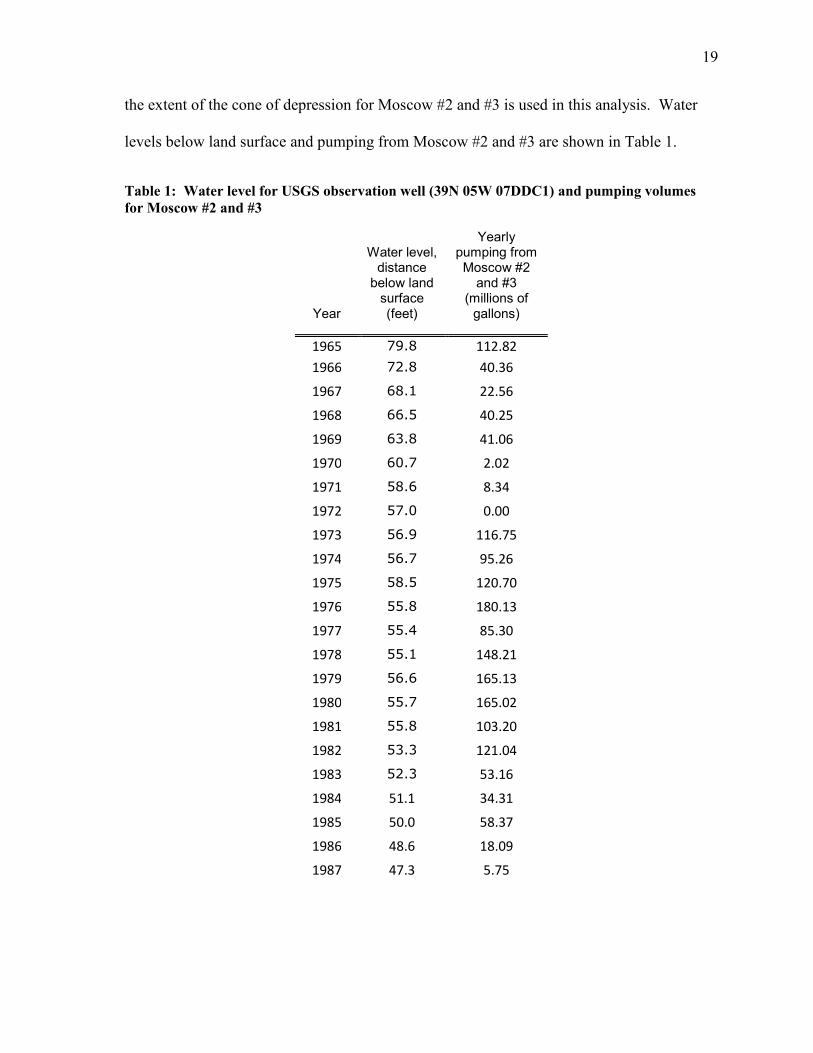
19

the extent of the cone of depression for Moscow #2 and #3 is used in this analysis. Water

levels below land surface and pumping from Moscow #2 and #3 are shown in Table 1.

Table 1: Water level for USGS observation well (39N 05W 07DDC1) and pumping volumes for Moscow #2 and #3

Year

Water level, distance below land surface (feet)

Yearly pumping from Moscow #2 and #3

(millions of gallons)

1965 79.8 112.82 1966 72.8 40.36

1967 68.1 22.56

1968 66.5 40.25

1969 63.8 41.06

1970 60.7 2.02

1971 58.6 8.34

1972 57.0 0.00

1973 56.9 116.75

1974 56.7 95.26

1975 58.5 120.70

1976 55.8 180.13

1977 55.4 85.30

1978 55.1 148.21

1979 56.6 165.13

1980 55.7 165.02

1981 55.8 103.20

1982 53.3 121.04

1983 52.3 53.16

1984 51.1 34.31

1985 50.0 58.37

1986 48.6 18.09

1987 47.3 5.75

20

The USGS observation well (39N 05W 07DDC1) was monitored from 1937 to 1987

when an obstruction in the well made it impossible to take further measurements. The

observation well is believed to have been outside of the influence of Moscow #2 and #3

during the recovery period of 1965 to 1987. If this assumption is correct, the water level

measurements would be free from the influence of pumping. If the USGS well were subject

to influence of pumping from Moscow #2 and #3, the measured change in water levels

would be greater than the actual change in the system. The resulting affect would cause

recharge rates to appear higher than they were.

The extent of the cone of depression described by Badon (2007) indicates that the

cone of depression is elliptical in shape. Badon (2007) indicates that transmissivity is

highest in the north-south direction because of lateral fractures acting as preferential

pathways. The illustration of the cone of depression depicted in Badon (2007) shows an

elliptical cone of depression with the long axis running east-west and the north-south

boundaries at the Bond and Brandt wells. However, with transmissivity highest in the north-

south direction, the cone of depression should be elliptical with the long axis running north-

south from the Bond to the Brandt wells. For this analysis, three different areas are used to

calculate the recharge: circular; elliptical, long axis running north-south; elliptical, long axis

running east-west (Figure 3). The areas were calculated using distances measured with

Google Earth.

Figure

Figure 3 shows the approximate areas of the different cone of depression scenarios: blue,

small ellipse; green, large ellipse; yellow, circular.

Aquifer tests #1 and #2 conducted by Badon were used to estimate

values for the Wanapum. The average of the storativity values is 0.04 and is used for this

analysis. All the values for storativity fall within the expected range for an unconfined

aquifer (0.01 to 0.3) suggesting that the Wanapum aquifer system is unconfined in the

vicinity of Moscow #2 and #3

(GoogleEarth.com, 15 Feb. 2009)

Figure 3: Cone of depression scenarios


small ellipse; green, large ellipse; yellow, circular.

Aquifer tests #1 and #2 conducted by Badon were used to estimate a range of

The average of the storativity values is 0.04 and is used for this


to 0.3) suggesting that the Wanapum aquifer system is unconfined in the

f Moscow #2 and #3(Freeze and Cherry, 1979).

21


a range of storativity

The average of the storativity values is 0.04 and is used for this


to 0.3) suggesting that the Wanapum aquifer system is unconfined in the

22

The storage equation is used for this analysis and is presented below

� � � � (3-1)

The change in storage is equal to inflow minus the outflow

� � � � (3-2)

The change in storage is equal to the change in water level multiplied by the affected area

(cone of depression) and the storativity. The recharge to the system is the inflow and

outflow is assumed to be only pumping. Recharge is the net gain or loss to the aquifer and

can be solved for directly.

�� (3-3)

The recharge determined with this method is a combination of the total volume pumped plus

the change in water level multiplied by the area of influence of the well and the storativity.

3.2 Expert Elicitation

In this work, the prior probabilities for the individual studies was elicited by having a

set of experts assess the recharge estimates and the methods used to obtain them, as

described in the Literature Review. The expert assigns a weight for each estimate. The

prior probability obtained for each estimate is used to calculate a single weighted recharge

estimate and variance.

Experts in the field of hydrology were contacted to determine if they would be

willing to contribute their time for an elicitation process. The experts contacted were Dr.

23

Kent Keller, Dr. Mike Barber, Dr. Dale Ralston, Dr. Fritz Fiedler, Dr. Gary Johnson, Dr. Jan

Boll, Dr. Tim Link, Dr. Paul McDaniel, Dr. Jerry Fairley, and Dr. Jim Osiensky, and Steve

Robischon; they represented faculty from the University of Idaho, Washington State

University, the Palouse Basin Aquifer Committee (PBAC), and a private consulting firm.

Three of the experts are considered to be generalists and the remaining eight are specialists.

The experts were given information on BMA, summaries and abstracts of the twelve studies

considered, and a set of elicitation issues and questions. The elicitation addressed four

issues:

• Is the set of methods used to determine recharge to the Wanapum aquifer complete?

• What are the plausibility ranks (1 to 12, least to most plausible) for each of the

studies?

• What is the probability value that best represents the confidence you would place in

each of the recharge studies?

• What value would you assign to the variance for each of the recharge studies?

Six general questions and five specific questions were asked to each expert. The questions

are:

General Questions Regarding All Studies

1. Is the set of methods used to estimate recharge complete? (yes, no) If your answer is “no” specify additional plausible methods for recharge estimation.

2. Which study do you believe gives the best predictions of recharge?

24

3. What probability range (e.g., 40-60%) reflects the degree of belief that the study named in #2 is the best?

4. Which study do you believe gives the worst predictions of recharge?

5. What probability range reflects your degree of belief that the study named in #4 is the worst?

6. What are the study ranks in terms of plausibility? Studies are ranked from 1 (least plausible) to 12 (most plausible). Different studies may have the same rank, indicating that the expert has the same degree of belief as to the plausibility of both studies.

Study Specific Questions

1. To what degree is the study based on solid physical principles? (high, intermediate or low)

2. Is the study contrary to any of your knowledge or experience? (yes, no) If “yes” please specify the reason.

3. Is the study qualitatively comparable to the others in terms of plausibility? (yes, no) If “no” please specify the reason.

4. What is the probability value that best represents the confidence you would place on this recharge study? Different studies may have the same rank, indicating that the expert has the same degree of belief as to the plausibility of both studies.

5. Given your knowledge of the method used, what variance, expressed in percent, would you expect from this method?

25

This elicitation closely followed the method recommended by Ye et al. (2008), with

some variation in the recommended training period. A day long training period was

recommended by Ye et al. (2008), but due to the time constraints involved, the experts were

provided information on BMA and the recharge study summaries for them to review on their

own. As discussed later, time was an issue for some experts even with requirements less

than those recommended in the current literature.

The twelve studies included in the elicitation had recharge estimates that ranged

from 0.2 (in/yr) to 4.8 (in/yr). The method and estimate of recharge for each study is shown

in Table 2. More detailed summaries are available in the Appendix.

26

Table 2: Studies Included in the Expert Elicitation

Study Method Estimate of Recharge (in/yr)

Stevens (1960)

Mass balance

1.2

Foxworthy and Washburn(1963)

Mass balance

0.9

Barker (1979)

Darcy’s Law

0.94

Smoot and Ralston (1987)

USGS Daily Deep Percolation Model

3.6

Bauer and Vaccaro (1990)

USGS Daily Deep Percolation Model

2.8

Johnson (1991)

One dimensional infiltration model (LEACHM)

4.2

Muniz (1991)

One dimensional infiltration model (LEACHM)

2.1

Baines (1992)

Hill method and zero change method

1.06

O’Brien (1996)

Chloride mass balance

0.98

O’Geen (2004)

Chloride mass balance

0.17

Dungel (2007)

Mass balance

1.8

Reeves (2009)

Storage equation

4.8

27


Bayesian model averaging is used to combine recharge estimates based on their prior

probabilities and determine an average recharge rate and corresponding degree of

uncertainty. BMA is a statistical approach for combining models which provides a

description of the uncertainty that accounts for between-model and within-model variances

(Duan et al., 2007). Let recharge �� be the quantity to be forecast and M = [M1, M2,….., Mk]

the set of all models considered, and D is the set of observation data. The probability

density function of the BMA probabilistic prediction of y can be represented by

�� ! � " ��#$%& '$��! ( �$��'$�) �! (3-4)

where �$��'$�) �! is the posterior probability of model prediction '$�being correct

given the observation data, D, also known as the likelihood of model '$�being correct. K is

the number of models considered. The posterior probabilities add up to one,

" ��#$%& '$��! � * , and they can be viewed as weights on individual models. The

posterior probabilities are obtained using site observations and the prior probabilities.

��'$�� ! +,-./01

2�#34567�85�!" ,-./01

2�#3496:9;1 7�89�!

(3-5)

The posterior probability is ��'$�� !; KIC is the Kayshap information criterion which uses

calibration data, number of parameters, and a weight matrix and sensitivity matrix; ��'$�! is

the prior probability of '$�(Ye et al., 2008). The posterior probability is the prior

probability conditioned on observation data from the different models. The studies that have

been examined for this analysis do not provide the luxury of reams of observation data and

more discussion on the Kayshap criterion is neither necessary nor applicable because the

28

prior probabilities are used in place of the posterior probabilities. The posterior probability

is the prior probability conditioned by observation data. The prior probabilities are

subjective values, whereas the posterior probability is a modification of the subjective value

based on a given models consistency with available data (Ye et al., 2008). Modifying the

priors on the observation data reduces the uncertainty associated with a given probability

estimate. Using the priors in place of the posteriors will mean that the uncertainty estimate

is conservative. For example, the estimate for uncertainty using prior probability may be

60%, but if more information were available to modify the prior probability the uncertainty

might be reduced to 50%.

The Bayesian estimate of the mean and variance of �� is given by,

�<�� = � " �<��) '$�=#$%& ��'$�� ! (3-6)

>��<�� = � " >��<��) '$�=#$%& ��'$�� ! (3-7)

�" ��<��) '$�=#

$%& � �<�� =!?��'$�� !

�<�� = is the mean and >��<�� = is the variance of �� under model Mk because of the

uncertainty associated with model Mk.

In essence the BMA prediction is the average output of the individual model weighted

by the likelihood that the individual model output is correct given observation data D (Duan

29

et al., 2007; Raferty et al., 2003). The variance of the BMA prediction is a measure of the

uncertainty that accounts for both between-model variance and within-model variance.

30

Chapter IV

Results

4.0 Recharge Estimation Using Historical Data

A five year moving average of both water level change and pumping was used to

determine recharge using equation 3-3. The results are shown in Table 3.

Table 3: Five year moving averages of water level, pumping, and recharge

Year

Water level,

distance below land

surface (feet

Change in

water level (feet)

Five year

moving average

of change in water

level

Yearly pumping

from Moscow #2 and

#3 (millions

of gallons)

Five year moving

average of pumping

from Moscow

#2 and #3 (ft3)

Recharge, circular cone of

depression (in/yr)

Recharge, small

ellipsoid cone of

depression (in/yr)

Recharge, large

ellipsoid cone of

depression (in/yr)

1964 83.9 1965 79.8 4.06

112.82

1966 72.8 7.06

40.36 1967 68.1 4.63 4.02 22.56 6888886 4.0 5.0 2.9

1968 66.5 1.66 3.83 40.25 3919559 3.0 3.6 2.4 1969 63.8 2.66 2.82 41.06 3061452 2.3 2.7 1.8 1970 60.7 3.14 2.23 2.02 2456831 1.8 2.2 1.4 1971 58.6 2.02 1.91 8.34 4506849 2.3 2.9 1.5 1972 57.0 1.65 1.42 0.00 5959355 2.5 3.4 1.5 1973 56.9 0.08 0.43 116.75 9139926 3.0 4.3 1.5 1974 56.7 0.23 0.57 95.26 13744032 4.5 6.5 2.2 1975 58.5 -1.85 0.31 120.70 16030179 5.0 7.4 2.4 1976 55.8 2.72 0.37 180.13 16873441 5.3 7.8 2.5 1977 55.4 0.37 0.02 85.30 18745957 5.7 8.4 2.6 1978 55.1 0.36 0.57 148.21 19933626 6.4 9.2 3.1 1979 56.6 -1.48 0.00 165.13 17871714 5.5 8.0 2.5 1980 55.7 0.90 0.42 165.02 18829492 5.9 8.7 2.8 1981 55.8 -0.13 0.55 103.20 16282179 5.2 7.6 2.5 1982 53.3 2.46 1.10 121.04 12776337 4.4 6.3 2.3 1983 52.3 1.02 1.13 53.16 9918064 3.6 5.0 1.9 1984 51.1 1.26 1.43 34.31 7637062 3.0 4.1 1.8 1985 50.0 1.05 1.21 58.37 4547236 2.0 2.6 1.2 1986 48.6 1.37 1.26 18.09 Average 4.0 5.6 2.1 1987 47.3 1.34 1.25 5.75 recharge

31

A five year moving average helps to reduce the effects of yearly variations in pumping

and recharge. The estimates for recharge are presented in Table 4.

Table 4: Average recharge for the Wanapum aquifer system

Average recharge,

circular cone of depression

(in/yr)

Average recharge, small ellipsoid

cone of depression (in/yr)

Average recharge, large ellipsoid cone of depression (in/yr)

4.0 5.6 2.1

The recharge rates vary from 2.1 in/yr to 5.6 in/yr highlighting the importance of

conceptual uncertainty associated with this method. The range of recharge rates is a direct

result of the variation of area in the size of the cone of depression. The cone of depression

from Badon (2007) is elliptical in shape with the long axis running east-west which would

be indicative of high east-west transmissivity. This shape is a result of the lack of data

points in the vicinity of Moscow #2 and #3. The program used to generate the cone of

depression interpolated between known points. The shape of the cone of depression is likely

somewhere between the circle and the small ellipse, based on the pump tests done by Badon

(2007) which indicate a high north-south transmissivity and an idealized circular cone of

depression, an average of which yields a recharge rate of 4.8 (in/yr).

Recharge to the Wanapum may be directly controlled by the degree of

compartmentalization which exists. Some compartments may experience high rates of

recharge while other may receive little to no recharge due to preferential pathways and

32

geologic features. Preferential flow paths play a large role in defining the shape of the cone

of depression. The high north-south transmissivity described by Badon (2007) is likely the

result of lateral fractures which provide preferential flow paths for both recharge and

pumping. The cone of depression intersects Paradise Creek which is a potential source of

concentrated recharge in the vicinity of Moscow #2 and #3. If this were the case, Paradise

Creek could act as a constant head boundary and very little drawdown would be experienced

in that vicinity.

The volume of municipal water pumped by the City of Moscow has a five percent error

associated with it. The flow meters used by the city are calibrated to within five percent and

regularly maintained to ensure high accuracy (email communication with Tom Scallorn).

Water level measurements for the USGS observation well were taken with either a steel or

electronic tape. The error in these measurements at a maximum would be 0.1 ft (Nielsen

and Nielsen, 2006). These sources of error pale in comparison to the conceptual

uncertainty. At a minimum the uncertainty would be five percent with a maximum of fifty-

six percent based on the ratio of the large ellipse cone of depression scenarios to the average

area of the circular and small elliptical cone of depression.

The average recharge in the vicinity of Moscow #2 and #3 determined by this analysis is

97 million gallons per year. The use of Moscow #2 and #3 as a municipal supply ramped up

in 1991 and averaged 203 million gallons per year through 2005, by comparison the period

from 1967 to 1990 averaged 72 million gallons per year. Approximately two thirds of the

33

water pumped from the Wanapum aquifer system is from Moscow #2 with the remainder

from Moscow #3. Since pumping ramped up in 1991, there has been a slight decline of

water levels in Wanapum aquifer system, indicating that pumping exceeds recharge and the

current rate of pumping is not sustainable long term.

4.1 Expert Elicitation

Eight experts participated in this study, and individual expert names are not associated

with their responses herein. The elicitations were conducted via personal interview over a

period of two weeks. A meeting was set up with each expert and the elicitation was

conducted in one to two hours depending on the depth of discussion for each of the

individual studies, and the results documented on a questionnaire during the personal

interview. The methods and issues regarding each study were discussed and the expert

answered the general and study specific questions. The prior probability estimates for each

individual study were aggregated using an arithmetic mean. An arithmetic mean was used

because other iterative methods of aggregation are more time intensive, and the experts

volunteering their time had a limited amount available for this exercise. Iterative methods

also give very similar results to the arithmetic mean. Ye et al. (2008) used an iterative

aggregation method that required the experts to place averaging weights on their own

judgments as well as the other expert’s judgments. Upon learning the other expert’s

assessments, expert A could change his probability estimate. The process would eventually

converge on a single probability estimate for a given study. Ye et al. (2008) found that the

difference in aggregating model probabilities using an arithmetic mean versus an iterative

34

method was only one percentage point for two of the five studies. The three remaining

studies had the same probability regardless of the aggregation method.

The experts chose which study they felt was the best and the worst, and estimated the

prior probabilities and the variance of the twelve studies based on their experience in

hydrology and their knowledge of the basin. Figure 4 shows the range of prior probabilities

for the individual studies.

Figure 4: Prior probability distribution of recharge studies

The figure shows the prior probability estimated by each expert for each of the studies

considered. This prior probability represents the expert’s confidence that the study estimates

a reasonable recharge rate. The prior probability estimated by the experts for Stevens (1960)

0

0.1

0.2

0.3

0.4

0.5

0.6

0.7

0.8

0.9

1

Prob

abili

ty Expert 1

Expert 2

Expert 3

Expert 4

Expert 5

Expert 6

Expert 7

Expert 8

35

varied from 0.1 to 0.8. Similarly, the prior probabilities can be seen to vary for each of the

individual studies. Johnson (1991) and Muniz (1991) have the lowest prior probabilities

which vary from 0.1 to 0.65. These two vadose zone studies were conducted near Pullman,

WA and were consistently ranked as giving the worst predictions of recharge for the

Wanapum aquifer system. Several experts reasoned that the vadose zone studies estimate

recharge to the loess, but because of lateral flow paths they do not give an accurate measure

of the recharge reaching the Wanapum aquifer system. There is also significant

heterogeneity in the Basin, and assuming soil properties are consistent between Moscow, ID

and Pulllman, WA is likely incorrect. The two studies with the highest prior probability

distributions are Dungel (2007) and Reeves (2009) which vary from 0.4 to 0.85 and 0.4 to

0.9. Reeves (2009) and Bauer and Vaccaro (1990) were ranked by the experts as giving the

best predictions of recharge. The reasoning was that Reeves (2009) directly estimated

recharge to the Wanapum aquifer system from historical water level and pumping data. The

USGS was ranked high because of their reputation of high quality work and the effort put

into addressing uncertainty through a sensitivity analysis. There was not the same

consensus among the experts when ranking the best study as there was when ranking the

worst study.

The aggregated prior probabilities for the individual studies can be seen below in

5. The prior probabilities were aggregated using an arithmetic mean.

Figure 5: Aggregated

The graph shows the

Three observations are made based on

lowest prior probabilities of 0.29 and 0.30. Stevens (1960), Foxworthy and Washburn

(1963), Barker (1979), Smoot and Ralston (1987), Bauer and Vaccaro (1990), Baines

(1992), O’Geen (1996), and O’Brien (2004) have

0.52. The third observation

and Reeves (2009). They have probabilities of

0.00

0.10

0.20

0.30

0.40

0.50

0.60

0.70

0.80

0.90

1.00

Prob

abili

ty

The aggregated prior probabilities for the individual studies can be seen below in

probabilities were aggregated using an arithmetic mean.

: Aggregated prior probabilities of recharge studies

prior probabilities for the 12 studies varying from

observations are made based on figure 5. Johnson (1991) and Muniz (1991) have the

probabilities of 0.29 and 0.30. Stevens (1960), Foxworthy and Washburn


992), O’Geen (1996), and O’Brien (2004) have prior probabilities varying

observation is that two studies have higher prior probability, Dungel (2007)

and Reeves (2009). They have probabilities of 0.64 and 0.61 which is 0.13 a

36

The aggregated prior probabilities for the individual studies can be seen below in Figure

ing from 0.29 to 0.64.

. Johnson (1991) and Muniz (1991) have the

probabilities of 0.29 and 0.30. Stevens (1960), Foxworthy and Washburn


ing from 0.38 to

probability, Dungel (2007)

0.64 and 0.61 which is 0.13 and 0.09 higher

than the next most likely study, O’Geen (2004). The spread in probabilities indicates the

range of likelihoods of the studies. Experts also estimated the

expect from a given method, because there was not enough e

estimate the variance for the individual studies.

variance.

Figure 6: Aggregated variance of recharge

0

10

20

30

40

50

60

70

80

90

100

Var

ianc

e (%

)


of likelihoods of the studies. Experts also estimated the sample variance

, because there was not enough existing data to quantitatively

estimate the variance for the individual studies. Figure 6 shows the distribution of the

: Aggregated variance of recharge studies

37


variance they would

quantitatively

distribution of the

38

The variance for the individual studies ranged from 49 % to 89 %. The high range of

variance indicates that a particular method will generate substantially different numbers

when applied in different studies. The range in the variance indicates that the experts

believed that the variance for some methods was less than others.

In conducting the elicitation interviews, several issues regarding time, scale, the

definition of recharge, and applicability of the studies were brought up by the experts. All

of the experts expressed that it was difficult to place probabilities on the individual studies

and indicated that they could give better estimates if they had more time and resources to

devote to the elicitation. At the time this work was conducted, most of the experts were full

time faculty at the UI and WSU and had limits on the amount of time they could give to the

elicitation. Recognizing that the experts were volunteering their time, the time requirements

were kept at a minimum thought necessary to obtain useful data for BMA. It would not be

feasible to expect the experts to give large amounts of their time to a project for which they

are not funded to participate, neither could high participation be expected if the elicitation

required a large time commitment. The elicitation interviews averaged around an hour in

duration and the experts were given research material on the studies to review. The total

time put into the elicitation varied from about an hour and a half to three hours depending on

the expert. Several experts expressed concern about the time required, and two were reticent

to provide elicitation data because of their concern for providing quality information with

limited time.

39

The definition of recharge for this study had to be clarified during elicitation.

Recharge for this study is defined as deep percolation that reaches the Wanapum aquifer

system and would be available to the City of Moscow for municipal use. The experts

expressed that the studies did not all specifically address recharge to the Wanapum aquifer

system, and the recharge estimates in some of the studies may not pertain to the Wanapum

aquifer system. For instance, Johnson (1991) and Muniz (1991) used a one dimensional

analysis to estimate recharge through the loess; however, recharge to the loess may not be

indicative of recharge to the Wanapum aquifer system because fragipans in the loess inhibit

vertical infiltration and cause water to travel laterally. Scale was another issue brought up

by many experts. The scale of the different studies varied from basin wide to specific

locations. Investigations conducted by Reeves (2009), O’Geen (2004), Baines (1992),

Johnson (1991), and Muniz (1991) were site specific, but studies by Dungel (2007), O’Brien

(1996), Smoot and Ralston (1987), Bauer and Vaccaro (1990), Barker (1979), Foxworthy

and Washburn (1963), and Stevens (1960) had implications basin wide. Estimations that are

valid on a small scale may not be transferrable to a larger scale and vice versa. Estimates for

hydraulic conductivity can vary significantly when going from small to large scale (Brooks

and Boll, 2004).

The complexity of the studies was addressed by many of the experts. The general

consensus was that the studies using the simplest approach to directly estimate the recharge

were better than the more complex studies that didn’t directly address recharge. The experts

also indicated that the set of recharge methods was not complete and some type of tracer

study should be conducted in the Basin.

40


The aggregated prior probabilities determined from the expert elicitation are

weighted so that they sum to one and used in equation 3-6 and equation 3-7 to give the

Bayesian estimate of the mean and variance. The weighted prior probabilities are shown in

Figure 7.

Figure 7: Weighted prior probabilities of individual studies

The weighted prior probabilities ranged from 0.05 for Johnson (1991) and Muniz

(1991) to 0.12 for Dungel (2007). The prior probabilities are used to calculate both the

BMA estimate and the variance. The variance takes into account both the within model

Stevens (1960), 0.08

Foxworthy and Washburn (1963),

0.08

Barker (1979), 0.07

Smoot and Ralston (1987), 0.09

Bauer and Vaccaro (1990), 0.08

Muniz (1991),

0.05Johnson (1991),

0.05

Baines (1992), 0.09

O'Brien (1996), 0.09

O'Geen (2004), 0.09

Dungel (2007), 0.12

Reeves (2009), 0.11

variance and the between model variance. Figure 8 shows the within and between model

variance for each study.

Figure 8: Variance within and between studies

The variance for each study is summed to determine the total

in2/yr2. Reeves (2009) has the largest variance of all the studies. This is a result of the

between model variance which adds the square of the difference between the BMA estimate

and the individual study estimate.

on assumptions about the cone of depression from Moscow #2 and #3. If the cone of

depression is larger than assumed, the recharge

0.000.100.200.300.400.500.600.700.800.901.001.101.201.30

Var

ianc

e (in

2 )


: Variance within and between studies

each study is summed to determine the total variance

has the largest variance of all the studies. This is a result of the

variance which adds the square of the difference between the BMA estimate

and the individual study estimate. The average from Reeves (2009) is 4.8 in/yr and is based


ssion is larger than assumed, the recharge volume would be distributed over a larger

41


variance, which is 3.4

has the largest variance of all the studies. This is a result of the

variance which adds the square of the difference between the BMA estimate

The average from Reeves (2009) is 4.8 in/yr and is based


volume would be distributed over a larger

42

area and would result in a smaller aerial estimate and a smaller variance. For example if the

recharge were 3.0 in/yr the variance would be 2.6 in2/yr2 instead of 3.4 in2/yr2. This further

highlights the importance of the conceptual assumptions in the method described previously.

The results of BMA are shown in Table 5, with different ways of quantitatively expressing

uncertainty.

Table 5: Results of Bayesian Model Averaging

Bayesian Model Averaging results

Recharge estimate (in/yr)

Variance (in/yr)2

Standard Deviation (in/yr)

95% CI (in/yr)

2 3.4 1.8 2 ± 3.6

The estimate of recharge using BMA is 2.0 inches per year with a variance of 3.4

in2/yr2. The variance is the quantitative measure of uncertainty in this estimate and takes

into account the variance within the individual studies as well as the variance between the

studies (Duan et al., 2007). Most studies that do assess uncertainty only estimate the within

model variance. Figure 9 shows the probability distribution of recharge with the standard

deviation, variance and 95 % confidence interval, assuming a normal distribution.

43

Figure 9: Probability distribution of recharge (not to scale)

Converting the variance to standard deviation, the recharge estimate would be 2.0 ±

1.8 inches per year. The 95 % confidence interval would be 2 ± 3.6 inches per year. As is

typical (Ye et al., 2008), it is assumed in the analysis that the data are normally distributed.

However, the physical lower bound for recharge is zero thus recharge is not rigorously

normally distributed.

The estimate of uncertainty here is higher than seen in individual studies because it

additionally incorporates the between study variance. The recharge estimate was derived

0

0.1

0.2

0.3

0.4

0.5

0.6

-2.5 -2 -1.5 -1 -0.5 0 0.5 1 1.5 2 2.5 3 3.5 4 4.5 5 5.5 6 6.5

Prob

abili

ty

Recharge (in/yr)

Mean

SD

VarVar

SD

95% CI95% CI

44

using studies that estimated recharged aerially as well as by total volume. All of the

recharge numbers were converted to aerial estimates for use in BMA. The estimate of

recharge determined with BMA is applicable over the recharge area of the Wanapum in the

Moscow sub-basin. A volume of recharge could be determined once the recharge area has

been delineated.

This research differs from the expert elicitation studies discussed in the literature in

that the models to estimate recharge in the Palouse Basin were not available to generate data

or new scenarios. The studies discussed in the literature review had available several

models to generate output data used to condition the prior probabilities. The situation in the

Palouse Basin represents a situation where observation data and model output data are more

limited, but conclusions and results must be drawn despite limited data.

45

Chapter V

Social and Scientific Uncertainty and Implications on Decision

Making

5.0 Scientific and Social Uncertainty

Physical and social sciences, though very different, complement each other. A

broader understanding of water resource management within the Palouse Basin is facilitated

when both physical and social science are concurrently considered. One uniting theme in

both the physical and social scientific research on the Palouse Basin is uncertainty, which is

a factor affecting decision making. In order to satisfy the interdisciplinary requirement of

the Water Resource Program this chapter is co-author this chapter with Katherine Bilodeau,

another Master’s candidate in the Water Resources Program whose research focused on

social uncertainty in the Palouse Basin. Minor differences are a result of different graduate

committees. The following co-authored chapter addresses the following question: What are

uncertainties of the social and physical systems of a water resource and how might these

combined variables affect decision making in the Palouse Basin?

In the physical hydrologic system, uncertainty is present as parameter uncertainty

and conceptual uncertainty. Parameter uncertainty is the mathematical error that would

result from calculating a hydrologic parameter such as streamflow, precipitation, or other

parameters in the water budget. Conceptual uncertainty results because the actual

hydrogeologic structure, stratigraphy and bounds of an aquifer system cannot be perfectly

represented nor even understood. In the social sciences that focus on the Palouse Basin,

uncertainty can have multiple inferences. Uncertainty can simply be that the stakeholders’

46

knowledge, perceptions, beliefs, and opinions are unknown. Response behavior of

individuals is another social aspect of uncertainty.

5.1 Decision Making Approaches

Several approaches to decision making can be employed for natural resource

management, and these approaches can rely on a combination of criteria on which to base

decisions and system feedback. One important component of decision making is the

identification of who has the authority to make the decision. When multiple decision

making entities are involved, jurisdiction is a boundary to the subsequent decision making

strategy (Holecheck et al, 2003). Federal agencies, such as the U.S. Environmental

Protection Agency and the U.S. Fish and Wildlife are not bound by geographical jurisdiction

but by purpose, i.e. protection of environmental components. On the other hand, state,

county, and municipal agencies are limited by their political jurisdiction. The overlap of

political and environmental jurisdictions in regards to a natural resource obviously

complicates and limits decision-making processes.

The first approach for decision makers is the ever-present option to do nothing, or to

maintain the status quo. If the status quo is maintained, users do not change behavior in

resource use or allocation. No change in resource use means nothing new is risked, nothing

new is gained, and nothing new is lost. However, choosing to “do nothing” does not mean a

decision has not been made. Maintaining status quo regarding resource use is a passive

decision to continue using the resource without change, which may have adverse effects. If,

for example, the status quo is resource harvest (a take of the resource faster than the physical

47

system’s ability to recharge the resource), then a decision to “do nothing” will ultimately

result in complete resource depletion.

The alternative to the passive decision to “do nothing” is to make an active decision

using one of several criteria and approaches. Social order in a natural resource use follows a

balance of three basic criteria identified by Firey (1960): what is ecologically possible, what

is socially acceptable, and what is economically feasible. Loomis (2002) added two criteria

to Firey’s essential criteria: 1) operational practicality; and 2) distributional equity among

the current population/between present and future generations. Although not every criterion

needs to be addressed with a natural resource decision, sustainable management of a

particular natural resource use will balance all of the criteria (Firey, 1960; Loomis, 2002).

Past management or decision making approaches have relied simply on historical

trends or what has worked using the best current information at the time of the decision

(Montgomery, 1995; Johnson, 1999). These decision making approaches suggest that

decision making is a one-time event that may have a permanently altered effect on the

situation. Although a decision can permanently alter a situation and have unintended

consequences, decision making in the face of a natural resources dilemma is not necessarily

a one-time occurrence, more developed approaches reflect that of management reactions to

previous decisions in a continual manner. Decision making can be a process of feedbacks

and successive decisions referred to as “monitor and modify” (Johnson, 1999). “Monitor

and modify” uses decision feedback to gain knowledge (or reduce uncertainty) about a

variable and adapts with subsequent decisions that reflect the increased knowledge of the

system.

48

In the 1970s, this “monitor and modify” evolved to what is now known as adaptive

management (Holling, 1978). Although this new type of management has been applied to

different ecosystems and the resulting management classified under other names, i.e.

watershed analysis (Montgomery et al., 1995)), the philosophies and principles have

fundamentally identical components, which enables the classification of this approach into

one specific category. Adaptive management functions on the premise that, although a

system may not be understood with absolute certainty, the process of involving stakeholders

and responding to the constant feedback of new knowledge will enable better overall

understanding and benefit the guidance of further decisions (Montgomery 1995; Lee, 1999;

Johnson, 1999). A guiding philosophy in this management paradigm integrates social and

biological needs from the beginning in order to support decision making processes and lead

to an increased likelihood of successful management implementation (Montgomery, 1995).

In essence, adaptive management further develops monitor-and-modify management with an

interdisciplinary approach; various stakeholder epistemologies come together, gaps in the

comprehensive knowledge are identified and become scientific questions, and management

adapts to the new knowledge found, incorporating it into future decision-making processes

(Holling, 1978; Lee, 1999; Montgomery, 1995; Johnson, 1999; POST, 2004; Kemmis,

2002).

The temporal decision to act “now” or “later” has become a component of decision-

making that may have notable effects. The resolve to wait for more or better information

and then make a decision (i.e. to decide “later”) is a strategy based on the concept of the

Precautionary Principle (PP). In its purest theoretical form, the PP requires evidence that the

proposed risk-taking decision will not adversely alter the present situation (Gollier and

49

Treich, 2003). However, this is not to suggest that absolute conclusive evidence is

necessary to make a decision involving risk; the premise of the PP looks at the intersection

between the cost of waiting to make a decision, and the gain of better information for a

presumably less risky decision at a later date.

The physical and social scientific factors unique to every resource management

scenario can contribute to which approach or combination of approaches are used. Multiple

decision making entities with overlapping jurisdictions may affect the priorities of the

criteria and affect processes within those approaches. These factors undoubtedly include the

particular nature of the social and physical uncertainties of each system.

5.2 Physical and Social Scientific Factors Affecting Decision Making Approaches

The science used to inform decision-making related to water resource problems can

take various forms, such as streamflow hydrographs, well observation data, pumping data,

flood exceedence probability, and hydrogeologic models. Depending on the complexity of

the problem, the science to inform the decision makers may require that measured data such

as streamflow or ground water elevations be incorporated into a model of the system. The

challenge of modeling is to understand how the system works and reduce the uncertainty

associated with model output. Reducing the uncertainty provides decision makers with

better information when making a decision that involves legal, social, and scientific

complexities. The decision to act based on scientific information can be reduced to a single

parameter, uncertainty. Reducing the uncertainty in the physical system may necessitate

action due to legal or social constraints.

50

Social factors that generally affect decision-making include what groups know about

the resource, whether groups involved with resource harvest are willing to cooperate; the

level of uncertainty involved in the system; and the social or political response to a

management decision.

Natural resource management scenarios can sometimes be classified as a social

dilemma. A social dilemma is the junction between unsustainable use and the self-interest

vs. collective interest of the resource users was. It was initially described by biologist Garett

Hardin in his article The Tragedy of the Commons (1968), and further developed by Dawes

in 1980 (Biel and Garling, 1995; Roch and Samuelson, 1997). Dawes (1980) established

two defining characteristics for a social dilemma: (1) the social payoff is higher to users who

choose not to cooperate and harvest according to their self-interest, in other words, users

who defect; and (2) the collective payoff of users who unanimously choose to act in the

collective interest, or to cooperate, is higher than if all users defect. The preference to act

individualistically or to cooperate is a social value orientation (Messick and McClintock,

1968). This orientation, formed by the willingness of individuals or groups to cooperate,

can dictate which decision-making strategy is employed, as an approach such as adaptive

management is not conducive to defecting individuals/groups.

Value orientations affect decision-making in terms of harvest and uncertainty as

well. Experimental research has consistently identified that resource users who cooperate

(act in the collective interest), harvest at a significantly lesser rate than their defecting

counterparts (Roch and Samuelson, 1997; Kramer et al., 1986; Liebrand, 1984; Loomis et

al., 1995). Roch and Samuelson (1997) found that in resource scenarios of higher

51

uncertainty groups or individuals acting in the collective interest maintained or decreased

their harvests while defectors tended to increase harvest rate.

Another social factor that affects decision-making is the public or political response

to a decision. When the political or social responses are the first concern, it is not

uncommon for a decision to be to “do nothing” (Johnson, 1999). The PP may further feed

into politics affecting the approach by losing focus of the true issue or using system

uncertainty to postpone a decision pending further information (POST, 2004).

5.3 Uncertainty and Decision Making

Decision making can take place under any level of uncertainty. Understanding the

level of uncertainty and the range of decision alternatives available is more likely to

contribute to effective decision making than attempting to narrow uncertainty in the science

or the decision alternatives (Pielke and Conant, 2003). Scientists and decision makers often

mean different things when they seek to “reduce uncertainty”. Scientists may be seeking to

reduce the uncertainty in the understanding of a complex system while the decision maker is

seeking to reduce uncertainty in the decision outcomes (Pielke and Conant, 2003). When

scientists seek to inform decision makers of new science it is vitally important for them to be

on the same page when they are attempting to reduce uncertainty. Both the scientist and

decision maker must understand that uncertainty does not prevent decision making, but

gives a basis for choosing between several alternatives and determining if additional data is

are needed (Reckhow, 1994).

52

5.4 Palouse Basin

True to water resource management everywhere, the political overlay of the

hydrogeology in the Palouse Basin is distinct and unique. The basin underlies several cities

and is encompassed primarily by two counties, Latah County in Idaho and Whitman County

in Washington (Larson et al., 2000). Water management is governed separately by each

state with federal government considerations. In Idaho, the Idaho Department of Water

Resources (IDWR) manages Idaho surface and groundwater (IDWR, 2008). The state water

agency in Washington is the Department of Ecology (Washington Department of Ecology,

2008). As discussed earlier, authority is an integral component to decision making, and the

overlapping jurisdictions of water management in the Palouse (i.e. the state authorities and

municipal authorities) complicate water resource management in the Palouse Basin on a

fundamental level.

Falling ground water levels have been an issue in the Palouse Basin for the last fifty

years. The first response to address falling ground water levels in the Moscow sub-basin

was to drill deeper wells and bypass the shallower Wanapum aquifer. Water levels in the

deeper Grande Ronde aquifer system have decreased at a fairly constant rate since it was

first developed in the late 1800s. In recognizing the need for both research and education of

the public and policy makers about Palouse Basin water resources, the Pullman-Moscow

Water Resources Committee (currently known as the Palouse Basin Aquifer Committee, or

PBAC) published the Ground Water Management Plan (1992). This document established

PBAC as an organization that plays a role in water resource management, develops a water

resource management plan, conducts and promotes studies of ground water resources, and

encourages public involvement in plan development through educational programs and

53

forums. However, it is important to note that PBAC has no decision-making authority, and

wording carefully reflects such in the expressly stated role of the Pullman-Moscow Water

Resources Committee:

The role of the COMMITTEE is to encourage ENTITIES to implement the PLAN. The COMMITTEE will also monitor the success of the ENTITIES in carrying out their action plans and achieving the goals of the PLAN. Each ENTITY will be expected to adopt an action plan, interfacing with the stated goals of the PLAN. The COMMITTEE will provide guidance related to water-use plans, conservation strategies relative to water use, implementation policies, and the preparation of local ordinances or zoning regulations (PMWRC, 1992)

In the Ground Water Management Plan, PMWRC (1992) also established the goal of

limiting aquifer pumping increases to one percent per year with changes in pumping rates

implemented by agreement of the cities of Moscow (ID) and Pullman (WA), the counties if

Whitman (WA) and Latah (ID), and the Universities of Idaho and Washington State. This

decision essentially maintained the status quo because growth in the basin has been one

percent per year.

Management decisions in the Palouse Basin likely have been constrained by several

factors. The scientific information about the Palouse Basin aquifers has been developed

incrementally over a period fifty years. Incremental changes in new science may not

motivate decision makers to change how they make decisions (Morss et al., 2005).

Additionally, decision makers are constrained by time, money, and resources and may be

constrained by federal, state, and local regulations from using new information. Such

constraints reduce decision maker’s motivation to learn to use new methods and scientific

information. A disconnect between the recommendations by PBAC and the decision

making process currently exists (personal communication Fritz Fiedler, 2009). The role of

54

PBAC is to guide decisions, however, if PBAC representatives are not fully facilitating two-

way communication between their organizations and the PBAC, the disconnect likely will

result in hindering or stalling the decision making process. Decision makers seeking new

scientific information often turn to scientists whom they trust and with whom they have a

long-term relationship with (Morss et al., 2005). To aid in the decision making process, the

studies that PBAC commissions must not just give general scientific knowledge to the

decision makers, but must generate data or information that applies to the decision at hand.

When the needs of the decision makers are clearly understood, then the studies conducted

can directly address those needs, both reducing uncertainty in the science and educating the

decision makers in the process. Finally, significant scientific and social uncertainty,

including the risk-taking that uncertainty creates in decision-making, have likely contributed

to slower changes with Palouse Basin aquifer management.

Uncertainty in the physical system has been an issue for decision makers in the

Palouse Basin. For example, in the Palouse Basin the primary source of municipal water is

the Grande Ronde aquifer system. Water level records show a steady decline of 1.5 to 2 feet

per year for the last several decades. It is uncertain if the Grand Ronde aquifer is receiving

recharge, and if the pumping is in excess of the recharge. If the mining of groundwater was

100% certain from a scientific perspective, then the decision to curtail or continue pumping

would be based on the legality of ground water mining (I.C. s 42-237a). The Wanapum

aquifer system receives recharge, but there is no consensus on the amount of recharge.

Estimates of recharge in the Basin range from 0.2 to 4.8 inches per year. Part of this thesis

addressed this issue by taking twelve studies that estimate recharge and using an expert

elicitation process to determine the probability that each recharge estimate is correct.

55

Bayesian Model Averaging (BMA) was used to combine the recharge estimates and

determine the mean and variance. The BMA estimate by Reeves (2009) helps to resolve the

uncertainty in recharge to the Wanapum aquifer by taking into account the conceptual and

parameter uncertainty, in a manner not done by previous estimates. Recharge was estimated

at 2.0 ± 1.8 inches per year, and this estimate provides a measure to analyze the Wanapum

aquifer system for sustainability and can be adapted as new information becomes available.

The expert elicitation process was very useful because it showed a consensus between

experts regarding the studies of recharge to the Wanapum aquifer system, and yielded an

estimate of uncertainty. It also highlighted the need to better understand the recharge area

and recharge mechanisms of the Wanapum aquifer.

A considerable amount of social uncertainty exists in the Palouse Basin as well.

Approximately 44 percent of residents surveyed in the Palouse Basin did not know the

origin of their household water, suggesting a need for outreach educating the public about

their water source (Bilodeau, 2009). Survey respondents also self-rated their awareness of

water-related organizations and knowledge about decision-making processes low. This

could potentially make decision-making riskier because public response to decisions would

subsequently present a higher degree of uncertainty. The public indicated a low knowledge

about water resource planning/decision-making that occurs in the basin, and the proportions

are alike between well owner and municipal water user groups. Well owners and municipal

water users have a moderately high concern for water resources on the Palouse, and perceive

some problems with the water planning/decision-making within the community. Most

importantly, 75 percent of survey respondents indicated interest in learning more. Although

public response to specific measures cannot be gleaned from some general results the survey

56

produced, the combination of an apparent need for education outreach, interest in learning

more, and perception of problems with decision-making create an environment where the

public might successfully help scientists and policy-makers in the decision-making process.

5.4 Summary

This chapter examined scientific uncertainty in social and physical disciplines, and

their coupled effects on decision-making. Uncertainty in the physical system affects our

understanding of recharge to the aquifer systems, and physical system uncertainty can delay

management decisions. Public perception, values, and responses to water resource

management decisions might influence policy-makers. Without physical certainty guiding

management decisions, and the public response unknown, decision-makers have incentive to

adopt a Precautionary Principle strategy. Waiting for more information, given the

uncertainty in physical and social science, is perhaps the least risky decision-alternative in

terms of physical system alteration and social response. However, there is a fine line

between waiting for more information and the decision to maintain the status-quo (“do

nothing”). An alternative that reduces the risk that maintaining the status quo assumes is the

implementation of conservation measures. Conservation of the resource will not adversely

affect the system and would serve as an interim measure while efforts are made to reduce

the social and physical uncertainty. Conservation could have economic impacts if

conservation measures curtailed economic growth in the region. These impacts must be

weighed when making a decision. Uncertainty does not (nor should not) completely

prevent decision making. Early involvement of scientists, managers, decision makers, and

the public in the decision making process enhances a comprehensive understanding of the

57

physical and social science components involved with the natural resource. It also gives

decision makers and managers the opportunities to gather the specific information they

would require to make an informed decision. The decision making approach best

encompassing the characteristics described above is adaptive management. Decision makers

could make the pro-active decision to conserve while waiting for better social and physical

science. New information could be input into the adaptive management scheme in which

physical science and social science complement each other in the decision making process

by bringing comprehensive understanding of complex natural resource management issues

together and providing knowledge for decision makers to proceed with management

decisions despite existing components of uncertainty.

58

Chapter VI

Conclusions and Recommendations

6.0 Conclusions

Bayesian Model Averaging appears to be a useful tool for recharge estimation. The

data for recharge in the Palouse Basin is not exhaustive and comes from somewhat disparate

sources, but through the use of BMA a combined estimate of recharge and the associated

uncertainty were determined. The expert elicitation process that was part of the BMA would

likely yield slightly better results if more time and resources were available for the experts to

engage in the elicitation process. However, this constraint will frequently be encountered in

real situations. Funding the experts for a portion of their time might be a way to enable

them to free up additional time to spend on the elicitation. In addition to the quantitative

benefits of the elicitation, there are qualitative benefits to be gained. The elicitation process

helped to identify areas that need further research such as a tracer type study. It also

identified which studies were most applicable for estimating recharge to the Wanapum

aquifer as well as those that were not. While not yet known, the expert elicitation process

may lend more credence to the BMA estimate and reduce controversy over which estimate

is best.

The estimate of recharge to the Wanapum aquifer system determined through BMA

was 2.0 ± 1.2 inches per year. This estimate takes into account the variance within the

individual studies as well as the variance between the studies and represents the

understanding and knowledge of professionals that are familiar with the Palouse Basin thus

giving more credence to the estimate. Quantifying the uncertainty as has been done in this

59

study gives decision makers a baseline from which to work from. The uncertainty can be

targeted for reduction or several decision alternatives could be developed based on the

uncertainty. The uncertainty does not prevent decision making but it provides a basis for

choosing between various alternatives. The management strategy best equipped to deal with

uncertainty is adaptive management which involves scientists, managers, decision-makers,

and the public. Adaptive management helps to bring a comprehensive understanding of

complex natural resource management issues together and provides knowledge for decision-

makers to proceed with management decisions despite existing components of uncertainty.

The BMA method is well-suited to adaptive management frameworks.

6.1 Recommendations for Additional Research

The experts identified a tracer study as being another valuable tool to address

recharge in the Palouse Basin. A tracer study would utilize injected tracers or human

generated tracers such as caffeine or pharmaceuticals that would be discharged from the

wastewater treatment plant. A tracer study could be used to identify possible recharge areas

to the Wanapum aquifer as well as the recharge rate.

An expert elicitation process and BMA might be useful to apply to the Grande

Ronde aquifer to quantify both the uncertainty and the recharge; however, less data are

available for the Grande Ronde. A similar expert elicitation process for the Grande Ronde

thus might better focus on conceptual recharge mechanisms rather than specific recharge

60

estimates. It would also help to identify areas that need further research as well as areas

where there is a consensus among the experts.

61

References

Badon, N. M., 2007, Implementation of a Groundwater Monitoring Program and Aquifer Testing in the Wanapum Aquifer System, Latah County, Idaho: Master of Science thesis, University of Idaho, Moscow, ID, 180 p.

Baines, C. A., 1992, Determination of Sustained Yield for the Shallow Basalt Aquifer in the Moscow Area, Idaho: Master of Science thesis, University of Idaho, Moscow, ID, 60 p.

Barker, R. A., 1979, Computer Simulation and Geohydrology of a Basalt Aquifer System in the Pullman-Moscow Basin, Washington and Idaho, United States Geoligical Survey, p. 119.

Bauer, H. H., and Vaccaro, J. J., 1990, Estimates of Ground-Water Recharge to the Columbia Plateau Regional Aquifer System, Washington, Oregon, and Idaho, for Predevelopment and Current Land-use Conditions, Tacoma, Washington, U. S. Geologic Survey, p. 36.

Biel, A., Garling, T. (1995). "The Role of Uncertainty in Resource Dilemmas." Journal of Environmental Psychology 15: 221-233. Bilodeau, K.A. (2009). “Pooling Our Water Resource Knowledge: The Effect of Public Knowledge, Concerns, Opinions, and their Related Dynamics on Water Resources.” Master’s Thesis, University of Idaho. Bush, J., 2005, The Columbia River Basalt Group of the Palouse Basin with Hydrological Interpretations, Western Latah County, and Eastern Whitman County, Washington, Moscow, Idaho, p. 111.

Cook, I. C., 1897, A Reconnissance in Southeastern Washington, U.S. Geologic Survey, p. 96.

Crosby, J. W., Chatters, R.E., 1965, Water Dating Techniques as Applied to the Pullman-Moscow Ground-Water Basin: Washington State University College of Engineering Bulletin, v. 296, p. 21.

Dawes, R.M. (1980). “Social Dilemmas.” Annual Review of Psychology 31: 169-193.

DeWispelare, A. R., Herren, L.T., Clemen, R.T., 1995, The Use of Probability Elicitation in the High-level Nuclear Waste Regulation Program: International Journal of Forecasting, v. 11, p. 5-24.

Douglas, A. A., Osiensky, James L., and Keller, C. Kent, 2007, Carbon-14 dating of ground water in the Palouse Basin of the Columbia River Basalts: Journal of Hydrology, p. 502-512.

Duan, Q., Ajami, N.K., Gao, X., Sorooshian, S., 2007, Multi-model ensemble hydrologic prediction using Bayesian model averaging: Advances in Water Resources, v. 30, p. 1371-1386.

62

Facheaux, S., Froger G. (1995). "Decision-making Under Environmental Uncertainty." Ecological Economics 15: 29-42.

Fairley, J. P., Solomon, Mark D., Hinds, Jennifer J., Grader, George W., Bush, John H., and Rand, Amber L., 2006, Latah County Hydrologic Charcterization Project.

Fealko, J. J., 2003, A Probabilistic Water Resources Assessment of the Paradise Creek Water shed. Master of Science Thesis, University of Idaho

Fiedler, F., 2009, Personal Communication, in M. Reeves, ed., Moscow, ID.

Firey, W. (1960). Man, Mind, and Land: A Theory of Resource Use. Glencoe, IL: Free Press.

Foxworthy, B. L., and Washburn, R.L., 1963, Ground Water in the Pullman Area Whitman County, Washington, p. 44.

Freeze, R. A., Cherry, J.A., 1979, Groundwater: Eaglewood Cliffs, NJ, Prentice-Hall Inc., 604 p.

Hardin, G. (1968). “The Tragedy of the Commons.” Science 162: 1243-1248.

Hernandez, H. P., 2007, Observations of Recharge to the Wanapum Aquifer System in the Moscow Area, Latah County, Idaho: Mater of Science thesis, University of Idaho, Moscow, ID, 131 p.

Hoeting, A. J., Madigan, D., Raferty, A.E., Volinsky, C.T., 1999, Bayesian Model Averaging: A Tutorial: Statistical Sciences, v. 14, p. 382-417.

Holechek, J.L., Cole, R.A., Fisher, J.T., Valdez, R. (2003). Natural Resources: Ecology, Economics, and Policy. Upper Saddle River, NJ: Prentice Hall.

Holling, C.S. (1978). Adaptive Environmental Assessment and Management. New York: Wiley.

Gollier, C., Nicolas, T. (2003). "Decision-Making Under Scientific Uncertainty: The Economics of the Precautionary Principle." The Journal of Risk and Uncertainty 27(1): 77-103. Idaho Code § 42-237a. URL: http://www.legislature.idaho.gov/statutesrules.htm Idaho Department of Water Resources. URL: http://www.idwr.idaho.gov/. Retrieved online March, 2008. Johnson, B.L. (1999). “The Role of Adaptive Management as an Operational Approach for Resource Management Agencies.” Conservation Ecology 3(2): 8. URL: http://www.consecol.org/vol3/iss2/art8/

http://www.consecol.org/vol3/iss2/art8/

63

Johnson, G. E., 1991, Estimating Groundwater recharge beneath different slope positions in the Palouse formation using a numerical unsaturated flow model: Master of Science thesis, Washington State University, Pullman, 111 p.

Jones, R. W., Ross, Sylvia H., 1972, Moscow Basin Ground Water Study, Moscow, ID, Idaho Bureau of Mines and Geology, p. 95.

Keeney, R. L., Winterfeldt, D., 1991, Eliciting Probabilites from experts in Complex Technical Problems: IEEE Transactions On Engineering Management, v. 38, p. 191-201.

Kemmis, D. (2002). “Science’s Role in Natural Resource Decisions.” Issues in Science and Technology (Summer): 31-34. Kramer, R.M., McClintock, C.G., and Messick, D.M. (1986). Social Values and Cooperative Response to a Simulated Resource Conservation Crisis.” Journal of Personality, 54(3): 576-592.

Larson, K. R., Keller, C. Kent, Larson, Peter B., and Allen-King, Richelle M., 2000, Water Resource Implications of 18O and 2H Distributions in a Basalt Aquifer system: Ground Water, v. 38, p. 947-953.

Lele, S. R., and Das, Abhik, 2000, Elicited Data and Incorporation of Expert Opinion for Statistical Inference in Spatial Studies: International Association for Mathematical Geology, v. 32, p. 465-487.

Lee, K. N. (1999). "Appraising Adaptive Management." Conservation Ecology 3(2): article 3. Liebrand, W.B.G. (1984). “The Effect of Social Motives, Communication, and Group Size on Behaviour in an N-person Multi-stage Mixed-motive game.” European Journal of Social Psychology 14: 239-264. Loomis, D.K., Samuelson, C.D. and Sell, J.A. (1995). “Effects of Information and Motivational Orientation on Harvest of a Declining Renewable Resource.” Society and Natural Resources 8: 1-18. Loomis, J.B. (2002). Integrated Public Lands Management: Principles and Applications to Ntaional Forests, Parks, Wildlife Refuges, and BLM Lands. New York: Columbia University Press.

Lum, W. E., Smoot, J.L., and Ralston, D.R., 1990, Geohydrology and Numerical Model Analysis of Ground-Water Flow in the Pullman-Moscow Area, Washington and Idaho, Tacoma, WA, U.S. Geologic Survey, p. 73.

Messick, D.M., and McClintock, C.G. (1968). “Motivational Bases of Choice in Experimental Games.” Journal of Experimental Social Psychology 4(1): 1-25

64

Montgomery, D.R., Grant, G.E., Sullivan, K. (1995). “Watershed Analysis as a Framework for Implementing Ecosystem Management.” American Water Resources Association, Water Resources Bulletin 31(3): 369-386. Morss, R. E., Olga V., , Downtown, M.W., Gruntfest, E. (2005). "Flood Risk, Uncertainty, and Scientific Information for Decision Making: Lessons from an Interdisciplinary Project." American Meteorological Society 86(1593-1601).

Muniz, H. R., 1991, Computer Modeling of Vadose Zone Groundwater Flux at a Hazardous Wast Site: Master of Science thesis, Washington State University, Pullman, 140 p.

Pielke, A. R., Conant, R.T. (2003). "Best Practices in Prediction for Decision Making: Lesson From the Atmospheric and Earth Sciences." Ecology 84(6): 1351-1358. Parliamentary Office of Science and Technology (POST). (2004). “Handling Uncertainty in Scientific Advice.” Postnote (June): Number 220. URL: www.parliament.uk/post. Pullman-Moscow Water Resources Committee (PMWRC). (1992). Groundwater Management Plan. Pullman, WA and Moscow, ID: 1-86.

Neuman, S. P., 2003, Maximum Likelihood Bayesian Averaging of Uncertain Model Predictions: Stochastic Environmental Reasearch and Risk Assessment, v. 17, p. 291-305.

Nielsen, G. L., Nielsen, D.M., 2006, The Essential Handbook of Ground-Water Sampling, CRC Press, 309 p.

O'Brien, R., Keller, C. K., and Smith, J.L., 1996, Multiple Tracers of Shallow Ground-Water Flow and Recharge in Hilly Loess: Ground Water, v. 34, p. 675-682.

O'Geen, A. T., McDaniel, P. A., Boll, J., and Keller, C. K., 2005, Paleosols as deep regolith: Implications for ground-water recharge across a loessial climosequence: Geoderma, v. 126, p. 85-99.

O'Leary, R. A., Choy, S.L., Murray, J.V., Kynn, M., Denham R., Martin, T.G., Mengersen, K.,, 2008, Comparison of three expert elicitation methods for logistic regression on predicting the presence of the threatened brush-tailed rock-wallaby <I>Petrogale penicillata</I>: Environmetrics, v. 9999, p. n/a.

Osiensky, J., 2009, Personal Communication, in M. Reeves, ed., Moscow, ID.

Policansky, D., 1998, Science and Decision Making for Water Resources: Ecological Applications, v. 8, p. 610-618.

Raferty, A. E., Gneiting, T., Balabdaoui, F., Polakowski, M.,, 2005, Using Bayesian Model Averaging to Calibrate Forecast Ensembles: Weather Rev, v. 113, p. 1155-1174.

65

Ramesh, D., 2007, Water Resource Sustainibility of the Palouse Region: A Systems Approach: Master of Science thesis, University of Idaho, Moscow, ID, 170 p.

Reeves, M., 2009, Estimating Recharge to the Wanapum Aquifer Using Historical Data: Draft Report, University of Idaho, Moscow, ID

Reckhow, K. H., 1994, Water Quality Simulation Modeling and Uncertainty Analysis for Risk Assessment and Decision Making: Ecological Modeling, v. 72, p. 1-20.

Roch, S. G., Samuelson, C.D. (1997). "Effects of Environmental Uncertainty and Social Value Orientation in Resource Dilemmas." Organizational Behavior and Human Decision Processes 70(3): 221-235. Scanlon, R., Healy, R.W., Cook, P.G., 2002, Choosing appropriate techniques for quantifying groundwater recharge: Hydrogeology Journal, v. 10, p. 18-39.

Smoot, J. L., Ralston, D.R., 1987, Hydrogeology and A Mathematical Model of Ground-Water Flow in the Pullman-Moscow Region, Washington and Idaho, Moscow, ID, Idaho Water Resources Research Institute, p. 118.

Stevens, P. R., 1960, Ground-Water Problems in the Vicinity of Moscow, Latah County, Idaho, Moscow, ID, USGS, p. 34.

Washington Department of Ecology. URL: http://www.ecy.wa.gov/. Retrieved online March, 2008. Ye, M., Pohlman, K.F., Chapman, J.B., 2008, Expert Elicitation of Recharge Model Probabilities: Journal of Hydrology, v. 354, p. 102-115.

Ye, M., Pohlman, K.F., Chapman, J.B., Shafer D., 2008, On Evaluation of Recharge Model Uncertainty: a Priori and a Posteriori, Las Vegas, NV, Desert Research Institute, p. 8.

Zio, E., Apostolakis, G.E., 1996, Two Methods for the Structured Assessment of Model Uncertainty by experts in Performance Assessments of Radioactive Waste Repositories: Reliability Engineering and System Safety, v. 54, p. 225-241.

66

Appendix A

Elicitation Data

Experts 1 2 3 4 5 6 7 8

Study Probability average

probability Weighted

probability

Stevens (1960) 0.3 0.2 0.6 0.1 0.5 0.5 0.4 0.8 0.43 0.08

Foxworthy and

Washburn (1963) 0.25 0.2 0.6 0.1 0.7 0.5 0.4 0.8 0.44 0.08 Barker (1979) 0.35 0.1 0.2 0.3 0.7 0.3 0.3 0.8 0.38 0.07

Smoot and Ralston (1987) 0.25 0.4 0.75 0.5 0.4 0.7 0.5 0.3 0.48 0.09

Bauer and Vaccaro (1990) 0.27 0.25 0.75 0.6 0.4 0.4 0.5 0.5 0.46 0.08 Muniz (1991) 0.2 0.1 0.65 0.4 0.3 0.3 0.2 0.2 0.29 0.05

Johnson (1991) 0.25 0.1 0.65 0.4 0.2 0.4 0.2 0.2 0.30 0.05 Baines (1992) 0.3 0.4 0.7 0.4 0.7 0.6 0.2 0.8 0.51 0.09 O'Brien (1996) 0.4 0.6 0.75 0.35 0.3 0.4 0.2 0.8 0.48 0.09 O'Geen (2004) 0.5 0.6 0.75 0.3 0.3 0.3 0.7 0.7 0.52 0.09 Dungel (2007) 0.4 0.75 0.85 0.6 0.7 0.7 0.6 0.5 0.64 0.12 Reeves (2009) 0.4 0.7 0.9 0.4 0.8 0.6 0.6 0.5 0.61 0.11

67

Experts 1 2 3 4 5 6 7 8

Study

Variance

Average variance

(%)

Within study

variance (in/yr)^2

Between study

variance

Sum of within

and between

study variance

Stevens (1960) 50 25 70 100 70 50 150 50 70.63 0.07 0.05 0.12

Foxworthy and

Washburn (1963) 50 25 75 100 50 50 150 50 68.75 0.05 0.10 0.15 Barker (1979) 50 50 100 75 50 75 200 50 81.25 0.05 0.08 0.14

Smoot and Ralston (1987) 70 20 50 75 60 30 150 50 63.13 0.20 0.21 0.40

Bauer and Vaccaro (1990) 75 40 50 50 70 60 150 50 68.13 0.16 0.05 0.21 Muniz (1991) 75 50 33 60 60 80 200 100 82.25 0.09 0.00 0.09

Johnson (1991) 50 50 75 100 80 60 200 100 89.38 0.20 0.23 0.43 Baines (1992) 50 50 65 60 60 40 200 50 71.88 0.07 0.09 0.16 O'Brien (1996) 50 20 50 100 30 60 200 50 70.00 0.06 0.09 0.15 O'Geen (2004) 20 20 50 100 30 70 100 50 55.00 0.01 0.33 0.34 Dungel (2007) 50 15 50 50 50 35 100 50 50.00 0.11 0.00 0.11 Reeves (2009) 50 15 25 60 50 40 100 50 48.75 0.26 0.84 1.10

Experts 1 3 4 5 6 7 8 9

best study O' Geen Reeves Bauer and Vaccaro Baines

Bauer and

Vaccaro Dungel Stevens,

Fox&Wash Reeves

worst study

Bauer and

Vaccaro Stevens,

Washburn Johnson,

Muniz Muniz O'Geen O'geen Muniz,

Johnson O'Brien

68

Determining the Bayesian Model Averaging Estimate

Estimates of recharge from individual studies

Priorprobability

0.08

0.08

0.07

0.09

0.08

0.05

0.05

0.09

0.09

0.09

0.12

0.11

:=Reest

1.2

0.9

0.94

3.6

2.8

2.1

4.1

1.06

1

0.17

1.85

4.8

:=

i 0 1, 11..:=

BMAest0

11

i

ReestiPriorprobabilityi⋅

∑

=

:=

BMAest 2.0=in

yr

69

Determining the BMA estimate for the variance

Variance in percent for individual studies, the within study variance

95% Confidence interval = 1.96 Standard deviations

95% Confidence interval = 2.0 +- 3.6 in/yr

Variance

71

69

81

63

68

82

89

72

70

55

50

49

:=

BMAvar0

11

i

Variancei

100Priorprobabilityi⋅ Reesti

⋅

∑

= 0

11

i

2.04 Reesti−

2Priorprobabilityi⋅

∑

=

+:=

BMAvar 3.4=in

yr

2

Standarddeviation BMAvar:=

Standarddeviation 1.8=inyr

CI Standarddeviation1.96⋅:= CI 3.6=

70

Appendix B

Summaries of Studies that Estimate Recharge in the Palouse Basin

Ground-Water Problems in the Vicinity of Moscow, Latah County, Idaho

by P. R. Stevens, 1960

Stevens used a water budget to estimate the amount of water available for recharge in the basin. The estimate for recharge was 1.2 inches per years, but Stevens also noted that “The amount of precipitation on the basin, less runoff and evapotranspiration, that is apparently available for ground water recharge is 4,000 acre-feet. However, a quantity of 4,000 acre-feet is within the limits of error (25%) of the estimates of evapotranspiration.”

Ground Water in the Pullman Area Whitman County, Washington

by B. L. Foxworthy and R. L. Washburn, 1963

This report looked at the groundwater resources of the Pullman area in Whitman County, Washington to determine whether the 1959 rate of groundwater pumping exceeded the perennial yield of the developed aquifers, and if it was feasible to develop additional aquifers or artificial recharge. A water balance of the area was used precipitation, evapotranspiration, surface runoff, and surface inflow to determine the recharge to the aquifers. Recharge was estimated to be less than 1 inch (2.54 cm) per year.

Computer Simulation and Geohydrology of a Basalt Aquifer System in the Pullman-Moscow Basin, Washington and Idaho

by R. A Barker, 1979

A two dimensional computer model was developed to simulate the hydrologic characteristics of the Grande Ronde aquifer system in the Pullman-Moscow basin. Recharge was modeled as vertical leakage through a confining layer and was estimated with Darcy's law and trial-and-error simulations. The average over the study area was 0.94 inch (2.4 cm) per year.

71

Hydrogeology and a Mathematical Ground-Water Flow Model in the Pullman-Moscow Region, Washington and Idaho

by John Leach Smoot and Dale R. Ralston, 1987

A three dimensional numerical ground water flow model was constructed to guide in the management of ground water levels in the Columbia River Basalts in the Pullman-Moscow area of Washington and Idaho. The model incorporated a Grande Ronde Basalt layer, a Wanapum basalt layer, and a surficial loess layer. A recharge rate of 3.6 inches (9.1 cm) per year was calculated using a daily deep percolation model developed by the U.S. Geological Survey. The recharge model was a water balance that used precipitation, temperature, streamflow, soils, land-use, and altitude data to compute transpiration, soil evaporation, snow accumulations, snowmelt, sublimation, and evaporation of intercepted moisture. Daily time steps were used to calculate deep percolation. The three dimensional model was calibrated using the time-average method and evaluated through a history match procedure. The model incorporates numerous assumptions and simplifications and model predictions are indicative only of general trends for the future.

Estimates of Ground-Water Recharge to the Columbia Plateau Regional Aquifer System, Washington, Oregon, and Idaho, for Predevelopment and Current Land Use Conditions

by H. H. Bauer and J. J. Vaccaro, 1990 USGS WRI Report 88-4108

Estimates of the time-averaged ground-water recharge to Columbia Plateau regional aquifer system were computed using a daily deep percolation model. The deep percolation model uses precipitation, temperature, streamflow, soils, land-use, and altitude data to compute transpiration, soil evaporation, snow accumulations, snowmelt, sublimation, and evaporation of intercepted moisture. Daily changes in soil moisture, plant interception, and snowpack were computed and deep percolation calculated when soil moisture exceeded field capacity. Recharge estimates were made for individual cells in 53 zones for predevelopment and current land use conditions. Recharge estimates for the Palouse region were 2.79 and 4.13 inches (7.1 and 10.5 cm) per year for current and predevelopment conditions, respectively. A sensitivity analysis of the model led the authors to estimate uncertainty at 25%.

Computer Modeling of Vadose Zone Groundwater Flux at a Hazardous Waste Site

M.S. Thesis by Herminio R. Muniz, 1991 WSU

Vadose zone soil samples were collected from five locations at the Washington State University hazardous waste sites and were analyzed to determine moisture content, bulk density, and grain size. The infiltration model LEACHM was used to estimate infiltration flux through the vadose zone using soil core data, climatic data, and estimated soil parameters. The average results of the simulations indicated a recharge rate of 5.5 cm (2.1 in) per year

72

Estimating Groundwater Recharge Beneath Different Slope Positions in the Palouse Formations Using a Numerical Unsaturated Flow Model

M.S. Thesis by George Edward Johnson, 1991 WSU

Soil cores were taken from crestslope, backslope, and toeslope positions in the Palouse Region of Eastern Washington. Measured and calculated soil hydraulic properties and climatic data were used as input to LEACHM, a numerical unsaturated flow model. Calculated soil properties yielded an average recharge estimate of 10.5 cm (4.1 in) per year. Measured soil properties produced unreasonable recharge estimates.

Determination of Sustained Yield for the Shallow Basalt Aquifer in the Moscow Area, Idaho

M.S. Thesis by C. A. Baines, 1992 UI

Sustained yield from the shallow basalt aquifer in the Moscow area is determined using two methods: the Hill method and the zero change method. A maximum estimate of sustained yield was 500 to 520 million gallons per year while maintaining a water level of 2479 ft. If distributed over a three mile radius of influence, it would be the equivalent of 1.06 in (2.7 cm) per year.

Multiple Tracers of Shallow Ground-Water Flow and Recharge in Hilly Loess

by R. O'Brien, C. K. Keller, and J. L. Smith, 1996

Vertical profiles of tritium and nitrate pore-water concentrations were determined to ~8 m depth across two loess hilllslopes, and mean recharge fluxes were estimated from chloride mass balance. Recharge fluxes were found to be 5-10 times larger at the mid- and toeslope positions than at the top slope; recharge fluxes ranged from 0.3 – 3.0 cm/yr, with 2.5 cm (1 in) per year being the average for the mid- and toeslope positions. The recharge flux calculated using the chloride mass balance method is 2-10 times smaller than estimates based on other hydrologic methods. This discrepancy is possibly due to the fact that Cl-based recharge estimates do not include any flux contribution from preferential pathways.

73

Paleosols as Deep Regolith: Implications for Ground-water Recharge Across a Loessial Climosequence

by A. T. O'Geen, P. A. McDaniel, J. Boll, C. K. Keller, 2004

To assess water movement across the Palouse Basin, pore-water Cl- and δ18O distributions were measured to 6-m depths in three catchments representing a climosequence across the basin. Hydraulically active valley positions making up 10% of the study area did not yield reliable results due to seasonably high ground water tables and multiple perched water tables. Homogeneous deep regolith composed 37% of the study area and had a recharge rate of 10 mm per year. Heterogeneous deep regolith made up 33% of the study area and had recharge rates less than 3 mm per year. The weighted average of recharge for the study area was 0.43 cm (0.17 in) per year.

Water Resource Sustainability of the Palouse Region: A Systems Approach

M.S. Thesis by Ramesh Dungel, 2007 U of I

A systems dynamics approach evaluated the sustainability of water resources of the Palouse Region using demographic, hydrologic, geologic and economic modules. A hydraulically separated module was used to estimate recharge to the Wanapum and Grande Ronde using a water balance at land surface. The Palouse basin was broken down into six sub-basins and precipitation, surface runoff and evapotranspiration were used to calculate recharge for each sub-basin. The average recharge to the Wanapum from the six sub-basins was 4.7 cm (1.8 in) per year.

Estimation of Recharge to the Wanapum Aquifer

Draft report by Matthew Reeves, 2009 U of I

Water level and pumping data from the Wanapum aquifer system during the recovery period of 1965 to1987 was used to estimate recharge to the system. Aquifer pump tests conducted by Badon (2007) yielded storativity values for the Wanapum in the vicinity of Moscow well #2 and #3 indicated that significant compartmentalization exists in the system. The storage equation was used along with five year moving averages of pumping and water level changes to estimate a recharge 4.8 in (12.2 cm) per year.

Documents

Estimating Recharge Uncertainty using Bayesian Model ...€¦ · Estimating Recharge Uncertainty using Bayesian Model Averaging and Expert Elicitation with Social Implications A Thesis