1

ESTIMATING PVT PROPERTIES OF CRUDE OIL 1

SYSTEM BASED ON FUNCTIONAL NETWORKS 2

Emad A. El-Sebakhy and S. Y. Al-Bokhitan 3

Information & Computer Science Department, College of Computer Sciences and Engineering, 4 King Fahd University of Petroleum & Minerals, Dhahran 31261, Saudi Arabia 5

sebakhy@kfupm.edu.sa, g912879@kfupm.edu.sa 6

Abstract 7

PVT properties are very important in the reservoir engineering computations. Numerous approaches have been proposed to estimate these PVT 8

properties, such as, empirical correlations, statistical regression, and neural networks modeling schemes. Unfortunately, the developed neural 9

networks correlations have some limitations as they were originally developed for certain ranges of reservoir fluid characteristics and 10

geographical area with similar fluid compositions. Accuracy of such correlations is often limited and global correlations are usually less 11

accurate compared to local correlations. Recently, functional networks have been proposed as a novel modeling scheme for both prediction and 12

classification based on selecting families of linearly independent functions to approximate each neuron functions under the threshold of minimum 13

description length. This new framework dealt with general form of neuron functions instead of sigmoid-like ones, which allows numerous of 14

choice for solving more complex nonlinear problems. It has featured in a wide range of medical, science and business applications, often with 15

promising results. The objective of this research is to investigate the capability of functional networks in modeling PVT properties of crude oil 16

systems and assess in building decision making tools in the field of oil and gas industry. 17

To demonstrate the usefulness of the functional networks modeling scheme in oil and gas industry, we briefly describe the required steps and the 18

learning algorithm of functional networks technique for predicting the PVT properties of crude oil systems. Comparative studies will be carried 19

out to compare their performance with the performance of neural networks, nonlinear regression, and the common empirical correlations 20

algorithms. Results show that the performance of functional networks is accurate, reliable, and outperform most of the existing approaches. 21

Future work can be achieved by using this new framework as a modeling approach for modeling other oil and gas industry problems, such as, 22

permeability and porosity prediction, identify liquid-holdup flow regimes, fracture corridor, identification of lithofacies types, seismic pattern 23

recognition, estimating pressure drop in pipes and wells, and optimization of well production, and other reservoir characterization. 24

Keywords –; Functional Networks, Feedforward Neural Networks PVT Properties, Empirical Correlations, Description Length 25

Feedforward neural networks, Empirical correlations, PVT properties; Formation volume factor; Bobble point pressure. 26

2

1. Introduction 1

Reservoir fluid properties are very important in petroleum engineering computations, such as, material balance 2

calculations, well test analysis, reserve estimates, inflow performance calculations, and numerical reservoir 3

simulations. Ideally, these properties are determined from laboratory studies on samples collected from the bottom 4

of the wellbore or at the surface. Such experimental data are, however, very costly to obtain. Therefore, the 5

solution is to use the empirically derived correlations to predict PVT properties, Osman et al.38. There are many 6

empirical correlations for predicting PVT properties, most of them were developed using equations of state (EOS) 7

or linear/nonlinear multiple regression or graphical techniques or feedforward neural networks (ANN or FFN) or 8

multilayer perceptron (MLP). However, they often do not perform very accurate and suffer from a number of 9

drawbacks. Each correlation was developed for a certain range of reservoir fluid characteristics and geographical 10

area with similar fluid compositions and API oil gravity. Thus, the accuracy of such correlations is critical and not 11

often known in advance. Among those PVT properties is the bubble point pressure (Pb), Oil Formation Volume 12

Factor (Bob), which is defined as the volume of reservoir oil that would be occupied by one stock tank barrel oil 13

plus any dissolved gas at the bubble point pressure and reservoir temperature. Precise prediction of Bob is very 14

important in reservoir and production computations. The objective of this study is to develop a new functional 15

networks prediction model for both Pb and Bob based on the kernel function scheme using worldwide experimental 16

PVT data. 17

18 Artificial neural networks have been proposed for solving many problems in the oil and gas industry, including 19

permeability and porosity prediction, identification of lithofacies types, seismic pattern recognition, prediction of 20

PVT properties, estimating pressure drop in pipes and wells, and optimization of well production. However, the 21

technique suffers from a number of numerous drawbacks. The main objective of this study is to investigate the 22

capability of functional networks on modeling PVT properties of crude oil systems and solve some of the neural 23

networks limitations, such as, the limited ability to explicitly identify possible causal relationships and the time-24

consumer in the development of back-propagation algorithm, which lead to an overfitting problem and gets stuck at 25

a local optimum of the cost function, Hinton39 and White40. To demonstrate the usefulness of this new 26

computational intelligence framework, the developed support vector machines regression prediction model was 27

3

developed using a database with 782 observations (after deleting the redundant 21 observations from the actual 803 1

observations in Osman et al.38 and Goda et al.41 published data gathered from Malaysia, Middle East, Gulf of 2

Mexico, and Colombia. That algorithm was found to be faster and more stable than other schemes reported in the 3

petroleum engineering literatures. The results show that the new support vector machines regression modeling 4

scheme outperforms both the standard neural networks and all the most common existing correlations models in 5

terms of absolute average percent error, standard deviation, and correlation coefficient. 6

2.0 Literature review and Related work 7

For the last 60 years engineers realized the importance of developing and using empirical correlations for PVT 8

properties. Studies carried out in this field resulted in the development of new correlations. In the following 9

subsections, we propose the most existing PVT properties estimation techniques in both petroleum engineering and 10

computer science communities. 11

2.1 Empirical Correlations PVT Models 12

For the last 60 years engineers realized the importance of developing and using empirical correlations for PVT 13

properties. Studies carried out in this field resulted in the development of new correlations. Standing1,3 presented 14

correlations for bubble point pressure and for oil formation volume factor. Standing’s correlations were based on 15

laboratory experiments carried out on 105 samples from 22 different crude oils in California. Katz2 presented five 16

methods for predicting the reservoir oil shrinkage. Vazquez and Beggs4 presented correlations for oil formation 17

volume factor. They divided oil mixtures into two groups, above and below thirty degrees API gravity. More than 18

6000 data points from 600 laboratory measurements were used in developing the correlations. Glaso5 developed 19

correlation for formation volume factor using 45 oil samples from North Sea hydrocarbon mixtures. Al-Marhoun6 20

published correlations for estimating bubble point pressure and oil formation volume factor for the Middle East oils. 21

He used 160 data sets from 69 Middle Eastern reservoirs to develop the correlation. Abdul-Majeed and Salman7 22

published an oil formation volume factor correlation based on 420 data sets. Their model is similar to that of Al-23

Marhoun6 oil formation volume factor correlation with new calculated coefficients. 24

25

4

Labedi8 presented correlations for oil formation volume factor for African crude oils. He used 97 data sets from 1

Libya, 28 sets from Nigeria, and 4 sets from Angola to develop his correlations. Dokla and Osman9 published set of 2

correlations for estimating bubble point pressure and oil formation volume factor for UAE crudes. They used 51 3

data sets to calculate new coefficients for Al-Marhoun6 Middle East models. Al-Yousef and Al-Marhoun10 pointed 4

out that the Dokla and Osman9,11 bubble point pressure correlation was found to contradict the physical laws. In 5

1992, Al-Marhoun12 published a second correlation for oil formation volume factor. The correlation was developed 6

with 11,728 experimentally obtained formation volume factors at, above, and below bubble point pressure. The data 7

set represents samples from more than 700 reservoirs from all over the world, mostly from Middle East and North 8

America. 9

10 Macary and El-Batanoney13 presented correlations for bubble point pressure and oil formation volume factor. They 11

used 90 data sets from 30 independent reservoirs in the Gulf of Suez to develop the correlations. The new 12

correlations were tested against other Egyptian data of Saleh et al.14, and showed improvement over published 13

correlations. Omar and Todd15 presented oil formation volume factor correlation, based on Standing1 model. Their 14

correlation was based on 93 data sets from Malaysian oil reservoirs. In 1993, Petrosky and Farshad16 developed new 15

correlations for Gulf of Mexico crude oils. Standing1 correlations for bubble point pressure, solution gas oil ratio, 16

and oil formation volume factor were taken as a basis for developing their new correlation coefficients. Ninety data 17

sets from Gulf of Mexico were used in developing these correlations. 18

19 Kartoatmodjo and Schmidt17 used a global data bank to develop new correlations for all PVT properties. Data from 20

740 different crude oil samples gathered from all over the world provided 5392 data sets for the correlation 21

development. Al-Mehaideb18 published a new set of correlations for UAE crudes using 62 data sets from UAE 22

reservoirs. These correlations were developed for bubble point pressure and oil formation volume factor. The 23

bubble point pressure correlation like Omar and Todd15 uses the oil formation volume factor as input in addition to 24

oil gravity, gas gravity, solution gas oil ratio, and reservoir temperature. 25

26 Saleh et al.14 evaluated the empirical correlations for Egyptian oils. They reported that Standing1 correlation was the 27

best for oil formation volume factor. Sutton and Farshad19, 20 published an evaluation for Gulf of Mexico crude oils. 28

They used 285 data sets for gas-saturated oil and 134 data sets for under saturated oil representing 31 different 29

5

crude oils and natural gas systems. The results show that Glaso5 correlation for oil formation volume factor perform 1

the best for most of the data of the study. Later, Petrosky and Farshad16 published a new correlation based on Gulf 2

of Mexico crudes. They reported that the best performing published correlation for oil formation volume is Al-3

Marhoun6 correlation. McCain21 published an evaluation of all reservoir properties correlations based on a large 4

global database. He recommended Standing1 correlations for formation volume factor at and below bubble point 5

pressure. 6

7 Ghetto et al.22 performed a comprehensive study on PVT properties correlation based on 195 global data sets 8

collected from the Mediterranean Basin, Africa, Middle East, and the North Sea reservoirs. They recommended 9

Vazquez and Beggs4 correlation for the oil formation volume factor. Elsharkawy et al.23 evaluated PVT correlations 10

for Kuwaiti crude oils using 44 samples. Standing1 correlation gave the best results for bubble point pressure while 11

Al-Marhoun6 oil formation volume factor correlation performed satisfactory. Mahmood and Al-Marhoun24 12

presented an evaluation of PVT correlations for Pakistani crude oils. They used 166 data sets from 22 different 13

crude samples for the evaluation. Al-Marhoun12 oil formation volume factor correlation gave the best results. The 14

bubble point pressure errors reported in this study, for all correlations, are among the highest reported in the 15

literature. Hanafy et al.25 published a study to evaluate the most accurate correlation to apply to Egyptian crude oils. 16

For formation volume factor Macary and El-Batanoney13 correlation showed an average absolute error of 4.9% 17

while Dokla and Osman9 showed 3.9%. The study strongly supports the approach of developing a local correlation 18

versus a global correlation. 19

20 Al-Fattah and Al-Marhoun26 published an evaluation of all available oil formation volume factor correlations. They 21

used 674 data sets from published literature. They found that Al-Marhoun12 correlation has the least error for global 22

data set. Also, they performed trend tests to evaluate the models’ physical behavior. Finally, Al-Shammasi27 23

evaluated the published correlations and neural network models for bubble point pressure and oil formation volume 24

factor for accuracy and flexibility to represent hydrocarbon mixtures from different geographical locations 25

worldwide. He presented a new correlation for bubble point pressure based on global data of 1661 published and 48 26

unpublished data sets. Also, he presented neural network models and compared their performance to numerical 27

correlations. He concluded that statistical and trend performance analysis showed that some of the correlations 28

6

violate the physical behavior of hydrocarbon fluid properties. Published neural network models for predicting the 1

missing major parameters are reproduced. 2

2.2 PVT Modeling Based on Neural Networks 3

Artificial neural networks are parallel-distributed information processing models that can recognize highly complex 4

patterns within available data. In recent years, neural network have gained popularity in petroleum applications. 5

Many authors discussed the applications of neural network in petroleum engineering28-32. Recently, it is shown in 6

both machine learning and data mining communities that artificial neural networks have the capacity to learn 7

complex linear/nonlinear relationships amongst input and output data. There are many different types of the neural 8

network. The most common widely used neural network in literature is known as the feedforward neural networks 9

with backpropagation training algorithm, Osman et al.38, Ali42, and Duda et al.43. This type of neural networks is 10

excellent computational intelligence modeling scheme in both prediction and classification tasks. Few studies were 11

carried out to model PVT properties using neural networks. Recently, feedforward neural network serves the 12

petroleum industry to predict the PVT correlations, Osman et al.38, Elsharkawy33-34. 13

14 The author in Al-Shammasi46,47 presented neural network models and compared their performance to numerical 15

correlations. He concluded that statistical and trend performance analysis showed that some of the correlations 16

violate the physical behavior of hydrocarbon fluid properties. In addition, he pointed out that the published neural 17

network models missed major model parameters to be reproduced. He uses (2HL) neural networks (4-5-3-1) 18

structure for predicting both properties: bubble point pressure and oil formation volume factor. He evaluates 19

published correlations and neural-network models for bubble point pressure (pb) and oil formation volume factor 20

(Bo) for their accuracy and flexibility in representing hydrocarbon mixtures from different locations worldwide. The 21

study presents a new, improved correlation for pb based on global data. It also presents new neural-network models 22

and compares their performances to numerical correlations. The evaluation examines the performance of 23

correlations with their original published coefficients and with new coefficients calculated based on global data, 24

data from specific geographical locations, and data for a limited oil-gravity range. The evaluation of each coefficient 25

class includes geographical and oil-gravity grouping analysis. The results show that the classification of correlation 26

models as most accurate for a specific geographical area is not valid for use with these two fluid properties. 27

7

Statistical and trend performance analysis shows that some published correlations violate the physical behavior of 1

hydrocarbon fluid properties. Published neural-network models need more details to be reproduced. New developed 2

models perform better but suffer from stability and trend problems. 3

The authors in Varotsis et al.36 introduced a novel approach for predicting the complete PVT behavior of reservoir 4

oils and gas condensates using neural network. The method uses key measurements that can be performed rapidly 5

either in the lab or at the well site as input to a neural network. This network was trained by a PVT studies database 6

of over 650 reservoir fluids originating from all parts of the world. Tests of the trained ANN architecture utilizing a 7

validation set of PVT studies indicate that, for all fluid types, most PVT property estimates can be obtained with a 8

very low mean relative error of 0.5-2.5%, with no data set having a relative error in excess of 5%. This level of error 9

is considered better than that provided by tuned Equation of State (EOS) models, which are currently in common 10

use for the estimation of reservoir fluid properties. In addition to improved accuracy, the proposed neural network 11

architecture avoids the ambiguity and numerical difficulties inherent to equations of state (EOS) models and 12

provides for continuous improvements by the enrichment of the neural network training database with additional 13

data. 14

The authors in Osman et al.38, Elsharkawy33-34 were carried comparative studies between the feedforward neural 15

networks performance and the four empirical correlations: Standing correlation, Al-Mahroun correlation, Glaso 16

correlation, and Vasquez and Beggs Correlation, see Osman et al.38, Goda et al.41, Danesh44, Smith et al. 45, and Al-17

Marhoun6 for more details about both the performance and the carried comparative studies results. In 1996, Gharbi 18

and Elsharkawy33-34 published neural network models for estimating bubble point pressure and oil formation volume 19

factor for Middle East crude oils. Gharbi and Elsharkawy33 use the neural system with log sigmoid activation 20

function to estimate the PVT data for Middle East crude oil reservoirs, while in Gharbi and Elsharkawy34 they 21

developed a universal neural network for predicting PVT properties for any oil reservoir. In Gharbi and 22

Elsharkawy33, two neural networks are trained separately to estimate the bubble point pressure (Pb) and oil 23

formation volume factor (Bob), respectively. The input data were solution gas-oil ratio, reservoir temperature, oil 24

gravity, and gas relative density. They used two hidden layers (2HL) neural networks: The first neural network, (4-25

8-4-2) to predict the bubble point pressure and the second neural network, (4-6-6-2) to predict the oil formation 26

volume factor. Both neural networks were built using a data set of size 520 observations from Middle East area. The 27

8

input data set is divided into a training set of 498 observations and a testing set of 22 observations. The authors in 1

Gharbi and Elsharkawy34 follow the same criterion of Gharbi and Elsharkawy33, but on large scale covering 2

additional area: North and South America, North Sea, South East Asia, with the Middle East region. They 3

developed a one hidden layer neural network using a database of size 5434 representing around 350 different crude 4

oil systems. This database was divided into a training set with 5200 observations and a testing set with other 234 5

observations. The results of their comparative studies were shown that the FFN outperforms the conventional 6

empirical correlation schemes in the prediction of PVT properties with reduction in the average absolute error and 7

increasing in correlation coefficients. 8

9 The author in Elsharkawy35 presented a new technique to model the behavior of crude oil and natural gas systems 10

using a radial basis function neural network (RBFN) model. The model can predict oil formation volume factor, 11

solution gas-oil ratio, oil viscosity, saturated oil density, under saturated oil compressibility, and evolved gas 12

gravity. He used differential PVT data of ninety samples for training and another ten novel samples for testing the 13

model. Input data to the RBFN model were reservoir pressure, temperature, stock tank oil gravity, and separator 14

gas gravity. Accuracy of the model in predicting the solution gas oil ratio, oil formation volume factor, oil 15

viscosity, oil density, under saturated oil compressibility and evolved gas gravity was compared for training and 16

testing samples to all published correlations. The comparison shows that the proposed model is much more accurate 17

than these correlations in predicting the properties of the oils. The behavior of the model in capturing the physical 18

trend of the PVT data was also checked against experimentally measured PVT properties of the test samples. He 19

concluded that although, the RBFN model was developed for specific crude oil and gas system, the idea of using 20

neural network to model behavior of reservoir fluid can be extended to other crude oil and gas systems as a 21

substitute to PVT correlations that were developed by conventional regression techniques. 22

23

The authors in Osman et al.38 use the feedforward learning scheme with log sigmoid transfer function in order to 24

estimate the formation volume factor at the bubble point pressure. The developed neural networks model was 25

developed using 782 (after deleting the redundant 21 observations from the actual 803 data published in Osman et 26

al.38, Goda et al.41 published data gathered from Malaysia, Middle East, Gulf of Mexico, and Colombia. They 27

designed a one hidden layer (1HL) feedforward neural network (4-5-1) with the backpropagation learning 28

9

algorithm: The input layer has four neurons covering the input data of gas-oil ratio, API oil gravity, relative gas 1

density, and reservoir temperature, one hidden layer with five neurons, and single neuron for the formation volume 2

factor in the output layer. The results of the developed calibration neural network model outperform the most 3

common empirical correlations techniques with absolute average error of 1.789%, and correlation coefficient of 4

0.988. 5

The authors in Al-Marhoun48 developed two new models to predict the bubble point pressure, and the oil formation 6

volume factor at the bubble-point pressure for Saudi crude oils. The models were based on artificial neural 7

networks, and developed using 283 unpublished data sets collected from different Saudi fields. Of the 283 data sets, 8

142 were used to train the Bob and Pb Artificial Neural Network models, 71 to cross-validate the relationships 9

established during the training process and adjust the calculated weights, and the remaining 70 to test the model to 10

evaluate its accuracy. The results show that the developed Bob model provides better predictions and higher 11

accuracy than the published empirical correlations. The neural networks model provides predictions of the 12

formation volume factor at the bubble point pressure with an absolute average percent error of 0.5116%, standard 13

deviation of 0.6626 and correlation coefficient of 0.9989. In addition, the developed Pb model outperforms the 14

published empirical correlations. It provides predictions of the bubble point pressure with an absolute average 15

percent error of 5.8915%, standard deviation of 8.6781 and correlation coefficient of 0.9965. 16

The authors in Osman and Abdel-Aal49 introduced the abductive Network as an alternative modeling tool, which 17

avoids many of the neural networks drawbacks. Unlike neural network, the abductive network uses various types of 18

more powerful polynomial functional elements based on prediction performance, which is based on the self-19

organizing group method of data handling (GMDH), this technique uses well-proven optimization criteria for 20

automatically determining the network size and connectivity, and element types and coefficients for the optimum 21

model, thus reducing the modeling effort and the need for user intervention. The abductive network model 22

automatically selects influential input parameters and the input-output relationship can be expressed in polynomial 23

form. In this research they used abductive network to predict both Bubble point pressure (Pb) and Bubble point Oil 24

Formation Volume Factor (Bob) for Saudi crude oils. The abductive networks models were implemented based on 25

283 observations published in Al-Marhoun et al.48. Of the 283 data sets, 198 were used to train the Bob and Pb 26

abductive network models and 85 to test the model to evaluate its accuracy. They obtained an acceptable agreement 27

10

between the measured and predicted values of Pb, with correlation coefficient is 0.9898 and the average absolute 1

percentage error is 5.62%. This indicates that the abductive network model outperforms all other empirical 2

correlations, where average absolute percentage error in predicting Pb values using empirical equations is around 3

13% as it is reported in McCain et al.51 (1998). Moreover, the Bob was predicted using abductive networks using 4

only solution gas-oil ration, Rs and reservoir temperature, Tf with correlation coefficient is 0.9959 and the average 5

absolute percentage error is 0.86%, which is better than the published empirical correlations. 6

The authors in Goda et al.41 used the feedforward neural networks with both log-sigmoid and pure linear activation 7

functions and backpropagation training algorithm to estimate both bubble point pressure and oil formation volume 8

factor through two linked feedforward neural networks from distinct inputs: gas-oil ratio, API oil gravity, relative 9

gas density, and reservoir temperature. They use a single neuron in the output layer that is, joint with pure linear 10

activation function. The first network architecture was selected as a two hidden layers (2HL) neural network (4-10-11

10-1) to predict the bubble point pressure from data set of 180 observations collected from Middle East oil systems. 12

The provided data set is divided to a training set of size 160 and a testing set of size 20. The second chosen neural 13

network was two hidden layers (2HL) neural network (5-8-8-1) to predict the oil formation volume factor. The input 14

layer has five neurons for five inputs which are: gas-oil ratio, API oil gravity, relative gas density, and reservoir 15

temperature, and the estimated bubble point pressure from the first network using the same data set used in the first 16

neural network. The main difference between the work in Goda et al.41 and other work carried out on the prediction 17

of PVT data by feedforward neural network is that the authors use one neural network to estimate bubble point 18

pressure using the four input variables: gas-oil ratio, API oil gravity, relative gas density, and reservoir 19

temperature. Next, they used a second neural network with five input parameters (the same four input variable plus 20

the estimated bubble point pressure from the first neural network) in order to determine the new output of oil 21

formation volume factor. 22

The authors in Osman and Al-Marhoun50 developed two new models to predict different brine properties. The first 23

model predicts brine density, formation volume factor (FVF), and isothermal compressibility as a function of 24

pressure, temperature and salinity. The second model is developed to predict brine viscosity as a function of 25

temperature and salinity only. An attempt was made to develop a comprehensive model to predict all properties in 26

terms of pressure, temperature, and salinity. The results were satisfactory for all other properties except for 27

11

viscosity. This was attributed to the fact that viscosity depends only on temperature and salinity. The models were 1

developed using 1040 published data sets. These data were divided into three groups: training, cross-validation and 2

testing. Radial Basis Functions (RBF) and Multi-layer Preceptor (MLP) neural networks were utilized in the study. 3

Trend tests were performed to ensure that the developed model would follow the physical laws. Results show that 4

the developed models outperform the published correlations in terms of absolute average percent relative error, 5

correlation coefficients, and standard deviation. 6

2.3 The Shortcoming of Neural Networks 7

Experience with neural networks has revealed a number of limitations for the technique. One such limitation is the 8

complexity of the design space15. With no analytical guidance on the choice of many design parameters, the 9

developer often follows an ad hoc, trial-and-error approach of manual exploration that naturally focuses on just a 10

small region of the potential search space. Architectural parameters that have to be guessed a priori include the 11

number and size of hidden layers and the type of transfer function(s) for neurons in the various layers. Learning 12

algorithm parameters to be determined include initial weights, learning rate, and momentum. Although acceptable 13

results may be obtained with effort, it is obvious that potentially superior models can be overlooked. The 14

considerable amount of user intervention not only slows down model development, but also works against the 15

principle of ‘letting the data speak’. To automate the design process, external optimization criteria, e.g. in the form 16

of genetic algorithms, have been proposed16. Over-fitting or poor network generalization with new data during 17

actual use is another problem17. As training continues, fitting of the training data improves but performance of the 18

network with new data previously unseen during training may deteriorate due to over-learning. A separate part of 19

the training data is often reserved for monitoring such performance in order to determine when training should be 20

stopped prior to complete convergence. However, this reduces the effective amount of data used for actual training 21

and would be disadvantageous in many situations where good training data are often scarce. Network pruning 22

algorithms18 have also been described to improve generalization. The commonly used back-propagation training 23

algorithm with a gradient descent approach to minimizing the error during training suffers from the local minima 24

problem, which may prevent the synthesis of an optimum model19. Another problem is the opacity or black-box 25

nature of neural network models. The associated lack of explanation capabilities is a handicap in many decision 26

12

support applications such as medical diagnostics, where the user would usually like to know how the model came to 1

a certain conclusion. Additional analysis is required to derive explanation facilities from neural network models; 2

e.g. through rule extraction20. Model parameters are buried in large weight matrices, making it difficult to gain 3

insight into the modeled phenomenon or compare the model with available empirical or theoretical models. 4

Information on the relative importance of the various inputs to the model is not readily available, which hampers 5

efforts for model reduction by discarding less significant inputs. Additional processing using techniques such as the 6

principal component analysis21 may be required for this purpose. 7

3.0 Functional Networks 8

Recently, functional networks have been introduced by [57, 58] as a generalization of the standard neural networks. 9

It dealt with general functional models instead of sigmoid-like ones. This new framework have not been used in the 10

field of software engineering and none of the above authors, however, used and/or evaluated the capability of 11

functional networks in predicting defect-prone classes. The main goal of this paper is to investigate the capability of 12

this new computational intelligence modeling scheme in spam filtering and evaluate its performance against the 13

most common data mining schemes, such as, two neural networks techniques: (i) feedforward neural networks 14

(FFN) and (ii) radial basis function (RBF). The results and the detailed performance are shown in details at the end 15

of the paper. 16

In Functional Networks, the functions associated with the neurons are not fixed but are learnt from the available 17

data. There is no need, hence, to include weights associated with links, since the neuron functions subsume the 18

effect of weights. Functional networks allow neurons to be multi-argument, multivariate, and different learnable 19

functions, instead of fixed functions. Functional networks allow converging neuron outputs, forcing them to be 20

coincident. This leads to functional equations or systems of functional equations, which require some compatibility 21

conditions on the neuron functions. Functional networks have the possibility of dealing with functional constraints 22

that are determined by the functional properties of the network model. 23

24 Functional networks as a new modeling scheme has been used in solving both prediction and classification 25

problems. It is a general framework useful for solving a wide range of problems in probability, statistics, signal 26

processing, pattern recognition, functions approximations, real-time flood forecasting, science, bioinformatics, 27

13

medicine, structure engineering, and other business and engineering applications, see [57-60], and the references 1

therein for more details. The performance of functional networks has shown bright outputs for future applications in 2

both industry and academic research of science and engineering based on its reliable and efficient results. Several 3

comparative studies have been carried to compare its performance with the performance of the most popular 4

prediction/classification modeling data mining, machine learning schemes in literature [12, 13]. The results show 5

that functional networks performance outperforms most of these popular modeling schemes in machine learning, 6

data mining, and statistics communities. Dealing with functional networks in prediction/classification required some 7

concepts and definitions, which can be briefly discussed as follows: 8

We use the set 1{ }px … x= , ,X to be the set of nodes, such that each node ix is associated with a variable iX . 9

The neuron (neural) function over a set of nodes X is a tuple U x f=< , , >z , where x is a set of the input 10

nodes, f is a processing function and z is the output nodes, such that ( )z f x= , where x and Z are two non–11

empty subsets of X . We illustrate the use of functional networks in problem by an example: 12

13

Figure 1 Functional network architecture: An example 14

15

As it can be seen in Fig.1, a functional network consists of: a) several layers of storing units, one layer for 16

containing the input data (xi; i = 1,2,3, 4), another for containing the output data (x7) and none, one or several layers 17

to store intermediate information (x5 and x6); b) one or several layers of processing units that evaluate a set of input 18

values and delivers a set of output values (fi); and c) a set of directed links. Generally, functional networks extend 19

the standard neural networks by allowing neuron functions fi to be not only true multiargument and multivariate 20

functions, but to be different and learnable, instead of fixed functions. In addition, the neuron functions in 21

14

functional networks are unknown functions from a given family, such as, polynomial, exponential, Fourier...etc, to 1

be estimated during the learning process. Furthermore, functional networks allow connecting neuron outputs, 2

forcing them to be coincident [12, 18, and 19]. 3

4 The functional network uses two types of learning: a) structural learning b) parametric learning. In structural 5

learning, the initial topology of the network, based on some properties available to the designer is arrived at and 6

finally a simplification is made using functional equation to a simpler architecture. In parametric learning, usually 7

activation functions by considering the combination of ‘‘basis’’ functions are estimated by using the least square, 8

steepest descent and mini-max methods [29]. In this paper we use the least square method for estimating activation 9

functions in both classification and prediction. 10

Generally, functional network is a problem driven, which means that the initial architecture is designed based on a 11

problem in hand. In addition, to the data domain, information about the other properties of the function, such as 12

associativity, commutativity, and invariance, are used in selecting the final network. In the functional network, 13

neuron functions are arbitrary known or unknown to be learned from the provided data, but in neural networks they 14

are a sigmoid, linear or radial basis and other functions. In functional networks, neuron functions in which weights 15

are incorporated are learned, and in neural networks, weights are learned. Neural networks work well if both input 16

and output data are normalized in a specific range, say between 0 and 1, but in functional networks there is no such 17

restriction. Furthermore, it can be pointed out that neural networks are special cases of functional networks [57]. 18

Dealing with functional networks required the following six-steps through the functional networks implementations 19

and learning process: 20

- Statement of the problem. 21

- Specify the initial topology based on the domain of the problem in hand. 22

- Simplify the initial architecture using functional equations and the equivalence concept and check the 23

uniqueness condition of the desired architecture, see [18 and 19] for more details. 24

- Gathering the required data and handle multicollinearity problem with the implementation of the required 25

quality control check before the functional networks implementation. 26

15

- The learning procedures and training algorithm based on either Structure or Parametric learning by 1

considering the combinations of linear independent functions, 1 2{ }ss s sm…ψ ψ ψΨ = , , , , for all s to 2

approximate the neuron functions, that is, 3

1

( ) ( ) for allsm

s si sii

g x a x sψ=

,∑ (1) 4

where the coefficients sia are the parameters of the functional networks. The most popular linearly 5

independent functions in literature are: 6

• {1 }mX … XΨ = , , , , or 7

• {1 ( ) ( ) ( )}l lCos X … Cos X Sin XΨ = , , , , , where 2m l= , or 8

• {1 }X X mX mXe e … e e− −Ψ = , , , , , , 9

where m is the number of elements in the combination of sets of linearly independent function. The 10

parameters in (1) can be learned using one of the known optimization (loss criterion) techniques, such as, 11

least squares, conjugate gradient, iterative least squares, minmax, or maximum likelihood estimation. 12

- Model selection and validation. The best functional networks model is chosen based on the minimum 13

description length and some other quality measurements, such as, the correlation coefficients and the root-14

mean-squared errors. The selection is achieved using one of the well known selection schemes, such as, 15

exhaustive selection, forward selection, backward elimination, backward forward selection, and forward 16

backward elimination. 17

- Finally, if the fifth step is satisfactory, then the functional networks model is ready to be used in predicting 18

unseen new unseen data sets from real-world industry applications. 19

20 The learning method of a functional network consists of obtaining the neuron functions based on a set of data 21

{ }D , Y= ,X where R p∈X represents the matrix of size ( n p× ) of p input feature variables and the column 22

Y R∈ (Forecasting) and R Y ⊆ (Classification) is an output vector. 23

24 In the case of pattern classification, we assumed that the observation vector is of fixed length, say p , and that Y is a 25

set of class labels kA , for all 1k … c= , , . Therefore, we assume that we have given a training set 26

16

1{ }i i ipD y x … x= , , , for all 1i … n= , , of feature (predictor) variables1 pX … X, , , where

1

T

j j njX x … x⎛ ⎞⎜ ⎟⎝ ⎠

= for all 1

1j … p= , , drawn from c classes, and the categorical response variable ( )1T

nY y … y= , where {0 }iy … c∈ , , 2

represents a group number, for all 1i … n= , , . We use the lower case letters 1i ipx … x, , for all 1i … n= , , to refer 3

to the values of each observation of the predictor variables, and y k= to the response variable Y to refer to class 4

kA for all 0 1k … c= , , , , where 2c ≥ . We use ikπ for the probability that observation i falls in class kA , that 5

is, 6

1 2 1 20

( | ) ( | ) where 0 0 1 1 and 1c

ik i k i i ip i i i ip ik ikk

P A x x … x P y k x x … x k … c i … nπ π π.=

= ∈ , , , = = , , , , ≥ , ∀ = , , , , = , , , = ,∑x (2) 7

Where 1( )i i ipx … x. ≡ , ,x represents the ith observation of input matrix, x . The goal in both forecasting and 8

classification is to determine the linear/nonlinear relationship among the output and the input variables using one of 9

the following equations: 10

( ) ( )1 2 1 2( ) or ( ) ; k=1,2,...,c.i i i ip i ik i i ip ig y f x x … x g f x x … xε π ε= , , , + = , , , + (3) 11

or 12

( ) ( )1 2 1 2 or ; k=1,2,...,c.i i i ip i ik i i ip iy f x x … x f x x … xε π ε= , , , + = , , , + (4) 13

In this paper we propose two distinct functional networks called Generalized Associativity Model and Separable 14

Functional Networks Model to approximate( )1i ipf x … x, ,

. We briefly expressed these models as follows: 15

16 1. The Generalized Associativity Model which leads to the additive model [57,58]: 17

( ) ( )1 21

.k

k k kj

f x x … x h x=

, , , = ∑ (5) 18

The corresponding functional network is shown in Figure 2. 19

20

17

1

Figure 2 Functional network representing additive model 2

3

2. The Separable Functional Networks Model which considers a more general form for ( )1i ipf x … x, , : 4

( ) ( ) ( ) ( )

1 2

1 2 1 1 2 2

1 2

1 2 ...1 1 1

... ... , (6)k

k k k

k

qq q

k r r r r r r r r rr r r

f x x … x C h x h x h x= = =

, , , = ∑∑ ∑ 5

where 1 2 ... kr r rC are unknown parameters and the sets of functions { }: 1,..., ,

ss r s sr qφΦ = = s =1,2,...,k, 6

are linearly independent. An example of this functional network for k =2 and q1 = q2 = q is shown in Figure 7

3. Equations (5) and (6) are functional equations since their unknowns are functions. Their corresponding 8

functional networks are the graphical representations of these functional equations. 9

10

Figure 3. The functional network for the separable model with p =2 and 1 2 .q q q= = 11

18

We note that the graphical structure is very similar to a neural network, but the neuron functions are unknown. Our 1

problem consists of learning 1 2, ,..., kh h h in (5) and 1 2 ... kr r rC in (6). In order to obtain 1 2, ,..., kh h h in (5), we 2

approximate each ( ) ,j jh x for j=1,2,…,k by a linear combination of sets of linearly independent functions jsψ 3

defined above ,that is, 4

( ) ( )1

; 1,..., , (7)jq

j j js js js

h x a x j pψ=

= =∑ 5

and the problem is reduced to estimate the parameters jsa , for all j and s, see [57,58] for more details. 6

Generally, by setting appropriate input and applying system identification to study the defect prone classes 7

identification, one can customize the characteristics of input value according to wishful output. In this paper, we 8

follow the same procedures in both [57,58] and choose the least squares criterion to learn the parameters, but the 9

additive model requires add some constrains to guarantee uniqueness. Alternatively, one can choose different 10

optimization criterion based on his interest. The main advantage in choosing the least squares method is that the 11

least squares criterion leads to solve a linear system of equations in both prediction and classification problems. 12

4.0 Data Acquisition and Implementation Process 13

Data sets used for this work are the three different data sets used by. These data sets are collected from distinct 14

published sources: Al-Marhoun6, (Al-Marhoun48 or Osman and Abdel-Aal49), and Osman et al.38. We have done the 15

quality control check on all these data sets and clean it from redundant data and un-useful observations, for instance, 16

the data set used in Osman et al.38 after dropping the repeated data sets, we ended up with 782 not 803 data sets: 17

Katz2 (53), Vazquez and Beggs4 (254), Glaso5 (41), Ghetto et al.22 (173), Omar and Todd15 (93), Gharbi and 18

Elsharkawy33 (22), and Farshad et al.37 (146). Each data set contains reservoir temperature, oil gravity, total 19

solution gas oil ratio, and average gas gravity, bubble point pressure and oil formation volume factor at the bubble 20

point pressure. The repeated data sets were reported by other investigators26, 27. 21

To evaluate the performance of each modeling scheme, the entire database is divided using the stratified criterion. 22

Therefore, we use 70% of the data for building the support vector machines learning model (internal validation) and 23

30% of the data for testing/ validation (external validation or cross-validation criterion). We repeat both internal and 24

external validation processes for 1000 times. Therefore, the data were divided into two or three groups for training 25

19

and cross validation check. Therefore, Of the 782 data points, 382 were used to train the neural network models, the 1

remaining 200 to cross-validate the relationships established during the training process and 200 to test the model to 2

evaluate its accuracy and trend stability. For the testing data, the statistical summary of the investigated quality 3

measures corresponding to FunNet modeling scheme, neural networks system, Standing1, 3 correlation, Al-Mahroun6 4

correlation, and Glaso5 correlation using three different data sets (Al-Marhoun6, (Al-Marhoun48 or Osman and Abdel-5

Aal49), and Osman et al.38) to predict both bubble point pressure (Pb) and Oil Formation Volume Factor (Bob) were 6

given in Tables 1 through 6, respectively. 7

We observe that this cross-validation criterion gives the ability to monitor the generalization performance of the 8

support vector machine regression scheme and prevent the kernel network to over fit the training data. In this 9

implementation process, we used three distinct kernel functions, namely, polynomial, sigmoid kernel, and Gaussian 10

Bell kernel. In designing the support vector machine regression, the important parameters that will control its 11

overall performance were initialized, such as, kernel='poly'; kernel option = 5; epsilon = 0.01; lambda = 12

.0000001; verbose=0, and the constant C either 1 or 10 for simplicity. The cross-validation method used in this 13

study utilized as a checking mechanism in the training algorithm to prevent both over fitting and complexity 14

criterion based on the root-mean-squared errors threshold. 15

4.1 Quality Control and Data Domain 16

During the implementation, the user should be aware of the input domain values to make sure that the input data 17

values fall in a natural domain. This step called the quality control and it is really an important step to have very 18

accurate and reliable results at the end. The following is the most common domains for the input/output variables, 19

gas-oil ratio, API oil gravity, relative gas density, reservoir temperature; bubble point pressure, and oil formation 20

volume factor that are used in the both input and output layers of modeling schemes for PVT analysis: 21

22 • Gas oil ratio range between 26 and 1602, scf/stb. 23

• Oil formation volume factor varies from 1.032 to 1.997, bbl/stb. 24

• Bubble point pressure, starting from 130 psia, ending with 3573, psia. 25

• Reservoir temperature range is 74° F to 240° F. 26

• API gravity which changes between 19.4 to 44.6. 27

20

• Gas relative density, change from 0.744 to 1.367. 1

4.2 Statistical Quality Measures 2

To compare the performance and accuracy of the new model to other empirical correlations, statistical error analysis 3

is performed. The statistical parameters used for comparison are: average percent relative error (Er), average 4

absolute percent relative error (Ea), minimum and maximum absolute percent error (Emin and (Ermax)) root mean 5

square errors (Erms), standard deviation (SD), and correlation coefficient (r), see Osman et al.38 for more details 6

about the corresponding equations of these statistical parameters. The statistical quality measures for the 7

investigated data in this research are given in Tables 1, 2, and 3, respectively. 8

9

Table 1 STATISTICAL DESCRIPTION OF THE DATA USED FOR PVT MODELS (160 RECORDS) 10

Parameter Min Max Average Stdev Temperature (Tf ), ºF 74 240 144.43 39.036 Gas-Oil Ratio (Rs) 26 1602 557.66 403.12 Gas Relative Density (γg) 0.69 1.367 0.96417 0.1711 API Oil Gravity (API) 19.4 44.6 32.388 5.7444 Bubble point Pressure (Pb), psi 130 3573 1731.1 1084.6 Oil FVF at Pb, RB/STB 1.032 1.997 1.3036 0.206

11

Table 2 STATISTICAL DESCRIPTION OF THE DATA USED FOR PVT MODELS (283 RECORDS) 12

Parameter Min Max Average Stdev Temperature (Tf ), ºF 75 240 147.35 47.772 Gas-Oil Ratio (Rs) 24 1453 432.46 303.58 Gas Relative Density (γg) 0.7527 1.8195 1.008 0.1483 API Oil Gravity (API) 17.5 44.6 31.622 5.2518 Bubble point Pressure 90 3331 1390.2 860.66 Oil FVF at Pb, RB/STB 1.0308 1.889 1.2504 0.1582

13

Table 3 STATISTICAL DESCRIPTION OF THE DATA USED FOR PVT MODELS (782 RECORDS) 14

Parameter Min Max Average Stdev Temperature (Tf ), ºF 58 341.6 181.9 51.984 Gas-Oil Ratio (Rs) 8.61 3617.3 541.75 483.68 Gas Relative Density (γg) 0.511 1.789 0.88825 0.1856 API Oil Gravity (API) 11.4 63.7 34.588 8.7286 Bubble point Pressure 107.33 7127 2006.1 1291.2 Oil FVF at Pb, RB/STB 1.028 2.887 1.3362 0.2721

15

21

1

5.0 results And Discussions 2

The paper provides the estimation of PVT properties using functional networks as a novel paradigm modeling 3

scheme. After training the support vector machines regression, the model becomes ready for testing and evaluation 4

using the cross-validation criterion. Comparative studies were carried out to compare the performance and accuracy 5

of the new FunNet model versus both the standard neural networks and the three common published empirical 6

correlations: Standing1,3, Al-Mahroun6, and Glaso5 correlations. One can investigate other common empirical 7

correlations, such as, Vazquez and Beggs (1980)4 and Al-Marhoun (1988)6 besides these chosen empirical 8

correlations, see Osman et al.38 and Al-Shammasi46,47 for more details about these empirical correlations 9

mathematical formulas. The results of comparisons in the testing (external validation check were summarized in 10

Tables 1 through 6, respectively. We observe form these results that the new computational intelligence (FunNet) 11

modeling scheme outperforms both neural and abductive networks, and the most common published empirical 12

correlations. The proposed model shown a high accuracy in predicting the Bob values with a stable performance, 13

and achieved the lowest absolute percent relative error, lowest minimum error, lowest maximum error, lowest root 14

mean square error, and the highest correlation coefficient among other correlations for the used three distinct data 15

sets. 16

We draw a scatter plot of the absolute percent relative error (EA) versus the correlation coefficient for all 17

computational intelligence forecasting schemes and the most common empirical correlations. Each modeling 18

scheme is represented by a symbol; the good forecasting scheme should appear in the upper left corner of the graph. 19

Figure 3 shows a scatter plot of (EA) versus (r) for all modeling schemes that are used to determine Bo based on the 20

data set used in Osman et al.38. We observe that the symbol corresponding to FunNet scheme falls in the upper left 21

corner with EA = 1.368% and r = 0.9884, while neural network is below FunNet with EA = 1.7886% and r = 0.9878, 22

and other correlations indicates higher error values with lower correlation coefficients, for instance, Al-Marhoun 23

(1992) has EA = 2.2053% and r = 0.9806; Standing1 has EA = 2.7238% and r = 0.9742; and Glaso5 Correlation with 24

EA = 3.3743% and r = 0.9715. Figure 4 shows the same graph type, but with Pb instead, based on the data set used 25

in Osman et al.38 using the same modeling schemes. We observe that the symbol corresponding to FunNet falls in 26

the upper left corner with EA = 1.368% and r = 0.9884, while neural network is below FunNet with EA = 1.7886% 27

22

and r = 0.9878, and other correlations indicates higher error values with lower correlation coefficients, for instance, 1

Al-Marhoun (1992) has EA = 2.2053% and r = 0.9806; Standing1 has EA = 2.7238% and r = 0.9742; and Glaso5 2

Correlation with EA = 3.3743% and r = 0.9715. The same implementations process were repeated for the other data 3

sets used in Al-Marhoun6, (Al-Marhoun48 or Osman and Abdel-Aal49), but for the sake of simplicity, we did not 4

include it in this context. 5

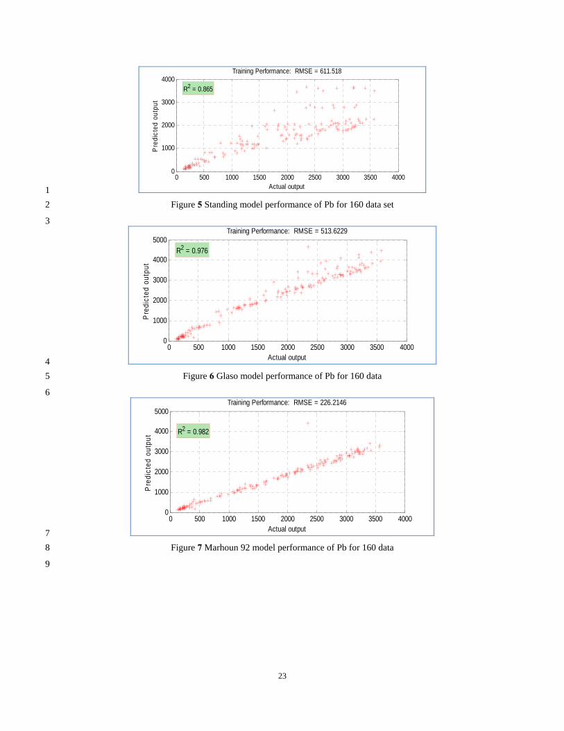
6 Figures 4-15 illustrate six scatter plots of the predicted results versus the experimental data for both Pb and Bob 7

values using the same three distinct data sets. These cross plots indicates the degree of agreement between the 8

experimental and the predicted values based on the high quality performance of the FunNet modeling scheme. The 9

reader can compare theses patterns with the corresponding ones of the published neural networks modeling and 10

common empirical correlations in Al-Marhoun6, Al-Marhoun48, Osman and Abdel-Aal49, and Osman et al.38. Finally, 11

we conclude that developed FunNet modeling scheme has better and reliable performance compared to the most 12

published modeling schemes and empirical correlations. 13

The bottom line is that, the developed FunNet modeling scheme outperforms both the standard feedforward neural 14

networks and the most common published empirical correlations in predicting both Pb and Bob using the four input 15

variables: solution gas-oil ratio, reservoir temperature, oil gravity, and gas relative density. 16

17

18 Figure 4 Pb Performance of 160 data set 19

20

23

0 500 1000 1500 2000 2500 3000 3500 40000

1000

2000

3000

4000

Pre

dict

ed o

utpu

t

Training Performance: RMSE = 611.518

Actual output

R2 = 0.865

1 Figure 5 Standing model performance of Pb for 160 data set 2

3

0 500 1000 1500 2000 2500 3000 3500 40000

1000

2000

3000

4000

5000

Pre

dict

ed o

utpu

t

Training Performance: RMSE = 513.6229

Actual output

R2 = 0.976

4 Figure 6 Glaso model performance of Pb for 160 data 5

6

0 500 1000 1500 2000 2500 3000 3500 40000

1000

2000

3000

4000

5000

Pre

dict

ed o

utpu

t

Training Performance: RMSE = 226.2146

Actual output

R2 = 0.982

7 Figure 7 Marhoun 92 model performance of Pb for 160 data 8

9

24

1 1.2 1.4 1.6 1.8 21

1.5

2

Pre

dict

ed o

utpu

t

Training Performance: RMSE = 0.014595

Actual output

R2 = 0.997

1 1.2 1.4 1.6 1.8 21

1.5

2P

redi

cted

out

put

Testing Performance: RMSE = 0.011748

Actual Output

R2 = 0.999

1 Figure 8 ANN model performance of Pb for 160 data set 2

3

0 500 1000 1500 2000 2500 3000 3500 40000

1000

2000

3000

4000

Pre

dict

ed o

utpu

t

Training Performance: RMSE = 67.7134 and MDL = 502.7821

Actual output

R2 = 0.998

0 500 1000 1500 2000 2500 3000 35000

1000

2000

3000

4000

Pre

dict

ed o

utpu

t

Testing Performance: RMSE = 47.7293 and MDL = 502.7821

Actual Output

R2 = 0.999

4 Figure 9 FunNet model performance of Pb for 160 data 5

6

7 Table 4 Pb performance of 160 data set 8

Er Ea Emin Emax RMSE SD R Standing 12.811 24.684 0.62334 59.038 611.52 25.159 0.86537

Glaso -18.887 26.551 0.28067 98.78 513.62 25.171 0.97569

25

Marhoun 5.1023 8.9416 0.13115 87.989 226.21 12.839 0.98234 NN training -1.3049 5.2929 0.009235 41.471 56.712 9.6324 0.99854 NN testing -3.1499 7.3483 0.22508 69.015 59.172 14.871 0.9988

FunNet training -0.34191 5.3787 0.039086 45.405 67.713 9.2256 0.99802 FunNet testing -0.53716 5.6194 0.086737 46.107 47.729 10.097 0.99914

1

Table 5 Bo performance of 160 data set 2

Er Ea Emin Emax RMSE SD R Standing -2.628 2.7202 0.016741 13.292 0.057954 2.5823 0.9953 Glaso -0.45136 2.0084 0.03218 11.075 0.041129 2.673 0.99352 Marhoun -0.55292 0.9821 0.008597 6.5123 0.020783 1.2842 0.99586 NN training 0.12729 0.84748 0.036196 4.6519 0.014595 1.109 0.99748 NN testing -0.0709 0.66818 0.085465 2.3676 0.011748 0.89835 0.99897 FunNet training -0.00932 0.66562 0.001801 3.9941 0.011498 0.9197 0.99839 FunNet testing 0.20413 0.4922 0.010289 1.3852 0.007869 0.58667 0.99943

3

0.5 1 1.5 2 2.50.8

0.85

0.9

0.95

1

1.05

Absolute Percent Relative Error (EA)

Cor

rela

tion

Coe

ffici

ent (

Rho

)

Standing (1947)Glaso (1980)Al-Marhoun (1992)ANN TrANN TsFunNet TrFunNet Ts

4 Figure 10 Bo performance of 160 data 5

6

26

1 1.1 1.2 1.3 1.4 1.5 1.6 1.7 1.8 1.9 21

1.5

2

2.5

Pre

dict

ed o

utpu

t

Training Performance: RMSE = 0.057954

Actual output

R2 = 0.995

1 Figure 11 Standing model performance of Bo for 160 data 2

1 1.1 1.2 1.3 1.4 1.5 1.6 1.7 1.8 1.9 21

1.5

2

2.5

Pre

dict

ed o

utpu

t

Training Performance: RMSE = 0.041129

Actual output

R2 = 0.994

3

Figure 12 Glaso model performance of Bo for 160 data 4

5

1 1.1 1.2 1.3 1.4 1.5 1.6 1.7 1.8 1.9 21

1.5

2

2.5

Pre

dict

ed o

utpu

t

Training Performance: RMSE = 0.020783

Actual output

R2 = 0.996

6 Figure 13 Marhoun model performance of Bo for 160 data 7

27

1 1.1 1.2 1.3 1.4 1.5 1.6 1.7 1.8 1.9 21

1.2

1.4

1.6

1.8

2

Pre

dict

ed o

utpu

t

Training Performance: RMSE = 0.014595

Actual output

R2 = 0.997

1 1.1 1.2 1.3 1.4 1.5 1.6 1.7 1.8 1.9 21

1.2

1.4

1.6

1.8

2

Pre

dict

ed o

utpu

t

Testing Performance: RMSE = 0.011748

Actual Output

R2 = 0.999

1 Figure 14 ANN model performance of Bo for 160 data 2

1 1.2 1.4 1.6 1.8 21

1.5

2

2.5

Pre

dict

ed o

utpu

t

Training Performance: RMSE = 0.011498 and MDL = -481.2753

Actual output

R2 = 0.998

1 1.2 1.4 1.6 1.8 21

1.5

2

Pre

dict

ed o

utpu

t

Testing Performance: RMSE = 0.0078693 and MDL = -481.2753

Actual Output

R2 = 0.999

3 Figure 15 FunNet model performance of Bo for 160 data 4

5.0 conclusion and Recommendation 5

In this study, three distinct published data sets were used in investigating the capability of the FunNets modeling 6

scheme as a new framework for predicting the PVT properties of oil crude systems. Based on the obtained results 7

and comparative studies, the conclusions and recommendations can be drawn as follows: 8

A new computational intelligence modeling scheme based on the FunNets scheme to predict both bubble point 9

pressure and oil formation volume factor using the four input variables: solution gas-oil ratio, reservoir temperature, 10

28

oil gravity, and gas relative density. As it is shown in the petroleum engineering communities, these two predicted 1

properties were considered the most important PVT properties of oil crude systems. 2

3 - The developed FunNets modeling scheme outperforms both the standard feedforward neural networks and the 4

most common published empirical correlations. Thus, the developed FunNets modeling scheme has better, 5

efficient, and reliable performance compared to the most published correlations. 6

- The developed FunNets modeling scheme shown a high accuracy in predicting the Bob values with a stable 7

performance, and achieved the lowest absolute percent relative error, lowest minimum error, lowest maximum 8

error, lowest root mean square error, and the highest correlation coefficient among other correlations for the 9

used three distinct data sets. 10

11 The functional networks modeling scheme is flexible, reliable, and shows bright future in implementing it for the oil 12

and gas industry, especially permeability and porosity prediction, history matching, predicting the rock mechanics 13

properties, and seismic litho-faceis classification. 14

NOMENCLATURE 15

Bob = OFVF at the bubble- point pressure, RB/STB 16

Rs = on solution gas oil ratio, SCF/STB 17

T = reservoir temperature, degrees Fahrenheit 18

γo = oil relative density (water=1.0) 19

γg = gas relative density (air=1.0) 20

Er = average percent relative error 21

Ei = percent relative error 22

Ea = average absolute percent relative error 23

Emax = Maximum absolute percent relative error 24

Emin = Minimum absolute percent relative error 25

RMS = Root Mean Square error 26

29

Acknowledgement 1

The authors wish to thank King Fahd University of Petroleum and Minerals and Mansoura University for the 2

facilities utilized to perform the present work and for their support. 3

References 4

1. Standing M.B.: “A Pressure-Volume-Temperature Correlation for Mixtures of California Oils and Gases,” 5

Drill&Prod. Pract., API (1947), pp 275-87. 6

2. Katz, D. L.: “Prediction of Shrinkage of Crude Oils,” Drill&Prod. Pract., API (1942), pp 137-147. 7

3. Standing, M. B.: Volumetric and Phase Behavior of Oil Field Hydrocarbon System. Millet Print Inc., 8

Dallas, TX (1977) 124. 9

4. Vazuquez, M. and Beggs, H.D.: “Correlation for Fluid Physical Property Prediction,” JPT (June 1980) 10

968. 11

5. Glaso, O. “Generalized Pressure-Volume Temperature Correlations,” JPT (May 1980), 785. 12

6. Al-Marhoun, M., “PVT Correlations for Middle East Crude Oils,” Journal of Petroleum Technology, pp 13

650-666, 1988. 14

7. Abdul-Majeed, G.H.A. and Salman, N.H.: “An Empirical Correlation for FVF Prediction,” JCPT, (July-15

August 1988) 118. 16

8. Labedi, R.: “Use of Production Data to Estimate Volume Factor Density and Compressibility of Reservoir 17

Fluids.” J. Pet. Sci. & Eng., 4(1990) 357. 18

9. Dokla, M. and Osman, M.: “Correlation of PVT Properties for UAE Crudes,” SPEFE (March 1992) 41. 19

10. Al-Yousef H. Y., Al-Marhoun, M. A.: “Discussion of Correlation of PVT Properties for UAE Crudes,” 20

SPEFE (March 1993) 80. 21

11. Dokla, M. and Osman, M.: “Authors’ Reply to Discussion of Correlation of PVT Properties for UAE 22

Crudes,” SPEFE (March 1993) 82. 23

12. Al-Marhoun, M. A.: “New Correlation for formation Volume Factor of oil and gas Mixtures,” JCPT 24

(March 1992) 22. 25

30

13. Macary, S. M. & El-Batanoney, M. H.: “Derivation of PVT Correlations for the Gulf of Suez Crude Oils,” 1

Paper presented at the EGPC 11th Petroleum Exploration & Production Conference, Cairo, Egypt (1992). 2

14. Saleh, A. M., Maggoub, I. S. and Asaad, Y.: “Evaluation of Empirically Derived PVT Properties for 3

Egyptian Oils,” paper SPE 15721 , presented at the 1987 Middle East Oil Show & Conference, Bahrain, 4

March 7-10. 5

15. Omar, M.I. and Todd, A.C.: “Development of New Modified Black oil Correlation for Malaysian Crudes,” 6

paper SPE 25338 presented at the 1993 SPE Asia Pacific Asia Pacific Oil & Gas Conference and 7

Exhibition, Singapore, Feb. 8-10. 8

16. Petrosky, J. and Farshad, F.: “Pressure Volume Temperature Correlation for the Gulf of Mexico.” paper 9

SPE 26644 presented at the 1993 SPE Annual Technical Conference and Exhibition, Houston, TX, Oct 3-10

6. 11

17. Kartoatmodjo, T. and Schmidt, Z.: “Large data bank improves crude physical property correlations,” Oil 12

and Gas Journal (July 4, 1994) 51. 13

18. Almehaideb, R.A.: “Improved PVT Correlations For UAE Crude Oils,” paper SPE 37691 presented at the 14

1997 SPE Middle East Oil Show and Conference, Bahrain, March 15–18. 15

19. Sutton, R. P. and Farshad, F.: ” Evaluation of Empirically Derived PVT Properties for Gulf of Mexico 16

Crude Oils” SPRE (Feb. 1990) 79. 17

20. Sutton, Roberts P. and Farshad, F.: ”Supplement to SPE 1372, Evaluation of Empirically Derived PVT 18

Properties for Gulf of Mexico Crude Oils” SPE 20277, Available from SPE book Order Dep., Richardson, 19

TX. 20

21. McCain, W. D.: “ Reservoir fluid property correlations-State of the Art,” SPERE, (May 1991) 266. 21

22. Ghetto, G. De, Paone, F. and Villa, M.: “Reliability Analysis on PVT correlation,” paper SPE 28904 22

presented at the 1994 SPE European Petroleum Conference, London, UK, October 25-27. 23

23. Elsharkawy, A. M. Elgibaly, A. and Alikhan, A. A.: “Assessment of the PVT Correlations for Predicting 24

the Properties of the Kuwaiti Crude Oils,” paper presented at the 6th Abu Dhabi International Petroleum 25

Exhibition & Conference, Oct. 16-19, 1994. 26

31

24. Mahmood, M. M. and Al-Marhoun, M. A.: “Evaluation of empirically derived PVT properties for 1

Pakistani crude oils,” J. Pet. Sci. & Engg. 16 (1996) 275. 2

25. Hanafy, H.H., Macary, S.A., Elnady, Y. M., Bayomi, A.A. and El-Batanoney, M.H.: “ Empirical PVT 3

Correlation Applied to Egyptian Crude Oils Exemplify Significance of Using Regional Correlations,” 4

paper SPE 37295 presented at the SPE Oilfield Chemistry International Symposium, Houston, Feb. 18–21, 5

1997. 6

26. Al-Fattah, S. M. and Al-Marhoun, M. A.: “Evaluation of empirical correlation for bubble point oil 7

formation volume factor,” J. Pet. Sci. & Engg. 11(1994) 341. 8

27. Al-Shammasi, A. A.,: “Bubble Point Pressure and Oil Formation Volume Factor Correlations,” paper SPE 9

53185 presented at the 1997 SPE Middle East Oil Show and Conference, Bahrain, March 15–18. 10

28. Kumoluyi, A.O. and Daltaban, T.S.: “High-Order Neural Networks in Petroleum Engineering,” paper SPE 11

27905 presented at the 1994 SPE Western Regional Meeting, Longbeach, California, USA, March 23-25. 12

29. Ali, J. K.: “Neural Networks: A New Tool for the Petroleum Industry,” paper SPE 27561 presented at the 13

1994 European Petroleum Computer Conference, Aberdeen, U.K., March 15-17. 14

30. Mohaghegh, S. and Ameri, S.,:" A Artificial Neural Network As A Valuable Tool For Petroleum 15

Engineers," SPE 29220, unsolicited paper for Society of Petroleum Engineers, 1994. 16

31. Mohaghegh, S.:" Neural Networks: What it Can do for Petroleum Engineers," JPT, (Jan. 1995) 42. 17

32. Mohaghegh, S.:" Virtual Intelligence Applications in Petroleum Engineering: Part 1 - Artificial Neural 18

Networks,” JPT (September 2000). 19

33. Gharbi, R.B. and Elsharkawy, A.M.: “Neural-Network Model for Estimating the PVT Properties of Middle 20

East Crude Oils,” paper SPE 37695 presented at the 1997 SPE Middle East Oil Show and Conference, 21

Bahrain, March 15–18. 22

34. Gharbi, R.B. and Elsharkawy, A.M.: “Universal Neural-Network Model for Estimating the PVT Properties 23

of Crude Oils,” paper SPE 38099 presented at the 1997 SPE Asia Pacific Oil & Gas Conference, Kuala 24

Lumpur, Malaysia, April 14-16. 25

35. Elsharkawy, A.M.: “Modeling the Properties of Crude Oil and Gas Systems Using RBF Network,” paper 26

SPE 49961 presented at the 1998 SPE Asia Pacific Oil & Gas Conference, Perth, Australia, October 12-14. 27

32

36. Varotsis N., Gaganis V., Nighswander J., and Guieze P.,: “A Novel Non-Iterative Method for the 1

Prediction of the PVT Behavior of Reservoir Fluids,” paper SPE 56745 presented at the 1999 SPE Annual 2

Technical Conference and Exhibition, Houston, Texas, October 3–6. 3

37. Farshad, F.F, Leblance, J.L, Garber, J.D. and Osorio, J.G.: “Empirical Correlation for Colombian Crude 4

Oils,” paper SEP 24538, Unsolicited (1992), Available from SPE book Order Dep., Richardson, TX. 5

38. Osman, E. A., Abdel-Wahhab, O. A., and Al-Marhoun, M. A., “Prediction of Oil Properties Using Neural 6

Networks,” Paper SPE 68233, 2001. 7

39. Hinton G. E., “Connectionist learning procedures”. Artificial Intel., 40:185–234, 1989. 8

40. White H., “Learning in artificial neural networks: A statistical perspective”. Neural Comput., 1:425–464, 9

1989. 10

41. Hussam M. Goda, Eissa M. El-M Shokir, Khaled A. Fattah, and Mohamed H. Sayyouh "Prediction of the 11

PVT Data using Neural Network Computing Theory". The 27th Annual SPE International Technical 12

Conference and Exhibition in Abuja, Nigeria, August 4-6, 2003: SPE85650. 13

42. Ali, J. K., “Neural Networks: A New Tool for the Petroleum Industry,” Paper SPE 27561, 1994. 14

43. Duda R. O., Hart P. E., and Stock D. G., “Pattern Classification, Second Edition, John Wiley and Sons, 15

New York, 2001. 16

44. Danesh, A., “PVT and Phase Behavior of Petroleum Reservoir Fluid,” Elsevier Publishing Company, 17

1998. 18

45. Smith, C., Tracy, G., and Farrar, R., “Applied Reservoir Engineering, Volume 1,” Oil & Gas Consultants 19

International, Inc., 1992. 20

46. Al-Shammasi, A. A.: “Bubble Point Pressure and Oil Formation Volume Factor Correlations,” SPE Middle 21

East Oil Show, Bahrain, 20–23 February 1999. SPE53185. 22

47. Al-Shammasi, A. A.: “A Review of Bubble point Pressure and Oil Formation Volume Factor 23

Correlations,” SPE Reservoir Evaluation & Engineering (April 2001) 146-160. This paper (SPE 71302) 24

was revised for publication from paper SPE 53185. 25

33

48. Al-Marhoun, M.A., and Osman, E. A., “Using Artificial Neural Networks to Develop New PVT 1

Correlations for Saudi Crude Oils,” Paper SPE 78592, presented at the 10th Abu Dhabi International 2

Petroleum Exhibition and Conference (ADIPEC), Abu Dhabi, UAE, October 8-11, 2002. 3

49. Osman E. A. and Abdel-Aal, "Abductive Netwoks: A New Modeling Tool for the Oil and Gas Industry". 4

SPE 77882 Asia Pacific Oil and Gas Conference and Exhibition Melbourne, Australia, 8–10 October 2002. 5

50. Osman E., Al-Marhoun M., “Artificial Neural Networks Models for Predicting PVT Properties of Oil Field 6

Brines", paper SPE 93765, 14th SPE Middle East Oil & Gas Show and Conference in Bahrain, March 7

2005. 8

51. McCain W. D. Jr., R. Soto B., Valko, P.P., and Blasingame, T. A. “Correlation Of Bubble point Pressures 9

For Reservoir Oils - A Comparative Study,” paper SPE 51086 presented at the 1998 SPE Eastern Regional 10

Conference and Exhibition held in Pittsburgh, PA, 9–11 November. 11

52. Castillo E., Cobo A., Gutiérrez J. M. and Pruneda E., (1998), Introduction to Functional Networks with 12

Applications, A Neural Based Paradigm, Kluwer Academic Publishers: New York. 13

53. E. El-Sebakhy, “Constrained Estimation of Functional Networks for Statistical Pattern Recognition 14

Problems”, Journal of AI and Patt. Rec. In Press, 2007. 15

54. E. Castello, Functional networks. Neural Proc. Lett. 7 (1998), pp. 151¯159. 16

55. S. Rajasekaran, V. Shalu Mohan, and O. Khamis, (2004), "The optimisation of space structures using 17

evolution strategies with functional networks", Engineering with Computers (2004) 20: 75–87. Springer-18

Verlag London. 19

56. M. Bruen and J.C.I. Dooge, An efficient and robust method for estimating unit hydrograph ordinates, J 20

Hydrol 70 (1984), pp. 1–24. 21

57. E. Castillo, J. M. GutiCrrez, (1998), “Nonlinear time series modeling and prediction using functional 22

networks. Extracting information masked by chaos”. Physics Letters A (244) 71-84. 23

58. El-Sebakhy A. E., Functional Networks Training Algorithm for Statistical Pattern Recognition; IEEE 24

Symposium on Computers and Communications, ISCC 2004. Ninth International Symposium on Volume, 25

vol. 1, pp. 92 –97, 28 June–1 July, 2004. 26

34

59. El-Sebakhy A. E., Hadi S. A., and Faisal A. K., Iterative Least Squares Functional Networks Classifier; 1

IEEE Transactions Neural Networks, vol. 18, no. 3, pp. 844 –850, March 2007. 2

60. El-Sebakhy E., Faisal K., El-Bassuny T., Azzedin F., and Al-Suhaim A., (2006), “Evaluation of Breast 3

Cancer Tumor Classification with Unconstrained Functional Networks Classifier”; the 4th ACS/IEEE 4

International Conf. on Computer Systems and Applications. 281-287. 5

61. El-Sebakhy A. E., “Relative Solvent Accessibility of Residues in Proteins Using Unconstrained Functional 6

Networks”, International Journal of Bioinformatics (2007). (In press). 7

62. El-Sebakhy A. E. and Albokhitan Y. S., “Forecasting PVT Properties of Crude Oil Systems based on 8

Support Vector Machines Modeling Scheme”. International journal of Mathematics and Computers In 9

Simulation, (2007). (In press). 10

63. Li C, Liao X, Wu Z, Yu J. Complex functional networks. Math Comput Simul 2001;57:355–65. 11

64. Castillo E., Functional networks. Neural Process. Lett., 7(3):151–159, 1998. 12

65. Castillo E, Cobo A, Gutierrez JM, Pruneda E., Functional networks with applications-a neural-based 13

paradigm. Boston/ Dordrecht/London: Kluwer Academic Publishers; New York, 1998. 14

66. Castillo E, Cobo A, Gutierrez JM, and Hadi A. S., A general framework for functional networks. 15

Networks, 35:70–82, 1999. 16

67. Castillo E. and Gutierrez JM,, A comparison of functional networks and neural networks. In Proceedings 17

of the IASTED International Conference on Artificial Intelligence and Soft Computing, pages 439–442, 18

IASTED ACTA press 1998. 19

68. Castillo E, Cobo A, Gutierrez JM, Pruneda E.,, Working with differential, functional and di erence 20

equations using functional networks. Applied Mathematical Modelling 23 (1999) 89 – 107. 21

69. Castillo E, Cobo A, Gutierrez JM, Nonlinear time series modeling and prediction using functional 22

networks. Extracting information masked by chaos. Physics Letters A 244 (1998) 71-84. 23

70. Castillo, E., Hadi, A., and Lacruz, B. (2001), "Optimal Transformations in Multiple Linear Regression 24

Using Functional Networks," Proceedings of the International Work-Conference on Artificial and natural 25

Neural Networks. IWANN 2001, in Lecture Notes in Computer Science 2084, Part I, 316–324. 26

35

71. Castillo, E., Gutiérrez, J. M., Hadi, A. S., and Lacruz, B. (2001), "Some Applications of Functional 1

Networks in Statistics and Engineering," Technometrics, 43, 10–24. 2

72. Pruneda, B. Lacruz, and C. Solares, A First Approach to Solve Classification Problems Based on 3

Functional Networks. ICANN 2005, LNCS 3697, pp. 313–318. Springer-Verlag Berlin Heidelberg 2005. 4

73. Solares C., Vieira E. W., and Minguez R., Functional Networks and the Lagrange Polynomial 5

Interpolation. E. Corchado et al. (Eds.): IDEAL 2006, LNCS 4224, pp. 394–401, 2006. Springer-Verlag 6

Berlin Heidelberg 2006. 7

74. Rajasekaran S., Mohan V. S., and Khamis O., The optimization of space structures using evolution 8

strategies with functional networks. Engineering with Computers (2004) 20: 75–87. 9

75. [28] Bruen M. and Yang J., Functional networks in real-time flood forecasting- a novel application. 10

Advances in Water Resources 28 (2005) 899–909 11

12

13

1 14

15

36

Appendices 1

Table 6 Performance of Pb for 283 data set 2   Er  Ea  Emin  Emax  RMSE  SD  R 

Standing  10.198  19.81  0.25511  93.672  425.19  22.252  0.89739 Glaso  ‐17.262  21.418  1.4363  70.407  377.72  18.349  0.98371 

Marhoun  8.8175  10.56  0.053296  57.593  193.63  9.9281  0.99054 NN training  ‐1.015  4.4734  0.015138  129.62  52.162  12.183  0.99804 NN testing  ‐3.3969  5.9478  0.024248  98.647  58.741  13.662  0.99843 

FunNet training  ‐0.12266  5.2877  0.013004  49.056  62.256  8.3431  0.99717 FunNet testing  2.8209  4.4175  0.045593  33.382  55.77  6.3978  0.99852 

 3

5 10 15 200.7

0.75

0.8

0.85

0.9

0.95

1

1.05

Absolute Percent Relative Error (EA)

Cor

rela

tion

Coe

ffici

ent (

Rho

)

Standing (1947)Glaso (1980)Al-Marhoun (1992)ANN TrANN TsFunNet TrFunNet Ts

 4 Figure 16  Pb Performance for 283 data set 5

 6  7

0 500 1000 1500 2000 2500 3000 35000

1000

2000

3000

4000

Pre

dict

ed o

utpu

t

Training Performance: RMSE = 425.1929

Actual output

R2 = 0.897

 8 Figure 17  Standing Pb Performance for 283 data set 9

37

 1

0 500 1000 1500 2000 2500 3000 35000

1000

2000

3000

4000

5000

Pre

dict

ed o

utpu

t

Training Performance: RMSE = 377.7177

Actual output

R2 = 0.984

 2 Figure 18 Glaso Pb Performance for 283 data set 3

 4

0 500 1000 1500 2000 2500 3000 35000

1000

2000

3000

4000

Pre

dict

ed o

utpu

t

Training Performance: RMSE = 193.6304

Actual output

R2 = 0.991

 5 Figure 19 Marhoun Pb Performance for 283 data set 6

 7

0 500 1000 1500 2000 2500 3000 35000

1000

2000

3000

4000

Pre

dict

ed o

utpu

t

Training Performance: RMSE = 52.1623

Actual output

R2 = 0.998

0 500 1000 1500 2000 2500 3000 35000

1000

2000

3000

4000

Pre

dict

ed o

utpu

t

Testing Performance: RMSE = 58.7409

Actual Output

R2 = 0.998

 8 Figure 20 ANN  Pb Performance for 283 data set 9

38

 1  2

0 500 1000 1500 2000 2500 3000 35000

1000

2000

3000

4000

Pre

dict

ed o

utpu

t

Training Performance: RMSE = 62.2558 and MDL = 853.879

Actual output

R2 = 0.997

0 500 1000 1500 2000 2500 3000 35000

1000

2000

3000

4000

Pre

dict

ed o

utpu

t

Testing Performance: RMSE = 55.77 and MDL = 853.879

Actual Output

R2 = 0.999

 3 Figure 21 FunNet Pb Performance for 283 data set 4

 5

2 Table 7 Performance of Bo for 283 data set 6

  Er  Ea  Emin  Emax  RMSE  SD  R Standing  ‐1.9738  2.1334  0.013382  13.337  0.044046  2.2257  0.99465 Glaso  0.2157  1.7939  0.002994  11.539  0.032632  2.3297  0.99197 Marhoun  ‐0.74564  1.0037  0.001112  5.0515  0.019915  1.1431  0.99722 NN training  0.35333  0.64064  0.002366  3.1729  0.01134  0.77523  0.99765 NN testing  0.26255  0.65798  0.002105  2.8004  0.010851  0.80728  0.99843 FunNet training  ‐0.00472  0.53251  0.006154  2.8419  0.008861  0.68708  0.99839 

FunNet testing 0.00654

4  0.34755  0.002623  2.6395  0.00624  0.50494  0.99926 

 7

Table 8 Performance of Pb for 782 data set 8

  Er  Ea  Emin  Emax  RMSE  SD  R Standing  67.602  67.73  0.16209  102.08  1609.3  13.696  0.86661 Glaso  ‐1.6162  18.523  0.10563  138.96  473.3  25.27  0.94471 

Marhoun  8.0076  20.011  0.025427  109.12  593.81  25.015  0.90583 NN training  ‐6.2973  15.098  0.023293  157.58  326.97  21.73  0.96786 NN testing  ‐10.4  16.345  0.13776  117.43  282.54  20.821  0.97887 

FunNet training  ‐5.2249  15.751  0.084898  173.29  344.69  24.745  0.9618 FunNet testing  ‐2.1471  13.361  0.068983  176.07  303.75  20.792  0.97558 

 9

39

 1 Figure 22 Performance of Bo for 283 data set 2

 3

1 1.1 1.2 1.3 1.4 1.5 1.6 1.7 1.8 1.91

1.5

2

2.5

Pre

dict

ed o

utpu

t

Training Performance: RMSE = 0.044046

Actual output

R2 = 0.995

 4 Figure 23  Standing Bo Performance for 283 data set 5

 6

1 1.1 1.2 1.3 1.4 1.5 1.6 1.7 1.8 1.91

1.2

1.4

1.6

1.8

2

Pre

dict

ed o

utpu

t

Training Performance: RMSE = 0.032632

Actual output

R2 = 0.992

 7 Figure 24 Glaso Bo Performance for 283 data set 8

 9

40

1 1.1 1.2 1.3 1.4 1.5 1.6 1.7 1.8 1.91

1.2

1.4

1.6

1.8

2

Pre

dict

ed o

utpu

t

Training Performance: RMSE = 0.019915

Actual output

R2 = 0.997

 1 Figure 25 Marhoun Bo Performance for 283 data set 2

 3

1 1.1 1.2 1.3 1.4 1.5 1.6 1.7 1.8 1.91

1.5

2

Pre

dict

ed o

utpu

t

Training Performance: RMSE = 0.01134

Actual output

R2 = 0.998

1 1.1 1.2 1.3 1.4 1.5 1.6 1.7 1.8 1.91

1.5

2

Pre

dict

ed o

utpu

t

Testing Performance: RMSE = 0.010851

Actual Output

R2 = 0.998

 4 Figure 26 ANN Bo Performance for 283 data set 5

 6  7

0 500 1000 1500 2000 2500 3000 35000

1000

2000

3000

4000

Pre

dict

ed o

utpu

t

Training Performance: RMSE = 62.2558 and MDL = 853.879

Actual output

R2 = 0.997

0 500 1000 1500 2000 2500 3000 35000

1000

2000

3000

4000

Pre

dict

ed o

utpu

t

Testing Performance: RMSE = 55.77 and MDL = 853.879

Actual Output

R2 = 0.999

 8 Figure 27 FunNet Bo Performance for 283 data set 9

41

 1

15 20 25 30 35 40 45 50 55 60 65

0.7

0.75

0.8

0.85

0.9

0.95

1

1.05

Absolute Percent Relative Error (EA)

Cor

rela

tion

Coe

ffici

ent (

Rho

)

Standing (1947)Glaso (1980)Al-Marhoun (1992)ANN TrANN TsFunNet TrFunNet Ts

 2 Figure 28 Performance of Pb for 782 data set 3

 4

0 1000 2000 3000 4000 5000 6000 7000 8000-1000

0

1000

2000

3000

4000

Pre

dict

ed o

utpu

t

Training Performance: RMSE = 1609.2527

Actual output

R2 = 0.867

 5 Figure 29 Standing Pb Performance for 782 data set 6

 7

0 1000 2000 3000 4000 5000 6000 7000 80000

2000

4000

6000

8000

Pre

dict

ed o

utpu

t

Training Performance: RMSE = 473.299

Actual output

R2 = 0.945

 8 Figure 30 Glaso Pb Performance for 782 data set 9

42

0 1000 2000 3000 4000 5000 6000 7000 80000

2000

4000

6000

8000

10000

Pre

dict

ed o

utpu

t

Training Performance: RMSE = 593.8129

Actual output

R2 = 0.906

 1 Figure 31 Marhoun Performance for 782 data set 2

 3

0 1000 2000 3000 4000 5000 6000 70000

2000

4000

6000

8000

Pre

dict

ed o

utpu

t

Training Performance: RMSE = 326.9711

Actual output

R2 = 0.968

0 1000 2000 3000 4000 5000 6000 7000 80000

2000

4000

6000

8000

Pre

dict

ed o

utpu

t

Testing Performance: RMSE = 282.541

Actual Output

R2 = 0.979

 4 Figure 32 ANN Pb Performance for 782 data set 5

 6

 7 Figure 33 FunNet Pb Performance for 782 data set 8

43

Table 9 Performance of Bo for 782 data set 1

  Er  Ea  Emin  Emax  RMSE  SD  R Standing  ‐1.6353  3.1083  0.010503  89.786  0.099927  5.7655  0.95621 Glaso  1.0911  3.2591  0.011654  65.773  0.083353  5.2274  0.96009 

Marhoun  ‐0.78385  2.5738  0.009682  60.354  0.082717  5.0028  0.95986 NN training  ‐0.18716  2.2458  0.009277  35.814  0.066396  4.0402  0.97106 

NN testing 0.01351

6  1.9103  0.002308  10.128  0.04241  2.5873  0.98763 FunNet training  ‐0.13669  2.0913  0.002445  38.728  0.056962  3.8214  0.97848 FunNet testing  ‐0.22852  1.7134  0.001953  8.1564  0.033451  2.3508  0.99272 

 2  3

1.8 2 2.2 2.4 2.6 2.8 3 3.2

0.8

0.85

0.9

0.95

1

1.05

Absolute Percent Relative Error (EA)

Cor

rela

tion

Coe

ffici

ent (

Rho

)

Standing (1947)Glaso (1980)Al-Marhoun (1992)ANN TrANN TsFunNet TrFunNet Ts

 4 Figure 34 Performance of Bo for 782 data set 5

 6

1 1.2 1.4 1.6 1.8 2 2.2 2.4 2.6 2.8 31

2

3

4

Pre

dict

ed o

utpu

t

Training Performance: RMSE = 0.099927

Actual output

R2 = 0.956

 7 Figure 35 Standing Bo Performance for 782 data set 8

 9

44

1 1.2 1.4 1.6 1.8 2 2.2 2.4 2.6 2.8 31

1.5

2

2.5

3

3.5

Pre

dict

ed o

utpu

t

Training Performance: RMSE = 0.083353

Actual output

R2 = 0.960

 1 Figure 36 Glaso Bo Performance for 782 data set 2

 3

1 1.2 1.4 1.6 1.8 2 2.2 2.4 2.6 2.8 31

1.5

2

2.5

3

3.5

Pre

dict

ed o

utpu

t

Training Performance: RMSE = 0.082717

Actual output

R2 = 0.960

 4 Figure 37 Marhoun Bo Performance for 782 data set 5

 6

1 1.5 2 2.5 31

1.5

2

2.5

3

Pre

dict

ed o

utpu

t

Training Performance: RMSE = 0.066396

Actual output

R2 = 0.971

1 1.5 2 2.5 31

1.5

2

2.5

3

Pre

dict

ed o

utpu

t

Testing Performance: RMSE = 0.04241

Actual Output

R2 = 0.988

 7 Figure 38  ANN Bo Performance for 782 data set 8

 9

45

1 1.5 2 2.5 31

2

3

4

Pre

dict

ed o

utpu

t

Training Performance: RMSE = 0.056962 and MDL = -1544.9958

Actual output

R2 = 0.978

1 1.5 2 2.5 31

1.5

2

2.5

3

Pre

dict

ed o

utpu

t

Testing Performance: RMSE = 0.033451 and MDL = -1544.9958

Actual Output

R2 = 0.993

 1 Figure 39 FunNet Bo Performance for 782 data set 2