Embed Size (px)
Citation preview

Estimating LGD with stochastic collateral
Robert Frontczak†‡ Stefan Rostek§
First Version: January, 2013.
This Version: January, 2014.
Abstract
This article addresses to the appropriate modeling of loss given default
(LGD) for the retail business sector. We assume small or mid-size loans that
are assigned in a standardized way and collateralized by residential or com-
mercial property. The focus on this specific type of loans entails two major
advantages: Firstly, reduction of complexity is followed by easier-to-grasp
methodology and increased handiness of results when comparing with other
recent approaches in the field. Secondly, the focussing allows to take into
account the characteristic properties of the housing market and its under-
lying uncertainty and so choose a tailor-made modeling for the collateral.
The choice of an exponential Ornstein-Uhlenbeck diffusion as the stochastic
process of the collateral combines the desirable features with the charm of
analytical solvability which seems to be of advantage as regards to accep-
tance among practitioners. Further key improvements of this approach are
the explicit consideration of loan ranking, the disentanglement of the time of
default and the time of liquidation as well as the introduction of liquidation
cost.†Landesbank Baden-Wurttemberg (LBBW), Am Hauptbahnhof 2, 70173 Stuttgart,
Germany. Phone: 0711-12770519, E-mail: [email protected]
Disclaimer: Statements and conclusions made in this article are entirely those of the
author. They do not necessarily reflect the views of LBBW.‡Corresponding author§Universitat Tubingen, Lehrstuhl fur Betriebliche Finanzwirtschaft und Allgemeine
Betriebswirtschaftslehre, Sigwartstr.18, 72076 Tubingen, Deutschland. Phone: 07071-29-
72804, E-mail: [email protected]

1 Introduction and motivation
Loss Given Default (LGD) is one of the key measures when modeling and
managing credit risk. It captures the percental loss the bank faces in case of a
defaulting obligor. Since 2006, the Basle Committee on Banking Supervision
(BCBS) allows banks to use their own rating approaches for the purpose of
calculating the required equity for credit collateralization – i.e. a so called
Internal Rating Based Approach (IRBA). This concept stipulates the idea of
expected loss as a product of three factors:
E[L] = PD · EAD · LGD.
The first factor PD represents the probability of default (PD), the sec-
ond one EAD denotes the amount of unredeemed outstanding debt at the
moment the obligor defaults, the exposure at default (EAD). The third com-
ponent yet is the loss given default (LGD) as percentage of nonrecoverable
debt related to EAD. Banks using the advanced rating approach are allowed
to estimate these parameters single-handedly by means of internally devel-
oped methods. If one assumes that the EAD component is predictable to a
great extent by means of amortization schedules, the problem reduces to an
accurate estimation of LGD and PD. For the bank, reliable estimates of each
component are important in equal measure: Correctly estimated (and low)
values for LGD and/or PD lead to lower expected loss and therefore to lower
capital requirements and a reduction of risk capital.
Before proceeding it is worth concretizing the concept of expected loss as
introduced in the equation above. Let us consider a portfolio with N debtors.
For each of them i, i = 1, ..., N, let Di be the digital random variable that
indicates whether the very debtor defaults with possible realizations for Di
to be 1 in case of default and 0 if no default occurs, i.e. Di is a digital random
variable or indicator function. Consequently, the random loss Li in absolute
2
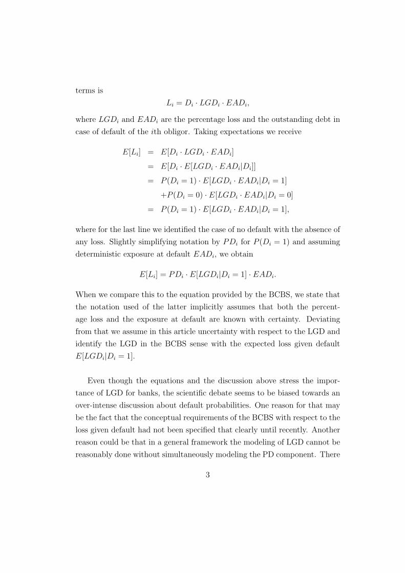
terms is
Li = Di · LGDi · EADi,
where LGDi and EADi are the percentage loss and the outstanding debt in
case of default of the ith obligor. Taking expectations we receive
E[Li] = E[Di · LGDi · EADi]
= E[Di · E[LGDi · EADi|Di]]
= P (Di = 1) · E[LGDi · EADi|Di = 1]
+P (Di = 0) · E[LGDi · EADi|Di = 0]
= P (Di = 1) · E[LGDi · EADi|Di = 1],
where for the last line we identified the case of no default with the absence of
any loss. Slightly simplifying notation by PDi for P (Di = 1) and assuming
deterministic exposure at default EADi, we obtain
E[Li] = PDi · E[LGDi|Di = 1] · EADi.
When we compare this to the equation provided by the BCBS, we state that
the notation used of the latter implicitly assumes that both the percent-
age loss and the exposure at default are known with certainty. Deviating
from that we assume in this article uncertainty with respect to the LGD and
identify the LGD in the BCBS sense with the expected loss given default
E[LGDi|Di = 1].
Even though the equations and the discussion above stress the impor-
tance of LGD for banks, the scientific debate seems to be biased towards an
over-intense discussion about default probabilities. One reason for that may
be the fact that the conceptual requirements of the BCBS with respect to the
loss given default had not been specified that clearly until recently. Another
reason could be that in a general framework the modeling of LGD cannot be
reasonably done without simultaneously modeling the PD component. There
3

are a number of empirical articles that indicate a dependence of PD and LGD:
Altman/Resti/Sironi (2001), Altman/Brady/Resti/Sironi (2005), Caselli/
Gatti/Querci (2008) and Acharya/Bharath/Srinivasan (2007) use regres-
sion based models to show that the economic cycle of an industrial sector
or of the whole economy explains both probabilittes of defaults and histori-
cally realized values of loss given default in a significant way. Hu/Perraudin
(2006) use extreme value theory to prove a direct correlation of PD and LGD
in the US bond market. Bade/Rosch/Scheule (2011) investigate corporate
loans and identify a correlation between the default process (i.e. PD) and
the process of recovery values (i.e. LGD) by means of maximum likelihood
methods.
The existing literature concerning theoretical aspects of LGD, however,
restricts itself to a very general and hardly applicable view of the topic. The
theoretical models usually account for the possible dependence of PD and
LGD in one of the following ways: Frye (2000), Dev/Pykhtin (2002), Hille-
brand (2005), van Damme (2011) und Jacobs (2011) model the recovery
rate as one random variable and the assets of the obligor as a second one and
let both of them be driven by one latent factor. Jokivuolle/Peura (2003) and
Pykhtin (2003) choose correlated stochastic processes for the firm value on
the one hand and the value of the collateral on the other hand. The result-
ing formulas are highly complex but still vague for lack of concretion towards
a realistic and practice-oriented type of collateral. Consequently, trying to
catch ’all by one’, these approaches end up at the lowest common denomina-
tor. Typically, this common denominator is found to be geometric Brownian
motion which then again can neither satisfy researchers nor practitioners.
As we acknowledge the impossibility to capture the heterogeneity of dif-
ferent LGD estimation problems within one general and still powerful model,
we enter the alternative path of specification: In this paper we focus on one
4
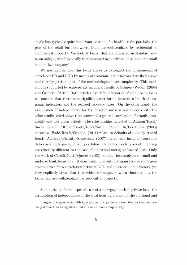
single but typically quite important portion of a bank’s credit portfolio, the
part of the retail business where loans are collateralized by residential or
commercial property. We look at loans, that are conferred in standard way
to an obligor, which typically is represented by a private individual or a small
or mid-size company1.
We now explain how this focus allows us to neglect the phenomenon of
correlated PD and LGD by means of economic latent factors described above
and thereby jettison part of the methodological over-complexity. This mod-
eling is supported by some recent empirical results of Grunert/Weber (2009)
and Grunert (2010): Both articles use default histories of small bank loans
to conclude that there is no significant correlation between a bunch of eco-
nomic indicators and the realized recovery rates. On the other hand, the
assumption of independence for the retail business is not at odds with the
other studies cited above that confirmed a general correlation of default prob-
ability and loss given default: The relationships detected in Altman/Resti/
Sironi (2001), Altman/Brady/Resti/Sironi (2005), Hu/Perraudin (2006)
as well as Bade/Rosch/Scheule (2011) relate to defaults of publicly traded
bonds. Acharya/Bharath/Srinivasan (2007) derive their insights from some
data covering large-cap credit portfolios. Evidently, both types of financing
are crucially different to the case of a classical mortgage-backed loan. Only
the work of Caselli/Gatti/Querci (2008) address their analysis to small and
mid-size bank loans of an Italian bank. The authors again receive some gen-
eral evidence for a correlation between LGD and macroeconomic factors, yet
they explicitly stress that this evidence disappears when choosing only the
loans that are collateralized by residential property.
Summarizing, for the special case of a mortgage-backed private loan, the
assumption of independence of the local housing market on the one hand and
1Large-size engagements with international companies are excluded, as they are cru-
cially different for being structured in a much more complex way.
5

the solvency of the single obligor on the other hand, seems to be feasible or
at least not a major limitation. But what we earn is much more: We obtain
an increased analytic manageability which should also increase acceptance
among practitioners considerably. Meanwhile, the model reduction fans out
a multitude of possibilities for an adequate modeling of the collateralizing
asset. As we focus on residential property, we have a look on mathematical
models of real estate markets (commercial and residential).
With respect to the descriptive and empirical level, there is early work of
Case/Shiller (1989), Case/Shiller (1990) and Hosios/Pesando (1991). All
three emphasize the incompleteness of real estate markets and elaborate the
phenomenon of serial correlation to be a key ingredient of an appropriate
mathematical model. Furthermore, seasonality seems to play an important
role for the studies dealing with local housing prices in Chicago (Case/Shiller)
and Toronto (Hosios/Pesando). Englund/Ioannides (1997) affirm these re-
lationships when investigating international data sets. A number of articles
tries to ascribe these stylized facts to search-theoretic (see Wheaton (1990),
Krainer (2001), Piazzesi/Schneider (2009), Novy-Marx (2009) and Diaz/
Jerez (2013)) and/or behavioristic (see e.g. Hott (2011)) mechanisms.
Despite of these insights the early literature dealing with derivative pric-
ing in the real estate sector are based on the assumption of complete markets
and geometric Brownian motion as stochastic model (see Titman/Torous
(1989), Buttimer/Kau/Slawson (1997) and Bjork/Clapham (2002)). Later
models keep geometric Brownian motion as driving diffusive process but in-
troduce equilibrium models to account for market incompleteness (see Gelt-
ner/Fisher (2007) and Cao/Wei (2010)). Crawford/Fratantoni (2003) sug-
gest ARIMA- and GARCH- models for a realistic mapping of house price
indices. The recent work of Fabozzi/Shiller/Tunaru (2010) again stresses
the need of a mathematical model that incorporates serial correlation and
6

provides new empirical evidence. The model the authors suggest ties in
with the approaches of Lo/Wang (1995) and Jokivuolle (1998) who deal
with other serially correlated assets. Finally, Fabozzi/Shiller/Tunaru (2012)
point out that the property of serial correlation must be regarded as a cen-
tral requirement when modeling any kind of real estate. The process these
authors use and which also Perello/Sircar/Masoliver (2008) use in a slightly
different context with stochastic volatility, is called exponential Ornstein-
Uhlenbeck process. Against the background described above, we also adopt
this stochastic process for the purpose of modeling the value of the collater-
alizing residential property.
The basic idea of this article is to use a conceptual analogy of option
pricing theory for LGD modeling. More precisely, we interpret the loss pro-
file of a debtor at default as kind of a put option, where the underlying is
identified by the vale of the collateral. Our model for LGD estimation shows
a number of advantages with respect to practical use that to the best of our
knowledge have not been worked out within the literature before: Firstly,
we explicitly differentiate between the time of default and the time of liq-
uidation. This separation makes allowance for the fact that the liquidation
procedure is preceded by several steps of administrative and/or legal char-
acter, which leads to a delay between the time of default and the start of
the liquidation (see also Gurtler/Hibbeln (2013)). Secondly, we introduce
a cost factor that captures the liquidation efforts that may also affect the
amount of loss. This approach acknowledges the requirement of the Basle
committee, which provides workout costs to be included in the definition of
LGD. Thirdly, our model easily captures the existence of loan-specific rank
structures. We regard this to be necessary as also the retail business is often
affected by situations where one collateral is used for the securitization of
more than one loan. If one or several other creditors are in a superior or
in the same rank, this has an immediate effect on the bank’s risk position.
7

Finally, the analytical tractability of our model allows to compute sensitivi-
ties of the LGD formula for key parameters in closed form which could prove
useful for practitioners when thinking of risk steering.
The remainder of the paper is structured as follows: In section 2 we
present the overall modeling framework. Section 3 provides a closed-form
solution for the expected loss given default, while section 4 analyzes the
derived formula and investigates sensitivities with respect to the parameters
of the model. Section 5 concludes.
2 The basic model
We first simplify notation and drop the index i for the remainder of the ar-
ticle, i.e. we write E[LGD|D = 1] for the expected loss given the default
of a representative obligor. As mentioned above we build our model based
on analogies taken from option pricing theory. For that purpose we need
at least one source of uncertainty. An obvious candidate is the value of the
collateral which we denote by C. Its future development being uncertain we
regard C = Ct as a stochastic process.
We use the following notation: The variable t indicates calendar time.
Initially, this can be identified with the starting date of the loan, later it may
be any point in time where revaluation of the loss given default is assessed.
The future date under consideration where there may or may not be a default
is denoted by TD (time of default). The instructions of the Basle Committee
postulate a time horizon of one year concerning the potential loss, i.e. TD = 1.
We generalize slightly treating TD as a variable. As motivated above, for the
sake of sufficient practical relevance we further assume that liquidation takes
place with some delay at the point in time TL (time of liquidation) with
t < TD ≤ TL. The difference TL − TD then is the length of the liquidation
8

period. It clearly depends on the efficiency of the bank’s liquidation division,
but may also be driven by strategic considerations. Using historical default
data, average values can be determined empirically.
The part of the loan that is unredeemed until time t is termed Et (Ex-
posure). As we discussed earlier, we reduce complexity by stating that the
amortization schedule determines that time-dependent variable to great ex-
tent and therefore assuming Et to be deterministic through time typically of
decreasing shape2. For example, an installment loan should exhibit a step
function with steps of equal height. The outstanding unredeemed part of the
loan at time of default, is called exposure at default EAD, i.e. ETD= EAD.
Taking into account that liquidation actions of collateralizing assets are
costly for the bank, we introduce the cost parameter k. It represents the
average cost of liquidation as a percentage value in relation to the value of
the collateral.
Moreover, we equip the model with different rank structures (especially
second-tier engagements). Generally, we allow for a senior position of other
banks/debtors with a nominal N which is served first when liquidating the
collateral3. Concerning liquidation, the second-tier rank of the bank repre-
sents an additional exposure. Only if the net present value of the liquidation
revenues (i.e. discounted to the time of default and net of liquidation costs)
exceeds the nominal amount N being senior, the liquidation actions will re-
duce the bank’s loss. On the other hand the bank will only benefit from
liquidation revenues until the outstanding loan (and liquidation cost) is cov-
2Exposures of non-deterministic type may be modeled using credit conversion factors
(CCF).3For simplification reasons, positions of equal rank are treated as junior positions
taking a conservative view. A generalization to more complex rank constellations is though
straightforward.
9
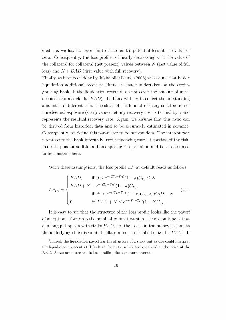
ered, i.e. we have a lower limit of the bank’s potential loss at the value of
zero. Consequently, the loss profile is linearly decreasing with the value of
the collateral for collateral (net present) values between N (last value of full
loss) and N + EAD (first value with full recovery).
Finally, as have been done by Jokivuolle/Peura (2003) we assume that beside
liquidation additional recovery efforts are made undertaken by the credit-
granting bank. If the liquidation revenues do not cover the amount of unre-
deemed loan at default (EAD), the bank will try to collect the outstanding
amount in a different vein. The share of this kind of recovery as a fraction of
unredeemed exposure (scarp value) net any recovery cost is termed by γ and
represents the residual recovery rate. Again, we assume that this ratio can
be derived from historical data and so be accurately estimated in advance.
Consequently, we define this parameter to be non-random. The interest rate
r represents the bank-internally used refinancing rate. It consists of the risk-
free rate plus an additional bank-specific risk premium and is also assumed
to be constant here.
With these assumptions, the loss profile LP at default reads as follows:
LPTD=
EAD, if 0 ≤ e−r(TL−TD)(1− k)CTL≤ N
EAD +N − e−r(TL−TD)(1− k)CTL,
if N < e−r(TL−TD)(1− k)CTL< EAD +N
0, if EAD +N ≤ e−r(TL−TD)(1− k)CTL.
(2.1)
It is easy to see that the structure of the loss profile looks like the payoff
of an option. If we drop the nominal N in a first step, the option type is that
of a long put option with strike EAD, i.e. the loss is in-the-money as soon as
the underlying (the discounted collateral net cost) falls below the EAD4. If
4Indeed, the liquidation payoff has the structure of a short put as one could interpret
the liquidation payment at default as the duty to buy the collateral at the price of the
EAD. As we are interested in loss profiles, the signs turn around.
10

we additionally take the nominal into account, we have an offsetting position
for collateral values between zero and N , i.e. a short put with strike N . The
combined position is that of a bear put spread.
The expected loss given default is given by the expected loss profile related
to the total exposure and multiplied by 1 − γ which accounts for residual
recovery:
E[LGDTD] = (1− γ)
1
EADE[LPTD
|τ = TD], (2.2)
where we have E[LGDTD] = E[LGD|D = 1] and τ is the set of all possible
times of default. For the special case where N = 0 (no senior positions) and
TD = TL (no liquidation delay) we obtain
E[LGDTD] = (1− γ)
1
EADE[max(EAD − (1− k)CTD
, 0)|τ = TD]
= (1− γ)E[EADNC
EAD|τ = TD
]. (2.3)
Here, the parameter EADNC represents the non-collateralized share of the
unredeemed loan. For fully uncollateralized loans, we have EADNC = EAD,
so that the LGD is only driven by the residual recovery process.
For the remainder of the article, we assume collateralized credit engage-
ments. Treating the exposure at default as non-random, the only random
factor influencing the loss profile and therefore the loss given default, is the
value of the collateral. Focussing on residential or commercial property,
we model the value of the collateral as an exponential Ornstein-Uhlenbeck-
process (OU) as motivated above. Moreover, we assume that the market
value of the collateral asset can be represented at any point in time T > t as
CT = CteYT , (2.4)
where YT is an OU-process. As noted above, the exponential OU-process
was proposed by Fabozzi/Shiller/Tunaru (2012) for the development of real
estate property values and captures characteristic features of the housing
market:
11
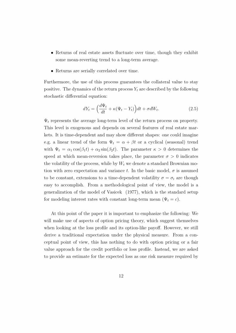
• Returns of real estate assets fluctuate over time, though they exhibit
some mean-reverting trend to a long-term average.
• Returns are serially correlated over time.
Furthermore, the use of this process guarantees the collateral value to stay
positive. The dynamics of the return process Yt are described by the following
stochastic differential equation:
dYt =(dΨt
dt+ κ(Ψt − Yt)
)dt+ σdWt. (2.5)
Ψt represents the average long-term level of the return process on property.
This level is exogenous and depends on several features of real estate mar-
kets. It is time-dependent and may show different shapes: one could imagine
e.g. a linear trend of the form Ψt = α + βt or a cyclical (seasonal) trend
with Ψt = α1 cos(β1t) + α2 sin(β2t). The parameter κ > 0 determines the
speed at which mean-reversion takes place, the parameter σ > 0 indicates
the volatility of the process, while by Wt we denote a standard Brownian mo-
tion with zero expectation and variance t. In the basic model, σ is assumed
to be constant, extensions to a time-dependent volatility σ = σt are though
easy to accomplish. From a methodological point of view, the model is a
generalization of the model of Vasicek (1977), which is the standard setup
for modeling interest rates with constant long-term mean (Ψt = c).
At this point of the paper it is important to emphasize the following: We
will make use of aspects of option pricing theory, which suggest themselves
when looking at the loss profile and its option-like payoff. However, we still
derive a traditional expectation under the physical measure. From a con-
ceptual point of view, this has nothing to do with option pricing or a fair
value approach for the credit portfolio or loss profile. Instead, we are asked
to provide an estimate for the expected loss as one risk measure required by
12

the Basle Committee5. Consequently, the fact that the real estate market
is incomplete – which is important when valuing real estate derivatives (see
Fabozzi/Shiller/Tunaru (2012)) – does not play a major role here. Math-
ematically speaking, that means that there is no change of measure or risk
premium here. Furthermore, the idea of discounting the future claim to to-
day is not appropriate when thinking of the future loss at default time TD
that can be expected today.
It is straightforward to show that for all t < T the solution of equation
(2.5) is given by
YT = ΨT − (Ψt − Yt)e−κ(T−t) + σ
∫ T
t
e−κ(T−s)dWs. (2.6)
Obviously, YT is a Gaussian process with the following conditional moments:
E[YT | Yt] = ΨT − (Ψt − Yt)e−κ(T−t) (2.7)
V ar[YT | Yt] =σ2
2κ
(1− e−2κ(T−t)
). (2.8)
As one should expect, for the long-term limit we obtain
limT→∞
E[YT | Yt] = Ψ∞
while the long-term variance is
limT→∞
V ar[YT | Yt] =σ2
2κ.
We state that even though the expected value can increase without any
bound depending on the shape of Ψ, the variance remains limited. Two
more interesting features of the process have to do with the parameter κ.
We have
limκ→∞
E[YT | Yt] = ΨT
5Though an isolated view on this measure may be misleading, in combination with
other risk measures (e.g. value at risk) the information may nevertheless prove useful.
13

limκ→∞
V ar[YT | Yt] = 0
as well as
limκ→0
E[YT | Yt] = ΨT −Ψt + Yt
limκ→0
V ar[YT | Yt] = σ2(T − t).
For an infinite speed of mean-reversion, the return process becomes deter-
ministic. For κ = 0 however, there is no feedback between the current level
of return Yt and the number Ψt, we have a classical Brownian motion plus a
deterministic drift component.
We conclude this section by bringing the results from the return to the
price level of the collateral. We receive
E[CT | Ct] = CteµY + 1
2σ2Y (2.9)
V ar[CT | Ct] = C2t e
2µY +σ2Y (eσ
2Y − 1), (2.10)
where µY = µYTand σ2
Y = σ2YT
are the moments of the return process YT
given by equations (2.7) and (2.8). Additionally, we observe the probability
that the collateral value CT exceeds a critical value x is given by
P (CT > x) = Φ(d), (2.11)
with d = (ln(Ct/x) + µY )/σY and Φ(x) is the standard normal distribution
at point x, i.e.
Φ(x) =1√2π
∫ x
−∞e−
12z2dz.
With limx→0 d = ∞, we obtain P (CT > 0) = 1, i.e. the value of the collateral
cannot become negative.
14

3 The expected loss given default
In this section we derive an analytical solution for the expected loss given
default. With the model setup of the previous section and the related as-
sumptions, the LGD is influenced by a couple of parameters and we can
write
E[LGDTD] = E[LGDTD
(EAD,N,C, k, TD, TL, γ, r,Ψ, κ, σ)].
We start by providing the main result concerning the expected loss given
default:
Theorem 3.1 As of time t, the expected loss given default for an obligor
defaulting at time TD is given by
E[LGDTD] = (1− γ)
[(1 +
N
EAD
)Φ(−d)− N
EADΦ(−d∗)
−(1− k)e−r(TL−TD) Ct
EADeµY + 1
2σ2Y
[Φ(−(d+ σY ))− Φ(−(d∗ + σY ))
]],
(3.1)
where
d =ln Ct
X+ µY
σY
(3.2)
d∗ =ln Ct
X∗ + µY
σY
(3.3)
X =EAD +N
1− ker(TL−TD) (3.4)
X∗ =N
1− ker(TL−TD) (3.5)
µY = µYTL= ΨTL
− (Ψt − Yt)e−κ(TL−t) (3.6)
σ2Y = σ2
YTL=
σ2
2κ
(1− e−2κ(TL−t)
), (3.7)
and Φ(·) being the cumulative density function of the standard normal dis-
tribution.
15

For the proof, see Appendix A1.
Remark 3.2 In the special case where N = 0, i.e. d.h. the bank is the only
senior rank creditor, the formula for the LGD can be simplified as follows:
E[LGDTD] = (1−γ)
[Φ(−d)−(1−k)e−r(TL−TD) Ct
EADeµY + 1
2σ2Y Φ(−(d+σY ))
],
(3.8)
where d, µY and σY are as above while X = EAD/(1−k)er(TL−TD) is adjusted.
The formulae satisfy an economically interesting homogeneity condition.
Proposition 3.3 For any π > 0 we have
E[LGDTD(πEAD, πN, πC, k, TD, TL, γ, r,Ψ, κ, σ)]
= E[LGDTD(EAD,N,C, k, TD, TL, γ, r,Ψ, κ, σ)], (3.9)
e.g., the expected loss given default is homogeneous of degree zero with respect
to EAD,N and C.
The proof is an immediate consequence of equations (3.1)-(3.5). The eco-
nomical statement of this mathematical finding is that for the LGD only
the relationship between the three parameters matters, while absolute values
have no influence. This ensures that all obligors are considered in the same
way (especially, independent of the firm size).
We investigate the analytic structure of the derived formula a little deeper.
For the purpose of a better understanding, we look at some examples based
on concrete numbers. First, we analyze graphically, how the rank structure
influences the expected LGD. We compare two cases of loans with even char-
acteristics except that the first loan exhibits a senior position of a third party
amounting to a nominal of N = 50, whereas in the second case this is not the
case (N = 0). We let the long-term mean of real estate returns be constant
at a level of Ψt = 0.06 and choose the other parameters as follows: EAD =
16

0 20 40 60 80 100 120 140 160 1800
0.1
0.2
0.3
0.4
0.5
0.6
0.7
0.8
Collateral C
Exp
ecte
d L
GD
N = 50N = 0
Figure 1: LGD estimates for two different tranches.
100, TD = 1, TL = 1.5, k = 0.05, r = 0.05, Y = 0.04, γ = 0.25, κ = 2, σ = 0.3.
The expected LGD depending on today’s value of the collateral is depicted
in Figure 1 for both cases.
As expected, in both cases, the expected LGD is decreasing with increas-
ing values of the collateral. The main difference, however, is that for the first
scenario the existence of the third-party nominal (N = 50) shifts the LGD
values considerably upwards. As long as the collateral only suffices to serve
the senior position, there is no recovery from the liquidation. In our model,
the residual recovery process characterized by the parameter γ = 25% limits
the loss to a maximum of 75%.
We now relax the assumptions assuming a linear trend for the long-term
mean of returns on residential property, i.e. Ψt = α+ βt. Again, we choose
two different scenarios: one scenario where the housing market is prospering,
the other scenario where it diminishes. The values for the scenarios are given
in Table 1.
The other parameters that are equal for both cases are: TD = 1, EAD =
17
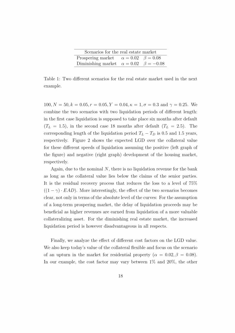
Scenarios for the real estate marketProspering market α = 0.02 β = 0.08Diminishing market α = 0.02 β = −0.08
Table 1: Two different scenarios for the real estate market used in the next
example.
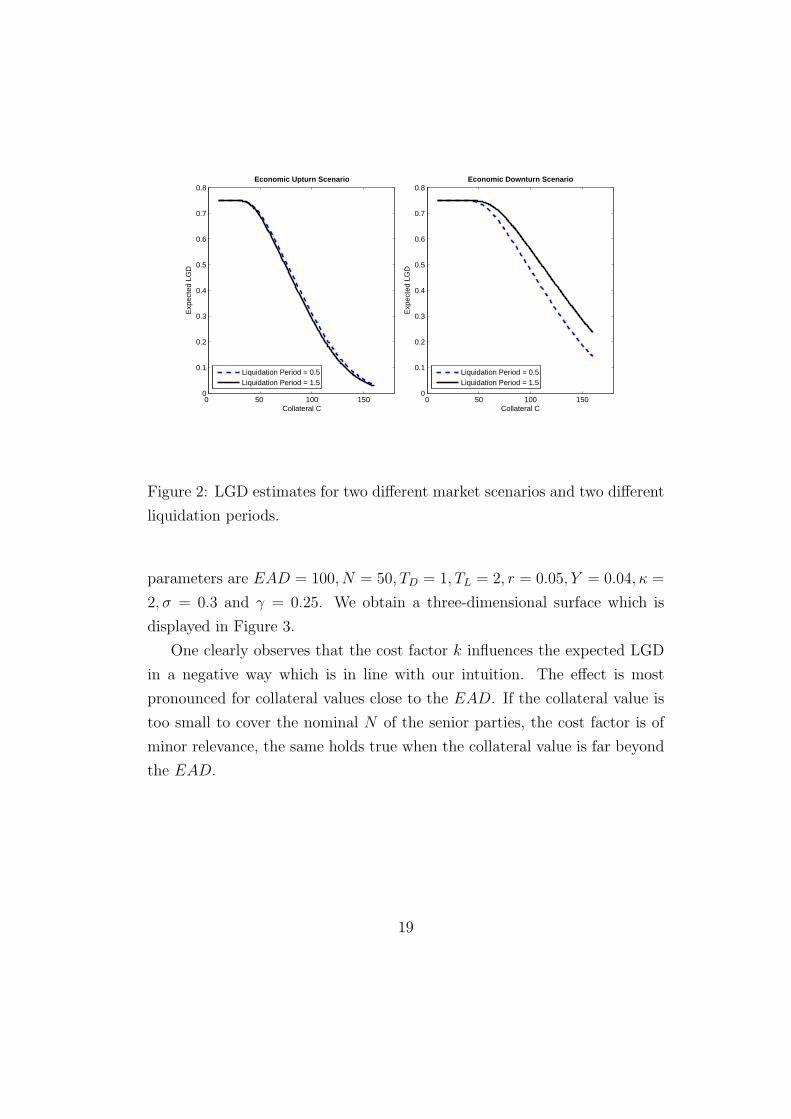
100, N = 50, k = 0.05, r = 0.05, Y = 0.04, κ = 1, σ = 0.3 and γ = 0.25. We
combine the two scenarios with two liquidation periods of different length:
in the first case liquidation is supposed to take place six months after default
(TL = 1.5), in the second case 18 months after default (TL = 2.5). The
corresponding length of the liquidation period TL − TD is 0.5 and 1.5 years,
respectively. Figure 2 shows the expected LGD over the collateral value
for these different speeds of liquidation assuming the positive (left graph of
the figure) and negative (right graph) development of the housing market,
respectively.
Again, due to the nominal N , there is no liquidation revenue for the bank
as long as the collateral value lies below the claims of the senior parties.
It is the residual recovery process that reduces the loss to a level of 75%
((1− γ) ·EAD). More interestingly, the effect of the two scenarios becomes
clear, not only in terms of the absolute level of the curves: For the assumption
of a long-term prospering market, the delay of liquidation proceeds may be
beneficial as higher revenues are earned from liquidation of a more valuable
collateralizing asset. For the diminishing real estate market, the increased
liquidation period is however disadvantageous in all respects.
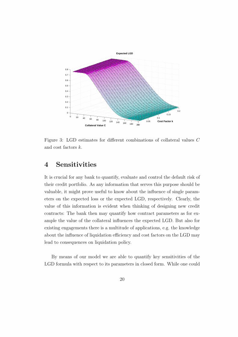
Finally, we analyze the effect of different cost factors on the LGD value.
We also keep today’s value of the collateral flexible and focus on the scenario
of an upturn in the market for residential property (α = 0.02, β = 0.08).
In our example, the cost factor may vary between 1% and 20%, the other
18
0 50 100 1500
0.2
0.4
0.6
0.8
0.1
0.3
0.5
0.7
Economic Upturn Scenario
Collateral C
Exp
ecte
d LG
D
0 50 100 1500
0.1
0.2
0.3
0.4
0.5
0.6
0.7
0.8Economic Downturn Scenario
Collateral CE
xpec
ted
LGD
Liquidation Period = 0.5Liquidation Period = 1.5
Liquidation Period = 0.5Liquidation Period = 1.5
Figure 2: LGD estimates for two different market scenarios and two different
liquidation periods.
parameters are EAD = 100, N = 50, TD = 1, TL = 2, r = 0.05, Y = 0.04, κ =
2, σ = 0.3 and γ = 0.25. We obtain a three-dimensional surface which is
displayed in Figure 3.
One clearly observes that the cost factor k influences the expected LGD
in a negative way which is in line with our intuition. The effect is most
pronounced for collateral values close to the EAD. If the collateral value is
too small to cover the nominal N of the senior parties, the cost factor is of
minor relevance, the same holds true when the collateral value is far beyond
the EAD.
19
0 20 40 60 80 100 120 140 160 180 2000
0.05
0.1
0.15
0.20
0.1
0.2
0.3
0.4
0.5
0.6
0.7
0.8
Cost Factor k
Expected LGD
Collateral Value C
Figure 3: LGD estimates for different combinations of collateral values C
and cost factors k.
4 Sensitivities
It is crucial for any bank to quantify, evaluate and control the default risk of
their credit portfolio. As any information that serves this purpose should be
valuable, it might prove useful to know about the influence of single param-
eters on the expected loss or the expected LGD, respectively. Clearly, the
value of this information is evident when thinking of designing new credit
contracts: The bank then may quantify how contract parameters as for ex-
ample the value of the collateral influences the expected LGD. But also for
existing engagements there is a multitude of applications, e.g. the knowledge
about the influence of liquidation efficiency and cost factors on the LGD may
lead to consequences on liquidation policy.
By means of our model we are able to quantify key sensitivities of the
LGD formula with respect to its parameters in closed form. While one could
20

investigate influence of any model parameter, we focus on an (in our opinion)
appropriate choice of the most important ones.
The first sensitivity we derive is the one with respect to the value of the
collateral C, which – in analogy to option pricing theory – we name Delta:
Proposition 4.1 For the Delta of the expected LGD (Theorem 3.1) it holds:
∂E[LGDTD]
∂C= (1− γ)
[− n(d)
σY · C+
N
EAD · σY · C(n(d∗)− n(d))
−(1− k)e−r(TL−TD) eµY + 1
2σ2Y
EAD
[Φ(−(d+ σY ))− Φ(−(d∗ + σY ))
+1
σY
(n(d∗ + σY )− n(d+ σY ))]], (4.1)
where Φ(·) are the cumulative density function and n(·) the density function
of the standard normal distribution.
For the proof, see Appendix A2.
Remark 4.2 For the special case N = 0 (no other senior positions), the
formula for the Delta can be written as
∂E[LGDTD]
∂C= (1−γ)
[− n(d)
σY · C−(1−k)e−r(TL−TD) e
µY + 12σ2Y
EAD
[Φ(−(d+σY ))−
n(d+ σY )
σY
]],
(4.2)
where we have X = EAD/(1− k)er(TL−TD).
For a graphical illustration we use the same example as in the previous
section (Figure 1) where we had the case with a nominal N = 50 as well
as without any nominal N = 0. For ease of interpretation, we exclude the
residual recovery actions here setting γ = 0. The other parameter values were
EAD = 100, TD = 1, TL = 1.5, k = 0.05, r = 0.05, Y = 0.04, κ = 2, σ = 0.3
and Ψt = 0.06. Figure 4 depicts the Delta values for the two cases over the
collateral value.
21

0 20 40 60 80 100 120 140 160 180 200−0.01
−0.009
−0.008
−0.007
−0.006
−0.005
−0.004
−0.003
−0.002
−0.001
0
Collateral C
Exp
ecte
d L
GD
Del
ta
N = 50N = 0
Figure 4: LGD Delta estimates for two different tranches.
Obviously, if the lending bank is in senior position (N = 0), the delta is
at a constant level of minus one percentage point for very low collateral val-
ues. This value results from the fact that an increase of the collateral value
by one unit also reduces the expected loss in total amounts by (almost) one
unit. Divided by the EAD, which is 100 in this example, we receive the
effect on the expected loss rate there to be -1%. With the analogy to option
pricing stated above, recall that the payoff profile of LGD without nominal
N resembles the position of a long put. For a collateral value close to zero,
this option is far in-the-money. With increasing value of the collateral, the
reduction on the expected loss is lower and finally tends to a level of zero for
high collateral values. Here, the put option is far out-of the money, so that
a further increase of the underlying value has nearly no effect on the value
of the option.
If a third-party senior position exists with a nominal, there is an addi-
tional effect. For very low collateral values, the effect on the expected LGD
is close to zero: Here, an increase of the collateral’s value only helps the first-
22
tier creditors because the probability of any liquidation revenue that exceeds
the nominal is rather low. Coming closer to the nominal, the potential loss
reduction strengthens more and more. After exceeding the nominal value we
have a shifted version of the first case described above: from the maximum
effect of -1.00%, a further increase of the collateral’s value will first result in
weaker effects and finally fade out. Once more making use of option theory
terminology, the LGD profile can be described as a combination of a short
put with strike N = 50 and a long put with strike N + EAD = 150 (i.e. a
bear put spread): For low collateral values, both options are far in-the-money
and the effects (+1% for the short put and -1% for the long put) offset each
other. Approaching the strike of the short put, the potential effect of the
short put decreases from the value of +1% to zero while the long put is still
far in-the money with a delta of -1% dominates, the sum of the two therefore
evolves from 0 to -1%. With the collateral’s value increasing further, the
short put loses any influence and we have the shape of the long put’s delta
as in the example without any senior third-party.
The second sensitivity we investigate more deeply is the partial derivative
of the expected loss given default with respect to the time of liquidation TL:
23
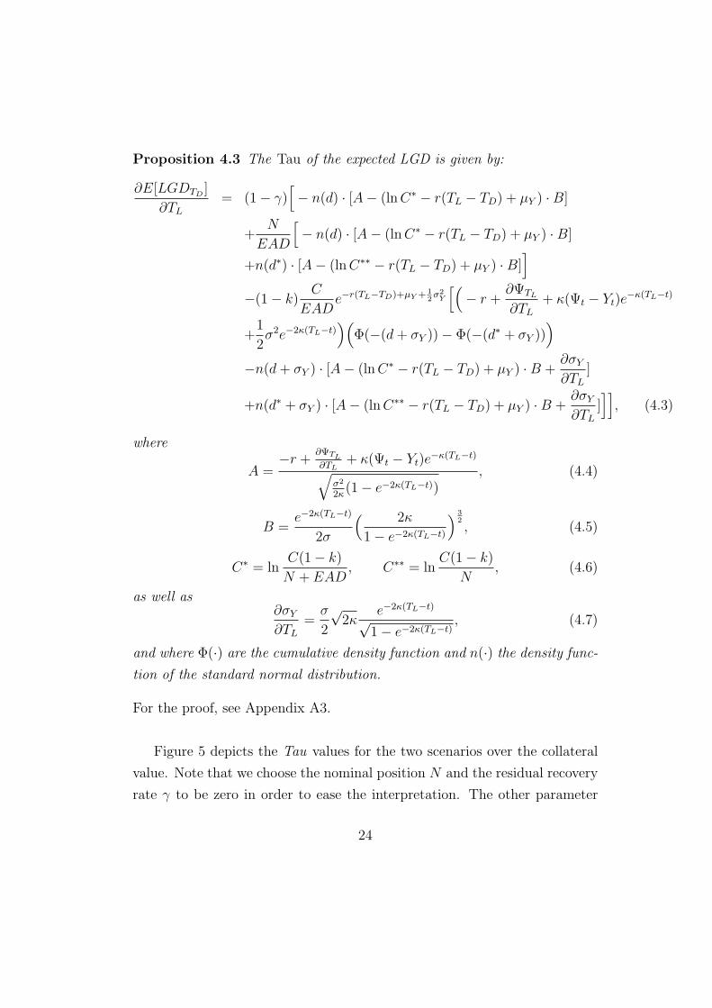
Proposition 4.3 The Tau of the expected LGD is given by:
∂E[LGDTD]
∂TL
= (1− γ)[− n(d) · [A− (lnC∗ − r(TL − TD) + µY ) ·B]
+N
EAD
[− n(d) · [A− (lnC∗ − r(TL − TD) + µY ) ·B]
+n(d∗) · [A− (lnC∗∗ − r(TL − TD) + µY ) ·B]]
−(1− k)C
EADe−r(TL−TD)+µY + 1
2σ2Y
[(− r +
∂ΨTL
∂TL
+ κ(Ψt − Yt)e−κ(TL−t)
+1
2σ2e−2κ(TL−t)
)(Φ(−(d+ σY ))− Φ(−(d∗ + σY ))
)−n(d+ σY ) · [A− (lnC∗ − r(TL − TD) + µY ) ·B +
∂σY
∂TL
]
+n(d∗ + σY ) · [A− (lnC∗∗ − r(TL − TD) + µY ) ·B +∂σY
∂TL
]]], (4.3)
where
A =−r +
∂ΨTL
∂TL+ κ(Ψt − Yt)e
−κ(TL−t)√σ2
2κ(1− e−2κ(TL−t))
, (4.4)
B =e−2κ(TL−t)
2σ
( 2κ
1− e−2κ(TL−t)
) 32, (4.5)
C∗ = lnC(1− k)
N + EAD, C∗∗ = ln
C(1− k)
N, (4.6)
as well as∂σY
∂TL
=σ
2
√2κ
e−2κ(TL−t)
√1− e−2κ(TL−t)
, (4.7)
and where Φ(·) are the cumulative density function and n(·) the density func-
tion of the standard normal distribution.
For the proof, see Appendix A3.
Figure 5 depicts the Tau values for the two scenarios over the collateral
value. Note that we choose the nominal position N and the residual recovery
rate γ to be zero in order to ease the interpretation. The other parameter
24

values are EAD = 100, TD = 1, TL = 2.5, k = 0.05, r = 0.05, Y = 0.04, κ = 2
and σ = 0.3 .
0 50 100 150 200−0.1
−0.09
−0.08
−0.07
−0.06
−0.05
−0.04
−0.03
−0.02
−0.01
0Economic Upturn Scenario
Collateral C
Exp
ecte
d L
GD
Tau
0 50 100 150 2000
0.05
0.1
0.15
0.2
0.25
0.3
0.35
0.4
0.45Economic Downturn Scenario
Collateral C
Exp
ecte
d L
GD
Tau
Figure 5: LGD Tau estimates for two different market scenarios.
As already suggested by Figure 2, the effect observable in this example
heavily depends on the choice of the long-term mean ΨTL, yielding a decrease
in loss and hence a negative Tau for an upward-tending real estate market
and vice versa. For both scenarios, the absolute value of the partial derivative
takes a maximum value in the vicinity of the EAD. As goes along with intu-
ition, for highly collateralized engagements (C >> EAD), the fluctuations
of the collateral value induced by the prolongation of time play a dwindling
role.
25

5 Conclusion
In this paper, we derived closed-form solutions for the loss given default
(LGD) quotas. We therefor focussed on a selected subcase of LGD where
loans of the retail sector are collateralized by residential or commercial real
estate property. In our opinion, this specification is feasible and reasonable
in more than one regards: first, it is one of the most important cases for
the retail sector, second, it facilitates the disentanglement of PD and LGD
which makes computations tractable and third, it allows for a case-specific
and powerful modeling of the collateral value. To the best of our knowledge,
the (careful) use of option pricing analogies with respect to methodology
and interpretation of sensitivities has not been worked out before in that
clearness. For sake of broad applicability, we incorporated typical problems
of practitioners’ workaday life like cost factors, residual recovery, liquidation
periods and existing third-party nominal. Still being in a handy size, we
hope that the formulae is attractive for practitioners with useful tools as
sensitivities and intuition-feeding graphical illustrations. On the other hand,
it may be a starting point for researchers to develop further sector-specific
LGD formulae based on option-pricing arguments.
A Appendix
A.1
Proof of Theorem 3.1: First, we note that E[LPTD|τ = TD] may be written
as
E[LPTD|τ = TD] = E[max(E +N − e−r(TL−TD)(1− k)CTL
, 0)]
−E[max(N − e−r(TL−TD)(1− k)CTL, 0)]. (A.1)
Furthermore, we know that the return process YTL(conditioned on Yt) is a
normal variable with expectation µY and variance σ2Y given in Theorem 3.1.
26

Hence the density function of the collateral CTLequals
p(CTL|Ct) =
1
CTL
√2πσ2
Y
exp(− 1
2
( lnCTL− (lnCt + µY )
σY
)2). (A.2)
The calculation of the expected loss profile as a sum of two expectations is
done straightforwardly and is left as an exercise. The result is the formula
stated in the Theorem. �
A.2
The proof of the formula for the delta is done fairly easy. We treat the
parameter d and d∗ as functions of C and get
∂d(C)
∂C=
∂d∗(C)
∂C=
1
σY · C. (A.3)
Applying the chain rule for derivatives we obtain
∂Φ(−d)
∂C= − n(d)
σY · C, (A.4)
and∂Φ(−d∗)
∂C= − n(d∗)
σY · C. (A.5)
A straightforward application of the product rule establishes the formula. �
A.3
The derivation of the sensitivity formula with respect to the parameter TL is
slightly more cumbersome. Similarly to the delta case, we treat the variables
d, d∗, µY and σY as function of TL. We have
d(TL) =lnC∗ − r(TL − TD) + µY (TL)
σY (TL), (A.6)
where C∗ = ln(C(1− k)/(N + EAD)) (analogously for d∗). Further,
∂µ(TL)
∂TL
=∂ΨTL
∂TL
+ κ(Ψt − Yt)e−κ(TL−t), (A.7)
27

and∂σY (TL)
∂TL
=σ
2
√2κ
e−2κ(TL−t)
√1− e−2κ(TL−t)
. (A.8)
Application of the chain rule gives
∂Φ(−d)
∂C= −n(d)
∂d(TL)
∂TL
(A.9)
(analogously for d∗). The final expression follows after applying and combin-
ing the product and quotient rule for derivatives and aggregation. �
References
V.V. Acharya, S.T. Bharath and A. Srinivasan, Does industry-wide distress
affect defaulted firms? Evidence from creditor recoveries, Journal of Fi-
nancial Economics, Vol. 85, 2007, pp. 787-821.
E.I. Altman, A. Resti and A. Sironi, Analyzing and Explaining Default Re-
covery Rates, ISDA Research Report, London, 2001.
E.I. Altman, B. Brady, A. Resti and A. Sironi, The Link between Default and
Recovery Rates: Theory, Empirical Evidence and Implications, Journal of
Business, Vol. 78 (6), 2005, pp. 2203-27.
B. Bade, D. Rosch and H. Scheule, Default and Recovery Risk Dependencies
in a Simple Credit Risk Model, European Financial Management, Vol. 17
(1), 2011, pp. 120-144.
T. Bjork and E. Clapham, On the pricing of real estate index linked swaps,
Journal of Housing Economics, Vol. 11 (4), 2002, pp. 418-432.
R.J. Buttimer Jr, J.B. Kau, and V.C. Slawson Jr., A model for pricing secu-
rities dependent upon a real estate index, Journal of Housing Economics,
Vol. 6 (1), 1997, pp. 16-30.
28
M. Cao and J. Wei, Valuation of Housing Index Derivatives, Journal of Fu-
tures Markets, Vol. 30 (7), 2010, pp. 660-688.
K.E. Case, R.J. Shiller, The efficiency of the market for single-family homes,
The American Economic Review, Vol. 79 (1), 1989, pp. 125-137.
K.E. Case, R.J. Shiller, Forecasting prices and excess returns in the housing
market, Real Estate Economics, Vol. 18 (3), 1990, pp. 253-273.
S. Caselli, S. Gatti and F. Querci, The sensitivity of the loss given default
rate to systematic risk: new empirical evidence on banl loans, Journal of
Financial Services Research, Vol. 34 (1), 2008, pp. 1-34.
P. Ciurlia and A. Gheno, A model for pricing real estate derivatives with
stochastic interest rates, Mathematical and Computer Modelling, Vol. 50
(1), 2009, pp. 233-247.
G.W. Crawford and M.C. Fratantoni (2003), Assessing the Forecasting Per-
formance of Regime-Switching, ARIMA and GARCH Models of House
Prices, Real Estate Economics, Vol. 31 (2), 2003, pp. 223-243.
A. Dev and M. Pykhtin, Analytical approach to credit risk modelling, Risk,
March 2002, pp. 26-32.
A. Dıaz and B. Jerez, House Prices, Sales, And Time On The Market: A
Search-Theoretic Framework, International Economic Review, Vol. 54 (3),
2013, pp. 837-872.
P. Englund and Y.M. Ioannides, House price dynamics: an international
empirical perspective, Journal of Housing Economics, Vol. 6 (2), 1997, pp.
119-136.
F.J. Fabozzi, R.J. Shiller and R.S. Tunaru, Property Derivatives for Manag-
ing European Real-Estate Risk, European Financial Management, Vol. 16
(1), 2010, pp. 8-26.
29

F.J. Fabozzi, R.J. Shiller and R.S. Tunaru, A Pricing Framework for Real
Estate Derivatives, European Financial Management, Vol. 18 (5), 2012,
pp. 762-789.
J. Franks, A. de Servigny and S. Davydenko, A comparative analysis of
the recovery process and recovery rates for private companies in the U.K.,
France, and Germany, Standard and poor’s risk solutions, 2004.
J. Frye, Collateral Dammage, Risk, April 2000, pp. 91-94.
D. Geltner, J.D. Fisher, Pricing and index considerations in commercial real
estate derivatives, The Journal of Portfolio Management, Vol. 33 (5), 2007,
pp. 99-118.
J. Grunert, Verwertungserlose von Kreditsicherheiten: Eine empirische Anal-
yse notleidender Unternehmenskredite, Zeitschrift fur Betriebswirtschaft,
Vol. 80, 2010, pp. 1305-1323.
J. Grunert and M. Weber, Recovery rates of commercial lending: Empirical
evidence for German companies, Journal of Banking & Finance, Vol. 33,
2009, pp. 505-513.
M. Gurtler and M. Hibbeln, Improvements in loss given default forecasts for
bank loans, Journal of Banking & Finance, Vol. 37, 2013, pp. 2354-2366.
M. Hillebrand, Modeling and estimating dependent loss given default, Work-
ing Paper TU Munchen, 2005.
A.J. Hosios, J.E. Pesando, Measuring prices in resale housing markets in
Canada: evidence and implications, Journal of Housing Economics, Vol. 1
(4), 1991, pp. 303-317.
C. Hott, Lending behavior and real estate prices, Journal of Banking & Fi-
nance, Vol. 35 (9), 2011, pp. 2429-2442.
30
Y. Hu and W. Perraudin, The Dependence of Recovery Rates and Defaults,
Risk Control Research Paper No. 6/1 , 2006.
M. Jacobs Jr., Empirical Implementation of a 2-Factor Structural Model for
Loss-Given-Default, Cass-Capco Institute Paper Series on Risk, 2011.
E. Jokivuolle, Pricing European options on autocorrelated indexes, The Jour-
nal of Derivatives, Vol. 6 (2), 1998, pp. 39-52.
E. Jokivuolle and S. Peura, Incorporating Collateral Value Uncertainty in
Loss Given Default Estimates and Loan-to-value Ratios, European Finan-
cial Management, Vol. 9 (3), 2003, pp. 299-314.
J. Krainer, A theory of liquidity in residential real estate markets, Journal of
Urban Economics, Vol. 49 (1), 2001, pp. 32-53.
A.W. Lo, J. Wang, Implementing option pricing models when asset returns
are predictable, The Journal of Finance, Vol. 50 (1), 1995, pp. 87-129.
J. Perello, R. Sircar and J. Masoliver, Option pricing under stochastic volatil-
ity: the exponential Ornstein-Uhlenbeck model, Journal of Statistical Me-
chanics: Theory and Experiment, Vol. 6 , 2008, pp. 1-22.
R. Novy-Marx, Hot and Cold Markets, Real Estate Economics, Vol. 37 (1),
2009, pp. 1-22.
M. Piazzesi and M. Schneider, Momentum traders in the housing market:
survey evidence and a search model, Working paper No.w14669, National
Bureau of Economic Research, 2009.
M. Pykhtin, Unexpected recovery risk, Risk, August 2003, pp. 74-78.
S. Titman and W. Torous, Valuing Commercial Mortgages: An Empirical
Investigation of the Contingent-Claims Approach to Pricing Risky Debt,
The Journal of Finance, Vol. 44 (2), 1989, pp. 345-373.
31
G. Van Damme, A generic framework for stochastic Loss-Given-Default,
Journal of Computational and Applied Mathematics, Vol. 235, 2011, pp.
2523-2550.
O. Vasicek, An equilibrium characterization of the term structure, Journal of
financial economics, Vol.5 (2), pp. 177-188.
W.C. Wheaton, Vacancy, search, and prices in a housing market matching
model, Journal of Political Economy, Vol. 98 (6), 1990, pp. 1270-1292.
32