Estimating evolutionary parameters for Neisseria meningitidis Based on the Czech MLST dataset

Estimating evolutionary parameters for

Neisseria meningitidis

Based on the Czech MLST dataset

Testing a model of evolution: what you need

Starting sequence

Mutational model

Evolved sequence

1

2

1

2

Codon usage frequencies

Mutational model of sequence evolution

Choose codons at random from the observed

distribution of codon usage

Estimate evolutionary parameters from the observed data

Statistically test for differences between simulated and observed

patterns of variation.3

3 Statistical test of hypothesis

Simulation Real Data

Estimating Codon Usage Frequencies

1

Estimating Codon Frequency Usage

Methods available:

• Empirical observation of the Z2491 genome

• Empirical observation of the MLST data

• Bayesian inference using the MLST data

Empirical observation of the Z2491 genome

Parkhill et al (2000) Complete DNA sequence of a serogroup A strain of Neisseria meningitidis Z2491. Nature 404: 502-506.

Nakamura et al (2000) Codon usage tabulated from the international DNA sequence databases: status for the year 2000. Nuc. Acids Res. 28: 292.

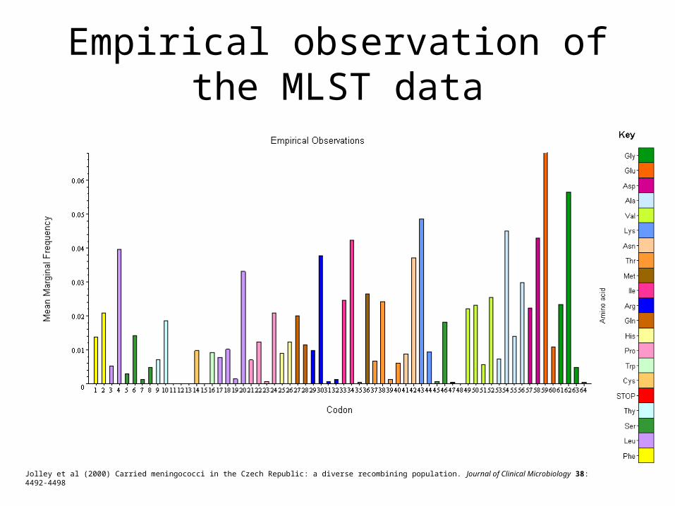
Empirical observation of the MLST data

Jolley et al (2000) Carried meningococci in the Czech Republic: a diverse recombining population. Journal of Clinical Microbiology 38: 4492-4498

Bayesian Inference

• Prior belief

In the absence of any information, what might you expect codon usage to look like a priori? E.g.

Codon frequency usage is unbiased and homogeneous, except for the stop codons which have

zero frequency, since the sequences are coding.

• Empirical data - tally the codon usage in the MLST dataset

• Posterior belief

Modify the prior beliefs a posteriori, following exposure to real data. The degree to which your

beliefs are modified depends on the conviction with which you held your prior beliefs. The

posterior beliefs will fall somewhere between the empirical observations and the prior beliefs. I.e.

the posterior distribution of codon usage will be a compromise between all non-stop codons

having some non-zero frequency and the observed empirical patterns of variation in codon

usage.

Assumptions made in the Bayesian Inference

• Refer to a triplet as a 3-base slot in the reading frame, and a codon as the

specific combination of bases filling that slot.

• Codon usage was modelled multinomially, i.e. each triplet is a random

draw from one of the 61 possible non-stop codons. This makes the following

assumptions:

– The presence of one or another codon at any particular triplet is entirely

independent of the codons at adjacent triplets.

– All triplets are identical with respect to the probable codon usage.

– We will never see any of the three STOP codons in our sequences.

A priori belief in codon frequency usage

Empirical observation of the MLST data

Jolley et al (2000) Carried meningococci in the Czech Republic: a diverse recombining population. Journal of Clinical Microbiology 38: 4492-4498

A posteriori belief in codon frequency usage

Mutational Model ofSequence Evolution

2

Phylogenetic Inference

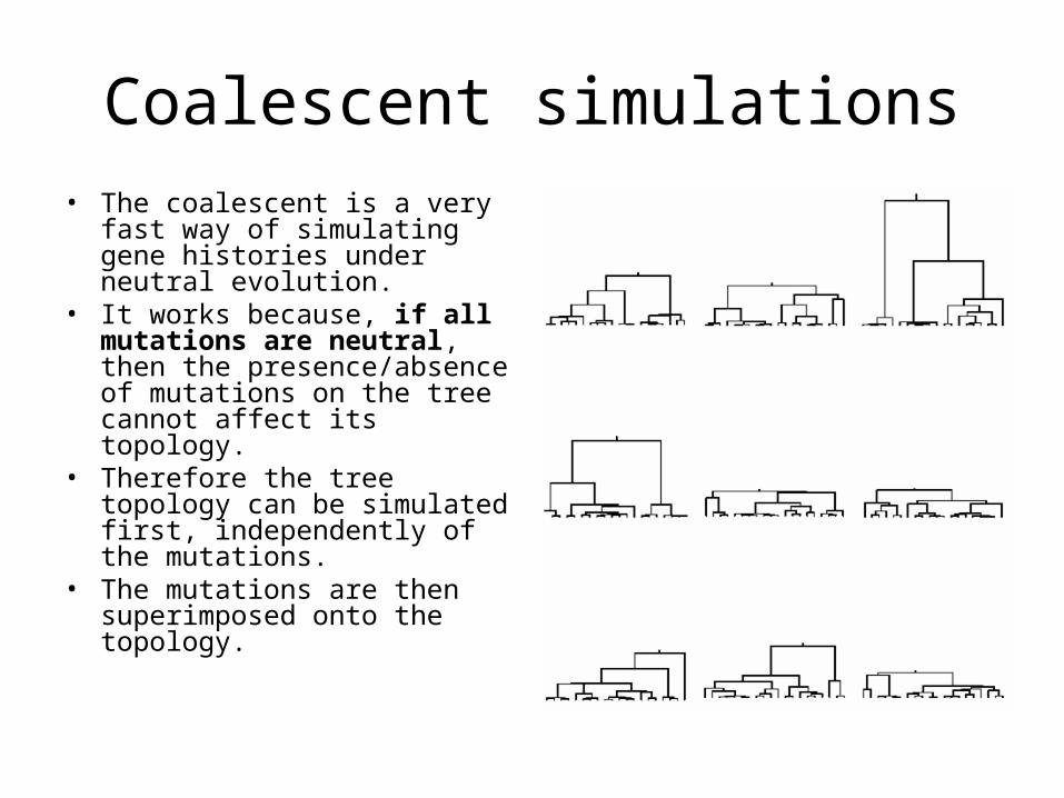
Coalescent simulations• The coalescent is a very fast

way of simulating gene histories under neutral evolution.

• It works because, if all mutations are neutral, then the presence/absence of mutations on the tree cannot affect its topology.

• Therefore the tree topology can be simulated first, independently of the mutations.

• The mutations are then superimposed onto the topology.

Underlying rates of non-synonymous mutation are usually confounded with selection against inviable mutants.

Thus it is convenient to model functional constraint as mutational bias.(Or rather, make no attempt to disentangle the two).

If we assume that the patterns of functional constraint can be modelled as a biased, but neutral, form of mutation, then we can use Coalescent simulation.

Ancestral type

Neutral mutant

Inviable mutant

Mutation Selection

Sampling usuallyoccurs at this point

Mutational bias in Coalescent Simulations

• The topology is simulated at random, as before.• As in normal coalescent simulations, mutations

are superimposed onto the topology according to a Poisson process (just as in the neutral model of molecular evolution).

• Those mutations, although assumed to be neutral, are biased.

• The types of mutations must therefore be classified to specify the bias.

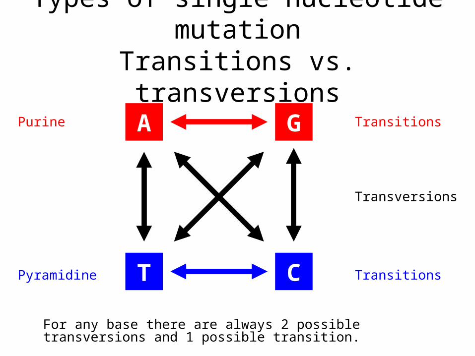
Types of single nucleotide mutationTransitions vs. transversions

A G

T C

Purine

Pyramidine Transitions

Transitions

Transversions

For any base there are always 2 possible transversions and 1 possible transition.

Types of codon mutationSynonymous vs. non-synonymous

T T G

T T A

Leucine

Leucine

T T G

A T G

Leucine

Methionine

LeucinepH 5.98

6-fold degeneracy in the genetic code

MethioninepH 5.74

Single unique codon ATG

(CH3)2-CH-CH2-CH(NH2)-COOHCH3-S-(CH2)2-CH(NH2)-COOH

Synonymous Non-synonymous

http://www.chemie.fu-berlin.de/chemistry/bio/aminoacid/mol/leu.mol

http://www.chemie.fu-berlin.de/chemistry/bio/aminoacid/mol/met.mol

Relative rates of the different classes of mutation

Rate of occurrence

Synonymous transversion

Synonymous transition

Non-synonymous transversion

Non-synonymous transition

Interpretation

Transition-transversion ratio

Proportion of non-synonymous mutations that are viable

Basic rate of mutation per codon

Example: CTT

C T T T TT TT T

T TT TT TT TT TT T

TAG

CAG

CAG

Phe Non-synonymous transition Ile Non-synonymous

transversion Val Non-synonymous

transversion Ser Non-synonymous transition Tyr Non-synonymous

transversion Cys Non-synonymous

transversion Phe Non-synonymous transition Leu Synonymous transversion Leu Synonymous transversion

Leucine

Likelihood

• Having defined the model of evolution, the probability of observing different patterns in the data can be expressed.

• The triplets in the MLST sequences are aligned, and the pattern of diversity in the sample at each triplet is analyzed.

• The number of mutations occurring in the gene history is Poisson distributed, according to the neutral theory, with rate equal to the basic mutation rate multiplied by the evolutionary time over which mutation could have occurred.

• Evolutionary time is obtained from Coalescent theory.• The basic mutation rate and the relative rates of each

type of mutation are estimated from the data.

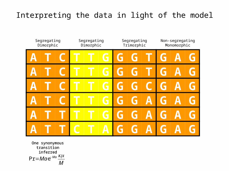
Interpreting the data in light of the model

A T CA T CA T CA T CA T TA T T

G A GG A GG A GG A GG A GG A G

T T GT T GT T GT T GT T GC T A

G G TG G TG G CG G AG G AG G A

SegregatingDimorphic

Non-segregatingMonomorphic


SegregatingTrimorphic












A T CA T TA T CA T T

Make the assumption that no more than a single mutation occurs anywhere in the tree since the most recent common ancestor.


A T CA T CA T TA T T

A T CA T C

A T C

A T CA T CA T TA T T

A T CA T C

A T T

Synonymous transition, rate

Synonymous transition, rate

For a dimorphic segregating triplet, on the assumption that no more than a single mutation has occurred, ancestral type is irrelevant.


From Coalescent Theory, the evolutionary time over which mutations can occur for a gene history of n genes is given by the Watterson constant:

1

1

12n

i ia

If M is the basic rate of mutation per codon and the number of mutations in the tree is Poisson distributed, then

Pr{0 mutations} = e-Ma

Pr{1 mutation} = Ma e-Ma

Pr{2 mutations} = (Ma)2e-Ma/2

Pr{3 mutations} = (Ma)3e-Ma/6










One synonymous transition inferred

MMa Ma ePr










One synonymous transition inferredOne synonymous transition inferred

MMa Ma ePr


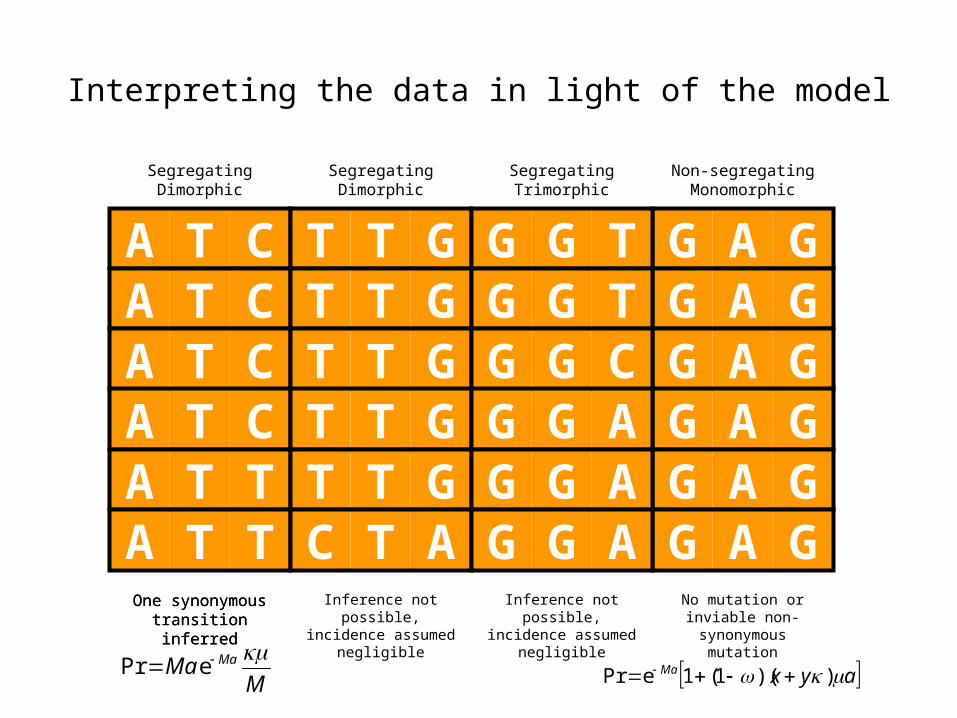
Under the assumption of no more than a single mutation this change cannot occur. Its frequency is assumed negligible, and any occurrences in the data are ignored.


T T GC T AT T GC T A











Inference not possible, incidence assumed negligible


MMa Ma ePr













MMa Ma ePr














MMa Ma ePr














MMa Ma ePr


1. Because there has been no mutation since the most recent common ancestor!

Pr = e-Ma

2. Because there has been an inviable non-synonymous mutation that was purged by selection

Pr = x(1-) Ma e-Ma/M

+ y(1-) Ma e-Ma/M

G A GG A GG A GG A G

G A GG A G

Why might a site be monomorphic?

Where x and y are the number of possible non-synonymous transversions and transitions respectively from codon GAG. Therefore

ayxMa ))(1(1ePr














MMa Ma ePr ayxMa ))(1(1ePr

No mutation or inviable non-synonymous

mutation


ayxMa ))(1(1ePr

aMaePr

aMa ePr

aMaePr

aMa ePr

Probability


Non-synonymous transversion

Non-synonymous transition

No change


Mutation type

Phe Phe Leu Leu Ser Ser Ser Ser Tyr Tyr STOPSTOP Cys Cys STOP Trp Leu Leu Leu Leu Pro Pro Pro Pro His His Gln Gln Arg Arg Arg Arg Ile Ile Ile Met Thr Thr Thr Thr Asn Asn Lys Lys Ser Ser Arg Arg Val Val Val Val A la Ala Ala Ala Asp Asp Glu Glu Gly Gly Gly GlyUUU UUC UUA UUG UCU UCC UCA UCG UAU UAC UAA UAG UGU UGC UGA UGG CUU CUC CUA CUG CCU CCC CCA CCG CAU CAC CAA CAG CGU CGC CGA CGG AUU AUC AUA AUG ACU ACC ACA ACG AAU AAC AAA AAG AGU AGC AGA AGG GUU GUC GUA GUG GCU GCC GCA GCG GAU GAC GAA GAG GGU GGC GGA GGG

1 2 3 4 5 6 7 8 9 10 11 12 13 14 15 16 17 18 19 20 21 22 23 24 25 26 27 28 29 30 31 32 33 34 35 36 37 38 39 40 41 42 43 44 45 46 47 48 49 50 51 52 53 54 55 56 57 58 59 60 61 62 63 64Phe UUU 1 1 3 4 4 5 4 0 0 4 0 5 4 4Phe UUC 2 1 4 4 5 4 0 0 4 0 5 4 4Leu UUA 3 1 3 5 4 0 4 2 4 4Leu UUG 4 1 5 0 4 0 4 2 4 4Ser UCU 5 1 3 2 2 4 0 0 4 0 5 4 4Ser UCC 6 1 2 2 4 0 0 4 0 5 4 4Ser UCA 7 1 3 4 0 4 5 4 4Ser UCG 8 1 0 4 0 4 5 4 4Tyr UAU 9 1 3 4 4 5 0 5 4 4Tyr UAC 10 1 4 4 5 0 5 4 4

STOP UAA 11 0 0 0 0 0 0 0 0 0 0 1 3 0 0 3 0 0 0 0 0 0 0 0 0 0 0 5 0 0 0 0 0 0 0 0 0 0 0 0 0 0 0 4 0 0 0 0 0 0 0 0 0 0 0 0 0 0 0 4 0 0 0 0 0STOP UAG 12 0 0 0 0 0 0 0 0 0 0 0 1 0 0 0 5 0 0 0 0 0 0 0 0 0 0 0 5 0 0 0 0 0 0 0 0 0 0 0 0 0 0 0 4 0 0 0 0 0 0 0 0 0 0 0 0 0 0 0 4 0 0 0 0Cys UGU 13 0 0 1 3 4 4 5 4 4Cys UGC 14 0 0 1 4 4 5 4 4

STOP UGA 15 0 0 0 0 0 0 0 0 0 0 0 0 0 0 1 5 0 0 0 0 0 0 0 0 0 0 0 0 0 0 5 0 0 0 0 0 0 0 0 0 0 0 0 0 0 0 4 0 0 0 0 0 0 0 0 0 0 0 0 0 0 0 4 0Trp UGG 16 0 0 0 1 5 4 4Leu CUU 17 0 0 0 1 3 2 2 5 4 4 4 4Leu CUC 18 0 0 0 1 2 2 5 4 4 4 4Leu CUA 19 0 0 0 1 3 5 4 4 4 4Leu CUG 20 0 0 0 1 5 4 4 4 4Pro CCU 21 0 0 0 1 3 2 2 4 4 4 4Pro CCC 22 0 0 0 1 2 2 4 4 4 4Pro CCA 23 0 0 0 1 3 4 4 4 4Pro CCG 24 0 0 0 1 4 4 4 4His CAU 25 0 0 0 1 3 4 4 5 4 4His CAC 26 0 0 0 1 4 4 5 4 4Gln CAA 27 0 0 0 1 3 5 4 4Gln CAG 28 0 0 0 1 5 4 4Arg CGU 29 0 0 0 1 3 2 2 4 4Arg CGC 30 0 0 0 1 2 2 4 4Arg CGA 31 0 0 0 1 3 2 4Arg CGG 32 0 0 0 1 2 4Ile AUU 33 0 0 0 1 3 2 4 5 4 4 5Ile AUC 34 0 0 0 1 2 4 5 4 4 5Ile AUA 35 0 0 0 1 5 5 4 4 5

Met AUG 36 0 0 0 1 5 4 4 5Thr ACU 37 0 0 0 1 3 2 2 4 4 5Thr ACC 38 0 0 0 1 2 2 4 4 5Thr ACA 39 0 0 0 1 3 4 4 5Thr ACG 40 0 0 0 1 4 4 5Asn AAU 41 0 0 0 1 3 4 4 5 5Asn AAC 42 0 0 0 1 4 4 5 5Lys AAA 43 0 0 0 1 3 5 5Lys AAG 44 0 0 0 1 5 5Ser AGU 45 0 0 0 1 3 4 4 5Ser AGC 46 0 0 0 1 4 4 5Arg AGA 47 0 0 0 1 3 5Arg AGG 48 0 0 0 1 5Val GUU 49 0 0 0 1 3 2 2 5 4 4Val GUC 50 0 0 0 1 2 2 5 4 4Val GUA 51 0 0 0 1 3 5 4 4Val GUG 52 0 0 0 1 5 4 4Ala GCU 53 0 0 0 1 3 2 2 4 4Ala GCC 54 0 0 0 1 2 2 4 4Ala GCA 55 0 0 0 1 3 4 4Ala GCG 56 0 0 0 1 4 4Asp GAU 57 0 0 0 1 3 4 4 5Asp GAC 58 0 0 0 1 4 4 5Glu GAA 59 0 0 0 1 3 5Glu GAG 60 0 0 0 1 5Gly GGU 61 0 0 0 1 3 2 2Gly GGC 62 0 0 0 1 2 2Gly GGA 63 0 0 0 1 3Gly GGG 64 0 0 0 1

K ey

0 change involving a stop codon1 no change2 synonymous transversion3 synonymous transition4 non-synonymous transversion5 non-synonymous transition














No mutation or inviable non-synonymous

mutation

315 27 52 700

Total

1094

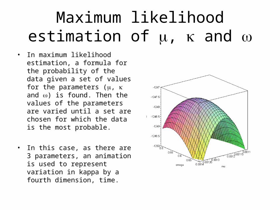
Maximum likelihood estimation of , and

• It is assumed that no more than a single mutation has occurred at each triplet since the most recent common ancestor of all sequences.

• This avoids inference of ancestral types.• And allows dimorphic segregating sites to be directly classified into

one of the four mutation types.• However, it wastes some information:

– Some triplets that are segregating cannot be classified because they involve more than a single point mutation. Rather than attempt to infer the order of mutational events, the data is ignored.

• E.g. TTG and CTA both encode Leucine, but to get from one to the other requires multiple point mutations at positions 1 and 3.

– If a triplet is segregating for more than a single codon (e.g. it is trimorphic) in the sample then ancestral type would need to be inferred. Rather than do that, the data is ignored.

• Maximum likelihood is then used to find the most probable values of , and given the observed data.


• In maximum likelihood estimation, a formula for the probability of the data given a set of values for the parameters (, and ) is found. Then the values of the parameters are varied until a set are chosen for which the data is the most probable.

• In this case, as there are 3 parameters, an animation is used to represent variation in kappa by a fourth dimension, time.


• The maximum likelihood estimates were = 0.001662 (per 2N generations) = 5.848 = 0.2598

• Therefore the rates, per codon per 2N generations were• Synonymous transversion 0.001662• Synonymous transition 0.00972• Non-synonymous transversion 0.0004318• Non-synonymous transition 0.002525

• where N is the effective population size

Underlying mutation rate, M

• Under the parameters estimated, the basic mutation rate per codon, M = 0.03819 per 2N generations, where N is the effective population size.

• Biochemical estimates of the basic mutation rate in Escherichia coli have been of the order of 5 x 10-9 per generation.

• Equating this to the true underlying mutation rate, the effective population size can be estimated as N = 1.3million.

• Such an estimate is subject to assumptions of selective neutrality, once functional constraint has been modelled as mutational bias.

• In a human pathogen such as Neisseria meningitidis, selective neutrality is highly unlikely.

E. coli rate from Drake et. al. 1998 or Drake & Holland 1999

Statistical test of hypothesis3

Statistical hypothesis testing

• This is the next stage.• First the coalescent simulations need

running.• Then we can test the MLST data for

selective neutrality.• I expect neutrality to be overwhelmingly

rejected as a null hypothesis.• Then we can go on to test the clonal

epidemic model.

Documents

Estimating evolutionary parameters for Neisseria meningitidis Based on the Czech MLST dataset