Embed Size (px)
Citation preview

Estimating Dynamic Games
Sanjog MisraAnderson UCLA
Structural Workshop 2013
Misra Estimating Dynamic Games

Estimating Dynamic Discrete Games
In this workshop we have gone through a lot.
The main topics include...
1 Foundations: Structural Models (Reiss), Causality andIdentification (Goldfarb), Instruments (Rossi), Data (Mela)
2 Methods: Static Demand Models (Sudhir), Single AgentDynamics: Theory and Econometrics (Hitsch), Static Games(Ellickson)
What you should have gleaned from their talks is that theestimation of structural models requires
Data+ Theory + Econometrics
The estimation of dynamic games combines elements from allof the above talks and requires considerable expertise inhandling data, game theory, econometrics and computationalmethods.
Misra Estimating Dynamic Games

Estimating Dynamic Discrete Games
We’ve already learned how to estimate single-agent (SA)dynamic discrete choice (DDC) models
Two main approaches
1 Full solution: NXFP (Rust, 1987)
2 Two-Step: CCP (Hotz and Miller, 1993)
In both cases, the underlying SA optimization probleminvolved agent’s solving a dynamic programming (DP)problem
With games, agent’s must solve an inter-related system of DPproblems
Their actions must be optimal given their beliefs & theirbeliefs must be correct on average (or at least self-confirming)
As you can imagine, computing equilibria can be prettycomplicated...
Misra Estimating Dynamic Games

Estimating Dynamic Discrete Games
Ericson & Pakes (ReStud, 95) and Pakes & McGuire (Rand,94) provide a framework for computing equilibria to dynamicgames.
More recently Goettler and Gordon (JPE 2012) provide analternative approach
However, using the original PM algorithm, solving areasonably complex EP-style dynamic game even once iscomputationally demanding (if not impossible)
Estimating the model using NFXP is essentially intractable
There’s also the issue of multiple equilibriaThe “incompleteness” this introduces can make it diffi cult toconstruct a proper likelihood/objective function, furthercomplicating a NFXP approach
Two-step “CCP”estimation provides a work-around thatcircumvents the iterative fixed point calculation, “solving”both problems
Misra Estimating Dynamic Games

Estimating Dynamic Discrete Games
CCP estimators were first developed by Hotz & Miller (HM,1993) & Hotz, Miller, Sanders & Smith (HMS2, 1994) forDDC modelsFour sets of authors (contemporaneously) suggested adaptingthese methods to games:1 Aguirregabiria and Mira (AM) (Ema, 2007),2 Bajari, Benkard, and Levin (BBL) (Ema, 2007),3 Pakes, Ostrovsky, and Berry (POB) (Rand, 2007), &4 Pesendorfer and Schmidt-Dengler (PSD) (ReStud, 2008),
We’ll talk about AM & BBLAM extends HM to gamesBBL extends HMS2 to games
Both are based on the framework suggested in Rust (94)More recent contributions are Blevins et al. (2012) andArcidiacono and Miller (Ema, 2011)
Misra Estimating Dynamic Games

Aguirregabiria and Mira (Ema, 2007)“Sequential Estimation of Dynamic Discrete Games”
Model
A dynamic discrete game of incomplete information.
Motivated by stylized model of retail chain competition.
Let dt be a vector of demand shifters in period t.
N firms operate in the market, indexed by i ∈ 1, 2, ...,N.In each period t, firms decide simultaneously how manyoutlets to operate - choosing from the discrete setA = 0, 1, ..., J
The decision of firm i in period t is ait ∈ AThe vector of all firms’actions is at ≡ (a1t , a2t , ..., aNt )
Misra Estimating Dynamic Games
Model
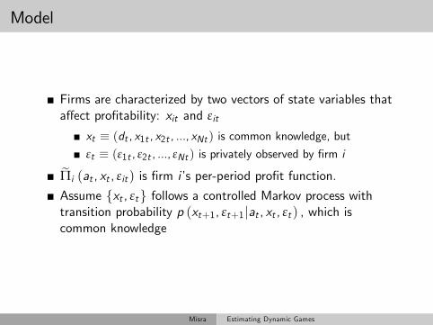
Firms are characterized by two vectors of state variables thataffect profitability: xit and εit
xt ≡ (dt , x1t , x2t , ..., xNt ) is common knowledge, butεt ≡ (ε1t , ε2t , ..., εNt ) is privately observed by firm i
Πi (at , xt , εit ) is firm i’s per-period profit function.
Assume xt , εt follows a controlled Markov process withtransition probability p (xt+1, εt+1|at , xt , εt ) , which iscommon knowledge
Misra Estimating Dynamic Games

Model
Each firm chooses its number of outlets to maximize expecteddiscounted intertemporal profits,
E ∞
∑s=t
βs−t Πi (at , xt , εit ) | xt , εit
where β ∈ (0, 1) is the (known) discount factor.The primitives of the model are the profit functions Πi (·),the transition probability p (·|·), and β
AM make the following set of assumptions...
Misra Estimating Dynamic Games

Assumptions
Misra Estimating Dynamic Games
Strategies and Bellman Equations
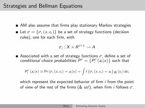
AM also assume that firms play stationary Markov strategies
Let σ = σi (x , εi ) be a set of strategy functions (decisionrules), one for each firm, with
σi : X × RJ+1 → A
Associated with a set of strategy functions σ, define a set ofconditional choice probabilities Pσ = Pσ
i (ai |x) such that
Pσi (ai |x) ≡ Pr (σi (x , εi ) = ai |x) =
∫I σi (x , εi ) = ai gi (εi ) d εi
which represent the expected behavior of firm i from the pointof view of the rest of the firms (& us!), when firm i follows σ.
Misra Estimating Dynamic Games
Expected profits
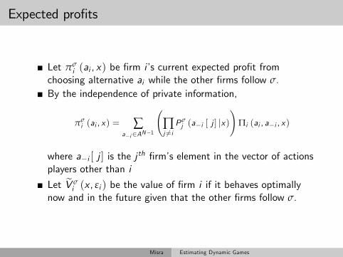
Let πσi (ai , x) be firm i’s current expected profit from
choosing alternative ai while the other firms follow σ.By the independence of private information,
πσi (ai , x) = ∑
a−i∈AN−1
(∏j 6=iPσj (a−i [ j ] |x)
)Πi (ai , a−i , x)
where a−i [ j ] is the j th firm’s element in the vector of actionsplayers other than i
Let V σi (x , εi ) be the value of firm i if it behaves optimally
now and in the future given that the other firms follow σ.
Misra Estimating Dynamic Games

Value Functions
By Bellman’s principle of optimality, we can write
V σi (x , εi ) = maxai∈A
πσi (ai , x ) + εi (ai ) + β ∑
x ′∈X
[∫V σi(x ′, ε′i
)gi(ε′i)d ε′i
]f σi(x ′ |x , ai
)(1)
where f σi (x
′|x , ai ) is the transition probability of x conditionalon firm i choosing ai and the other firms following σ:
f σi(x ′ |x , ai
)= ∑a−i∈AN−1
(∏j 6=iP σj (a−i [j ] |x )
)f(x ′ |x , ai , a−i
)
AM prefer to work with the value functions integrated overthe private information variables.
Let V σi (x) be the integrated value function∫
V σi (x , εi ) gi (dεi )
Misra Estimating Dynamic Games

Choice-Specific Value Functions
Based on this definition
V σi (x ) =
∫V σi (x , εi ) gi (d εi )
and the Bellman equation from above
V σi (x , εi ) = maxai∈A
πσi (ai , x ) + εi (ai ) + β ∑
x ′∈X
[∫V σi(x ′, ε′i
)gi(ε′i)d ε′i
]f σi(x ′ |x , ai
)(1)
we can obtain the integrated Bellman equation
V σi (x) =
∫maxai∈Avσi (ai , x) + εi (ai ) gi (d εi )
wherevσi (ai , x) ≡ πσ
i (ai , x) + β ∑x ′∈X
V σi(x ′)f σi(x ′|x , ai
)which are often referred to as choice-specific value functions.
Misra Estimating Dynamic Games

Markov Perfect Equilibria
Now it’s time to enforce the fact that σ describes equilibriumbehavior (i.e. it’s a best response)
DEFINITION: A stationary Markov perfect equilibrium (MPE)in this game is a set of strategy functions σ∗ such that for anyfirm i and any (x , εi ) ∈ X × RJ+1
σ∗i (x , εi ) = argmaxai∈A
vσ∗i (ai , x) + εi (ai )
Ultimately, an equation (somewhat) like this will be the basisof estimation
Misra Estimating Dynamic Games

Markov Perfect Equilibria
Note that πσi ,V
σi , & f
σi only depend on σ through P, so AM
switch notation to πPi ,VPi , & f
Pi so they can represent the
MPE in probability space.
Let σ∗ be a set of MPE strategies and let P∗ be theprobabilities associated with these strategies
P∗ (ai |x) =∫I ai = σ∗i (x , εi ) gi (εi ) dεi
Equilibrium probabilities are a fixed point (P∗ = Λ (P∗)),where, for any vector of probabilitiesP,Λ (P) = Λi (ai |x ;P−i ) and
Λi (ai |x ;P−i ) =∫I
(ai = arg max
ai∈A
vP∗
i (a, x) + εi (a))
gi (εi ) d εi
The functions Λi are best response probability functions
Misra Estimating Dynamic Games

Markov Perfect Equilibria
The equilibrium probabilities solve the coupled fixed-pointproblems defined by
V σi (x) =
∫maxai∈Avσi (ai , x) + εi (ai ) gi (d εi ) (2)
and
Λi (ai |x ;P−i ) =∫I
(ai = arg max
ai∈A
vP∗
i (a, x) + εi (a))
gi (εi ) d εi
(3)
Given a set of probabilities P:
The value functions V Pi are solutions of the N Bellmanequations in (2), and
Given these value functions, the best response probabilities aredefined by the RHS of (3).
Misra Estimating Dynamic Games

An Alternative Best Response Mapping
It’s easier to work with an alternative best response mapping(in probability space) that avoids the solution of the Ndynamic programming problems in (2).
The evaluation of this mapping is computationally muchsimpler than the evaluation of the mapping Λ (P), and it willprove more convenient for the estimation of the model.
Let P∗ be an equilibrium and let V P∗
1 ,V P∗
2 , ...,V P∗
N be firms’value functions associated with this equilibrium.
Misra Estimating Dynamic Games

Alternative Best Response Mapping
Because equilibrium probabilities are best responses, we canrewrite the Bellman equation
V σi (x ) =
∫maxai∈Av σi (ai , x ) + εi (ai ) gi (d εi ) (2)
as
V P∗
i (x ) = ∑ai∈A
P ∗i (ai |x )[πP
∗i (ai , x ) + e
P ∗i (ai , x )
]+ β ∑
x ′∈XV P
∗i(x ′)f P∗ (x ′ |x
)(4)
where f P∗(x ′|x) is the transition probability of x induced by
P∗
eP∗
i (ai , x) is the expectation of εi (ai ) conditional on x andon alternative ai being optimal for player i
Misra Estimating Dynamic Games
Alternative Best Response Mapping
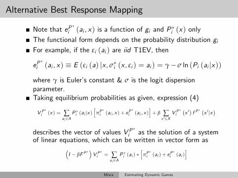
Note that eP∗
i (ai , x) is a function of gi and P∗i (x) only
The functional form depends on the probability distribution giFor example, if the εi (ai ) are iid T1EV, then
eP∗
i (ai , x) ≡ E (εi (a) |x , σ∗i (x , εi ) = ai ) = γ−σ ln (Pi (ai |x))
where γ is Euler’s constant & σ is the logit dispersionparameter.Taking equilibrium probabilities as given, expression (4)
V P∗
i (x ) = ∑ai∈A
P ∗i (ai |x )[πP
∗i (ai , x ) + e
P ∗i (ai , x )
]+ β ∑
x ′∈XV P
∗i(x ′)f P∗ (x ′ |x
)
describes the vector of values V P∗
i as the solution of a systemof linear equations, which can be written in vector form as(
I − βF P∗)V P
∗i = ∑
ai∈AP ∗i (ai ) ∗
[πP
∗i (ai ) + e
P ∗i (ai )
]
Misra Estimating Dynamic Games

Alternative Best Response Mapping
Let Γi (P∗) ≡ Γi (x ;P∗) : x ∈ X be the solution to thissystem of linear equations, such that V P
∗i (x) = Γi (x ;P∗) .
For arbitrary probabilities P, the mapping
Γi (P ) =(I − βF P
∗)−1 ∑ai∈A
P ∗i (ai ) ∗[πP
∗i (ai ) + e
P ∗i (ai )
](5)
can be interpreted as a valuation operator.An MPE is then a fixed point Ψ (P) ≡ Ψi (ai |x ;P) where
Ψi (ai |x ;P ) =∫I
(ai = arg max
ai ∈A
πPi (a, x ) + εi (a) + β ∑
x ′∈XΓi(x ′;P
)f Pi(x ′ |x , a
))gi (εi ) d εi
(6)
By definition, an equilibrium vector P∗ is a fixed point of Ψ.AM’s Representation Lemma establishes that the reverse isalso true.
Equation (6) will be the basis of estimation
Misra Estimating Dynamic Games

Estimation
Assume the researcher observes M geographically separatemarkets over T periods, where M is large and T is small.
The primitives Πi , gi , f , β : i ∈ I are known to theresearcher up to a finite vector of structural parametersθ ∈ Θ ⊂ R |Θ|.
β is assumed known (it’s very diffi cult to estimate)
We now incorporate θ as an explicit argument in theequilibrium mapping Ψ.Let θ0 ∈ Θ be the true value of θ in the population
Under Assumption 2 (i.e., conditional independence), thetransition probability function f can be estimated fromtransition data using a standard maximum likelihood methodand without solving the model.
Misra Estimating Dynamic Games

Assumptions on DGP
Misra Estimating Dynamic Games

Maximum Likelihood Estimation
Define the pseudo likelihood function
QM (θ,P) =1M
M
∑m=1
T
∑t=1
N
∑i=1lnΨi (aimt |xmt ;P, θ)
where P is an arbitrary vector of players’choice probabilities.
Consider first the hypothetical case of a model with a uniqueequilibrium for each possible value of θ ∈ Θ.Then the maximum likelihood estimator (MLE) of θ0 can bedefined from the constrained multinomial likelihood
θMLE = argmaxθ∈Θ
QM (θ,P) subject to P = Ψ (θ,P)
Misra Estimating Dynamic Games

MLE
However, with multiple equilibria the restriction P = Ψ (θ,P)does not define a unique vector P, but a set of vectors.In this case, the MLE can be defined as
θMLE = arg maxθ∈Θ
supP∈(0,1)N |X |
QM (θ,P) subject to P = Ψ (θ,P)
Thus, for each candidate θ, we need to compute all thevectors P that constitute equilibria (given θ) and select theone with the highest value of QM (θ,P) .
At present, there are no known methods that can do so(robustly).
Therefore, AM introduce a class of pseudo maximumlikelihood estimators.
Misra Estimating Dynamic Games

Pseudo Maximum Likelihood (PML) Estimation
The PML estimators try to minimize the number ofevaluations of Ψ for different vectors of players’probabilitiesP.
Suppose that we know the population probabilities P0 andconsider the (infeasible) PML estimator
θ = argmaxθ∈Θ
QM(θ,P0
)Under standard regularity conditions, this estimator is√M-CAN, but infeasible since P0 is unknown.
However, if we can obtain a√M-consistent nonparametric
estimator of P0, then we can define the feasible two-step PMLestimator
θ2S = argmaxθ∈Θ
QM(θ, P0
)Misra Estimating Dynamic Games

PML
√M-CAN of P0 (+ regularity conditions) are suffi cient to
guarantee that the PML estimator is√M-CAN.
There are two good reasons to care about this estimator
1 It deals with the indeterminacy problem associated withmultiple equilibria (it’s robust)
2 Furthermore, repeated solutions of the dynamic game areavoided, which can result in significant computational gains(it’s simple)
Misra Estimating Dynamic Games

PML: Drawbacks
However, the two-step PML has some drawbacks
1 Its asymptotic variance depends on the variance Σ of thenonparametric estimator P0.
Therefore, it can be very ineffi cient when Σ is large.
2 For the sample sizes available in actual applications, thenonparametric estimator of P0 can be very imprecise (smallsample bias).
There’s a curse of dimensionality here...
3 For some models, it’s impossible to obtain consistentnonparametric estimates of P0.
e.g. models with unobserved market characteristics.
To address these issues, AM introduce the Nested PseudoLikelihood estimator.
Misra Estimating Dynamic Games

Nested Pseudo Likelihood (NPL) Method
NPL is a recursive extension of the two-step PML estimator.
Let P0 be a (possibly inconsistent) initial guess of the vectorof players’choice probabilities.
Given P0, the NPL algorithm generates a sequence ofestimators
θK : K ≥ 1
, where the K-stage estimator is
defined asθK = argmax
θ∈ΘQM
(θ, PK−1
)and the probabilities
PK : K ≥ 1
are obtained recursively as
PK = Ψ(θK , PK−1
)
Misra Estimating Dynamic Games

NPL
If the initial guess P0 is a consistent estimator, all elements ofthe sequence of estimators
θK : K ≥ 1
are consistent
However, AM are interested in the properties of the estimatorin the limit (if it converges)
If the sequence
θK , PKconverges, its limit
(θ, P
)is such
thatθ maximizes QM
(θ, P
)and P = Ψ
(θ, P
)and any pair that does so is a NPL fixed point.
AM show that a NPL fixed point always exists and, if there ismore than one, the one with the highest value of the pseudolikelihood is a consistent estimator
Of course, it may be very diffi cult to find multiple roots
Misra Estimating Dynamic Games

NPL
NPL preserves the two main advantages of PML
1 It’s feasible in models with multiple equilibria, and
2 It minimizes the number of evaluations of the mapping Ψ fordifferent values of P
Furthermore
1 It’s more effi cient than either infeasible or two-step PML(because it imposes the MPE condition in sample)
2 It reduces the finite sample bias generated by impreciseestimates of P0
3 It doesn’t require initially consistent P0’s (so it canaccommodate unobserved heterogeneity)
AM show how to extend NPL to settings with permanentunobserved heterogeneity, but let’s skip that & look at someMonte Carlos
Misra Estimating Dynamic Games

Monte Carlos
Consider a simple entry/exit example where 5 firms canoperate at most 1 store, so ait ∈ 0, 1Variable profit is given by
θRS ln (Smt )− θRN ln(1+∑j 6=i ajmt
)where Smt is the size of market m in period t, and θRS & θRNare parameters to be estimatedThe profit function of an active firm is
Πimt (1) = θRS ln (Smt )− θRN ln(1+∑j 6=i ajmt
)− θFC ,i − θEC (1− aim,t−1)+ εimt
where θFC ,i is fixed cost, θEC is entry cost, and εimt ∼ T1EVThe profit function of an inactive firm is simply
Πimt (0) = εimt
Misra Estimating Dynamic Games

Monte Carlos
ln (Smt ) follows a discrete first order Markov process, withknown transition matrix and finite support 1, 2, 3, 4, 5Fixed operating costs are
θFC ,1 = −1.9, θFC ,2 = −1.8, θFC ,3 = −1.7, θFC ,4 = −1.6, θFC ,5 = −1.5
so that firm 5 is most effi cient and firm 1 is least effi cient.
θRS = 1 and β = .95 throughout, but AM will vary θRN andθEC
Misra Estimating Dynamic Games

Monte Carlos
The space of common knowledge state variables (Smt , at−1)has 25 × 5 = 160 cells.There’s a different vector of CCPs for each firm, so thedimension of the CCP vector for all firms is 5× 160 = 800.For each experiment, they compute a MPE.
The equilibrium is obtained by iterating the best responseprobability mapping starting with a 800× 1 vector of choiceprobabilities (guesses) - (e.g. Pi (ai = 1|x) = .5 ∀x , i)They can then calculate the steady state distribution andgenerate fake data.
Table II presents some descriptive statistics associated withthe MPE of each experiment.
Misra Estimating Dynamic Games

Markov Perfect Equilibria for each experiment
Misra Estimating Dynamic Games

Monte Carlos
They then calculate the two-step PML and NPL estimatorsusing the following choices for the initial vector of probabilities
1 The true vector of equilibrium probabilities P0
2 Nonparametric frequency estimates
3 Logits (for each firm) with the log of market size andindicators of incumbency status for all firms as explanatoryvariables, and
4 Independent random draws from a U(0, 1) r.v.
Tables IV and V summarize the results
Misra Estimating Dynamic Games

Monte Carlo Results
Misra Estimating Dynamic Games

Monte Carlo Results
Misra Estimating Dynamic Games

Discussion of Results
The NPL algorithm always converged to the same estimates(regardless of the value of P0)
The algorithm converged faster when initialized with logitestimates
The 2S-Freq estimator is highly biased in all experiments,although its variance is sometimes smaller than the NPL and2S-True estimators.
It’s main drawback is small sample bias...
The NPL estimator performs very well relative to the 2S-Trueboth in terms of variance and bias.
In all the experiments, the most important gains associatedwith the NPL estimator occur for the entry cost parameter.
Misra Estimating Dynamic Games

Motivation for BBL
A big drawback of the AM approach (and PSD & POB aswell) is that it’s designed for discrete controls (and discretestates)
A big selling point of BBL is that it can
However,
1 It’s not completely clear that AM can’t be extended tocontinuous controls and states (see, e.g., Arcidiacono andMiller (2011))
2 The way BBL “handles” continuous controls is probablyinfeasible (unless there are no structural shocks to investment)
3 BBL’s objective function can be diffi cult to optimize, so youmight want to mix & match a bit.
Let’s look now at how BBL works...
Misra Estimating Dynamic Games

Background for BBL (HMSS)
The original idea for the methods proposed in BBL came fromHotz, Miller, Sanders and Smith (1994)
They proposed a two-step (really 3) approach
1 Estimate the transition kernels f (s ′|s, a) and CCPs P (a|s)from the data
2 Approximate V(s |P)using Monte-Carlo approaches
3 Construct and maximize an objective function to obtainparameters
Let’s look how this might work...
Misra Estimating Dynamic Games
Forward Simulation (HMSS)
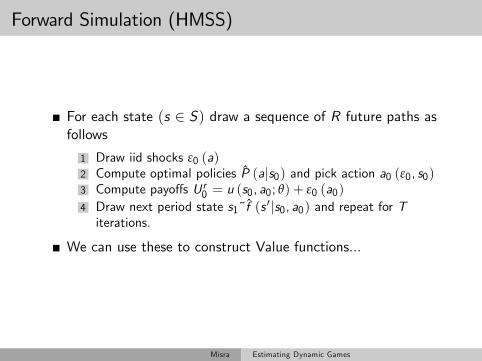
For each state (s ∈ S) draw a sequence of R future paths asfollows
1 Draw iid shocks ε0 (a)2 Compute optimal policies P (a|s0) and pick action a0 (ε0, s0)3 Compute payoffs Ur0 = u (s0, a0; θ) + ε0 (a0)4 Draw next period state s1˜f (s ′|s0, a0) and repeat for Titerations.
We can use these to construct Value functions...
Misra Estimating Dynamic Games

Value Function (HMSS)
At some T we stop the forward simulation and use the factthat
V r (s0) =T
∑t=0
βtU rt
To construct
V(s0|P
)=1R
R
∑r=1
V r (s0)
We can then obtain an estimator usingA Pseudo Likelihood, GMM or Least Squares
maxθ
∑t
∑iait lnΨ
(ait |sit , V
)min
θ∑i
(∑t
(ait −Ψ
(ait |sit , V
)Zit))
Ω−1(
∑t
(ait −Ψ
(ait |sit , V
)Zit))′
minθ
(P (a|s)−Ψ
(a|s, V
))′W−1
(P (a|s)−Ψ
(a|s, V
))Misra Estimating Dynamic Games

Bajari, Benkard, and Levin (Ema, 2007)Estimating Dynamic Models of Imperfect Competition
So what does BBL do?
Extends HMSS to gamesGeneralizes the idea to continuous actionsProposes an inequality conditions for estimation (Boundsestimator)
The key element of BBL is that it (like AM 2007) allows theresearch to be agnostic about equilibrium selection
and side-step the multiple equilibria problem.
Misra Estimating Dynamic Games

Bajari, Benkard, and Levin (Ema, 2007)Estimating Dynamic Models of Imperfect Competition
Notation
The game is in discrete time with an infinite horizon
There are N firms, denoted i = 1, ...,N making decisions attimes t = 1, 2, ...,∞Conditions at time t are summarized by discrete statesst ∈ S ⊂ RL
Given st , firms choose actions simultaneouslyLet ait ∈ Ai denote firm i’s action at time t, andat = (a1t , ..., aNt ) the vector of time t actions
Misra Estimating Dynamic Games

Notation
Before choosing its action, each firm i receives a private shockνit drawn iid from Gi (·|st ) with support Vi ⊂ RM
Denote the vector of private shocks νt = (ν1t , ..., νNt )
Firm i’s profits are given by πi (at , st , νit ) and firms share acommon (& known) discount factor β < 1
Given st , firm i’s expected profit (prior to seeing νit) is
E
[∞
∑τ=t
βτ−tπi (aτ, sτ, νiτ)|st
]
where the expectation is over current shocks and actions, aswell as future states, actions, and shocks.
Misra Estimating Dynamic Games

State Transitions & Equilibrium
st+1 is drawn from a probability distribution P (st+1|at , st )They focus on pure strategy MPE
A Markov strategy is a function σi : S × Vi → AiA profile of Markov strategies is a vector, σ = (σ1, ..., σN ) ,where σ : S × V1 × ...× VN → A
Given σ, firm i’s expected profit can then be writtenrecursively
Vi (s; σ) = Eν
[πi (σ (s, ν) , s, νi ) + β
∫V(s′; σ
)dP(s′|σ (s, ν) , s
)|s]
The profile σ is a MPE if, given opponent profile σ−i , eachfirm i prefers strategy σi to all other alternatives σ′i
Vi (s; σ) ≥ Vi(s; σ′i , σ−i
)Misra Estimating Dynamic Games

Structural Parameters
The structural parameters of the model are the discount factorβ, the profit functions π1, ...,πN , the transition probabilitiesP, and the distributions of private shocks G1, ...,GN .
Like AM, they treat β as known and estimate P directly fromthe observed state transitions.
They assume the profits and shock distributions are knownfunctions of a parameter vector θ : πi (a, s, νi ; θ) andGi (νi |s, θ) .The goal is to recover the true θ under the assumption thatthe data are generated by a MPE.
Misra Estimating Dynamic Games

Example: Dynamic Oligopoly
Their main (novel) example is based on the EP framework.
Incumbent firms are heterogeneous, each described by itsstate zit ∈ 1, 2, ..., z ; potential entrants have zit = 0Incumbents can make an investment Iit ≥ 0 to improve theirstate
An incumbent firm i in period t earns
qit (pit −mc (qit , st ; µ))− C (Iit , νit ; ξ)
where pit is firm i’s price, qit = qi (st ,pt ;λ) is quantity,mc (·) is marginal cost, and νit is a shock to the cost ofinvestment.
C (Iit , νit ; ξ) is the cost of investment.
Misra Estimating Dynamic Games

Example: Dynamic Oligopoly
Competition is assumed to be static Nash in prices.
Firms can also enter and exit.
Exitors receive φ and entrants pay νet , an iid draw from GeIn equilibrium, incumbents make investment and exit decisionsto maximize expected profits.
Each incumbent i uses an investment strategy Ii (s, νi ) andexit strategy χi (s, νi ) chosen to maximize expected profits.Entrants follow a strategy χe (s, νe ) that calls for them toenter if the expected profit from doing so exceeds its entrycost.
Misra Estimating Dynamic Games

First Stage Estimation
The goal of the first stage is to estimate the state transitionprobabilities P(s′|a, s) and equilibrium policy functions σ(s, ν)The second stage will use the equilibrium conditions fromabove to estimate the structural parameters θ
In order to obtain consistent first stage estimates, they mustassume that the data are generated by a single MPE profile σ
This assumption has a lot of bite if the data come frommultiple markets
It’s quite weak if the data come from only a single market
Misra Estimating Dynamic Games

First Stage Estimation
Stage “0”:
The static payoff function will typically be estimated “off line”in a 0th stage (e.g. BLP, Olley-Pakes)
Stage 1:
It’s usually fairly straightforward to run the first stage: just“regress”actions on states in a “flexible manner”.Since these are not structural objects, you should be as flexibleas possible. Why?Of course, if s is big, you may have to be very parametric here(i.e. OLS regressions and probits).
In this case, your second stage estimates will be inconsistent...
Continuous actions are especially tricky (hard to benonparametric here)
Misra Estimating Dynamic Games

Estimating the Value Functions
After estimating policy functions, firm’s value functions areestimated by forward simulation.
Let Vi (s, σ; θ) denote the value function of firm i at state sassuming firm i follows the Markov strategy σi and rival firmsfollow σ−i
Then
Vi (s, σ; θ) = E
[∞
∑0=t
βtπi (σ (st , νt ) , st , νit ; θ)|s0 = s; θ]
where the expectation is over current and future values of stand νt
Given a first-stage estimate P of the transition probabilities,we can simulate the value function Vi (s, σ; θ) for any strategyprofile σ and parameter vector θ.
Misra Estimating Dynamic Games

Estimating the Value Functions
A single simulated path of play can be obtained as follows:
1 Starting at state s0 = s, draw private shocks νi0 fromGi (·|s0, θ) for each firm i .
2 Calculate the specified action ai0 = σi (s0, νi0) for each firm i ,and the resulting profits πi (a0, s0, νi0; θ)
3 Draw a new state s1 using the estimated transitionprobabilities P (·|a0, s0)
4 Repeat steps 1-3 for T periods or until each firm reaches aterminal state with known payoff (e.g. exits from the market)
Averaging firm i’s discounted sum of profits over many pathsyields an estimate Vi (s, σ; θ) , which can be obtained for any(σ, θ) pair, including both the “true”profile (which youestimated in the first stage) and any alternative you care toconstruct.
Misra Estimating Dynamic Games
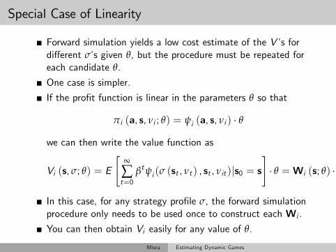
Special Case of Linearity
Forward simulation yields a low cost estimate of the V’s fordifferent σ’s given θ, but the procedure must be repeated foreach candidate θ.
One case is simpler.
If the profit function is linear in the parameters θ so that
πi (a, s, νi ; θ) = ψi (a, s, νi ) · θ
we can then write the value function as
Vi (s, σ; θ) = E
[∞
∑t=0
βtψi (σ (st , νt ) , st , νit )|s0 = s]· θ =Wi (s; θ) · θ
In this case, for any strategy profile σ, the forward simulationprocedure only needs to be used once to construct each Wi .
You can then obtain Vi easily for any value of θ.
Misra Estimating Dynamic Games

Second Stage Estimation
The first stage yields estimates of the policy functions, statetransitions, and value functions.
The second stage uses the model’s equilibrium conditions
Vi (s; σi , σ−i ; θ) ≥ Vi(s; σ′i , σ−i ; θ
)to recover the parameters θ that rationalize the strategyprofile σ observed in the data.
They show how to do so for both set and point identifiedmodels
We will focus on the point identified case here.
Misra Estimating Dynamic Games

Second Stage Estimation
To see how the second stage works, define
g (x ; θ, α) = Vi (s; σi , σ−i ; θ, α)− Vi(s; σ′i , σ−i ; θ, α
)where x ∈ X indexes the equilibrium conditions and αrepresents the first-stage parameter vector.
The inequality defined by x is satisfied at θ, α if g (x ; θ, α) ≥ 0Define the function
Q (θ, α) ≡∫(min g (x ; θ, α) , 0)2 dH(x)
where H is a distribution over the set X of inequalities.
Misra Estimating Dynamic Games

Second Stage Estimation
The true parameter vector θ0 satisfies
Q (θ0, α0) = 0 = minθ∈Θ
Q(θ, α0)
so we can estimate θ by minimizing the sample analog ofQ(θ, α0)
The most straightforward way to do this is to draw firms andstates at random and consider alternative policies σ′i that areslight perturbations of the estimated policies.
Misra Estimating Dynamic Games

Second Stage Estimation
We can then use the above forward simulation procedure toconstruct analogues of each of the Vi terms and construct
Q (θ, α) ≡ 1nI
nI
∑k=1
(min g (Xk ; θ, α) , 0)2
How? By drawing nI different alternative policies, computingtheir values, finding the difference versus the optimal policypayoff, and using an MD procedure to estimate theparameters that minimize these profitable deviations.
Their estimator minimizes the objective function at α = αn
θ = argminθ∈Θ
Qn (θ, αn)
See the paper for the technical details.
Misra Estimating Dynamic Games

Example: Dynamic Oligopoly
Let’s see how they estimate the EP model.
First, they have to choose some parameterizations.
They assume a logit demand system for the product market.
There are M consumers with consumer r deriving utility Urifrom good i
Uri = γ0 ln(zi ) + γ1 ln (yr − pi ) + εri
where zi is the quality of firm i , pi is firm i’s price, yr isincome, and εri is an iid logit error
All firms have identical constant marginal costs of production
mc(qi ; µ) = µ
Misra Estimating Dynamic Games

Example: Dynamic Oligopoly
Each period, firms choose investment levels Iit ∈ R+ toincrease their quality in the next period.
Firm i’s investment is successful with probability
ρIit(1+ ρIit )
in which case quality increases by one, otherwise it doesn’tchange.
There is also an outside good, whose quality moves up by onewith probability δ each period.
Firm i’s cost of investment is
C (Ii ) = ξ · Ii
so there is no shock to investment (it’s deterministic)
Misra Estimating Dynamic Games

Example: Dynamic Oligopoly
The scrap value φ is constant and equal for all firms.
Each period, the potential entrant draws a private entry costνet from a uniform distribution on
[νL, νH
]The state variable st = (Nt , z1t , ..., zNt , zout ,t ) includes thenumber of incumbent firms and current product qualities.
The model parameters are γ0,γ1, µ, ξ, φ, νL, νH , ρ, δ, β, & y
They assume that β & y are known, ρ & δ are transitionparameters estimated in a first stage, γ0,γ1, & µ are demandparameters (also estimated in a first stage), so the main(dynamic) parameters are simply θ =
(ξ, φ, νL, νH
)Due to the computational burden of the PM algorithm, theyconsider a setting in which only ≤ 3 firms can be active.They generated datasets of length 100-400 periods using PM.
Misra Estimating Dynamic Games

Example: Dynamic Oligopoly
Here are the parameters they use.
Misra Estimating Dynamic Games

Example: Dynamic Oligopoly
The first stage requires estimation of the state transitions andpolicy functions (as well as the demand and mc parameters).
For the state transitions, they used the observed investmentlevels and qualities to estimate ρ and δ by MLE.
They estimated the demand parameters by MLE as well, usingquantity, price, and quality data.
They recover µ from the static mark-up formula.
They used local linear regressions with a normal kernel toestimate the investment, entry, and exit policies.
Misra Estimating Dynamic Games

Example: Dynamic Oligopoly
Given strategy profile σ = (I ,χ,χe ), the incumbent valuefunction is
Vi (s; σ) = W 1 (s; σ) +W 2 (s; σ) · ξ +W 3 (s; σ) · φ
= E
[∞
∑t=0
βt πi (st )|s = s0
]− E
[∞
∑t=0
βt Ii (st )|s = s0
]· ξ
+E
[∞
∑t=0
βtχi (st )|s = s0
]· φ
where the first term πi (st ) is the static profit of incumbent igiven state stThe 2nd term is the expected PV of investment
The 3rd term is the expected PV of the scrap value earnedupon exit.
Misra Estimating Dynamic Games

Example: Dynamic Oligopoly
To apply the MD estimator, they constructed alternativeinvestment and exit policies by drawing a mean zero normalerror and adding it to the estimated first stage investment andexit policies.
They used ns = 2000 simulation paths, each having length atmost 80, to compute the PV W 1,W 2,W 3 terms for thesealternative policies.
They can then estimate ξ & φ using their MD procedure.
It’s also straightforward to estimate the entry cost distribution(parametrically or non-parametrically) - see the paper fordetails.
Misra Estimating Dynamic Games

Example: Dynamic Oligopoly
Truth: ξ = 1 & φ = 6
For small sample sizes, there is a slight bias in the estimatesof the exit value.
Investment cost parameters are spot on.
Misra Estimating Dynamic Games

Example: Dynamic Oligopoly
Truth: ξ = 1, φ = 6, νl = 7, & νh = 11
The subsampled standard errors are on average slightlysmaller than the true SEs.
This is likely due to small sample sizes.
Misra Estimating Dynamic Games
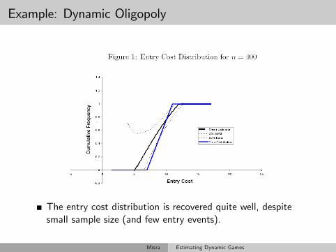
Example: Dynamic Oligopoly
The entry cost distribution is recovered quite well, despitesmall sample size (and few entry events).
Misra Estimating Dynamic Games

Conclusions
Both AM & BBL are based on the same underlying idea (CCPestimation)
As such, it’s quite possible to mix and match from the twoapproaches
e.g. forward simulate the CV terms and use a MNL likelihood
We have found AM-style approaches easier to implement, butthat might be idiosyncratic.
Applications in marketing are growing: Goettler and Gordon(2012), Ellickson, Misra, Nair (2012), Misra and Nair (2011),Chung et al. (2012) ...
If you are interested in applying this stuff, you should readeverything you can get your hands on!
Misra Estimating Dynamic Games