Embed Size (px)
Citation preview
Estimating Disaggregate Production Functions: An Application to Northern Mexico
by Richard E Howitt* and Siwa Msangi**
July 2006
* Department of Agricultural and Resource Economics, University of California, Davis, California, 95616 email [email protected]. ** Post Doctoral Fellow, International Food Policy Research Institute, Washington, DC. Email [email protected] authors gratefully acknowledge the cooperation of Musa Asad and Ariel Dinar at the World Bank.
Introduction
This paper develops a method to estimate disaggregated production function
models from minimal data sets. Disaggregated models enable the distributional
effects of policies to be measured across farm size or location. In addition if, as is
common, there is heterogeneity in the sample, spatial differences in policy impacts
and input use are also important. Also, with a heterogeneous sample, a disaggregated
set of models may predict policy response by farmers more accurately, where
aggregation bias exceeds the small sample error in disaggregated models. Throughout
the paper, we assume that the sample size is fixed, and strive to maximize the policy
information from it. The central question facing an empirical researcher is what level
of disaggregation makes the best use of the data set for the purpose in hand. The
purpose that we focus on is the prediction of policy impacts on farmers in terms of
their net income, and use of natural resources in farm production.
A primal approach to production functions has several attractive properties for
production models subject to fixed factor constraints. An important characteristic of
primary farm survey data is the frequent occurrence of incomplete factor prices due
subsidized inputs, family labor, and government regulation. This absence of market
prices for family labor, water, and often land makes the traditional dual approach
inoperable. In addition, when surveyed, farmers may recall data on primal variables
more accurately than the corresponding dual data. Finally, primal production models
are able to directly interact with more detailed models of physical processes.
Despite the very small sample size, the use of maximum entropy estimators
(GME) enables us to estimate all the model parameters, and three measures of model
fit, R2, percent absolute deviation, and normalized entropy. Since we are interested in
models that can address policy questions, the emphasis in this paper is on the ability
2
of the model to reproduce the existing production system and predict the
disaggregated outcomes of policy changes.
In many developed and developing agricultural economies there is considerable
emphasis on the effect of agricultural policies and production on the environment, and
conversely, the effect of environmental policies on the agricultural sector. This
emphasis may rekindle interest in the use of production function models for many
policy problems. There are several reasons why production functions are suited to the
analysis of agricultural- environmental policy. First, environmental values are
measured in terms of the physical outcomes of agricultural activity. Second, some
environmental policies are formulated as constraints on input use. Third, economic
models of agricultural and environmental policy impacts often have to formally
interact with process models of the physical systems. Such models require the
economic output in terms of primal values.
Several authors have emphasized the need to spatially disaggregate models for
environmental policy analysis (Antle & Capalbo, 2001; Just & Antle, 1990).
However, such disaggregation is often made difficult either by the limited availability
of disaggregate data or, if such data is present, the lack of enough degrees of freedom
to identify disaggregate parameters within a classical estimation framework.
Generalized Maximum Entropy (GME) estimation techniques (Golan et al., 1996(a))
have come into increasing use by researchers who seek to achieve higher levels of
disaggregation in the face of these data problems (Lence & Miller, 1998; Lansink et
al., 2001; Golan et al., 1994, 1996(b)). Given the inherent heterogeneity of soils and
other agricultural resources, aggregating across heterogeneous regions leads to
aggregation bias. Conversely, ill-conditioned or ill-posed GME estimates may be less
precise due to the small sample on which they are based. An additional advantage that
3
speaks in favor of maximum entropy based alternatives is the ability to formally
incorporate additional data or informative priors into the estimation process, in a
Bayesian fashion.
Substitution activity at the intensive and extensive margins is a key focus of
agricultural-environmental policy analysis. A basic policy approach is to provide
incentives or penalties that lead to input substitution under a given agricultural
technology. Such substitutions at the intensive margin can reduce the environmental
cost of producing traditional agricultural products or that of jointly producing
agricultural and environmental benefits. These policies cannot be evaluated without
explicit representation of the agricultural production process. It follows, therefore, that
the potential for substitution should be explicitly modeled within a multi-input multi-
output production framework.
The disaggregated multi-input, multi-output CES model in this paper has the
ability to model at all three margins that represent farmer response to changed prices,
costs or resource availability. The same approach has been applied to other flexible
functional forms, such as, quadratic, square root, generalized Leontieff and trans-log
specifications.
This combination of methodology distinguishes our approach with other GME
production analyses using in the literature (Zhang & Fan, 2001; Lence & Miller,
1998). The GME estimates given in this paper do, however, converge to consistent
estimates when the sample size is increased and have been shown to have the same
asymptotic properties as conventional likelihood estimators (Mittlehammer et al.,
2000).
GME estimators require the definition of support values for each parameter that
are implicit bounded priors on the parameters. Several authors have shown that
4
support values specification can have a strong influence on the resulting estimates. In
addition, if the support values are specified in an “ad hoc” manner it is possible that
there is no feasible solution to the resulting GME estimation problem. We use values
from a calibrated optimization model to ensure that the supports are centered on
values that are a feasible solution to the data constraints, and consistent with prior
parameter values. Given the support values, we estimate the production function
parameters, input shadow values, and returns to scale in a simultaneous GME
specification.
This specification of support values differentiates our approach with other GME
production analyses using in the literature (Zhang & Fan, 2001; Lence & Miller,
1998), in fact, the empirical GME literature says very little about how a set of feasible
and consistent support values are defined for several interdependent parameters. We
differ from Heckelei and Wolff (2003) by using calibrated optimization models to
define the prior sets of support values, but, like Heckelei and Wolff, we estimate
production function parameters, and factor input shadow values, in a simultaneous
GME specification.
In addition, we generate the finite sample distribution properties of the resulting
GME estimates by bootstrapping the procedure (Efron & Tibsharani, 1993). To our
knowledge, this is the first time that the bootstrap method has been used to obtain
parameter distributions for GME estimators. Previous work has tested GME results
for sensitivity to their support spaces, or has used Monte Carlo results to approximate
asymptotic parameter distributions. However, since our aim is to use small data
samples, bootstrapping seems a natural method to generate the finite sample
properties, and can be simply implemented.
5
The ability to simulate policy alternatives reliably with constrained profit
maximization requires a model that satisfies the marginal and total product conditions
and has stability in the second order profit maximizing conditions. It is our belief that
those who use policy models are more interested in reproducing observed behavior
and simulating beyond the base scenario, than in testing for the curvature properties of
the underlying production function. Within our simulation framework, we can also
impose policy restrictions in the form of constraints on the estimated farm production
model.
Section II of the paper briefly reviews modeling methods used to estimate the
effect on land use of agricultural and environmental policies. Section III develops the
production model estimation and bootstrap procedure within the GME framework.
Section IV contains an empirical application to a data set from a primary survey of 27
farms in the Rio Bravo region of Northern Mexico. The randomly selected farm
sample contains a very wide range of farm size. The central point is whether the
production parameters of different farm sizes vary sufficiently to make disaggregated
models, better estimates of policy response than estimates based on the whole sample.
Essentially we are testing whether disaggregated policy models are better predictors
of farmer behavior despite the minimal data sets used by the GME estimators.
Conclusions are drawn in Section V
II. Methods for Modeling Disaggregated Agricultural Production.
6
The approach that we use in this paper addresses the shortcomings of
representative farmer models enumerated by Antle & Capalbo (2001), when they cite
the limited range of response in the typical representative farm model. The
disaggregated production models capture the individual heterogeneity of the local
production environment, whether it is in terms of land quality or farm-size specific
effects, and allows the estimated production functions to replicate the differences in
input usage and outputs.
Love (1999) made the point that the level of disaggregation matters in terms of the
degree of firm-level heterogeneity and other localized idiosyncrasies that get averaged
out of the sample. This affects the likelihood of observing positive results for tests of
neo-classical behavior, such as cost minimization or profit maximization. In our
approach, we impose curvature conditions on the estimated production function, since
we are aiming for models that reproduce behavior rather than test for it. The relative
stability we observe within cropping systems, despite the presence of substantial yield
and price fluctuations is informal empirical evidence that farmers act as if their profit
functions are convex in crop allocation. The gradual adjustment of agricultural
systems to changes in relative crop profitability suggests that farmers adjust by
progressive changes over time, along all the margins of substitution, rather than going
from one corner solution to the next.
Zhang & Fan (2001) conclude that the behavioral assumptions of profit
maximization are too strong for the example to which they applied a GME production
function estimation. While their level of aggregation was severe, they made the case
for using GME on the basis of its ability to incorporate non-sample information and to
deal with imperfectly observed activity-specific inputs. Within our framework, we are
able to implement more flexible functional forms for production than that used by
7
Zhang & Fan, as well as avoid imposing constant returns to scale, as a result of our
higher level of disaggregation.
Just et al (1983), stated in their classic production paper that their:
“Methodology is based on the following assumptions that seem to characterize
most agricultural production:
(a)Allocated inputs. Most agricultural inputs are allocated by farmers to
specific production activities..
(b)Physical constraints. Physical constraints limit the total quantity of some
inputs that a farmer can use in a given period of time …
(c) Output determination. Output combinations are determined uniquely by the
allocation of inputs to various production activities aside from random,
uncontrollable forces.”
Just et al’s specification admits jointness in multioutput production only
through the common restrictions on allocatable inputs. The specification in this paper
has constraints on the land available, but also allows for jointness between crops in a
region as reflected by the deviations of crop value marginal products from the
opportunity cost of restricted land inputs.
The current range of approaches to agricultural production modeling and the
associated analysis of environmental impacts, seems to fall into three groups, namely,
disaggregated calibrated or constrained programming models (McCarl, 2000 ; Alig et
al., 1998; CVPM1, 1997; CAPRI2, 2000) disaggregated logistic land use models (Wu
& Babcock, 1999) and A, and aggregate econometric land use models (Mendelsohn et
al., 1994 ). Antle and Valdivia (2006)
1 Central Valley Production Model , used in the 1997 Programmatic Environmental Impact Statement of the Central Valley Project Improvement Act (see references). 2 Common Agricultural Policy Regional Impact (http://www.agp.uni-bonn.de/agpo/rsrch/capri/)
8

III Using Generalized Maximum Entropy to Estimate Production Functions The nature of the data set defines the estimation method to be used. For
disaggregated policy models, the available data usually takes the form of a cross-
sectional survey sample taken over each disaggregated region. A reassuring
characteristic of generalized maximum entropy (GME) estimators is that while they
can estimate consistent parameter values from ill-conditioned or ill-posed problems,
their large sample estimates enjoy the usual classical properties (Mittlehammer et al,
2000). The GME estimation approach advanced in this paper is completely in accord
with classical econometric estimators for large sample problems and uses a standard
bootstrap approach to estimate GME parameter distributions. The novelty of the paper
lies in the idea that the modeler does not have to accept the stricture of conventional
degrees of freedom, but may specify a complex model at the level of disaggregation
that is thought to minimize the effect of estimation errors and aggregation bias on the
model outcome. The modeler can specify flexible multi-input production functions for
any number of observations and calibrate closely to the base conditions. Essentially
we show that a minimal level of data that would, in the past, have restricted the
modeler to a simple linear programming model, can now be calibrated and
reconstructed as a set of multi-input CES production functions.
The first order conditions for optimal allocation have to incorporate the
shadow value of any constraints on inputs. Since the allocatable inputs are restricted
in quantity, and rotational interdependencies can exist between crops, we use a
modified PMP model ( Howitt 1995) on each data sample to obtain a numerical value
for a prior value for the shadow price that may exist in addition to the allocatable
input cash price.
9
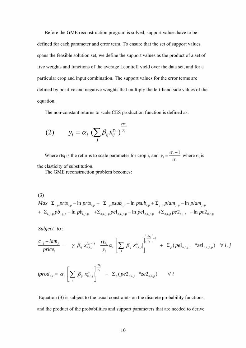
Before the GME reconstruction program is solved, support values have to be
defined for each parameter and error term. To ensure that the set of support values
spans the feasible solution set, we define the support values as the product of a set of
five weights and functions of the average Leontieff yield over the data set, and for a
particular crop and input combination. The support values for the error terms are
defined by positive and negative weights that multiply the left-hand side values of the
equation.
The non-constant returns to scale CES production function is defined as:
(2) ( )i
i i
rts
i i ij ijj
y xγ γα β= ∑
Where rtsi is the returns to scale parameter for crop i, and 1ii
i
σγσ−
= where σi is
the elasticity of substitution. The GME reconstruction problem becomes:
, , , , , , , , ,
, , , , , , , , , , , , , , , , , , , , ,
, ( 1), ,
(3)ln ln ln
ln 1 ln 1 2 ln 2
:
i
i p i p i p i p i p i p j p j p j p
i j p i j p i j p n i j p n i j p n i j p n i p n i p n i p
i j j ii ij n i j
i
Max prts prts psub psub plam plam
pb pb pe pe pe pe
Subject to
c lam rtsxprice
γγ β −
Σ − + Σ − + Σ −
+ Σ − +Σ − +Σ −
+=
1
, , , , , , , ,
, , , , , , ,
( 1 * 1 ) ,
( 2 * 2 )
i
ii
i
ii
rts
i ij n i j p n i j p n i j pji
rts
n i i ij n i j p n i p n i pj
x pe ze i j
tprod x pe ze i
γγ
γγ
α βγ
α β
⎛ ⎞−⎜ ⎟
⎝ ⎠⎡ ⎤+ Σ ∀⎢ ⎥
⎣ ⎦
⎡ ⎤= + Σ ∀⎢ ⎥
⎣ ⎦
∑
∑
`Equation (3) is subject to the usual constraints on the discrete probability functions,
and the product of the probabilities and support parameters that are needed to derive
10
the estimated coefficients for returns to scale ( rtsi ), elasticity of substitution ( σi ), the
shadow value of allocatable inputs ( lamj ), and the CES share parameters ( βij ). The
CES scale parameter is directly estimated without support values.
The objective function is the usual sum of the entropy measures for the parameter
probabilities. Following the normal GME procedure, the entropy of the error term
probabilities is also maximized. The first data based equations in ( 3 ) are the first
order conditions that set the cost ratio equal to the marginal physical product. If some
inputs are restricted, the input cost in the first order equation includes the estimated
shadow values as well as the nominal input price.
The second data based equations in ( 3 ) fit the production function to the
observations on total production. While it is not normal in econometric models to
include both the marginal and total products as estimating equations, we think that the
information in the total product constraint is particularly important for two reasons.
First, information on crop yields and areas is likely to be the most precisely know by
farmers. While farmers are often doubtful and reluctant about stating their costs of
production to surveyors, they always know their yields and are usually proud to tell
you. Second, while the marginal conditions are essential for behavioral analysis,
policy models also have to accurately fit the total product to be convincing to policy
makers and correctly estimate the total impact on the environment and the regional
economy of policy changes. Fitting the model to the integral as well as the marginal
conditions should improve the policy precision of the model.
Due to the separability assumption on the production functions, the estimation
problem can be solved rapidly by looping through individual production functions,
since the linkage between the production of different crops is defined by the shadow
values and allocatable input constraints.
11

We note that the supply functions, derived input demands, their associated
elasticities, and the elasticities of substitution are obtainable from a data set of any
size from one observation upwards. Clearly the reliance on the support space values
and the micro theory structural assumptions is much greater for minimal data sets.
However the approach does enable a formal approach to disaggregation of production
estimates, since the specification of the problem is identical for all sizes of data sets.
A problem for the widespread adoption of GME and entropy methods is the
frequent question from users of conventional estimates. “I accept that maximizing
entropy calculates an efficient distribution of the parameter, but how do I know that
the expected value of the parameter is a reliable point estimate”. In short, the potential
user is understandably asking for the variance of the coefficient. To date the response
from ME advocates is to reassure the potential user that the asymptotic properties are
consistent. This asymptotic response is not very reassuring for an estimator whose use
and comparative advantage is with small samples. It follows that there is a need to
generate GME parameter error bounds using the small data sets in which GME excels.
Using a Bootstrap (Efron & Tibsharani, 1993) method with the GME estimation
routine, we are able to generate variances for all the production function parameters
and corresponding pseudo t values. This will enable the analyst to have a formal
measure of precision for each parameter. In addition, having calculated the variance
of a set of critical policy parameters such as the disaggregated elasticities of
substitution and returns to scale, we can then apply statistical tests for significant
differences between the parameters and thus implicitly, the value of the farm size
disaggregation.
12
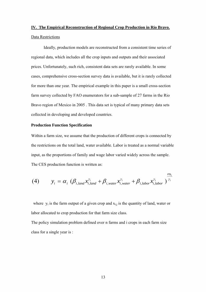
IV. The Empirical Reconstruction of Regional Crop Production in Rio Bravo.
Data Restrictions
Ideally, production models are reconstructed from a consistent time series of
regional data, which includes all the crop inputs and outputs and their associated
prices. Unfortunately, such rich, consistent data sets are rarely available. In some
cases, comprehensive cross-section survey data is available, but it is rarely collected
for more than one year. The empirical example in this paper is a small cross-section
farm survey collected by FAO enumerators for a sub-sample of 27 farms in the Rio
Bravo region of Mexico in 2005 . This data set is typical of many primary data sets
collected in developing and developed countries.
Production Function Specification
Within a farm size, we assume that the production of different crops is connected by
the restrictions on the total land, water available. Labor is treated as a normal variable
input, as the proportions of family and wage labor varied widely across the sample.
The CES production function is written as:
, , , , , ,(4) ( )i
i i i
rts
i i i land i land i water i water i labor i labory x x x iγ γ γ γα β β β= + +
where yi is the farm output of a given crop and xi,j is the quantity of land, water or
labor allocated to crop production for that farm size class.
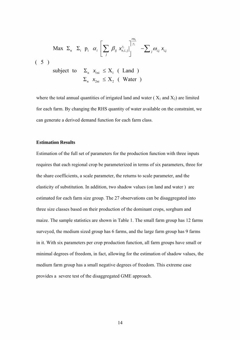
The policy simulation problem defined over n farms and i crops in each farm size
class for a single year is :
13
n i i , , i,j i,j
n 1ni 1
n 2ni 2
Max Σ Σ p
( 5 )subject to Σ X ( Land )
Σ X ( Water )
i
ii
rts
i ij n i j jj
x x
xx
γγα β ω
⎡ ⎤−⎢ ⎥
⎣ ⎦
≤≤
∑ ∑
where the total annual quantities of irrigated land and water ( X1 and X2) are limited
for each farm. By changing the RHS quantity of water available on the constraint, we
can generate a derived demand function for each farm class.
Estimation Results
Estimation of the full set of parameters for the production function with three inputs
requires that each regional crop be parameterized in terms of six parameters, three for
the share coefficients, a scale parameter, the returns to scale parameter, and the
elasticity of substitution. In addition, two shadow values (on land and water ) are
estimated for each farm size group. The 27 observations can be disaggregated into
three size classes based on their production of the dominant crops, sorghum and
maize. The sample statistics are shown in Table 1. The small farm group has 12 farms
surveyed, the medium sized group has 6 farms, and the large farm group has 9 farms
in it. With six parameters per crop production function, all farm groups have small or
minimal degrees of freedom, in fact, allowing for the estimation of shadow values, the
medium farm group has a small negative degrees of freedom. This extreme case
provides a severe test of the disaggregated GME approach.
14
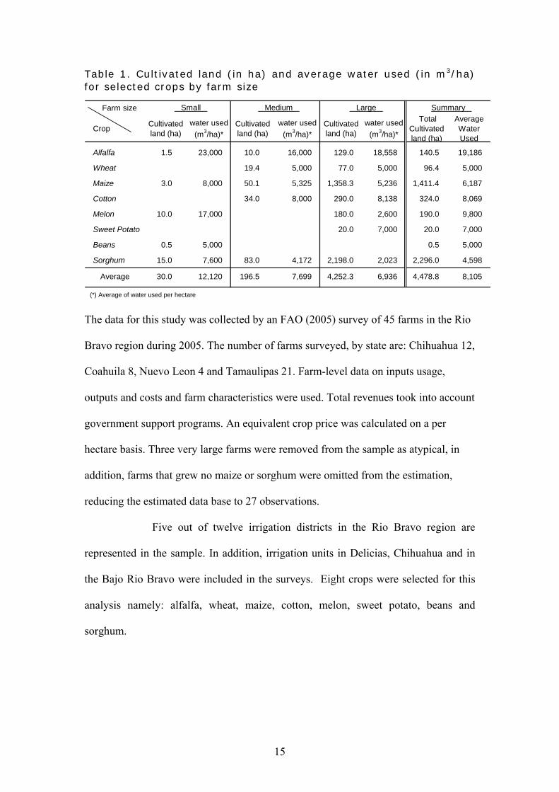
Table 1. Cultivated land (in ha) and average water used (in m3/ha) for selected crops by farm size
Farm size
Crop Cultivated land (ha)
water used (m3/ha)*
Cultivated land (ha)
water used (m3/ha)*
Cultivated land (ha)
water used (m3/ha)*
Total Cultivated land (ha)
Average Water Used
Alfalfa 1.5 23,000 10.0 16,000 129.0 18,558 140.5 19,186
Wheat 19.4 5,000 77.0 5,000 96.4 5,000
Maize 3.0 8,000 50.1 5,325 1,358.3 5,236 1,411.4 6,187
Cotton 34.0 8,000 290.0 8,138 324.0 8,069
Melon 10.0 17,000 180.0 2,600 190.0 9,800
Sweet Potato 20.0 7,000 20.0 7,000
Beans 0.5 5,000 0.5 5,000
Sorghum 15.0 7,600 83.0 4,172 2,198.0 2,023 2,296.0 4,598
Average 30.0 12,120 196.5 7,699 4,252.3 6,936 4,478.8 8,105
(*) Average of water used per hectare
Large Summary Small Medium
The data for this study was collected by an FAO (2005) survey of 45 farms in the Rio
Bravo region during 2005. The number of farms surveyed, by state are: Chihuahua 12,
Coahuila 8, Nuevo Leon 4 and Tamaulipas 21. Farm-level data on inputs usage,
outputs and costs and farm characteristics were used. Total revenues took into account
government support programs. An equivalent crop price was calculated on a per
hectare basis. Three very large farms were removed from the sample as atypical, in
addition, farms that grew no maize or sorghum were omitted from the estimation,
reducing the estimated data base to 27 observations.
Five out of twelve irrigation districts in the Rio Bravo region are
represented in the sample. In addition, irrigation units in Delicias, Chihuahua and in
the Bajo Rio Bravo were included in the surveys. Eight crops were selected for this
analysis namely: alfalfa, wheat, maize, cotton, melon, sweet potato, beans and
sorghum.
15
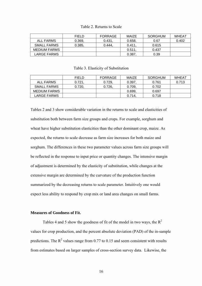
Table 2. Returns to Scale
FIELD FORRAGE MAIZE SORGHUM WHEAT ALL FARMS 0.369, 0.431, 0.658, 0.67 0.402
SMALL FARMS 0.385, 0.444, 0.411, 0.615 MEDIUM FARMS 0.511, 0.437 LARGE FARMS 0.387, 0.39
Table 3. Elasticity of Substitution
FIELD FORRAGE MAIZE SORGHUM WHEAT ALL FARMS 0.721, 0.729, 0.397, 0.761 0.713
SMALL FARMS 0.720, 0.726, 0.709, 0.702 MEDIUM FARMS 0.699, 0.697 LARGE FARMS 0.714, 0.718
Tables 2 and 3 show considerable variation in the returns to scale and elasticities of
substitution both between farm size groups and crops. For example, sorghum and
wheat have higher substitution elasticities than the other dominant crop, maize. As
expected, the returns to scale decrease as farm size increases for both maize and
sorghum. The differences in these two parameter values across farm size groups will
be reflected in the response to input price or quantity changes. The intensive margin
of adjustment is determined by the elasticity of substitution, while changes at the
extensive margin are determined by the curvature of the production function
summarized by the decreasing returns to scale parameter. Intuitively one would
expect less ability to respond by crop mix or land area changes on small farms.
Measures of Goodness of Fit.
Tables 4 and 5 show the goodness of fit of the model in two ways, the R2
values for crop production, and the percent absolute deviation (PAD) of the in-sample
predictions. The R2 values range from 0.77 to 0.15 and seem consistent with results
from estimates based on larger samples of cross-section survey data. Likewise, the
16
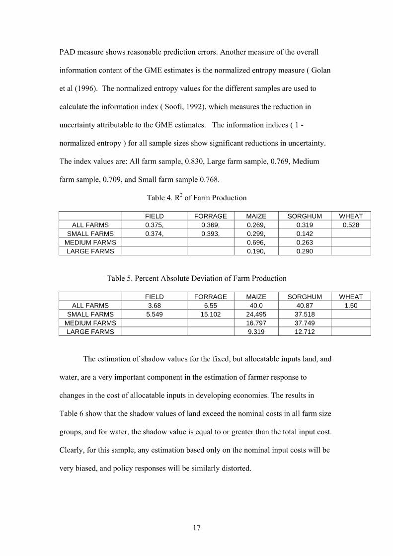
PAD measure shows reasonable prediction errors. Another measure of the overall
information content of the GME estimates is the normalized entropy measure ( Golan
et al (1996). The normalized entropy values for the different samples are used to
calculate the information index ( Soofi, 1992), which measures the reduction in
uncertainty attributable to the GME estimates. The information indices ( 1 -
normalized entropy ) for all sample sizes show significant reductions in uncertainty.
The index values are: All farm sample, 0.830, Large farm sample, 0.769, Medium
farm sample, 0.709, and Small farm sample 0.768.
Table 4. R2 of Farm Production
FIELD FORRAGE MAIZE SORGHUM WHEAT ALL FARMS 0.375, 0.369, 0.269, 0.319 0.528
SMALL FARMS 0.374, 0.393, 0.299, 0.142 MEDIUM FARMS 0.696, 0.263 LARGE FARMS 0.190, 0.290
Table 5. Percent Absolute Deviation of Farm Production
FIELD FORRAGE MAIZE SORGHUM WHEAT ALL FARMS 3.68 6.55 40.0 40.87 1.50
SMALL FARMS 5.549 15.102 24,495 37.518 MEDIUM FARMS 16.797 37.749 LARGE FARMS 9.319 12.712
The estimation of shadow values for the fixed, but allocatable inputs land, and
water, are a very important component in the estimation of farmer response to
changes in the cost of allocatable inputs in developing economies. The results in
Table 6 show that the shadow values of land exceed the nominal costs in all farm size
groups, and for water, the shadow value is equal to or greater than the total input cost.
Clearly, for this sample, any estimation based only on the nominal input costs will be
very biased, and policy responses will be similarly distorted.
17
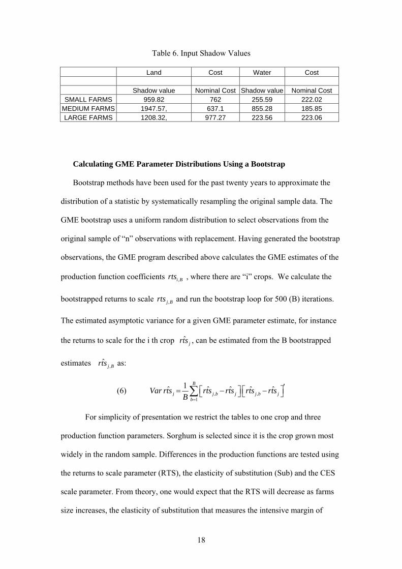
Table 6. Input Shadow Values
Land Cost Water Cost Shadow value Nominal Cost Shadow value Nominal Cost
SMALL FARMS 959.82 762 255.59 222.02 MEDIUM FARMS 1947.57, 637.1 855.28 185.85 LARGE FARMS 1208.32, 977.27 223.56 223.06
Calculating GME Parameter Distributions Using a Bootstrap
Bootstrap methods have been used for the past twenty years to approximate the
distribution of a statistic by systematically resampling the original sample data. The
GME bootstrap uses a uniform random distribution to select observations from the
original sample of “n” observations with replacement. Having generated the bootstrap
observations, the GME program described above calculates the GME estimates of the
production function coefficients , where there are “i” crops. We calculate the
bootstrapped returns to scale
,i Brts
,j Brts and run the bootstrap loop for 500 (B) iterations.
The estimated asymptotic variance for a given GME parameter estimate, for instance
the returns to scale for the i th crop , can be estimated from the B bootstrapped
estimates as:
ˆjrts
,ˆ
j Brts
, ,1
1ˆ ˆ ˆ ˆ(6)B
ˆj j b j j b j
bVar rts rts rts rts rts
B =
′⎡ ⎤ ⎡ ⎤= − −⎣ ⎦ ⎣ ⎦∑
For simplicity of presentation we restrict the tables to one crop and three
production function parameters. Sorghum is selected since it is the crop grown most
widely in the random sample. Differences in the production functions are tested using
the returns to scale parameter (RTS), the elasticity of substitution (Sub) and the CES
scale parameter. From theory, one would expect that the RTS will decrease as farms
size increases, the elasticity of substitution that measures the intensive margin of
18

adjustment has no theoretical reason to differ with farm size for the same crop, and
the scale parameter is expected to differ with farm size. Table 7 shows the mean and
variance of the three parameters by farm size
Table 7. Sorghum Production Parameters by Farm Size
Small Farm Medium Farm Large Farm
Mean Variance Mean Variance Mean Variance
RTS 0.615 0.02 ** 0.437 0.017 0.39 0.056 *
Substitution 0.615 0.263 0.688 0.019 ** 0.717 0.158 *
Scale 8.552 251.25 48.445 256863.53 125.5 28102.5
** significant at 1%, * significant at 5%. Question for Siwa—is it valid to calculate
the t values ?
The results in Table 7 show that, as expected, the returns to scale decrease
with larger farms, the elasticity of substitution shows no trend, and the scale
parameter increases. To formally evaluate whether there are significant differences in
these three parameters between the farm sizes, we used the bootstrap results to
generate pair-wise tests. The results are shown in Table 8 below.
Table 8. t values for differences in Sorghum Production Parameters
Small- Medium Small- Large Medium- Large
RTS 2.578 ** 2.721 ** 0.44
Substitution -0.338 -0.494 -0.170
Scale -0.276 -2.423 ** -0.423
19
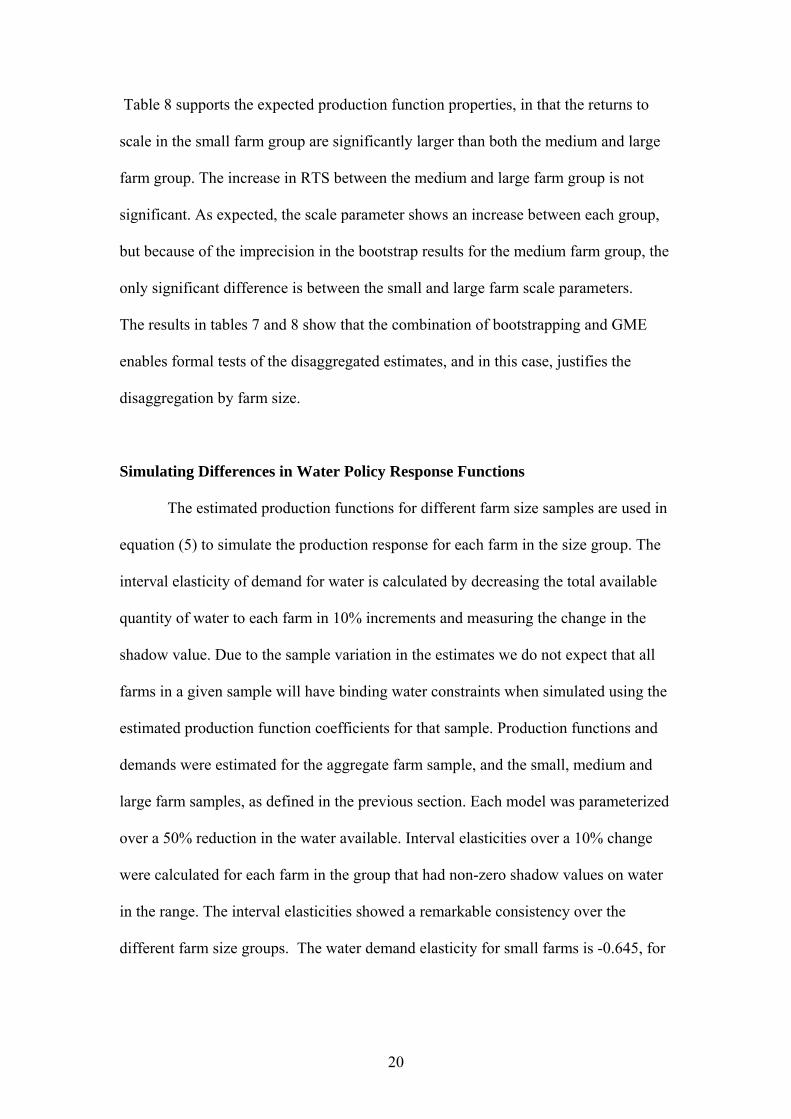
Table 8 supports the expected production function properties, in that the returns to
scale in the small farm group are significantly larger than both the medium and large
farm group. The increase in RTS between the medium and large farm group is not
significant. As expected, the scale parameter shows an increase between each group,
but because of the imprecision in the bootstrap results for the medium farm group, the
only significant difference is between the small and large farm scale parameters.
The results in tables 7 and 8 show that the combination of bootstrapping and GME
enables formal tests of the disaggregated estimates, and in this case, justifies the
disaggregation by farm size.
Simulating Differences in Water Policy Response Functions
The estimated production functions for different farm size samples are used in
equation (5) to simulate the production response for each farm in the size group. The
interval elasticity of demand for water is calculated by decreasing the total available
quantity of water to each farm in 10% increments and measuring the change in the
shadow value. Due to the sample variation in the estimates we do not expect that all
farms in a given sample will have binding water constraints when simulated using the
estimated production function coefficients for that sample. Production functions and
demands were estimated for the aggregate farm sample, and the small, medium and
large farm samples, as defined in the previous section. Each model was parameterized
over a 50% reduction in the water available. Interval elasticities over a 10% change
were calculated for each farm in the group that had non-zero shadow values on water
in the range. The interval elasticities showed a remarkable consistency over the
different farm size groups. The water demand elasticity for small farms is -0.645, for
20
medium farms -0.755, for large farms -0.691, and for the aggregated sample – 0.678.
These elasticity values are consistent with the majority of empirical analyses..
Despite this similarity in the interval elasticities, the derived demand functions
for different farm size groups differ greatly. To test the policy value of disaggregating
demand estimation by farm size, a demand function was obtained by regression on the
water quantities and shadow values generated for each farm in the sample when
parameterized by water reductions. Table 9 shows the fits and parameter values.
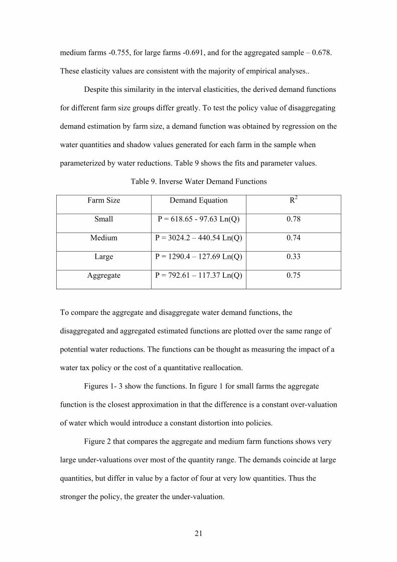
Table 9. Inverse Water Demand Functions
Farm Size Demand Equation R2
Small P = 618.65 - 97.63 Ln(Q) 0.78
Medium P = 3024.2 – 440.54 Ln(Q) 0.74
Large P = 1290.4 – 127.69 Ln(Q) 0.33
Aggregate P = 792.61 – 117.37 Ln(Q) 0.75
To compare the aggregate and disaggregate water demand functions, the
disaggregated and aggregated estimated functions are plotted over the same range of
potential water reductions. The functions can be thought as measuring the impact of a
water tax policy or the cost of a quantitative reallocation.
Figures 1- 3 show the functions. In figure 1 for small farms the aggregate
function is the closest approximation in that the difference is a constant over-valuation
of water which would introduce a constant distortion into policies.
Figure 2 that compares the aggregate and medium farm functions shows very
large under-valuations over most of the quantity range. The demands coincide at large
quantities, but differ in value by a factor of four at very low quantities. Thus the
stronger the policy, the greater the under-valuation.
21
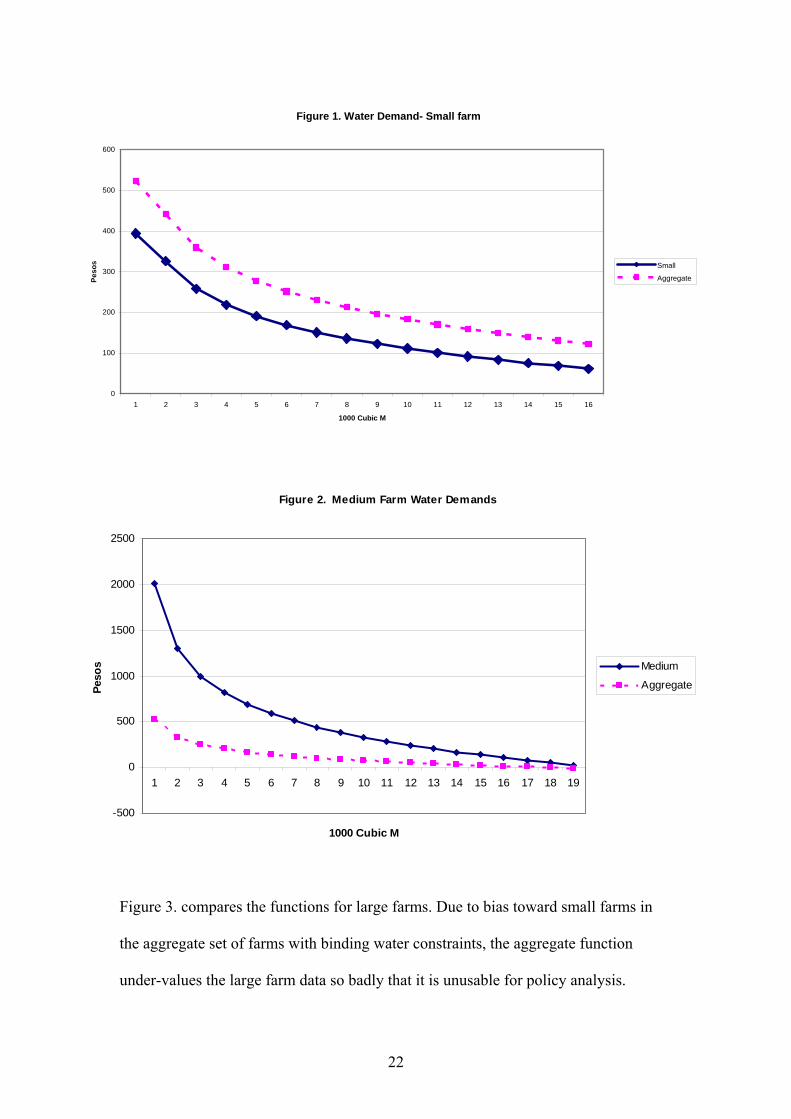
Figure 1. Water Demand- Small farm
0
100
200
300
400
500
600
1 2 3 4 5 6 7 8 9 10 11 12 13 14 15 16
1000 Cubic M
Peso
s Small
Aggregate
Figure 2. Medium Farm Water Demands
-500
0
500
1000
1500
2000
2500
1 2 3 4 5 6 7 8 9 10 11 12 13 14 15 16 17 18 19
1000 Cubic M
Peso
s Medium
Aggregate
Figure 3. compares the functions for large farms. Due to bias toward small farms in
the aggregate set of farms with binding water constraints, the aggregate function
under-values the large farm data so badly that it is unusable for policy analysis.
22
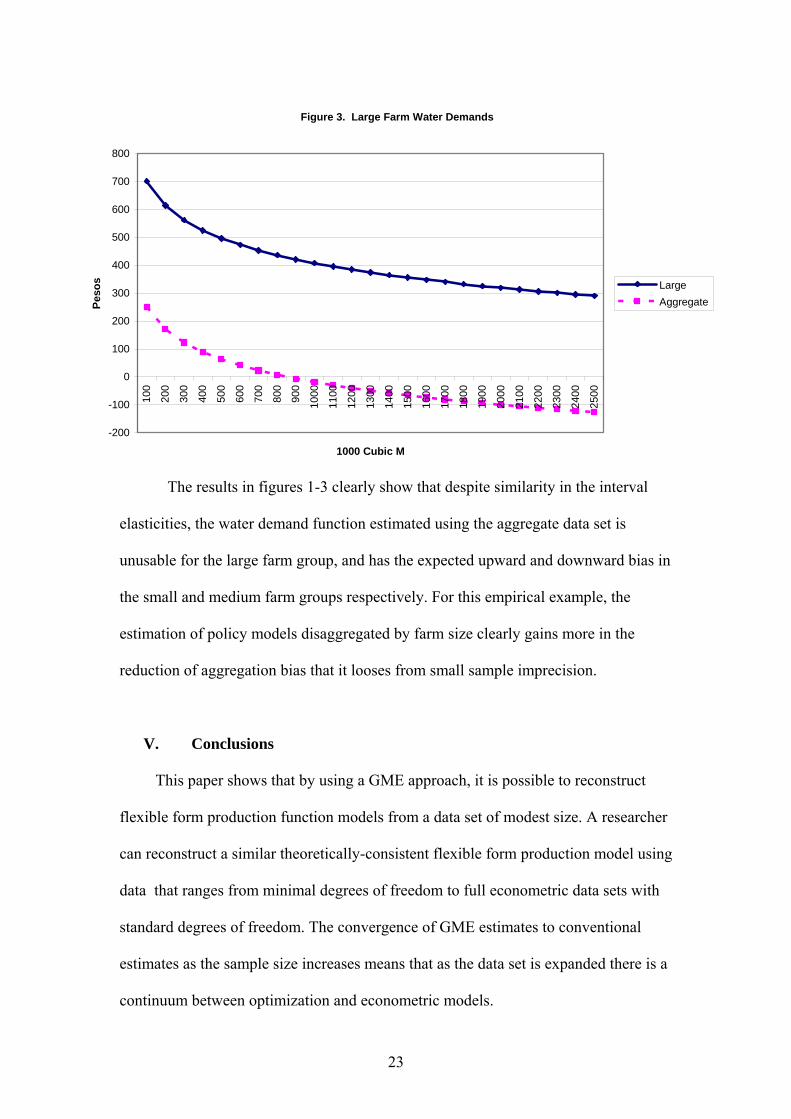
Figure 3. Large Farm Water Demands
-200
-100
0
100
200
300
400
500
600
700
80010
0
200
300
400
500
600
700
800
900
1000
1100
1200
1300
1400
1500
1600
1700
1800
1900
2000
2100
2200
2300
2400
2500
1000 Cubic M
Peso
s LargeAggregate
The results in figures 1-3 clearly show that despite similarity in the interval
elasticities, the water demand function estimated using the aggregate data set is
unusable for the large farm group, and has the expected upward and downward bias in
the small and medium farm groups respectively. For this empirical example, the
estimation of policy models disaggregated by farm size clearly gains more in the
reduction of aggregation bias that it looses from small sample imprecision.
V. Conclusions
This paper shows that by using a GME approach, it is possible to reconstruct
flexible form production function models from a data set of modest size. A researcher
can reconstruct a similar theoretically-consistent flexible form production model using
data that ranges from minimal degrees of freedom to full econometric data sets with
standard degrees of freedom. The convergence of GME estimates to conventional
estimates as the sample size increases means that as the data set is expanded there is a
continuum between optimization and econometric models.
23
The disaggregated production models yield all the comparative static properties
and parameters of large sample models. The effect of any constraints on inputs is
directly incorporated in the estimates through the simultaneous estimation of the
shadow values of the allocatable resources. An advantage of modeling production
functions is that they are readily understood by other disciplines, which are thus able
to add information for the prior support values or constraints.
In this example the aggregation bias in the aggregate model swamped any gains
in reducing the small sample error. The disaggregated model yielded greater precision
in its regional response. The gain from disaggregation of production models is an
empirical result that needs substantially more testing before one can conclude that it is
a common phenomenon. In this example, the empirical results show that the
disaggregated estimates have similar strong explanatory power as the aggregate
sample, as measured by R2, absolute deviation and the entropy information index.
Despite the similar measures of elasticity, the disaggregated samples show a wide
variation in the derived demand for water that directly influences policy response. The
use of disaggregated estimates is clearly supported by the results.
References
Alig, R.J., D.M. Adams and B.A. McCarl. " Impacts of Incorporating Land Exchanges Between Forestry and Agriculture in Sector Models." Journal of Agricultural and Applied Economics, 30:2 (1998): 389-401. Antle, J.M. & S. Capalbo. “Econometric-Process Models of Production.” American Journal of Agricultural Economics, 83 (May 2001): 389-401. Antle,J.M. & R.O. Valdivia. “ Modelling the supply of ecosystem services from agriculture: a minimum-data approach” Australian Journal of Agricultural & Resource Economics 50 (2006) : 1-15. Brooke, A., D. Kendrick, & A. Meeraus. "GAMS: A Users's Guide". The Scientific Press, 1988. Charnes, A., W.W. Cooper & E. Rhodes. “Measuring the Efficiency of Decision-Making Units.” European Journal of Operational Research, 2 (1985): 429-444.
24
Chambers, R. “Applied Production Analysis: The Dual Approach”, Cambridge University Press, Cambridge, 1988. Efron, B. and J. Tibsharani “ An Introduction to the Bootstrap” London, Chapman & Hall ( 1993 ). Golan, A., G. Judge, D. Miller. “Maximum Entropy Econometrics: Robust Estimation with Limited Data”, John Wiley & Sons, Chichester, England, 1996(a). Golan, A., G. Judge & J. Perloff. “Estimating the Size Distribution of Firms Using Government Summary Statistics.” J. Indust. Econ., 44 (Mar 1996(b)):69-80. Golan, A., G. Judge, S. Robinson. (1994) “Recovering Information from Incomplete or Partial Multisectoral Economic Data.” Rev. Econ. Statistics., 76 (Aug): 541-49. Heckelei, T. & W. Britz. "Concept and Explorative Application of an EU-wide, Regional Agricultural Sector Model (CAPRI-Project)". Presented at the 65th EAAE-Seminar, Bonn. March, 2000. Heckelei, T. and H. Wolff “ Estimation of constrained optimization models for agricultural supply analysis based on generalized maximum entropy” European Review of Agricultural Economics. (2003) vol 30, pp 27-50 Howitt, R. E. “Positive Mathematical Programming.” American Journal of Agricultural Economics, 77(Dec 1995):329-342. Howitt, R.E. & S. Msangi. “Consistency of GME Estimates Through Moment Constraints.” forthcoming Working Paper, Department of Agricultural and Resource Economics, University of California at Davis, 2002. Just,R.E., D Zilberman, and E. Hochman “Estimation of Multicrop Production Functions” American Journal of Agricultural Economics, 65 (1983): 770-780. Just, R.E., J.M. Antle.(1990) “Interactions Between Agricultural and Environmental Policies - A Conceptual Framework”. American Economic Review, 80:2(May):197-202. Lence, S. H. & D.J. Miller. “Estimation of Multi-Output Production Functions with Incomplete Data: A Generalized Maximum Entropy Approach.” Eur. Rev. Agr. Econ., 25(Dec 1988):188-209. Lence, S. H. & D.J. Miller. “Recovering Output-Specific Inputs from Aggregate Input Data: A Generalized Cross-Entropy Approach.” American Journal of Agricultural Economics, 80(Nov 1998):852-867. Love, H.A. “Conflicts Between Theory and Practice in Production Economics.” American Journal of Agricultural Economics, 81 (Aug 1999): 696–702.
25
Marsh, M.L. & R. Mittlehammer. “Adaptive Truncated Estimation Applied to Maximum Entropy.” Presented at the Western Agr. Econ. Assoc. Annual Meetings, Logan, Utah, (July 2001) 30 p. McCarl, B.A., D.M. Adams, R.J. Alig & J.T. Chmelik, "Analysis of Biomass Fuelled Electrical Power plants: Implications in the Agricultural and Forestry Sectors." Annals of Operations Research, 94(2000): 37-55. Mendelsohn, R., W.D. Nordhaus, D. Shaw. “The Impact of Global Warming on Agriculture: A Ricardian Analysis.” American Economic Review, 84 (Sep 1994): 753-771. Mittelhammer. R.C., G.G. Judge, D. J. Miller. “Econometric Foundations” New York : Cambridge University Press, 2000. Paris, Q. & R.E. Howitt. "Analysis of Ill-Posed Production Problems Using Maximum Entropy." American Journal of Agricultural Economics, 80 (Aug 1988):124-138. Paris, Q. “Multicollinearity and Maximum Entropy Estimators.” Economics Bulletins, 3 (no. 11, 2001):1-9. Paris, Q. & M. Caputo. “Sensitivity of the GME Estimates to Support Bounds.” Working Paper, Department of Agricultural and Resource Economics, University of California at Davis, (Aug 2001) 18 p. Soofi, E.S. “Capturing the intangible concept of information” Journal of the American Statistical Association, 89 (1994): 1243-54.. US Department of the Interior, Bureau of Reclamation.(1997) “ Central Valley Project Improvement Act: Draft Programmatic Environmental Impact Statement”, Sacramento, California.. (S. Hatchett main author of CVPM model description in Technical Appendix) Wu, J.J. & B. Babcock. “Meta-modeling Potential Nitrate Water Pollution in the Central United States.” Journal of Environmental Quality, 28( Nov-Dec, 1999):1916-28. Zhang, X. & S. Fan. “Crop-Specific Production Technologies in Chinese Agriculture.” American Journal of Agricultural Economics, 83 (May 2001): 378-388.
26